Sparse Recovery and Dictionary Learning from Nonlinear Compressive Measurements

Abstract

Sparse coding and dictionary learning are popular techniques for linear inverse problems such as denoising or inpainting. However in many cases, the measurement process is nonlinear, for example for clipped, quantized or 1-bit measurements. These problems have often been addressed by solving constrained sparse coding problems, which can be difficult to solve, and assuming that the sparsifying dictionary is known and fixed. Here we propose a simple and unified framework to deal with nonlinear measurements. We propose a cost function that minimizes the distance to a convex feasibility set, which models our knowledge about the nonlinear measurement. This provides an unconstrained, convex, and differentiable cost function that is simple to optimize, and generalizes the linear least squares cost commonly used in sparse coding. We then propose proximal based sparse coding and dictionary learning algorithms, that are able to learn directly from nonlinearly corrupted signals. We show how the proposed framework and algorithms can be applied to clipped, quantized and 1-bit data.

I Introduction

Sparse decomposition and dictionary learning are popular techniques for linear inverse problems in signal processing, such as denoising [1, 2], inpainting [3, 4] or super-resolution [5, 6]. Sparse coding aims at finding a sparse set of coefficients $\operatorname{\bm{\alpha}}\in\mathbb{R}^{M}$ that accurately represents a signal ${\mathbf{x}}\in\mathbb{R}^{N}$ from a fixed overcomplete dictionary ${\mathbf{D}}\in\mathbb{R}^{N\times M}$, and is often formulated as:

$$\min_{\bm{\alpha}}\|{\mathbf{x}}-{\mathbf{D}}\operatorname{\bm{\alpha}}\|_{2}^{2}\quad+\lambda\Psi(\operatorname{\bm{\alpha}}),$$ (1)

where $\Psi(\cdot)$ is a sparsity inducing regularizer, such as the $\ell_{0}$ pseudo-norm or the $\ell_{1}$-norm. Dictionary learning on the other hand, jointly learns the dictionary ${\mathbf{D}}$ and sparse coefficients $\operatorname{\bm{\alpha}}_{t}$ from a set of training signals $\{{\mathbf{x}}_{t}\}_{t=1,\dotsc,T}$:

$$\min_{{\mathbf{D}},\bm{\alpha}_{t}}\sum_{t=1}^{T}\left[\|{\mathbf{x}}_{t}-{\mathbf{D}}\operatorname{\bm{\alpha}}_{t}\|_{2}^{2}\quad+\lambda\Psi(\operatorname{\bm{\alpha}}_{t})\right].$$ (2)

However, the observed signals are often distorted or measured in a nonlinear way:

$$\mathbf{y}=f({\mathbf{x}}),$$ (3)

where $f$ is a nonlinear measurement function, and ${\mathbf{x}}$ is the original (unknown) clean signal. Examples of nonlinear distortions include clipping (or saturation) and quantization. Clipping is often due to dynamic range limitations in acquisition systems, when a signal reaches a maximum allowed amplitude, and the waveform is truncated above that threshold [7, 8, 9, 10, 11, 12, 13, 14]. Quantization is a common process in analog-to-digital conversion that maps a signal from a continuous input space to a (finite) discrete space [15]. More recently, 1-bit compression has attracted a lot of interest, as an extreme quantization scheme where samples are coded using only one bit per sample [16], i.e. only measuring the signs of the signal. Clipping and quantization are non-linear, non-smooth, and compressive measurements, i.e. the measurement map is non-invertible. For these reasons, the recovery of clipped/quantized signals is a challenging problem.

Recovering a signal from clipped or quantized measurements can be treated as linear inverse problems, by simply ignoring the nonlinearities, i.e. treating clipped samples as missing [17, 8] and quantization error as additive noise [18]. Similarly, 1-bit signals can be tackled by using the sign measurements directly as an input [16, 19]. However using a formulation that is consistent with the measurement process, i.e. that takes into account our knowledge about the nonlinear measurement function, has been shown to greatly improve the reconstruction [7, 8, 9, 4, 10, 11, 12, 13, 14, 20, 21, 22, 23, 24, 16, 19, 25]. Specially tailored cost functions, constraints, or regularizers have independently been proposed to deal with clipped [7, 8, 9, 4, 10, 11, 12, 13, 14], quantized [20, 21, 22, 23, 24] or 1-bit [16, 19, 25] measurements. These formulations often involve solving constrained sparse coding problems, which can be difficult and computationally expensive to solve, since they involve computing expensive non-orthogonal projections at each iteration [13, 24].

Reconstruction methods proposed in the literature assume that the signal is sparse in some orthogonal basis [21, 20, 22, 23, 24, 26, 16, 19, 25, 23], or in a fixed dictionary [9, 4, 10, 13]. However it has been shown in a range of applications (when the measurements are linear), that learning the dictionary from the observed data greatly improves the reconstruction compared to using a fixed dictionary [1, 2, 27, 28].

I-A Contributions, and main results

Our contributions are as follows:

• We propose a unifying framework for signal recovery from nonlinear measurements such as clipping, quantization and 1-bit measurements, i.e. addressing these three problems in a unified fashion rather than individually. More specifically, we show how these problems can be formulated as minimizing the distance to a convex feasibility set, which models our assumption about the nonlinear measurement process. In particular, the proposed cost generalizes the linear least squares commonly used in sparse coding, as well as several cost functions proposed independently for declipping and 1-bit recovery.

• Using properties of projection operators over convex sets, we show that the proposed cost function is continuous, convex and differentiable with Lipschitz gradient. Our main result uses Danskin’s Min-Max theorem [29], that allows us to derive a closed-form gradient for the proposed cost.

• We propose proximal-based consistent sparse coding, and dictionary learning algorithms, for nonlinear measurements. We show that these algorithms can be applied to clipped, quantized and 1-bit measurements.

I-B Organization of paper

The paper is organised as follows: in Section II, we briefly review sparse recovery and dictionary learning from linear measurements, and some strategies proposed to deal with clipped, quantized and 1-bit measurements. In Section III we propose a unifying cost function for nonlinear measurements, and show some of its properties. In Section IV we propose consistent sparse coding and dictionary learning algorithms using the proposed cost. Applications of the proposed framework, and links to previous work are presented in Section V. The performance of the proposed algorithm is presented in Section VI, before the conclusion is drawn.

I-C Notation

Bold lowercase letters ${\mathbf{x}}$ denote vectors and bold uppercase letters ${\mathbf{X}}$ denote matrices. The $i$-th element of a vector ${\mathbf{x}}$ is noted $x_{i}$. The identity matrix is noted ${\mathbf{I}}$. The p-norm of a vector ${\mathbf{x}}$ is $\|{\mathbf{x}}\|_{p}=(\sum x_{i}^{p})^{1/p}$. The $\ell_{0}$ pseudo-norm (i.e. the number of non-zero elements) of ${\mathbf{x}}$ is noted $\|{\mathbf{x}}\|_{0}$. For a matrix ${\mathbf{X}}$, $\|{\mathbf{X}}\|_{2}$ denotes the matrix 2-norm, i.e. the largest singular value of ${\mathbf{X}}$. We denote $({\mathbf{x}})_{+}=\max(\mathbf{0},{\mathbf{x}})$ (where $\max$ is the element-wise maximum), and $({\mathbf{x}})_{-}=-(-{\mathbf{x}})_{+}$. The floor (i.e. closest lower integer) of a vector is noted $\lfloor{\mathbf{x}}\rfloor$ (applied element-wise). The sign (positive or negative) of each element of ${\mathbf{x}}$ is noted $\operatorname*{sign}({\mathbf{x}})$. The element-wise multiplication is $\odot$. For a set $\mathcal{C}$, $\operatorname*{cl}(\mathcal{C})$ is the closure of $\mathcal{C}$, and $\mathbbm{1}_{\mathcal{C}}(\cdot)$ is the indicator function of that set, i.e. $\mathbbm{1}_{\mathcal{C}}({\mathbf{x}})=0$ when ${\mathbf{x}}\in\mathcal{C}$, $+\infty$ otherwise. The notation $\preceq$ denotes vector-wise inequality.

II Background

In this paper, we denote observation vectors as $\mathbf{y}\in\mathbb{R}^{L}$, with $\mathbf{y}=f({\mathbf{x}})$, where ${\mathbf{x}}\in\mathbb{R}^{N}$ is the original un-observed clean signal, and $f$ is a measurement or distortion function. We further assume that the signal ${\mathbf{x}}$ can be decomposed as ${\mathbf{x}}={\mathbf{D}}\operatorname{\bm{\alpha}}$ with ${\mathbf{D}}\in\mathbb{R}^{N\times M}$ an overcomplete dictionary of $M$ atoms ($N<M$), and $\operatorname{\bm{\alpha}}\in\mathbb{R}^{M}$ is a sparse activation vector. In this section we review the different types of linear and nonlinear measurement functions $f$, and the associated problem formulations appearing in the literature.

II-A Sparse coding from linear measurements

A widely studied case is when the measurement function is linear, i.e. $f({\mathbf{x}})={\mathbf{M}}{\mathbf{x}}$ with ${\mathbf{M}}\in\mathbb{R}^{L\times N}$. The corresponding sparse coding problem is often formulated as:

$$\min_{\operatorname{\bm{\alpha}}}\|\mathbf{y}-{\mathbf{M}}{\mathbf{D}}\operatorname{\bm{\alpha}}\|_{2}^{2}+\lambda\Psi(\operatorname{\bm{\alpha}}).$$ (4)

For example, ${\mathbf{M}}={\mathbf{I}}$ (the identity matrix) corresponds to clean signals or signals subject to additive Gaussian noise [1, 2]. When ${\mathbf{M}}$ is a diagonal binary matrix, (4) corresponds to an inpainting problem [3, 4].

II-B Sparse coding from nonlinear measurements

Sparse coding from linear measurements have been extensively studied in the literature. Signal acquisition systems however often measure signals in a nonlinear way, for examples in saturated, quantized or 1-bit measurements. In the following, we review reconstruction strategies proposed in the literature for saturated, quantized and 1-bit measurements.

(a) Clipping

(b) Quantization

(c) 1-bit sensing

Figure 1: Visualization of different nonlinear measurement functions $f$ (output $y_{i}=f(x_{i})$ versus input $x_{i}$).

II-B1 Clipped measurements

We consider the case of hard clipping, where each sample $x_{i}$ is measured as:

$$y_{i}=f(x_{i})=\begin{cases}\theta^{+}\quad\text{if}\quad x_{i}\geq\theta^{+}\\ \theta^{-}\quad\text{if}\quad x_{i}\leq\theta^{-}\\ x_{i}\quad\text{otherwise,}\end{cases}$$ (5)

where $\theta^{+}>\theta^{-}$ are positive and negative clipping thresholds respectively (Figure 1(a)). This can be written in vector form as:

$$\mathbf{y}=f({\mathbf{x}})=\operatorname{\mathbf{M^{r}}}{\mathbf{x}}+\theta^{+}\operatorname{\mathbf{M^{c+}}}\mathbf{1}+\theta^{-}\operatorname{\mathbf{M^{c-}}}\mathbf{1},$$ (6)

where $\mathbf{1}$ is the all-ones vector in $\mathbb{R}^{N}$, and $\operatorname{\mathbf{M^{r}}},\operatorname{\mathbf{M^{c+}}}$ and $\operatorname{\mathbf{M^{c-}}}$ are diagonal binary sensing matrices, that define the reliable (i.e. unclipped), positive and negative clipped samples respectively and such that $\operatorname{\mathbf{M^{r}}}+\operatorname{\mathbf{M^{c+}}}+\operatorname{\mathbf{M^{c-}}}={\mathbf{I}}$. In practice, the clipping thresholds can be estimated from the measurement $\mathbf{y}$ as (e.g.) $\theta^{+}=\max_{i}(y_{i})$, and the sensing matrices as $[\operatorname{\mathbf{M^{c+}}}]_{i,i}=1$ if $y_{i}=\theta^{+}$, $0$ otherwise.

Declipping can be treated as a linear inverse problem by discarding the clipped samples, treating declipping as a linear inpainting problem, i.e. solving (4) with ${\mathbf{M}}=\operatorname{\mathbf{M^{r}}}$ [17, 8, 4]. However, the reconstruction can be improved by adding extra knowledge about the clipping process. Indeed, we know that the clipped samples should have an amplitude that is greater than the clipping threshold. This extra information can be enforced by solving the following constrained problem [30, 7, 9, 11, 14]:

$$\min_{\operatorname{\bm{\alpha}}}\Psi(\operatorname{\bm{\alpha}})+\mathbbm{1}_{\mathcal{C}(\mathbf{y})}({\mathbf{D}}\operatorname{\bm{\alpha}}),$$ (7)

where:

$$\begin{split}\mathcal{C}(\mathbf{y})\triangleq\{{\mathbf{x}}|\operatorname{\mathbf{M^{r}}}&\mathbf{y}=\operatorname{\mathbf{M^{r}}}{\mathbf{x}},\operatorname{\mathbf{M^{c+}}}{\mathbf{x}}\succeq\theta^{+}\operatorname{\mathbf{M^{c+}}}\mathbf{1},\\ &\operatorname{\mathbf{M^{c-}}}{\mathbf{x}}\preceq\theta^{-}\operatorname{\mathbf{M^{c-}}}\mathbf{1}\}\end{split}$$ (8)

is the clipping consistency set. Eqn. (7) is a constrained, non-smooth and possibly non-convex sparse decomposition problem, which can be difficult to solve. An alternating direction method of multipliers (ADMM) [31] based algorithm was proposed in [13] to solve (7). When the dictionary is a tight frame, the algorithm can be computed efficiently [32]. However, for general dictionaries, the algorithm is computationally expensive, since it involves computing non-orthogonal projections at each iteration [13]. A soft consistency metric was used in [8, 10, 12]:

$$\begin{split}\min_{\operatorname{\bm{\alpha}}}\frac{1}{2}\big{[}\|\operatorname{\mathbf{M^{r}}}&(\mathbf{y}-{\mathbf{D}}\operatorname{\bm{\alpha}})\|_{2}^{2}+\|\operatorname{\mathbf{M^{c+}}}(\theta^{+}\mathbf{1}-{\mathbf{D}}\operatorname{\bm{\alpha}})_{+}\|_{2}^{2}\\ +&\|\operatorname{\mathbf{M^{c-}}}(\theta^{-}\mathbf{1}-{\mathbf{D}}\operatorname{\bm{\alpha}})_{-}\|_{2}^{2}\big{]}+\lambda\Psi(\operatorname{\bm{\alpha}}),\end{split}$$ (9)

The data-fidelity term in (9) is convex and smooth, so methods based on iterative hard thresholding [33, 10] or proximal algorithms [34, 12] can directly be applied.

II-B2 Quantized measurements

Quantization maps a continuous input space onto a finite discrete set of codewords $\mathcal{Y}=\{y_{1},...,y_{p}\}$. A quantization map $f$ is defined by a set of quantization levels $\mathcal{R}_{q}=[l_{q},u_{q})$ and the relation $x\in\mathcal{R}_{q}\Leftrightarrow f(x)=y_{q}$, i.e. samples that fall into $\mathcal{R}_{q}$ are quantized as $y_{q}$. For example in the case of a uniform mid-riser quantizer, $\mathcal{R}_{q}=[\Delta q,\Delta(q+1))$, and the quantization function can be written as:

$$f({\mathbf{x}})=\Delta\left\lfloor\frac{{\mathbf{x}}}{\Delta}\right\rfloor+\frac{\Delta}{2},$$ (10)

where $\Delta>0$ is the quantization bin width (Figure 1(b)).

De-quantization can be treated as a simple linear inverse problem by considering quantization error as additive noise, and using a linear sparse model (4) [18]. However it has been shown that using a more accurate model of the quantization process improves the reconstruction. Bayesian approaches [21], $\ell_{p}$-based data-fidelity terms [22], or specially-tailored cost functions [23] have been proposed in the literature to enforce quantization consistency. Constrained formulations were proposed in [20, 24] in order to enforce consistency:

$$\min_{\operatorname{\bm{\alpha}}}\Psi(\operatorname{\bm{\alpha}})+\mathbbm{1}_{\mathcal{R}}({\mathbf{D}}\operatorname{\bm{\alpha}})$$ (11)

where $\mathcal{R}=\mathcal{R}_{q_{1}}\times...\times\mathcal{R}_{q_{N}}$ and $\mathcal{R}_{q_{i}}$ is the quantization region associated with the $i$-th sample $y_{i}$. However similarly to the constrained declipping scenario (7), solving (11) can be computationally expensive.

II-B3 1-bit measurements

1-bit measurement can be seen as an extreme quantization using only one bit per sample, or similarly an extreme saturation where the clipping level tends to zero:

$$f({\mathbf{x}})=\operatorname*{sign}({\mathbf{x}}).$$ (12)

1-bit measurement consistency has also been proposed in [16, 19]:

$$\min_{\operatorname{\bm{\alpha}}}\frac{1}{2}\|\big{(}\mathbf{y}\odot({\mathbf{D}}\operatorname{\bm{\alpha}})\big{)}_{-}\|_{2}^{2}+\lambda\Psi(\operatorname{\bm{\alpha}})$$ (13)

II-C Dictionary learning

Dictionary learning from linear measurements can be formulated as [28]:

$$\min_{{\mathbf{D}}\in\mathcal{D},\bm{\alpha}_{t}}\sum_{t=1}^{T}\big{[}\|{\mathbf{x}}_{t}-{\mathbf{D}}\operatorname{\bm{\alpha}}_{t}\|_{2}^{2}+\lambda\Psi(\operatorname{\bm{\alpha}}_{t})\big{]}$$ (14)

where $\{{\mathbf{x}}_{t}\}_{1...T}$ is a collection of $T$ signals in $\mathbb{R}^{N}$, and $\operatorname{\bm{\alpha}}_{t}$ are the corresponding sparse activation vectors. The dictionary ${\mathbf{D}}$ is often constrained to be in the convex set $\mathcal{D}=\{{\mathbf{D}}\in\mathbb{R}^{N\times M}|\forall i,\|\mathbf{d}_{i}\|_{2}\leq 1\}$ in order to avoid scaling ambiguity [28]. Many algorithms have been proposed in the literature to solve (14), such as MOD [35], K-SVD [1] stochastic gradient descent [36, 37], or SimCO [38].

Dictionary learning for 1-bit data have recently been addressed in [39, 40]. To our knowledge, dictionary learning from saturated and quantized measurements, however, has not been addressed in the literature. In the next sections, we propose a unifying and computationally tractable framework for sparse coding and dictionary learning from nonlinear measurements.

III A unifying framework for nonlinear signal reconstruction

Let $f:\mathcal{X}\mapsto f(\mathcal{X})=\mathcal{Y}$ be an arbitrary - and possibly nonlinear - measurement function from a clean input space $\mathcal{X}$ to a measurement space $\mathcal{Y}$. For a measured signal $\mathbf{y}\in\mathcal{Y}$, we propose a cost function (or data-fidelity term) defined for all ${\mathbf{x}}\in\mathcal{X}$ as:

$$\mathcal{L}_{f}({\mathbf{x}},\mathbf{y})=\operatorname*{d}({\mathbf{x}},f^{-1}\{\mathbf{y}\})$$ (15)

where $f^{-1}\{\mathbf{y}\}$ is the pre-image of $\{\mathbf{y}\}$ under the measurement map $f$:

$$f^{-1}\{\mathbf{y}\}\triangleq\{{\mathbf{x}}\in\mathcal{X}|f({\mathbf{x}})=\mathbf{y}\},$$ (16)

and $\operatorname*{d}({\mathbf{x}},\mathcal{C})$ is the distance between ${\mathbf{x}}$ and the set $\mathcal{C}$, defined for a (pointwise) distance metric $\operatorname*{d}(\cdot,\cdot)$ as:

$$\operatorname*{d}({\mathbf{x}},\mathcal{C})\triangleq\inf_{{\mathbf{z}}\in\mathcal{C}}\operatorname*{d}({\mathbf{x}},{\mathbf{z}}).$$ (17)

The set $f^{-1}\{\mathbf{y}\}$ can be seen as a feasibility set, i.e. the set of all possible input signals ${\mathbf{x}}\in\mathcal{X}$ that could have generated $\mathbf{y}$ when measured through $f$. The cost (15) thus measures how “close” a signal ${\mathbf{x}}$ is to the feasibility set associated with the measurement $\mathbf{y}$. Minimizing (15) thus promotes consistency since it minimizes the distance between an estimate ${\mathbf{x}}$ and its feasibility set $f^{-1}\{\mathbf{y}\}$. However unlike constrained formulations (7) or (11), here measurement-consistency is enforced in a simple unconstrained way.

III-A Assumptions on $f$, and choice of distance

Without any assumptions on the feasibility sets $f^{-1}\{\mathbf{y}\}$ and the metric $\mathbf{d}(\cdot,\cdot)$, ${\mathbf{x}}\mapsto\mathcal{L}_{f}({\mathbf{x}},\mathbf{y})$ is in general non-convex and non-smooth, and therefore difficult to optimize. However we show here that under certain conditions, the proposed cost (15) exhibits convenient properties such as convexity, and differentiability with Lipschitz gradient.

The first assumption is that for all $\mathbf{y}\in\mathcal{Y}$, the pre-image set $f^{-1}\{\mathbf{y}\}$ is convex. This assumption is verified by many measurement functions $f$ found in practice, such as linear measurements, and nonlinear measurements such as clipping, quantization and 1-bit (see Section V). For separable functions $f({\mathbf{x}})=\left[f_{1}(x_{1}),\dotsc,f_{N}(x_{N})\right]$, a simple sufficient condition such that $f^{-1}\{\mathbf{y}\}$ is convex for all $\mathbf{y}$ is that each $f_{i}(\cdot)$ is monotonic (but not necessarily strictly monotonic). This condition is however not necessary, and the set of functions with convex pre-images includes a wider range of measurement functions. Convexity of the pre-image sets ensures that the proposed cost (15) is convex and differentiable, as will be shown in this section.

Various metrics can be chosen for the pointwise distance in (17). A popular metric to measure point-wise distances is the squared Euclidean distance $\|\cdot\|_{2}^{2}$. The squared Euclidean distance, or least squares, is popular in sparse coding and dictionary learning, in part due to its convexity and Lipschitz differentiability. Other pointwise distances are available, such as $p$-norms $\|\cdot\|_{p}^{p}$ with $0<p\leq 1$, which might be more appropriate depending on the data at hand. However these come at a cost of non-differentiability and/or non-convexity, which often lead to more difficult optimization problems. In this paper, for simplicity, and in order to favour computationally efficient methods, we focus on the least-squares distance. In fact, we show in this section that the proposed cost (15) benefits from the same properties as – and naturally extends – the linear least-squares cost commonly used in sparse coding.

In the remainder of this paper, we assume $\mathcal{X}=\mathbb{R}^{N}$, $\mathbf{d}({\mathbf{x}},\mathbf{y})=\frac{1}{2}\|{\mathbf{x}}-\mathbf{y}\|_{2}^{2}$, and $f^{-1}\{\mathbf{y}\}$ convex for all $\mathbf{y}\in\mathcal{Y}$. Note that for a set $\mathcal{C}$, $\operatorname*{d}({\mathbf{x}},\mathcal{C})=\operatorname*{d}({\mathbf{x}},\operatorname*{cl}(\mathcal{C}))$, so we can assume without loss of generality that $f^{-1}\{\mathbf{y}\}$ is closed. Note also that since $\mathcal{Y}=f(\mathcal{X})$, $f^{-1}\{\mathbf{y}\}$ is non-empty for all $\mathbf{y}\in\mathcal{Y}$.

III-B Properties of the proposed cost function

We consider a fixed $\mathbf{y}\in\mathcal{Y}$, and review the properties of ${\mathbf{x}}\mapsto\mathcal{L}_{f}({\mathbf{x}},\mathbf{y})$. Since $f^{-1}\{\mathbf{y}\}$ is non-empty, closed and convex, the Projection Theorem (Appendix A) ensures existence and uniqueness of a minimizer ${\mathbf{z}}^{*}$ of $\|{\mathbf{x}}-{\mathbf{z}}\|^{2}_{2}$ in $f^{-1}\{\mathbf{y}\}$. This minimizer is defined as the orthogonal projection $\Pi_{f^{-1}\{\mathbf{y}\}}({\mathbf{x}})$ of ${\mathbf{x}}$ on the set $f^{-1}\{\mathbf{y}\}$. In particular, the infinimum in (17) is attained, and $\mathcal{L}_{f}({\mathbf{x}},\mathbf{y})$ can be redefined as:

$$\mathcal{L}_{f}({\mathbf{x}},\mathbf{y})=\frac{1}{2}\|{\mathbf{x}}-\Pi_{f^{-1}\{\mathbf{y}\}}({\mathbf{x}})\|_{2}^{2}.$$ (18)

In addition, the continuity property of the projection operator on a convex set ensures that $\mathcal{L}_{f}(\cdot,\mathbf{y})$ is a continuous function (as a composition of continuous functions). We now present some properties of $\mathcal{L}_{f}(\cdot,\mathbf{y})$, which make it suitable for a range of optimization algorithms:

Proposition 1.

$\mathcal{L}_{f}(\cdot,\mathbf{y})$ is a convex cost function.

Proposition 2.

$\mathcal{L}_{f}(\cdot,\mathbf{y})$ is differentiable, with gradient:

$$\nabla_{\mathbf{x}}\mathcal{L}_{f}({\mathbf{x}},\mathbf{y})={\mathbf{x}}-\Pi_{f^{-1}\{\mathbf{y}\}}({\mathbf{x}}).$$ (19)

Proposition 3.

The gradient $\nabla_{{\mathbf{x}}}\mathcal{L}_{f}({\mathbf{x}},\mathbf{y})$ is Lipschitz continuous with constant $L=1$, i.e. for all ${\mathbf{x}}_{1},{\mathbf{x}}_{2}$:

$$\|\nabla_{{\mathbf{x}}}\mathcal{L}_{f}({\mathbf{x}}_{1},\mathbf{y})-\nabla_{{\mathbf{x}}}\mathcal{L}_{f}({\mathbf{x}}_{2},\mathbf{y})\|^{2}_{2}\leq\|{\mathbf{x}}_{1}-{\mathbf{x}}_{2}\|_{2}^{2}$$ (20)

Proposition 1 is due to the convexity of the set $f^{-1}\{\mathbf{y}\}$ and of the least-squares cost. Proposition 2 is a direct consequence of Danskin’s Min-Max theorem (Appendix B) and of the uniqueness of the projection operator. Proposition 3 is a consequence of the contraction property of projection onto convex sets. See Appendix C for more detailed proofs.

Continuity, convexity and Lipschitz differentiability makes the proposed cost function suitable for a range of optimization algorithm as will be seen in the next section. Moreover, when $f$ is the identity map ($f({\mathbf{x}})={\mathbf{x}}$), we have $f^{-1}\{\mathbf{y}\}=\mathbf{y}$ and $\mathcal{L}_{f}({\mathbf{x}},\mathbf{y})=\frac{1}{2}\|{\mathbf{x}}-\mathbf{y}\|_{2}^{2}$. The proposed cost thus generalizes the least squares cost commonly used in sparse coding and dictionary learning. We will show in Section V how the proposed cost also generalizes several cost functions proposed in the literature for inpainting, declipping and 1-bit signals, and how it can be applied to quantized measurements. The proposed cost thus provides a unifying framework to tackle all these problems. In the next section we propose simple proximal-based algorithms for sparse coding and dictionary learning using the proposed cost.

IV Proposed consistent sparse coding and dictionary learning algorithms

IV-A Sparse coding algorithms

For a nonlinear observation $\mathbf{y}$ and a fixed dictionary ${\mathbf{D}}$, we propose to formulate consistent sparse coding as:

$$\min_{\bm{\alpha}}\mathcal{L}_{f}({\mathbf{D}}\operatorname{\bm{\alpha}},\mathbf{y})+\lambda\Psi(\operatorname{\bm{\alpha}}).$$ (21)

Solving (21) is thus a problem of minimizing the sum of a convex, smooth cost function and a non-smooth regularizer. When the regularizer $\Psi(\cdot)$ is convex, such as the $\ell_{1}$-norm, this can be classically optimized using proximal descent algorithms [34, 42]. The proposed proximal-based sparse coding algorithm is presented in Algorithm 1.

Algorithm 1 Proposed consistent sparse coding algorithm (fixed parameter $\lambda$)

$f,\mathbf{y},{\mathbf{D}},\operatorname{\bm{\alpha}}^{0},\lambda,\mu_{1}$

initialize: $\operatorname{\bm{\alpha}}\leftarrow\operatorname{\bm{\alpha}}^{0}$

while stopping criterion not reached do

     Gradient descent step:

     $\operatorname{\bm{\alpha}}\leftarrow\operatorname{\bm{\alpha}}+\mu_{1}{\mathbf{D}}^{T}(\Pi_{f^{-1}\{\mathbf{y}\}}({\mathbf{D}}\operatorname{\bm{\alpha}})-{\mathbf{D}}\operatorname{\bm{\alpha}})$

     Proximal thresholding:

     $\operatorname{\bm{\alpha}}\leftarrow\operatorname{prox}_{\lambda\Psi}(\operatorname{\bm{\alpha}})\triangleq\operatorname*{argmin}_{\mathbf{u}}\|\mathbf{u}-\operatorname{\bm{\alpha}}\|_{2}^{2}+\lambda\Psi(\operatorname{\bm{\alpha}})$

return $\hat{\operatorname{\bm{\alpha}}}$

Note that Algorithm 1 is presented here in its simplest form, however it can easily be accelerated using the same strategy as in [43].

IV-A1 Convergence

The convergence properties of Algorithm 1 can be summarized as follows:

Proposition 4.

For a convex penalty $\Psi(\cdot)$ and a step size $0<\mu_{1}\leq\frac{1}{\|{\mathbf{D}}\|_{2}^{2}}$ (where $\|{\mathbf{D}}\|_{2}$ is the highest singular value of ${\mathbf{D}}$), Algorithm 1 converges.

Proof.

This is a direct consequence of Propositions 1 - 3 and classical results on proximals algorithms with convex and Lipschitz differentiable functions (see, [42, 34] or [43, Theorem 3.1.] for a proof). Here $\|{\mathbf{D}}\|_{2}^{2}$ is the Lipschitz constant of $\operatorname{\bm{\alpha}}\mapsto\mathcal{L}_{f}({\mathbf{D}}\operatorname{\bm{\alpha}},\mathbf{y})$, as a consequence of Proposition 3. ∎

IV-A2 Measurement consistency

The regularization parameter $\lambda>0$ in (21) controls a tradeoff between sparsity and consistency. There is however no analytical formula for the relationship between the parameter $\lambda$, and how “consistent” the resulting signal is (i.e., how close it is from its consistency set). In particular the resulting signal is not guaranteed to be exactly consistent, i.e. exactly within its consistency set. One way to circumvent this is to solve (21) iteratively for different values of the parameter $\lambda$, starting from a large value, and progressively lowering $\lambda$ until a desired consistency is achieved. This can be done efficiently using a warm-start strategy, i.e. initializing each iteration by the estimate of the previous iteration. Algorithm 2 is a simple modification of Algorithm 1 that implements this strategy ($\{\lambda^{k}\}_{k\geq 0}$ is a series of non-increasing and strictly positive values).

Algorithm 2 Proposed consistent sparse coding algorithm (adaptive parameter $\lambda$)

$f,\mathbf{y},{\mathbf{D}},\operatorname{\bm{\alpha}}^{0},\{\lambda^{k}\}_{k\geq 0},\mu_{1},\epsilon$

initialize: $\operatorname{\bm{\alpha}}\leftarrow\operatorname{\bm{\alpha}}^{0},k\leftarrow 0,\lambda\leftarrow\lambda^{0}$

while $\mathcal{L}_{f}({\mathbf{D}}\operatorname{\bm{\alpha}}^{k},\mathbf{y})>\epsilon$ do

     Iterate until convergence:

     $\operatorname{\bm{\alpha}}\leftarrow\operatorname{prox}_{\lambda\Psi}(\operatorname{\bm{\alpha}}+\mu_{1}{\mathbf{D}}^{T}(\Pi_{f^{-1}\{\mathbf{y}\}}({\mathbf{D}}\operatorname{\bm{\alpha}})-{\mathbf{D}}\operatorname{\bm{\alpha}}))$

     Update $\lambda$:

     $\lambda\leftarrow\lambda^{k+1},\ k\leftarrow k+1$

return $\hat{\operatorname{\bm{\alpha}}}$

Algorithm 2 is similar to homotopy methods proposed for sparse coding [44, 45]. By progressively decreasing $\lambda$, the algorithm essentially adds more coefficients to the support set, making the signal less sparse but more consistent. We furthermore have the following:

Proposition 5.

Let $F(\lambda,\operatorname{\bm{\alpha}})\triangleq\mathcal{L}_{f}({\mathbf{D}}\operatorname{\bm{\alpha}},\mathbf{y})+\lambda\Psi(\operatorname{\bm{\alpha}})$, $\lambda^{0}>\dotsb>\lambda^{k}>\dotsb>0$ and $\operatorname{\bm{\alpha}}^{k}\triangleq\operatorname*{argmin}_{\operatorname{\bm{\alpha}}}F(\lambda^{k},\operatorname{\bm{\alpha}})$. We have:

$\forall k$, $\Psi(\alpha^{k+1})\geq\Psi(\alpha^{k})$ and $\mathcal{L}_{f}({\mathbf{D}}\operatorname{\bm{\alpha}}^{k+1},\mathbf{y})\leq\mathcal{L}_{f}({\mathbf{D}}\operatorname{\bm{\alpha}}^{k},\mathbf{y})$.

Moreover, if $\{\lambda_{k}\}\rightarrow 0$, then the sequence $\{F(\lambda^{k},\operatorname{\bm{\alpha}}^{k})\}_{k\geq 0}$ converges to an optimum of the constrained problem:

$$\min_{\operatorname{\bm{\alpha}}}\Psi(\operatorname{\bm{\alpha}})\quad\text{s.t.}\quad{\mathbf{D}}\operatorname{\bm{\alpha}}\in f^{-1}\{\mathbf{y}\}.$$ (22)

Proposition 5 and its proof (in Appendix C) are inspired by results on penalty methods for constrained optimization problems [46]. Algorithm 2 can in fact be seen as an unconstrained penalty method to solve the constrained problem (22). Proposition 5 shows that Algorithm 2 leads to asymptotically consistent solutions.

IV-A3 Influence of noise

In the case when additive noise is present, the signal is measured as:

$$\mathbf{y}=f({\mathbf{D}}\operatorname{\bm{\alpha}}^{*}+\mathbf{n}),$$ (23)

i.e. ${\mathbf{D}}\operatorname{\bm{\alpha}}^{*}+\mathbf{n}\in f^{-1}(\mathbf{y})$, and the original signal ${\mathbf{D}}\operatorname{\bm{\alpha}}^{*}$ is no longer necessarily in the pre-image set of the observation $\mathbf{y}$. For this reason, finding a solution that is both sparse and consistent with the measurement $\mathbf{y}$ might be infeasible. We can however show that if the noise level is small, the cost function does not deviate far from zero, since:

$$\begin{split}\mathcal{L}_{f}({\mathbf{D}}\operatorname{\bm{\alpha}}^{*},\mathbf{y})&=\min_{{\mathbf{z}}\in f^{-1}\{\mathbf{y}\}}\|{\mathbf{D}}\operatorname{\bm{\alpha}}^{*}-{\mathbf{z}}\|_{2}^{2}\\ &\leq\min_{{\mathbf{z}}\in f^{-1}\{\mathbf{y}\}}\|{\mathbf{D}}\operatorname{\bm{\alpha}}^{*}+\mathbf{n}-{\mathbf{z}}\|_{2}^{2}+\|\mathbf{n}\|_{2}^{2}\\ &=\|\mathbf{n}\|_{2}^{2}.\end{split}$$ (24)

In other words, if the noise level $\|\mathbf{n}\|_{2}^{2}$ is small, then the original signal ${\mathbf{D}}\operatorname{\bm{\alpha}}^{*}$ is approximately consistent with the measurement $\mathbf{y}$, i.e. $\mathcal{L}_{f}({\mathbf{D}}\operatorname{\bm{\alpha}}^{*},\mathbf{y})$ is small. A good reconstruction strategy is then to solve:

$$\operatorname*{argmin}_{\operatorname{\bm{\alpha}}}\Psi(\operatorname{\bm{\alpha}})\quad\text{s.t.}\quad\mathcal{L}_{f}({\mathbf{D}}\operatorname{\bm{\alpha}},\mathbf{y})\leq\|\mathbf{n}\|_{2}^{2},$$ (25)

which in its Lagrangian form is equivalent to 21.

IV-B Dictionary learning algorithm

For a collection $\{\mathbf{y}_{t}\}_{1,\dotsc,T}$ of $T$ signals measured through the same measurement function $f$, consistent dictionary learning can be formulated using the proposed cost as:

$$\min_{{\mathbf{D}}\in\mathcal{D},\bm{\alpha}_{t}}\sum_{t=1}^{T}\Big{(}\mathcal{L}_{f}({\mathbf{D}}\operatorname{\bm{\alpha}}_{t},\mathbf{y}_{t})+\lambda\Psi(\operatorname{\bm{\alpha}}_{t})\Big{)}\\$$ (26)

Jointly minimizing ${\mathbf{D}}$ and $\{\operatorname{\bm{\alpha}}_{t}\}_{t=1,...,T}$ in (26) is a non-convex problem. Dictionary learning algorithms typically alternate between a sparse coding, and a dictionary update step [28]. The sparse coding step (with a fixed dictionary) can be solved using the proposed consistent sparse coding algorithm (Algorithm 1). Once the sparse codes $\{\operatorname{\bm{\alpha}}_{t}\}_{1,\dotsc,T}$ have been updated, the dictionary update step can be formulated as:

$$\min_{{\mathbf{D}}\in\mathcal{D}}\sum_{t=1}^{T}\mathcal{L}_{f}({\mathbf{D}}\operatorname{\bm{\alpha}}_{t},\mathbf{y}_{t}),$$ (27)

which can be solved using projected gradient descent [46], i.e. alternating between a gradient descent step, and a projection step $\Pi_{\mathcal{D}}$ which here simply re-normalizes each column $\mathbf{d}_{i}$ of ${\mathbf{D}}$ as $\mathbf{d}_{i}\leftarrow\mathbf{d}_{i}/\max(\|\mathbf{d}_{i}\|_{2},1)$. The proposed dictionary update step is thus similar to classical projected gradient descent approaches already proposed for dictionary learning [36, 47, 48, 49]. The proposed dictionary learning algorithm is presented in Algorithm 3. The parameter $\mu_{2}$ is a step size which can be set as $\mu_{2}=1/L_{2}$ where $L_{2}=\|{\mathbf{A}}\|_{2}^{2}$ (${\mathbf{A}}\triangleq\left[\operatorname{\bm{\alpha}}_{1},...,\operatorname{\bm{\alpha}}_{T}\right]$) is the Lipschitz constant of the cost in (27).

Algorithm 3 Proposed consistent dictionary learning algorithm

$f,\{\mathbf{y}_{t}\}_{1...T}$, ${\mathbf{D}}^{0}$, $\{\operatorname{\bm{\alpha}}_{t}^{0}\}_{1,\dotsc,T},\lambda$

initialize: ${\mathbf{D}}^{(0)}\leftarrow{\mathbf{D}}^{0}$, $\operatorname{\bm{\alpha}}_{t}^{(0)}\leftarrow\operatorname{\bm{\alpha}}_{t}^{0}$, $i\leftarrow 0$

while stopping criterion not reached do

     $i\leftarrow i+1$

     Sparse coding step:

     for $t=1...T$ do

         Initialize $\operatorname{\bm{\alpha}}_{t}\leftarrow\operatorname{\bm{\alpha}}_{t}^{(i-1)}$.

         Update $\operatorname{\bm{\alpha}}_{t}^{(i)}$ using Algorithm 1 with ${\mathbf{D}}={\mathbf{D}}^{(i-1)}$.      

     Dictionary update step:

     Initialize ${\mathbf{D}}\leftarrow{\mathbf{D}}^{(i-1)}$

     while not converged do

         ${\mathbf{D}}\leftarrow{\mathbf{D}}+\mu_{2}\sum_{t}(\Pi_{f^{-1}\{\mathbf{y}_{t}\}}({\mathbf{D}}\operatorname{\bm{\alpha}}_{t}^{(i)})-{\mathbf{D}}\operatorname{\bm{\alpha}}_{t}^{(i)})\operatorname{\bm{\alpha}}_{t}^{(i)T}$

         ${\mathbf{D}}\leftarrow\Pi_{\mathcal{D}}({\mathbf{D}})$      

     ${\mathbf{D}}^{(i)}\leftarrow{\mathbf{D}}$

return $\hat{{\mathbf{D}}},\{\hat{\operatorname{\bm{\alpha}}}_{t}\}_{1...T}$

IV-C Discussions: extensions to non-convex sets and other distance metrics

When the pre-image set $f^{-1}\{\mathbf{y}\}$ is non-convex, the proposed cost is no longer convex. Furthermore, the projection in (44) is no longer necessarily unique, and as a consequence (following Theorem 2), the proposed cost in no longer differentiable. The algorithms proposed in this section could be extended to non-convex sets, however convergence to a global optimum would not be guaranteed, even for $\ell_{1}$-based sparse coding algorithms. For this reason, we focus in this paper on measurement functions with convex pre-image sets (which is the case for many measurement functions).

The proposed optimization problem (21) can be seen as a penalty method to solve the constrained problem (22). Here, the proposed cost used with an $\ell_{2}$-distance in (17) penalizes the samples outside of their consistency set with a quadratic penalty, while the samples inside the set have a cost of zero. However other types of distances have been used for penalty methods. An $\ell_{1}$-norm enforces a softer penalty on larger values, and can be used when large outliers are present. This has been proposed in the context of quantized measurements in [25] and [50]. However, an $\ell_{1}$-norm leads to a non-differentiable data-fidelity term. Subgradient methods can be derived, however they are known to have a slow convergence rate [51], and require careful tuning of the gradient descent parameter at every iteration. Other penalty functions include the Huber loss, which is differentiable and robust to outliers, but requires tuning of an additional parameter beforehand. Log-barrier functions can also be used to solve constrained problems in an unconstrained way, by forcing the estimates to remain interior to the set and away from the boundary [46]. Log-barriers function however tend to favour solutions that are far away from the boundary, which is not desirable in the context of consistent signal recovery. Finally, other approaches in the literature propose a cost based a maximum-likelihood estimation of the signal, assuming Gaussian additive noise [21, 52, 53]. However, they often involve computing cumulative distribution functions, and therefore lead to more complex formulations than the simple Euclidean distance proposed here. We focus here on the $\ell_{2}$-based data fidelity cost, since it leads to a simpler formulation and algorithms, and naturally extends the linear least-squares used in sparse coding and dictionary learning.

V Applications and link with previous work

In this section we show how the proposed framework can be applied to linear inverse problems such as denoising and inpainting, and nonlinear inverse problems such as declipping, de-quantization and 1-bit recovery. We give explicit formulations for the proposed cost and show links with costs proposed in the literature.

V-A Linear measurements:

In the linear case $\mathbf{y}={\mathbf{M}}{\mathbf{x}}$, the projection operator can be written as:

$$\Pi_{f^{-1}\{\mathbf{y}\}}({\mathbf{x}})=\operatorname*{argmin}_{{\mathbf{z}}}\|{\mathbf{x}}-{\mathbf{z}}\|_{2}^{2}\quad\text{s.t.}\quad{\mathbf{M}}{\mathbf{z}}=\mathbf{y},$$ (28)

which (when ${\mathbf{M}}{\mathbf{M}}^{T}$ is invertible) can be computed as:

$$\Pi_{f^{-1}\{\mathbf{y}\}}({\mathbf{x}})={\mathbf{x}}-{\mathbf{M}}^{T}({\mathbf{M}}{\mathbf{M}}^{T})^{-1}({\mathbf{M}}{\mathbf{x}}-\mathbf{y}).$$ (29)

This shows that our proposed cost can be computed as:

$$\mathcal{L}_{f}({\mathbf{x}},\mathbf{y})=\frac{1}{2}\|{\mathbf{M}}^{T}({\mathbf{M}}{\mathbf{M}}^{T})^{-1}({\mathbf{M}}{\mathbf{x}}-\mathbf{y})\|_{2}^{2},$$ (30)

where we recognise the right pseudo-inverse ${\mathbf{M}}^{T}({\mathbf{M}}{\mathbf{M}}^{T})^{-1}$ of ${\mathbf{M}}$. The cost (30) can thus be seen as “inverting” the linear measurements and computing the error in the input space. In practice however computing the pseudo-inverse might be expensive or not feasible. In simple cases however, we retrieve classical costs used in the literature. When the measurements are clean or subject to additive Gaussian noise, ${\mathbf{M}}={\mathbf{I}}$ and we have:

$$\mathcal{L}_{f}({\mathbf{x}},\mathbf{y})=\frac{1}{2}\|{\mathbf{x}}-\mathbf{y}\|_{2}^{2},$$ (31)

which is the classical linear least squares commonly used in sparse coding and dictionary learning. When ${\mathbf{M}}$ is a diagonal binary matrix (in the inpainting case), the projection (28) can be computed as:

$$\Pi_{f^{-1}\{\mathbf{y}\}}({\mathbf{x}})=\mathbf{y}+({\mathbf{I}}-{\mathbf{M}}){\mathbf{x}},$$ (32)

and:

$$\mathcal{L}_{f}({\mathbf{x}},\mathbf{y})=\frac{1}{2}\|\mathbf{y}-{\mathbf{M}}{\mathbf{x}}\|_{2}^{2},$$ (33)

which is the masked least squares commonly used for signal inpainting [4]. This shows in particular that the algorithms proposed in Section IV extend classical algorithms such as ISTA, IHT or gradient-descent based dictionary learning algorithms.

V-B Saturated/clipped measurements

In the case of saturated signals, using the notations of Section II, the feasibility set can be defined in closed form as:

$$\begin{split}f^{-1}\{\mathbf{y}\}=\{{\mathbf{x}}|\operatorname{\mathbf{M^{r}}}&\mathbf{y}=\operatorname{\mathbf{M^{r}}}{\mathbf{x}},\operatorname{\mathbf{M^{c+}}}{\mathbf{x}}\succeq\operatorname{\mathbf{M^{c+}}}\mathbf{y},\\ &\operatorname{\mathbf{M^{c-}}}{\mathbf{x}}\preceq\operatorname{\mathbf{M^{c-}}}\mathbf{y}\}\end{split}$$ (34)

which is a convex set. The projection can be computed as:

$$\begin{split}\Pi_{f^{-1}\{\mathbf{y}\}}({\mathbf{D}}\operatorname{\bm{\alpha}})=\operatorname{\mathbf{M^{r}}}\mathbf{y}+&\operatorname{\mathbf{M^{c+}}}\max(\mathbf{y},{\mathbf{D}}\operatorname{\bm{\alpha}})\\ &+\operatorname{\mathbf{M^{c-}}}\min(\mathbf{y},{\mathbf{D}}\operatorname{\bm{\alpha}}).\end{split}$$ (35)

This shows that the proposed cost can be written in closed form as:

$$\begin{split}&\mathcal{L}_{f}({\mathbf{D}}\operatorname{\bm{\alpha}},\mathbf{y})=\frac{1}{2}\big{[}\|\operatorname{\mathbf{M^{r}}}(\mathbf{y}-{\mathbf{D}}\operatorname{\bm{\alpha}})\|_{2}^{2}\\ &+\|\operatorname{\mathbf{M^{c+}}}(\mathbf{y}-{\mathbf{D}}\operatorname{\bm{\alpha}})_{+}\|_{2}^{2}+\|\operatorname{\mathbf{M^{c-}}}(\mathbf{y}-{\mathbf{D}}\operatorname{\bm{\alpha}})_{-}\|_{2}^{2}\big{]}.\end{split}$$ (36)

The proposed cost thus generalizes the soft consistency metric proposed in [8, 10, 12] for declipping. When $\Psi(\operatorname{\bm{\alpha}})=\|\operatorname{\bm{\alpha}}\|_{0}$, Algorithm 1 is thus equivalent to the consistent IHT declipping algorithm proposed in [10]. When $\Psi(\operatorname{\bm{\alpha}})=\|\operatorname{\bm{\alpha}}\|_{1}$, Algorithm 1 is similar to the ISTA-type declipping algorithms proposed in [12].

V-C Quantized measurements

We consider a general quantizer defined by quantization levels $y_{i}$ and quantization sets $f^{-1}\{y_{i}\}=[l_{i},u_{i})$ for each sample $i$. As commented earlier and discussed in [20, 21], one can assume $f^{-1}\{y_{i}\}=[l_{i},u_{i}]$ (the closure of $[l_{i},u_{i})$) without affecting the cost function. The projection operator for each sample $x_{i}$ can be computed as:

$$\Pi_{f^{-1}\{\mathbf{y}\}}(x_{i})=\begin{cases}u_{i}&\text{if}\quad x_{i}\geq u_{i}\\ l_{i}&\text{if}\quad x_{i}\leq l_{i}\\ x_{i}&\text{otherwise.}\end{cases}$$ (37)

When concatenating the quantization boundaries $\mathbf{l}=[l_{1},...,l_{N}]$ and $\mathbf{u}=[u_{1},...,u_{N}]$, the proposed cost can be written as:

$$\mathcal{L}_{f}({\mathbf{D}}\operatorname{\bm{\alpha}},\mathbf{y})=\frac{1}{2}\big{[}\|(\mathbf{l}-{\mathbf{D}}\operatorname{\bm{\alpha}})_{-}\|_{2}^{2}+\|(\mathbf{u}-{\mathbf{D}}\operatorname{\bm{\alpha}})_{+}\|_{2}^{2}\big{]}.$$ (38)

For example in the case of uniform mid-riser quantizer:

$$\mathcal{L}_{f}({\mathbf{D}}\operatorname{\bm{\alpha}},\mathbf{y})=\frac{1}{2}\Big{[}\|(\mathbf{y}-\frac{\Delta}{2}-{\mathbf{D}}\operatorname{\bm{\alpha}})_{-}\|_{2}^{2}+\|(\mathbf{y}+\frac{\Delta}{2}-{\mathbf{D}}\operatorname{\bm{\alpha}})_{+}\|_{2}^{2}\Big{]}.$$ (39)

This cost is somewhat similar to the optimization problem in [54] solved at every iteration. However in [54], both the signal and its projection are optimized, solving a quadratic programming problem at every iteration. Here, only the sparse coefficients need to be optimized using simple gradient descent. Interestingly, the authors in [54] also assume convexity of the quantization sets, in order to ensure the solutions to be well-defined and unique. The idea of projecting onto convex sets for image decoding was also used in [55].

V-D 1-bit sensing

In the case of 1-bit measurements, the projection operator can easily be computed for each sample $x_{i}$ as:

$$\Pi_{f^{-1}\{\mathbf{y}\}}(x_{i})=\begin{cases}x_{i}&\text{if}\quad\operatorname*{sign}(x_{i})=y_{i}\\ 0&\text{otherwise,}\end{cases}$$ (40)

and it can be easily verified that:

$$\mathcal{L}_{f}({\mathbf{D}}\operatorname{\bm{\alpha}},\mathbf{y})=\frac{1}{2}\|\big{(}\mathbf{y}\odot({\mathbf{D}}\operatorname{\bm{\alpha}})\big{)}_{-}\|_{2}^{2},$$ (41)

which shows that the proposed cost is equivalent to the cost (13) proposed for 1-bit signals [16, 19]. We can verify that this indeed corresponds to the clipping consistency cost, since when $\theta=0^{+}$ we have in (36):

$$\begin{split}\mathcal{L}_{f}({\mathbf{D}}\operatorname{\bm{\alpha}},\mathbf{y})&=\frac{1}{2}\big{[}\|\operatorname{\mathbf{M^{c+}}}({\mathbf{0}}^{+}-{\mathbf{D}}\operatorname{\bm{\alpha}})_{+}\|_{2}^{2}\\ &\qquad+\|\operatorname{\mathbf{M^{c-}}}({\mathbf{0}}^{-}-{\mathbf{D}}\operatorname{\bm{\alpha}})_{-}\|_{2}^{2}\big{]}\\ &=\frac{1}{2}\|\big{(}\operatorname*{sign}(\mathbf{y})\odot({\mathbf{D}}\operatorname{\bm{\alpha}})\big{)}_{-}\|_{2}^{2}\end{split}$$ (42)

Similarly for quantization, taking $l_{i}=0$, $u_{i}\rightarrow+\infty$ if $y_{i}>0$, $l_{i}\rightarrow-\infty,u_{i}=0$ if $y_{i}<0$ in (38), gives the same result.

V-E Summary

The proposed framework unifies cost functions used for denoising, inpainting, declipping and 1-bit recovery. It can also be used for quantization with any quantization map. In particular, performing sparse coding or dictionary learning on clipped, quantized or 1-bit measurements can be done as simply and computationally efficiently as with clean, linear measurement. Experimental results are shown in the next section.

VI Evaluation

We evaluate the performance of the proposed framework on declipping, de-quantization and 1-bit recovery tasks. Each algorithm is evaluated in terms of Signal-to-Noise Ratio (SNR) signal: $\text{SNR}(\hat{{\mathbf{x}}},{\mathbf{x}})=20\log\frac{\|{\mathbf{x}}\|_{2}}{\|{\mathbf{x}}-\hat{{\mathbf{x}}}\|_{2}}$ where $\hat{{\mathbf{x}}}=\hat{{\mathbf{D}}}\hat{\operatorname{\bm{\alpha}}}$ is the estimated signal, and ${\mathbf{x}}$ is the reference clean signal. However in the case of 1-bit measurements, since the signal can only be recovered up to an amplitude factor, we use the angular SNR [23]:

$$\text{SNR}_{\text{angular}}(\hat{{\mathbf{x}}},{\mathbf{x}})\triangleq 20\log\frac{\|{\mathbf{x}}\|_{2}}{\|{\mathbf{x}}-\frac{\|{\mathbf{x}}\|_{2}}{\|\hat{{\mathbf{x}}}\|_{2}}\hat{{\mathbf{x}}}\|_{2}}.$$ (43)

VI-A Consistent sparse coding

We first evaluate the performance of the proposed consistent sparse coding algorithms. We generate a dictionary ${\mathbf{D}}\in\mathbb{R}^{32\times 64}$, with i.i.d. normally distributed entries, and unit $\ell_{2}$-norm columns. We then generate $T=2000$ $K$-sparse coefficients $\operatorname{\bm{\alpha}}_{t}\in\mathbb{R}^{64}$ with i.i.d normal distribution for the coefficients. We normalize the resulting signals ${\mathbf{x}}_{t}={\mathbf{D}}\operatorname{\bm{\alpha}}_{t}$ to unit $\ell_{\infty}$ norm, and artificially clip or quantize the signals as $\mathbf{y}_{t}=f({\mathbf{x}}_{t})$. We consider clipping with different levels $\theta$. For quantization, we consider a uniform mid-rise quantizer that quantizes the input space $[-1,1]$ using $N_{b}$ bits, i.e. using $2^{N_{b}}$ quantization levels of size $\Delta=2/2^{N_{b}}$.

Figure 2 shows the performance of the proposed algorithms, implemented with $\Psi(\operatorname{\bm{\alpha}})=\|\operatorname{\bm{\alpha}}\|_{1}$, $\lambda=10^{-2}$ (for Algorithm 1), and the adaptive parameter strategy (Algorithm 2). For the adaptive strategy, we used $\lambda^{0}=\|\nabla\mathcal{L}_{f}({\mathbf{D}}\operatorname{\bm{\alpha}},\mathbf{y})\big{\rvert}_{\operatorname{\bm{\alpha}}={\mathbf{0}}}\|_{\infty}=\|{\mathbf{D}}^{T}\Pi_{f^{-1}\{\mathbf{y}\}}({\mathbf{0}})\|_{\infty}$, and $\lambda^{k+1}=\lambda^{k}/2$. The algorithm is stopped when a consistency level $\mathcal{L}_{f}({\mathbf{D}}\operatorname{\bm{\alpha}},\mathbf{y})\leq\epsilon$ with $\epsilon=10^{-3}$ is reached. We also compare with the ADMM-based algorithm that solves the exact constraint problem (22), as representative of the state-of-the-art. This was recently used for de-quantization in [24], and declipping in [13], although here we use the $\ell_{1}$-norm unlike the $\ell_{0}$-norm used in [13]. The ADMM algorithm is limited to 400 iterations due its computational complexity. Other algorithms are run for a maximum of 400 iterations for a fair comparison. Figure 2 shows that the proposed algorithm with a carefully chosen fixed parameter $\lambda$ can outperform the exact constrained-based algorithm. This suggests that solutions that are slightly less consistent but sparser, might lead to better reconstruction. However fixing the parameter $\lambda$ might not be optimal, since in practice the best parameter might depend on the sparsity level, distortion level and/or signal energy. We can see in Figure 2 that using Algorithm 2 and the above described sequence of $\lambda^{k}$ performs better than using a fixed parameter $\lambda$. In particular the solution reached by the proposed adaptive algorithm performs better than the constrained approach. Another important consideration is the computational time. The ADMM-based algorithm involves computing non-orthogonal projections at each iteration, which have to be computed iteratively, resulting in a high overall computational cost. The proposed algorithms 1 and 2 on the other hand only require gradient computations and element-wise operations, and are thus computationally efficient. The average computational time of each algorithm is shown in Table I.

(a) Clipping

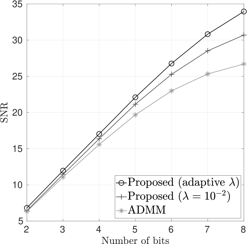
(b) Quantization

Figure 2: Comparison of the proposed consistent sparse coding algorithms using the $\ell_{1}$-norm, versus solving the constrained problem with ADMM.

cpu time (s)	Alg. 2	Alg. 1	ADMM
declipping	1.08	2.75	281.7
dequantization	1.19	2.91	320.3

TABLE I: Average computational time of each algorithm

VI-B Consistent dictionary learning

TABLE II: Performance of consistent dictionary learning on 1-bit recovery

Angular SNR (dB)	Classical	Classical	Consistent sparse coding (DCT)	Consistent dictionary learning
	sparse coding (DCT)	dictionary learning	(Algorithm 1)	(Algorithm 3)
Female speech	5.69	5.50	5.91	6.12
Male speech	4.67	4.47	4.50	4.70

We evaluate the proposed consistent dictionary learning algorithm on real speech signals. The dataset consists of 10 male and female speech signals, taken from the SISEC dataset [56]. Each signal is 10s long, sampled at 16kHz, with 16 bits per sample. Each signal is normalized to unit $\ell_{\infty}$ norm, and then processed using overlapping time frames of size $N=256$, with rectangular windows and 75% overlap, for a total of approximately $T=2500$ frames per signal. All sparse coding experiments are run using an overcomplete DCT dictionary of size $M=512$. All dictionary learning algorithms are initialized using the same DCT dictionary. To speed up convergence, the sparse coefficients and dictionaries are initialized at every iteration using the estimates from the previous iteration. Similarly, the step size parameters $\mu_{1}$ and $\mu_{2}$ can be re-estimated at every iteration as $\mu_{1}=1/\|{\mathbf{D}}\|_{2}^{2}$ and $\mu_{2}=1/\|{\mathbf{A}}\|_{2}^{2}$ using the current estimates of ${\mathbf{D}}$ and ${\mathbf{A}}$.

Figure 3 shows the performance of the proposed framework for consistent sparse coding and dictionary learning, compared to classical linear sparse coding and dictionary learning. In the case of declipping, the classical approach is to discard the clipped samples and treat declipping as an inpainting problem [4]. In the quantization case, the classical approach is to treat the quantized signals as noisy signals with variance $\frac{\Delta^{2}}{12}$ [19], which is enforced by stopping the algorithm when an error $\epsilon=\frac{\Delta^{2}}{12}$ is reached. For 1-bit signals, we simply use the sign measurements directly as the input [19]. All algorithms are run with an $\ell_{0}$-constraint with fixed $K=32$. In all three cases classical sparse coding is run using IHT [33], and classical dictionary learning alternates between IHT to update the sparse coefficients and gradient descent to update the dictionary. We perform 50 iterations for the sparse coding algorithms, and 50 iterations (with 20 iterations at each inner step) for dictionary learning.

Figure 3(a) shows the declipping performance, for different clipping levels ranging from $\theta=0.1$ (highly clipped) to $\theta=1$ (unclipped). Figure 3(a) demonstrates several things: First, using measurement consistency greatly improves the reconstruction. Consistent sparse coding shows an improvement of up to 8dB compared to classical sparse coding. Consistent dictionary learning shows up to 10dB improvement compared to classical dictionary learning. This improvement is greater when the signals are highly distorted ($\theta\leq 0.5$). As expected, the two frameworks give equivalent results when $\theta=1$, which shows how the proposed consistent framework naturally extends classical sparse coding. Second, we can see that consistent dictionary learning greatly improves the reconstruction performance compared to using a fixed DCT dictionary, since it adapts the dictionary to the signals of interest. This shows that the learned dictionary, although it has been learned using only the low-energy unclipped samples, along with consistency penalties, generalizes well to the unobserved clipped samples. In particular, the proposed consistent dictionary learning algorithm outperforms all the other methods. Finally, it is interesting to point out that when the signals are highly clipped ($\theta=0.1)$, classical dictionary learning does not improve compared to classical sparse coding with DCT. This is probably due to a lack of data to learn from, since most of the data is clipped and discarded. Our consistent dictionary learning algorithm on the other hand, makes use of the clipped data, and is able to learn and improve the performance by 1.7dB.

Figure 3(b) shows the results for quantization, from highly quantized ($N_{b}=2$ bits) to lightly quantized ($N_{b}=8$). Similarly, we can see that using measurement consistency improves the performance when the signals are heavily quantized $N_{b}\leq 5$. As expected, the performance of the consistent framework and of the classical one are comparable when the signals are lightly distorted ($N_{b}=8$). Dictionary learning improves the performance (compared to using a fixed dictionary), and the proposed consistent dictionary learning algorithm outperforms the other methods.

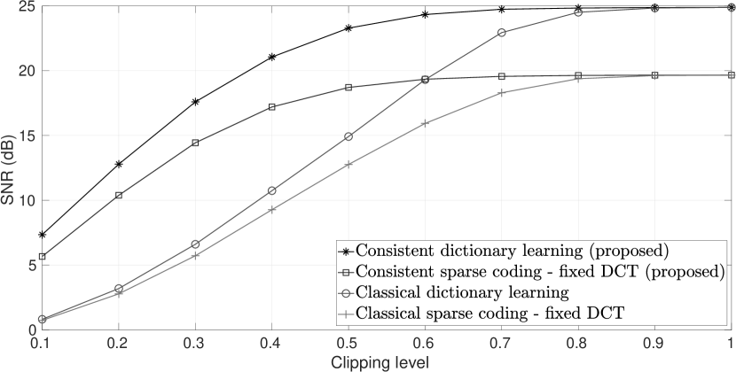
(a) Declipping

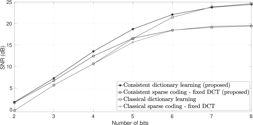
(b) De-quantization

Figure 3: Comparison of the proposed consistent sparse coding and dictionary learning algorithms, compared to classical sparse coding and dictionary learning.

The results for 1-bit data are shown in Table II. The results for sparse coding and consistent sparse coding are comparable (note that here for simplicity we don’t enforce the signal to be on the unit circle, unlike in [16, 19]). Classical dictionary learning here performs worse than classical sparse coding with a fixed dictionary, presumably because the reconstructed signal overfits the $\pm 1$ sign measurements. This shows that classical dictionary learning does not perform well with 1-bit data. The proposed consistent dictionary learning however, outperforms consistent sparse coding and classical dictionary learning.

VII Conclusion

We have presented a unified framework for signal reconstruction from certain types of nonlinear measurements such as clipping, quantization and 1-bit measurements. We proposed a cost function that takes into account prior knowledge about the measurement process, by minimizing the distance to the pre-image of the received signal. When the pre-image is convex, we have shown that the proposed cost is a convex, smooth and Lipschitz differentiable, which makes it ideal for proximal-based algorithms. The proposed cost generalizes the linear least-squares commonly used in sparse coding and dictionary learning, as well as cost functions proposed for declipping and 1-bit recovery. We proposed proximal based sparse coding and dictionary learning algorithms, which naturally extend classical algorithms and can deal with clipped, quantized and 1-bit measurements.

Appendix A Projection Theorem

We recall the following theorem [46, Prop. B.11]:

Theorem 1 (Projection Theorem [46, Prop. B.11]).

Let $\mathcal{C}$ be a closed convex set in $\mathbb{R}^{N}$. Then, the following hold:

a) For every ${\mathbf{x}}\in\mathbb{R}^{N}$, there exists a unique ${\mathbf{z}}^{*}\in\mathcal{C}$ such that ${\mathbf{z}}^{*}$ minimizes $\|{\mathbf{x}}-{\mathbf{z}}\|_{2}$ over all ${\mathbf{z}}\in\mathcal{C}$. ${\mathbf{z}}^{*}$ is called the projection of ${\mathbf{x}}$ onto $\mathcal{C}$ and is noted $\Pi_{\mathcal{C}}({\mathbf{x}})$. In other words:

$$\Pi_{\mathcal{C}}({\mathbf{x}})\triangleq\operatorname*{argmin}_{{\mathbf{z}}\in\mathcal{C}}\|{\mathbf{x}}-{\mathbf{z}}\|_{2}.$$ (44)

b) For ${\mathbf{x}}\in\mathbb{R}^{N}$, ${\mathbf{z}}^{*}=\Pi_{\mathcal{C}}({\mathbf{x}})$ if and only if:

$$({\mathbf{z}}-{\mathbf{z}}^{*})^{T}({\mathbf{x}}-{\mathbf{z}}^{*})\leq 0\quad\forall{\mathbf{z}}\in\mathcal{C}.$$ (45)

c) ${\mathbf{x}}\mapsto\Pi_{\mathcal{C}}({\mathbf{x}})$ is continuous and non-expansive, i.e:

$$\|\Pi_{\mathcal{C}}({\mathbf{x}}_{1})-\Pi_{\mathcal{C}}({\mathbf{x}}_{2})\|_{2}\leq\|{\mathbf{x}}_{1}-{\mathbf{x}}_{2}\|_{2}\quad\forall{\mathbf{x}}_{1},{\mathbf{x}}_{2}\in\mathbb{R}^{N}.$$ (46)

Appendix B Danskin’s Min-Max Theorem

Theorem 2 (Danskin’s Min-Max Theorem [57, Section 4.1], [29]).

Let $\mathcal{C}$ be a compact set, and $g({\mathbf{x}})=\min_{{\mathbf{z}}\in\mathcal{C}}\phi({\mathbf{x}},{\mathbf{z}})$. Suppose that for each ${\mathbf{z}}\in\mathbb{R}^{N}$, $\phi(\cdot,{\mathbf{z}})$ is differentiable with gradient $\nabla_{{\mathbf{x}}}\phi({\mathbf{x}},{\mathbf{z}})$, and $\phi({\mathbf{x}},{\mathbf{z}})$ and $\nabla_{{\mathbf{x}}}\phi({\mathbf{x}},{\mathbf{z}})$ are continuous on $\mathbb{R}^{N}\times\mathbb{R}^{N}$. Define $\mathcal{Z}({\mathbf{x}})=\operatorname*{argmin}_{{\mathbf{z}}\in\mathcal{C}}\phi({\mathbf{x}},{\mathbf{z}})$. Then $g$ is directionally differentiable, with derivative in the direction $\mathbf{h}$:

$$\nabla g({\mathbf{x}};\mathbf{h})=\min_{{\mathbf{z}}\in\mathcal{Z}({\mathbf{x}})}\nabla_{{\mathbf{x}}}\phi({\mathbf{x}},{\mathbf{z}})^{T}\mathbf{h}\quad\forall\mathbf{h},$$ (47)

In particular, when the minimum is attained at a unique point ($\mathcal{Z}({\mathbf{x}})=\{{\mathbf{z}}^{*}\}$), $g$ is differentiable with gradient:

$$\nabla g({\mathbf{x}})=\nabla_{{\mathbf{x}}}\phi({\mathbf{x}},{\mathbf{z}}^{*}).$$ (48)

In other words, Danskin’s Min-Max theorem says that if the minimum over a family of continuous and continuously differentiable functions is attained at a unique point ${\mathbf{z}}^{*}$, then the gradient of the minimum over this family of functions can be computed by simply evaluating that gradient at the optimum ${\mathbf{z}}^{*}$.

Appendix C Proofs of Proposition 1-3 and 5

Proof of Proposition 1:.

$\mathcal{L}_{f}(\cdot,\mathbf{y})$ is a minimum of a family of convex functions $({\mathbf{x}},{\mathbf{z}})\mapsto\frac{1}{2}\|{\mathbf{x}}-{\mathbf{z}}\|_{2}^{2}$ over a non-empty convex set, so by [58, Section 3.2.5], $\mathcal{L}_{f}(\cdot,\mathbf{y})$ is convex. ∎

Proof of Proposition 2:.

$\mathcal{L}_{f}({\mathbf{x}},\mathbf{y})=\min_{{\mathbf{z}}\in f^{-1}\{\mathbf{y}\}}\operatorname*{d}({\mathbf{x}},{\mathbf{z}})$ with $\operatorname*{d}({\mathbf{x}},{\mathbf{z}})=\frac{1}{2}\|{\mathbf{x}}-{\mathbf{z}}\|_{2}^{2}$. For all ${\mathbf{z}}\in\mathbb{R}^{N},\operatorname*{d}(\cdot,{\mathbf{z}})$ is differentiable with gradient $\nabla_{{\mathbf{x}}}\operatorname*{d}({\mathbf{x}},{\mathbf{z}})={\mathbf{x}}-{\mathbf{z}}$. Furthermore, $\operatorname*{d}({\mathbf{x}},{\mathbf{z}})$ and $\nabla_{{\mathbf{x}}}\operatorname*{d}({\mathbf{x}},{\mathbf{z}})$ are continuous in $({\mathbf{x}},{\mathbf{z}})$, and $\mathcal{Z}({\mathbf{x}})=\operatorname*{argmin}_{{\mathbf{z}}\in f^{-1}\{\mathbf{y}\}}\operatorname*{d}({\mathbf{x}},{\mathbf{z}})$ is uniquely defined as $\mathcal{Z}({\mathbf{x}})=\{\Pi_{f^{-1}\{\mathbf{y}\}}({\mathbf{x}})\}$ by the Projection Theorem. Using Danskin’s Min-Max theorem, we can then conclude that:

$$\begin{split}\nabla_{\mathbf{x}}\mathcal{L}_{f}({\mathbf{x}},\mathbf{y})=&\nabla_{{\mathbf{x}}}\operatorname*{d}({\mathbf{x}},\Pi_{f^{-1}\{\mathbf{y}\}}({\mathbf{x}}))\\ =&{\mathbf{x}}-\Pi_{f^{-1}\{\mathbf{y}\}}({\mathbf{x}}).\end{split}$$ (49)

∎

Proof of Proposition 3:.

Let ${\mathbf{x}}_{1},{\mathbf{x}}_{2}\in{\mathbb{R}}^{N}$. By the projection theorem, we have:

$$\begin{split}(\Pi_{f^{-1}\{\mathbf{y}\}}({\mathbf{x}}_{2})-\Pi_{f^{-1}\{\mathbf{y}\}}({\mathbf{x}}_{1}))^{T}({\mathbf{x}}_{1}-\Pi_{f^{-1}\{\mathbf{y}\}}({\mathbf{x}}_{1}))&\leq 0\\ (\Pi_{f^{-1}\{\mathbf{y}\}}({\mathbf{x}}_{1})-\Pi_{f^{-1}\{\mathbf{y}\}}({\mathbf{x}}_{2}))^{T}({\mathbf{x}}_{2}-\Pi_{f^{-1}\{\mathbf{y}\}}({\mathbf{x}}_{2}))&\leq 0.\end{split}$$ (50)

Adding and rearranging these two equations gives:

$$\begin{split}\|\Pi_{f^{-1}\{\mathbf{y}\}}(&{\mathbf{x}}_{1})-\Pi_{f^{-1}\{\mathbf{y}\}}({\mathbf{x}}_{2})\|_{2}^{2}\\ \leq&(\Pi_{f^{-1}\{\mathbf{y}\}}({\mathbf{x}}_{1})-\Pi_{f^{-1}\{\mathbf{y}\}}({\mathbf{x}}_{2}))^{T}({\mathbf{x}}_{1}-{\mathbf{x}}_{2}).\end{split}$$ (51)

We can then show that:

$$\begin{split}\|&\nabla_{{\mathbf{x}}}\mathcal{L}_{f}({\mathbf{x}}_{1},\mathbf{y})-\nabla_{{\mathbf{x}}}\mathcal{L}_{f}({\mathbf{x}}_{2},\mathbf{y})\|^{2}_{2}\\ &=\|{\mathbf{x}}_{1}-\Pi_{f^{-1}\{\mathbf{y}\}}({\mathbf{x}}_{1})-({\mathbf{x}}_{2}-\Pi_{f^{-1}\{\mathbf{y}\}}({\mathbf{x}}_{2}))\|^{2}_{2}\\ &=\|{\mathbf{x}}_{1}-{\mathbf{x}}_{2}\|^{2}_{2}+\|\Pi_{f^{-1}\{\mathbf{y}\}}({\mathbf{x}}_{1})-\Pi_{f^{-1}\{\mathbf{y}\}}({\mathbf{x}}_{2})\|^{2}_{2}\\ &\qquad-2({\mathbf{x}}_{1}-{\mathbf{x}}_{2})^{T}(\Pi_{f^{-1}\{\mathbf{y}\}}({\mathbf{x}}_{1})-\Pi_{f^{-1}\{\mathbf{y}\}}({\mathbf{x}}_{2}))\\ &\leq\|{\mathbf{x}}_{1}-{\mathbf{x}}_{2}\|^{2}_{2}-\|\Pi_{f^{-1}\{\mathbf{y}\}}({\mathbf{x}}_{1})-\Pi_{f^{-1}\{\mathbf{y}\}}({\mathbf{x}}_{2})\|^{2}_{2}\\ &\leq\|{\mathbf{x}}_{1}-{\mathbf{x}}_{2}\|_{2}^{2}\end{split}$$ (52)

where we have used (51) in the third line. ∎

Proof of Proposition 5.

The proof is given assuming exact estimation of the $\operatorname{\bm{\alpha}}^{k}$ coefficients, however similar results for approximate estimates are also available [46]. We have by definition of $\operatorname{\bm{\alpha}}^{k}$ and $\operatorname{\bm{\alpha}}^{k+1}$:

$$\begin{cases}&F(\lambda^{k+1},\operatorname{\bm{\alpha}}^{k+1})\leq F(\lambda^{k+1},\operatorname{\bm{\alpha}}^{k})\\ &F(\lambda^{k},\operatorname{\bm{\alpha}}^{k})\leq F(\lambda^{k},\operatorname{\bm{\alpha}}^{k+1})\end{cases}$$ (53)

Summing and rearranging these two equations gives:

$$(\lambda^{k+1}-\lambda^{k})(\Psi(\operatorname{\bm{\alpha}}^{k+1})-\Psi(\operatorname{\bm{\alpha}}^{k}))\leq 0,$$ (54)

Since $\lambda^{k+1}<\lambda^{k}$, we have $\Psi(\operatorname{\bm{\alpha}}^{k+1})\geq\Psi(\operatorname{\bm{\alpha}}^{k})$, from which follows (by combining with e.g., the first line of (53)) $\mathcal{L}_{f}({\mathbf{D}}\operatorname{\bm{\alpha}}^{k+1},\mathbf{y})\leq\mathcal{L}_{f}({\mathbf{D}}\operatorname{\bm{\alpha}}^{k},\mathbf{y})$.

We have furthermore that:

$$\min_{\operatorname{\bm{\alpha}}}F(\lambda^{k},\operatorname{\bm{\alpha}})\leq\min_{{\mathbf{D}}\operatorname{\bm{\alpha}}\in f^{-1}\{\mathbf{y}\}}F(\lambda^{k},\operatorname{\bm{\alpha}})=\lambda^{k}\Psi^{*}$$ (55)

Where $\Psi^{*}$ is the optimum value of (22). In other words:

$$0\leq\mathcal{L}_{f}({\mathbf{D}}\operatorname{\bm{\alpha}}^{k},\mathbf{y})+\lambda^{k}\Psi(\operatorname{\bm{\alpha}}^{k})\leq\lambda^{k}\Psi^{*}$$ (56)

When $\{\lambda^{k}\}\rightarrow 0$, taking the limit in (56) shows that $\lim_{k}\mathcal{L}_{f}({\mathbf{D}}\operatorname{\bm{\alpha}}^{k},\mathbf{y})=0$ and $\lim_{k}\Psi(\operatorname{\bm{\alpha}}^{k})\leq\Psi^{*}$. In particular, $F(\lambda^{k},\operatorname{\bm{\alpha}}^{k})$ converges to the optimum value $\Psi^{*}$ of the constrained problem (22). ∎

References

- [1] M. Elad and M. Aharon, “Image denoising via sparse and redundant representations over learned dictionaries,” IEEE Trans. Image Process., vol. 15, no. 12, pp. 3736–3745, 2006.
- [2] J. Mairal, M. Elad, and G. Sapiro, “Sparse representation for color image restoration,” IEEE Transactions on Image Processing, vol. 17, no. 1, pp. 53–69, 2008.
- [3] M. Elad, J.-L. Starck, P. Querre, and D. L. Donoho, “Simultaneous cartoon and texture image inpainting using morphological component analysis (MCA),” Appl. Computat. Harmon. Anal., vol. 19, no. 3, pp. 340–358, 2005.
- [4] A. Adler, V. Emiya, M. Jafari, M. Elad, R. Gribonval, and M. D. Plumbley, “Audio inpainting,” IEEE Trans. Audio, Speech, Language Process., vol. 20, no. 3, pp. 922–932, 2012.
- [5] J. Yang, J. Wright, T. S. Huang, and Y. Ma, “Image super-resolution via sparse representation,” IEEE Transactions on Image Processing, vol. 19, no. 11, pp. 2861–2873, 2010.
- [6] J. Yang, Z. Wang, Z. Lin, S. Cohen, and T. Huang, “Coupled dictionary training for image super-resolution,” IEEE Trans. Image Process., vol. 21, no. 8, pp. 3467–3478, 2012.
- [7] H. Mansour, R. Saab, P. Nasiopoulos, and R. Ward, “Color image desaturation using sparse reconstruction,” in Proc. IEEE Int. Conf. Acoust., Speech, Signal Process., 2010, pp. 778–781.
- [8] J. N. Laska, P. T. Boufounos, M. A. Davenport, and R. G. Baraniuk, “Democracy in action: Quantization, saturation, and compressive sensing,” Appl. Computat. Harmon. Anal., vol. 31, no. 3, pp. 429–443, 2011.
- [9] A. Adler, V. Emiya, M. G. Jafari, M. Elad, R. Gribonval, and M. D. Plumbley, “A constrained matching pursuit approach to audio declipping,” in Proc. IEEE Int. Conf. Acoust., Speech, Signal Process., 2011, pp. 329–332.
- [10] S. Kitić, L. Jacques, N. Madhu, M. P. Hopwood, A. Spriet, and C. D. Vleeschouwer, “Consistent iterative hard thresholding for signal declipping,” in Proc. IEEE Int. Conf. Acoust., Speech, Signal Process., May 2013, pp. 5939–5943.
- [11] B. Defraene, N. Mansour, S. D. Hertogh, T. van Waterschoot, M. Diehl, and M. Moonen, “Declipping of audio signals using perceptual compressed sensing,” IEEE Trans. Audio, Speech, Language Process., vol. 21, no. 12, pp. 2627–2637, Dec. 2013.
- [12] K. Siedenburg, M. Kowalski, and M. Dörfler, “Audio declipping with social sparsity,” in Proc. IEEE Int. Conf. Acoust., Speech, Signal Process., Florence, Italy, May 2014, pp. 1577–1578.
- [13] S. Kitić, N. Bertin, and R. Gribonval, “Sparsity and cosparsity for audio declipping: a flexible non-convex approach,” in Proc. Int. Conf. on Latent Variable Analysis and Signal Separation (LVA/ICA), Liberec, Czech Republic, 2015, pp. 243–250.
- [14] S. Foucart and T. Needham, “Sparse recovery from saturated measurements,” Information and Inference: A Journal of the IMA, vol. 6, no. 2, pp. 196–212, 2016.
- [15] R. M. Gray and D. L. Neuhoff, “Quantization,” IEEE Transactions on Information Theory, vol. 44, no. 6, pp. 2325–2383, 1998.
- [16] P. T. Boufounos and R. G. Baraniuk, “1-bit compressive sensing,” in 42nd Annual Conference on Information Sciences and Systems, 2008, pp. 16–21.
- [17] J. N. Laska, P. Boufounos, and R. G. Baraniuk, “Finite range scalar quantization for compressive sensing,” in Proc. Sampling Theory and Applications (SampTA), 2009.
- [18] E. J. Candes and T. Tao, “Near-optimal signal recovery from random projections: Universal encoding strategies?” IEEE Transactions on Information Theory, vol. 52, no. 12, pp. 5406–5425, 2006.
- [19] P. T. Boufounos, “Greedy sparse signal reconstruction from sign measurements,” in Conference Record of the Forty-Third Asilomar Conference on Signals, Systems and Computers, 2009, pp. 1305–1309.
- [20] W. Dai, H. V. Pham, and O. Milenkovic, “Distortion-rate functions for quantized compressive sensing,” in IEEE Information Theory Workshop on Networking and Information Theory, 2009, pp. 171–175.
- [21] A. Zymnis, S. Boyd, and E. Candès, “Compressed sensing with quantized measurements,” IEEE Signal Processing Letters, vol. 17, no. 2, pp. 149–152, 2010.
- [22] L. Jacques, D. K. Hammond, and J. M. Fadili, “Dequantizing compressed sensing: When oversampling and non-gaussian constraints combine,” IEEE Transactions on Information Theory, vol. 57, no. 1, pp. 559–571, 2011.
- [23] L. Jacques, K. Degraux, and C. De Vleeschouwer, “Quantized iterative hard thresholding: Bridging 1-bit and high-resolution quantized compressed sensing,” in Proc. 10th Int. Conf. Sampling Theory Appl. (SampTA), 2013.
- [24] A. Moshtaghpour, L. Jacques, V. Cambareri, K. Degraux, and C. De Vleeschouwer, “Consistent basis pursuit for signal and matrix estimates in quantized compressed sensing,” IEEE Signal Processing Letters, vol. 23, no. 1, pp. 25–29, 2016.
- [25] L. Jacques, J. N. Laska, P. T. Boufounos, and R. G. Baraniuk, “Robust 1-bit compressive sensing via binary stable embeddings of sparse vectors,” IEEE Transactions on Information Theory, vol. 59, no. 4, pp. 2082–2102, 2013.
- [26] P. Boufounos, M. F. Duarte, and R. G. Baraniuk, “Sparse signal reconstruction from noisy compressive measurements using cross validation,” in 2007 IEEE/SP 14th Workshop on Statistical Signal Processing (SSP 2007), 2007, pp. 299–303.
- [27] F. Couzinie-Devy, J. Mairal, F. Bach, and J. Ponce, “Dictionary learning for deblurring and digital zoom,” preprint arXiv:1110.0957, 2011.
- [28] J. Mairal, F. Bach, and J. Ponce, “Sparse modeling for image and vision processing,” Found. Trends Comput. Graph. Vis., vol. 8, no. 2-3, pp. 85–283, 2014.
- [29] J. M. Danskin, The theory of max-min and its application to weapons allocation problems. Ökonometrie und Unternehmensforschung, 1967.
- [30] P. Smaragdis, “Dynamic range extension using interleaved gains,” IEEE transactions on audio, speech, and language processing, vol. 17, no. 5, pp. 966–973, 2009.
- [31] S. Boyd, N. Parikh, E. Chu, B. Peleato, and J. Eckstein, “Distributed optimization and statistical learning via the alternating direction method of multipliers,” Foundations and Trends in Machine Learning, vol. 3, no. 1, pp. 1–122, 2011.
- [32] P. Zaviska, P. Rajmic, Z. Prusa, and V. Vesely, “Revisiting synthesis model in sparse audio declipper,” in International Conference on Latent Variable Analysis and Signal Separation. Springer, 2018, pp. 429–445.
- [33] T. Blumensath and M. E. Davies, “Iterative hard thresholding for compressed sensing,” Appl. Computat. Harmon. Anal., vol. 27, no. 3, pp. 265–274, 2009.
- [34] N. Parikh, S. P. Boyd et al., “Proximal algorithms,” Foundations and Trends in Optimization, vol. 1, no. 3, pp. 127–239, 2014.
- [35] K. Engan, S. O. Aase, and J. H. Husoy, “Method of optimal directions for frame design,” in Proc. IEEE Int. Conf. Acoust., Speech, Signal Process., vol. 5, 1999, pp. 2443–2446.
- [36] B. A. Olshausen and D. J. Field, “Sparse coding with an overcomplete basis set: A strategy employed by V1?” Vision Research, vol. 37, no. 23, pp. 3311–3325, 1997.
- [37] J. Mairal, F. Bach, J. Ponce, and G. Sapiro, “Online dictionary learning for sparse coding,” in Proc. Annual Int. Conf. Machine Learning, 2009, pp. 689–696.
- [38] W. Dai, T. Xu, and W. Wang, “Simultaneous codeword optimization (SimCO) for dictionary update and learning,” IEEE Transactions on Signal Processing, vol. 60, no. 12, pp. 6340–6353, 2012.
- [39] H. Zayyani, M. Korki, and F. Marvasti, “Dictionary learning for blind one bit compressed sensing,” IEEE Signal Processing Letters, vol. 23, no. 2, pp. 187–191, 2016.
- [40] Y. Shen and G. B. Giannakis, “Online dictionary learning from large-scale binary data,” in 24th European Signal Processing Conference (EUSIPCO), 2016, pp. 1808–1812.
- [41] L. Rencker, F. Bach, W. Wang, and M. D. Plumbley, “Consistent dictionary learning for signal declipping,” in Proc. Int. Conf. on Latent Variable Analysis and Signal Separation (LVA/ICA), Guildford, UK, 2018, pp. 446–455.
- [42] P. L. Combettes and J.-C. Pesquet, “Proximal splitting methods in signal processing,” in Fixed-point Algorithms for Inverse Problems in Science and Engineering. Springer, 2011, pp. 185–212.
- [43] A. Beck and M. Teboulle, “A fast iterative shrinkage-thresholding algorithm for linear inverse problems,” SIAM Journal on Imaging Sciences, vol. 2, no. 1, pp. 183–202, 2009.
- [44] D. M. Malioutov, M. Cetin, and A. S. Willsky, “Homotopy continuation for sparse signal representation,” in Proc. IEEE Int. Conf. Acoust., Speech, Signal Process., vol. 5. IEEE, 2005, pp. v–733.
- [45] B. Efron, T. Hastie, I. Johnstone, R. Tibshirani et al., “Least angle regression,” The Annals of statistics, vol. 32, no. 2, pp. 407–499, 2004.
- [46] D. P. Bertsekas, Nonlinear Programming, 2nd ed. Athena Scientific Belmont, 1999.
- [47] M. Aharon and M. Elad, “Sparse and redundant modeling of image content using an image-signature-dictionary,” SIAM Journal on Imaging Sciences, vol. 1, no. 3, pp. 228–247, 2008.
- [48] K. Kavukcuoglu and Y. Lecun, “Fast inference in sparse coding algorithms with applications to object recognition,” in Technical report, Computational and Biological Learning Lab, Courant Institute, NYU, 2008.
- [49] J. Mairal, F. Bach, J. Ponce, and G. Sapiro, “Online learning for matrix factorization and sparse coding,” Journal of Machine Learning Research, vol. 11, no. Jan, pp. 19–60, 2010.
- [50] D. Valsesia and P. T. Boufounos, “Universal encoding of multispectral images,” in 2016 IEEE International Conference on Acoustics, Speech and Signal Processing (ICASSP). IEEE, 2016, pp. 4453–4457.
- [51] F. Bach, R. Jenatton, J. Mairal, and G. Obozinski, “Convex optimization with sparsity-inducing norms,” Optimization for Machine Learning, vol. 5, 2011.
- [52] S. Bahmani, P. T. Boufounos, and B. Raj, “Robust 1-bit compressive sensing via gradient support pursuit,” arXiv preprint arXiv:1304.6627, 2013.
- [53] M. A. Davenport, Y. Plan, E. Van Den Berg, and M. Wootters, “1-bit matrix completion,” Information and Inference: A Journal of the IMA, vol. 3, no. 3, pp. 189–223, 2014.
- [54] W. Dai and O. Milenkovic, “Information theoretical and algorithmic approaches to quantized compressive sensing,” IEEE transactions on communications, vol. 59, no. 7, pp. 1857–1866, 2011.
- [55] N. T. Thao and M. Vetterli, “Set theoretic compression with an application to image coding,” IEEE transactions on image processing, vol. 7, no. 7, pp. 1051–1056, 1998.
- [56] A. Liutkus, F.-R. Stöter, Z. Rafii, D. Kitamura, B. Rivet, N. Ito, N. Ono, and J. Fontecave, “The 2016 signal separation evaluation campaign,” in International Conference on Latent Variable Analysis and Signal Separation. Springer, 2017, pp. 323–332.
- [57] J. F. Bonnans and A. Shapiro, “Optimization problems with perturbations: A guided tour,” SIAM Review, vol. 40, no. 2, pp. 228–264, 1998.
- [58] S. Boyd and L. Vandenberghe, Convex Optimization. Cambridge University Press, 2004.