MMT/MMIRS spectroscopy of $\mathbf{z=1.3-2.4}$ extreme [OIII] emitters: Implications for galaxies in the reionization-era

Abstract

Galaxies in the reionization-era have been shown to have prominent [O III]+H$\beta$ emission. Little is known about the gas conditions and radiation field of this population, making it challenging to interpret the spectra emerging at $z\gtrsim 6$. Motivated by this shortcoming, we have initiated a large MMT spectroscopic survey identifying rest-frame optical emission lines in 227 intense [O III] emitting galaxies at $1.3<z<2.4$. This sample complements the MOSDEF and KBSS surveys, extending to much lower stellar masses ($10^{7}-10^{8}M_{\odot}$) and larger specific star formation rates ($5-300$ Gyr^-1), providing a window on galaxies directly following a burst or recent upturn in star formation. The hydrogen ionizing production efficiency ($\xi_{\rm{ion}}$) is found to increase with the [O III] EW, in a manner similar to that found in local galaxies by Chevallard et al. (2018). We describe how this relationship helps explain the anomalous success rate in identifying Ly$\alpha$ emission in $z\gtrsim 7$ galaxies with strong [O III]+H$\beta$ emission. We probe the impact of the intense radiation field on the ISM using O32 and Ne3O2, two ionization-sensitive indices. Both are found to scale with the [O III] EW, revealing extreme ionization conditions not commonly seen in older and more massive galaxies. In the most intense line emitters, the indices have very large average values (O32 $=9.1$, Ne3O2 $=0.5$) that have been shown to be linked to ionizing photon escape. We discuss implications for the nature of galaxies most likely to have O32 values associated with significant LyC escape. Finally we consider the optimal strategy for JWST spectroscopic investigations of galaxies at $z\gtrsim 10$ where the strongest rest-frame optical lines are no longer visible with NIRSpec.

1 Introduction

Over the past decade, deep imaging surveys with the Hubble Space Telescope (HST) have uncovered thousands of color-selected galaxies at $z>6$ (e.g. McLure et al., 2013; Bouwens et al., 2015a; Finkelstein et al., 2015; Livermore et al., 2017; Atek et al., 2018; Oesch et al., 2018), revealing an abundant population of low mass systems that likely contribute greatly to the reionization of intergalactic hydrogen (Bouwens et al., 2015b; Robertson et al., 2015; Stanway et al., 2016; Dayal & Ferrara, 2018). These galaxies have been shown to be compact with low stellar masses, blue ultraviolet continuum slopes, and large specific star formation rates (see Stark 2016 for a review).

The James Webb Space Telescope (JWST) will eventually build on this physical picture, providing spectroscopic constraints on the stellar populations and gas conditions within the reionization era. Dedicated efforts throughout the last decade have delivered our first glimpse of what we are likely to see with JWST. Ground-based spectroscopic surveys have revealed a rapidly declining Ly$\alpha$ emitter fraction at $z>6$ (e.g. Caruana et al., 2014; Pentericci et al., 2014; Schenker et al., 2014), suggesting that the intergalactic medium (IGM) is likely partially neutral at $z\simeq 7-8$. While prominent Ly$\alpha$ emission is very rare in early galaxies, the rest-frame optical emission lines are found to be very strong relative to the underlying continuum, as expected for galaxies with large specific star formation rates (sSFR). The average [O III]+H$\beta$ equivalent width (EW) inferred from broadband flux excesses in stacked spectral energy distributions (SEDs) at $z\simeq 7-8$ is found to be $670$ Å (Labbé et al., 2013, hereafter L13), while individual objects have been located with combined [O III]+H$\beta$ equivalent widths reaching up to $1000-2000$ Å (Smit et al., 2014; Smit et al., 2015; Roberts-Borsani et al., 2016). While direct spectral measurements with JWST will ultimately be required to confirm the $z\sim 7$ equivalent width distribution, these measurements suggest large [O III] EWs ($>300$ Å) are likely to be very common.

These results indicate that the majority of reionization-era galaxies are caught in an extreme emission line phase, implying a large ratio of the flux density in the ionizing UV continuum ($\lambda<912$ Å) to that in the optical ($\lambda\simeq 4000-6000$ Å). There are a variety of ways a stellar population can produce such spectra. A likely pathway follows a recent upturn in the star formation rate (SFR), as would occur for systems undergoing rapidly rising star formation histories (which are expected at $z\gtrsim 6$; i.e. Behroozi et al. 2013) or punctuated bursts of star formation that greatly exceed earlier activity. In both cases, the stellar population will be dominated by recently formed stars, leading to an enhanced contribution from O stars relative to the longer-lived main-sequence stars that dominate the non-ionizing UV continuum and optical continuum. In this framework, the galaxies with the largest optical line equivalent widths (i.e., those approaching EW $=1000-2000$ Å) will be dominated by extremely hot massive stellar populations, resulting in an intense extreme UV (EUV) radiation field.

The interstellar gas reprocesses this radiation field, powering the observed nebular emission lines. Uncertainties in the form of the ionizing spectrum thus have a significant effect on the interpretation of the nebular spectrum. While the implementation of new physics in population synthesis models (i.e., stellar multiplicity, rotation) continues to improve predictions of the EUV radiation field (e.g. Levesque et al., 2012; Eldridge et al., 2017; Götberg et al., 2018), the shape of the ionizing spectrum between 1 and 4 Ryd remains very poorly constrained for a given age and metallicity. This is perhaps especially true among the highest equivalent width line emitters for which the EUV spectrum is extremely sensitive to the nature of the hottest and most massive stars present in the galaxy. While large spectroscopic surveys have begun to constrain the ionizing spectrum of typical galaxies at $z\simeq 2-3$ (e.g. Sanders et al., 2016; Steidel et al., 2016; Strom et al., 2017), much less work has focused on the extreme emission line population.

As the first nebular spectra of $z\gtrsim 6$ galaxies emerge, we are already beginning to see indications that the ionizing spectra of reionization-era sources differ greatly from typical galaxies at lower redshifts. Perhaps most surprising has been the detection of strong nebular C IV emission in two of the first galaxies observed at $z\gtrsim 6$ (Stark et al., 2015b; Mainali et al., 2017; Schmidt et al., 2017), implying a very hard EUV ionizing spectrum capable of triply ionizing carbon in the ISM. The presence of C IV in a high redshift galaxy typically indicates the power law spectrum of an active galactic nucleus (AGN). However, Mainali et al. (2017) have demonstrated that the observed line ratios in one of the $z>6$ C IV emitters requires a strong break at the He⁺-ionizing edge, suggesting a metal poor ($<0.1\ Z_{\odot}$) stellar ionizing spectrum is likely responsible for powering the nebular emission. The precise form of the EUV spectrum produced by massive stars in this metallicity regime is very uncertain, making it difficult to reliably link the observed nebular emission to a unique physical picture. Similar challenges have emerged following detections of intense C III] emission in two galaxies at $z\gtrsim 6$ (Stark et al., 2015a, 2017). Whereas some have argued that the UV line emission can be powered by moderately metal poor, young stellar populations (Stark et al., 2017), others suggest an AGN contribution is necessary to explain the large C III] equivalent width (Nakajima et al., 2018). Until more is known about the EUV radiation field of very young stellar populations that dominate in extreme emission line galaxies (EELGs), it will be difficult to reliably interpret the the $z\gtrsim 6$ nebular line spectra that will be common in the JWST era.

The uncertainties in the EUV spectra of early galaxies also plague efforts to use Ly$\alpha$ as a probe of reionization. The success of the Ly$\alpha$ reionization test hinges on our ability to isolate the impact of the IGM on the evolving Ly$\alpha$ equivalent width distribution, requiring careful attention to variations in the intrinsic production of Ly$\alpha$ within the galaxy population. The intrinsic Ly$\alpha$ luminosity of a given stellar population (per SFR) depends sensitively on the production efficiency of Lyman continuum (LyC) radiation (e.g. Wilkins et al., 2016), often parameterized as $\xi_{\rm{ion}}=N(\rm{H}^{0})/L_{\rm{UV}}$, the ratio of production rate of hydrogen ionizing photons ($N(\rm{H}^{0})$) and the continuum luminosity of non-ionizing UV photons ($L_{\rm{UV}}$). By definition, the extreme emission line galaxies that dominate in the reionization era should be extraordinarily efficient at producing hydrogen ionizing radiation. Efforts to measure $\xi_{\rm{ion}}$ from both high quality spectra (e.g. Chevallard et al., 2018; Shivaei et al., 2018) and narrowband imaging (Matthee et al., 2017) have ramped up in recent years. Chevallard et al. (2018) demonstrated a correlation exists between $\xi_{\rm{ion}}$ and [O III] EW among ten nearby galaxies, such that the most extreme line emitters are the most efficient in their ionizing photon production. The first hints at high redshift suggest a similar picture (Matthee et al., 2017; Shivaei et al., 2018), but the LyC production efficiency of extreme emission line galaxies remains poorly constrained. As a result, it is not known the extent to which $\xi_{\rm{ion}}$ varies over the full range of equivalent widths present in reionization era galaxies (EW${}_{\rm{[OIII]+H}\beta}\simeq 300-2000$ Å), making it challenging to accurately account for how variations in the radiation field are likely to impact Ly$\alpha$ visibility.

The limitations of our physical picture of Ly$\alpha$ production in the reionization era has recently become apparent following the discovery of four massive $z\simeq 7-9$ galaxies with extremely large [O III]+H$\beta$ equivalent widths (EW${}_{\rm{[OIII]+H}\beta}\simeq 1000-2000$ Å; Roberts-Borsani et al. 2016, hereafter RB16). Spectroscopic follow-up has revealed Ly$\alpha$ in each of the four galaxies from RB16 (e.g. Oesch et al., 2015; Zitrin et al., 2015; Stark et al., 2017), corresponding to a factor of ten higher success rate than was found in earlier studies (e.g. Schenker et al., 2014; Pentericci et al., 2014). The association between Ly$\alpha$ and extreme EW [O III] emission is also seen in other $z>7$ Ly$\alpha$ emitters with robust IRAC photometry (Ono et al., 2012; Finkelstein et al., 2013). Remarkably these results suggest significant differences between the Ly$\alpha$ properties of the extreme line emitters that are typical at $z\gtrsim 7$ (EW${}_{\rm{[OIII]+H}\beta}\simeq 670$ Å) and massive systems with slightly larger equivalent widths (EW${}_{\rm{[OIII]+H}\beta}\simeq 1000-2000$ Å). This could imply that the transmission of Ly$\alpha$ is enhanced in the higher equivalent width sources, as might be expected if these massive galaxies trace larger-than-average ionized patches of the IGM. Or it could be explained if the production efficiency of Ly$\alpha$ is much larger in the higher EW sources. In this case, efforts to model the evolving Ly$\alpha$ EW distribution would have to control for the large intrinsic variations in the Ly$\alpha$ luminosity per SFR that accompany sources of slightly different [O III] EW. Unfortunately without robust measurements of how $\xi_{\rm{ion}}$ scales with [O III] EW at high redshift, it is impossible to know which picture is correct.

The shortcomings described above motivate the need for a comprehensive investigation of the spectral properties of high redshift extreme emission line galaxies. Prior to the launch of JWST, this is most easily accomplished at $z\simeq 2$ where both rest-UV and rest-frame optical nebular lines are visible from the ground. In this paper, we present the first results from a near-infrared spectroscopic survey targeting rest-frame optical nebular emission lines in over 200 extreme emission line galaxies at $z=1.3-2.4$. Our sample is selected using a combination of HST grism spectra (Brammer et al., 2012; Skelton et al., 2014; Momcheva et al., 2016) and broadband photometry. Over the past 2.5 years, we have obtained $\simeq 100$ hours of MMT and Keck spectroscopy following up this population in the near-infrared. The program is ongoing, and we ultimately aim to obtain useful constraints on the strongest rest-frame optical lines ([O II], [Ne III], H$\beta$, [O III], H$\alpha$, [N II]) for each galaxy in our sample. This program complements the KBSS (Steidel et al., 2014) and MOSDEF (Kriek et al., 2015) programs, including galaxies with lower masses and larger specific star formation rates than are common in these surveys.

We focus on three key topics in this paper. First we use our spectra to characterize how the production efficiency of LyC (and hence Ly$\alpha$) photons scales with the [O III] and H$\alpha$ EW. Using this information, we consider how variations in Ly$\alpha$ production efficiency impact the visibility of Ly$\alpha$ at $z>7$. Second, we investigate how the intense radiation field of extreme emission line galaxies impacts the conditions of the ISM, characterizing how rest-frame optical line ratios that are sensitive to the ionization state of the gas vary with [O III] EW. We discuss the findings in the context of results showing an association between ionization-sensitive line ratios and the escape fraction of ionization radiation. Third we use our emission line measurements to help optimize spectroscopic observations of the highest redshift galaxies ($z\gtrsim 10$) that JWST will target. At these redshifts, the strongest rest-frame optical lines ([O III], H$\alpha$) are no longer visible with NIRSpec. We consider whether fainter rest-frame optical lines (i.e., [O II], [Ne III]) will provide viable alternatives and make predictions for the range of equivalent widths that are likely to be present in early galaxies.

The organization of this paper is as follows. We describe the sample selection and near-infrared spectroscopic observations in §2. We introduce our photoionization modeling procedure in §3 before discussing the rest-frame optical spectroscopic properties of the EELGs in §4. We discuss the implications in §5, and summarize our results in §6. We adopt a $\Lambda$-dominated, flat Universe with $\Omega_{\Lambda}=0.7$, $\Omega_{M}=0.3$ and $\rm{H}_{0}=70$ km s^-1 Mpc^-1. All magnitudes in this paper are quoted in the AB system (Oke & Gunn, 1983), and all equivalent widths are quoted in the rest-frame. We assume a Chabrier (2003) initial mass function throughout the paper.

2 Observations and Analysis

We have initiated a large spectroscopic survey of $z\simeq 2$ galaxies with extremely large equivalent width optical emission lines. A complete description of the survey and the galaxies targeted will be presented in a catalog paper following the end of the survey. Here we provide a detailed summary of the survey and resulting emission line sample, describing the pre-selection of targets (§2.1) and our campaign to follow-up these sources with spectrographs on MMT and Keck (§2.2$-$2.4). We discuss the analysis of the spectra and our current redshift catalog in §2.5.

2.1 Pre-Selection of Extreme Emission Line Galaxies

The first step in our survey is to identify a robust sample of extreme emission line galaxies for spectroscopic follow-up. Since we aim to study how the radiation field and gas conditions vary within the reionization era population, we must select galaxies at that span the full range of equivalent widths expected at $z\gtrsim 6$ (EW${}_{\rm{[OIII]+H}\beta}\simeq 300-2000$ Å; e.g., Stark 2016). This pre-selection is most efficiently performed using publicly-available HST WFC3 G141 grism spectra in the five CANDELS (Grogin et al., 2011; Koekemoer et al., 2011) fields. The G141 grism covers between $1.1\ \mu$m and $1.7\ \mu$m, enabling identification of H$\alpha$ at $0.7<z<1.6$ and [O III]$\lambda\lambda 4959,5007$ (blended at the grism resolution) at $1.2<z<2.4$. Four of the fields (AEGIS, COSMOS, GOODS-S, UDS) have been targeted by the 3D-HST program (van Dokkum et al., 2011; Brammer et al., 2012; Skelton et al., 2014; Momcheva et al., 2016), and the fifth field (GOODS-N) was observed in GO-11600 (PI:Weiner). The latest 3D-HST public release brings together all the G141 data, providing photometry (Skelton et al., 2014) and spectral measurements (Momcheva et al., 2016) of galaxies in all five CANDELS fields.

Our primary selection is focused on systems in two redshift windows ($1.37\leq z\leq 1.70$, $2.09\leq z\leq 2.48$) where the full set of strong rest-frame optical lines ([O II], H$\beta$, [O III], H$\alpha$) can be observed with ground-based spectrographs. At $1.37\leq z\leq 1.70$, we can detect H$\beta$ and [O III] in the $J$ band, and H$\alpha$ in the $H$ band. [O II] is situated in the $Y$ band at $1.55\leq z\leq 1.70$ and in the optical at $z<1.55$. At $2.09\leq z\leq 2.48$, we can detect [O II] in the $J$ band, H$\beta$ and [O III] in the $H$ band, and H$\alpha$ in the $K$ band. We also identify secondary targets at $1.70<z<1.90$ and $2.02<z<2.09$, where a subset of the lines are visible using ground-based spectrographs. We will discuss the relative priorities we assign to galaxies when introducing the near-infrared spectroscopic follow-up in §2.2.

As a first pass at our pre-selection, we use the 3D-HST v.4.1.5 grism catalogs (see Momcheva et al. 2016) to select extreme line emitters in all five CANDELS fields. These catalogs include extracted grism spectra for objects with WFC3 F140W magnitude $<26.0$. We aim to select galaxies with optical line equivalent widths similar to those seen in the reionization era. Stacked broadband SEDs imply typical values of [O III]+H$\beta$ EW $=670$ Å at $z\simeq 8$ (L13). To ensure our sample spans the full range of line strengths seen at $z\simeq 8$, we consider all objects with [O III]+H$\beta$ EW $>340$ Å, roughly a factor of two below the average value quoted above. We thus select all galaxies in the grism catalogs with [O III]$\lambda\lambda 4959,5007$ EW $>300$ Å. Here we have assumed a flux ratio of [O III]$\lambda 5007$/H$\beta$ $=6$, consistent with measurements of extreme emission line galaxies at $z\simeq 2$ (Maseda et al., 2014). For the sake of simplicity, we use the same equivalent width threshold for H$\alpha$. The precise value we choose does not impact our results, as we will sample a wide range of equivalent widths in our follow-up survey. For reference, if we crossmatch the MOSDEF spectroscopic sample to the 3D-HST grism catalogs (considering only galaxies in same redshift range as in our EELG sample), we find that the median [O III]$\lambda\lambda 4959,5007$ EW is $154$ Å  for sources with S/N $>3$ grism line detections. Our sample thus largely probes a distinct [O III] EW regime.

The efficiency of our follow-up spectroscopy program depends sensitively on how accurately the equivalent widths can be measured from the grism spectra, requiring robust measurements of both the line flux and the underlying continuum. To ensure the line detections are robust, we only include sources with significant (S/N $>3$) [O III] or H$\alpha$ flux and equivalent width measurements. However we find that the equivalent width S/N threshold excises many extreme line emitters from our sample owing to the low S/N continuum in many of the grism spectra. For these fainter continuum sources, we can more reliably identify extreme line emitters using the line flux from the grism catalogs and the continuum from the HST broadband imaging data. We estimate the equivalent width errors for this subset by adding the uncertainties of emission line fluxes and broadband photometry in quadrature. If the rest-frame [O III]$\lambda\lambda 4959,5007$ or H$\alpha$ equivalent width calculated in this manner is above $300$ Å with S/N $>3$, we include the source in our catalog for follow-up spectroscopy.

Finally we visually inspect the grism spectra and photometry of all galaxies that satisfy these criteria, removing sources with grism spectra that are unreliable owing to contamination from overlapping spectra or those that appear to have misidentified emission lines. We are left with a sample of 1587 galaxies with grism measurements that imply [O III]$\lambda\lambda$4959,5007 or H$\alpha$ rest-frame EW greater than $300$ Å across the five CANDELS fields. Examples of the broadband SEDs of the extreme emission line galaxies in our sample are shown in Figure 1. In all cases, the measured flux in the specific broadband filters that sample the strong nebular emission lines are well above the flux of the underlying continuum.

The grism observations cover $\sim 75\%$ of the area imaged by the CANDELS survey. While our spectroscopic follow-up observations are centered in these regions, often the edges of the slitmasks extend to areas of the CANDELS fields that lack grism spectra. In these sub-regions, we use simple color cuts to identify extreme emission line galaxies based on the characteristic shape of their broadband SEDs. In the redshift range $1.6<z<1.8$, galaxies with large equivalent width [O III]+H$\beta$ emission show a large flux excess in the $J_{\rm{125}}$-band (Figure 1). Previous studies have successfully demonstrated that extreme [O III]+H$\beta$ emitters can be easily selected by identifying galaxies in which the $J_{\rm{125}}$-band flux is significantly greater than that in the $I$ and $H_{\rm{160}}$-bands (van der Wel et al., 2011; Maseda et al., 2014). We closely follow these selections, identifying galaxies in the Skelton et al. (2014) photometric catalogs that satisfy the following criteria: $I-J_{125}>0.3+\sigma(I-J_{125})$ and $J_{125}-H_{160}<-0.3-\sigma(J_{125}-H_{160})$, where $\sigma$ is the color uncertainty. The required $J$-band flux excess is chosen to match the equivalent width threshold of our grism sample. Whereas the grism selection identifies strong [O III]$\lambda\lambda$4959,5007 or H$\alpha$ emission, the photometric selection picks out sources based on their combined [O III]+H$\beta$ emission. Under the same assumptions described above, our color cuts correspond to a selection of galaxies at $1.6<z<1.8$ with [O III]+H$\beta$ EW $>340$ Å. We have verified (in fields where grism spectra are available) that this selection identifies the same extreme emission line galaxies selected via the grism catalogs.

Following Maseda et al. (2014), we also select [O III]+H$\beta$ emitter candidates at $2.0<z<2.4$ via an $H_{\rm{160}}$-band flux excess technique. Because of the limited $K$-band sensitivity, the color cuts identify sources in which $H_{160}$ is significantly in excess of $J_{125}$. To minimize contamination from Balmer break sources, Maseda et al. (2014) introduce a requirement that galaxies additionally have blue UV continuum (in $V-I$) slopes. We adopt similar color cuts, again making minor adjustments to the required color excess for the sake of consistency with our grism selection. In particular, we identify sources with $V_{606}-I<0.1-\sigma(V_{606}-I)$ and $J_{125}-H_{160}>0.36+\sigma(J_{125}-H_{160})$. We also require that the detections in $V_{606}$, $I$, $J_{125}$ and $H_{160}$ have S/N $>5$. The two color section techniques provide an additional 612 targets, resulting in a total sample of 2199 galaxies in our input catalog.

The final step is to remove galaxies that likely host AGNs from the sample. While recent studies of EELG at $z\gtrsim 7$ suggests that AGN may be present in several of the sources for which we are obtaining spectra (e.g. Tilvi et al., 2016; Laporte et al., 2017; Mainali et al., 2018), our goal is to focus first on the range of spectral properties in galaxies dominated by star formation. We use the deep Chandra X-ray imaging in AEGIS (Nandra et al., 2015), COSMOS (Civano et al., 2016), GOODS-N (Alexander et al., 2003; Xue et al., 2016), and GOODS-S (Xue et al., 2011) fields, as well as XMM X-ray imaging in UDS field (Ueda et al., 2008) to identify X-ray sources in the sample. We match the coordinates of our EELG candidates to the X-ray source catalogs using a $1\aas@@fstack{\prime\prime}0$ search radius. There are 26 sources in our sample found to have X-ray counterparts within $1\aas@@fstack{\prime\prime}0$. We remove these 26 sources, leaving 2173 targets in the final grism spectroscopy and photometry-selected EELG candidate sample.

Figure 1: Examples of the broadband SEDs of the extreme [O III] line emitting galaxies at $z=1.3-2.4$ in our sample. The upper panels show three of the sources with very large EWs in our sample ([O III]$\lambda 5007$ EW $>1000$ Å) that similar to the $z>7$ galaxies in RB16. The lower panels show three of the sources with equivalent widths slightly above the average EW of $z>7$ galaxies ([O III]$\lambda 5007$ EW $\simeq 450$ Å; L13). Observed broadband photometry is shown as solid black circles. The best-fitting SED models (inferred from BEAGLE, see §3) are plotted by solid blue lines, and synthetic photometry is shown as open green squares. Strong rest-frame optical emission lines, [O III]$\lambda 5007$ and H$\alpha$, are highlighted by dashed black lines. Spectroscopic redshift, object ID, and rest-frame [O III]$\lambda 5007$ EW are listed in each panel. The LyC photon production efficiency ($\xi^{\rm{HII}}_{\rm{ion}}$) and the ionization-sensitive line ratio [O III]/[O II] of each object are also listed.

2.2 MMT/MMIRS Spectroscopy

We use the catalog of extreme equivalent width line emitters described in §2.1 as input for our ground-based spectroscopic follow-up program, the majority of which is conducted at the MMT using the MMT and Magellan Infrared Spectrograph (MMIRS; McLeod et al. 2012). MMIRS is a wide-field near-infrared imager and multi-object spectrograph (MOS) with a field of view of $4^{\prime}\times 6^{\prime}.9$. We used the “xfitmask” software to design our MMIRS slit masks, using a slit length of $7\aas@@fstack{\prime\prime}0$ and a slit width of $1\aas@@fstack{\prime\prime}0$ for science targets. Data were obtained over six observing runs between the 2015B and 2018A semesters. Thus far, we have collected 81 hours of on-source integration with MMIRS, allowing us to target 313 galaxies on 17 separate masks, with 58 galaxies observed on two masks.

Our selection function is defined primarily by the redshift and equivalent width of the targets. We first prioritize galaxies at $1.37\leq z\leq 1.70$ and $2.09\leq z\leq 2.48$, where the full set of strong rest-frame optical emission lines can be obtained from ground-based observations. For galaxies at $1.37\leq z\leq 1.70$, we give the highest priority to those at $1.55\leq z\leq 1.70$, where all strong rest-frame optical lines can be probed by MMIRS observations. Galaxies at $z<1.55$ will need additional follow-up with red-sensitive optical spectrographs to detect the [O II] emission line. We next adjust the target priority in each redshift interval based on the grism equivalent width or the flux excess implied by photometry. Sources with the highest equivalent widths are extraordinarily rare, with only $15-20$ (3) galaxies per CANDELS field with [O III]$\lambda 5007$ EW $>1000\ (2000)$ Å. To ensure that our sample contains an adequate number (i.e., $5-10$) of the largest equivalent width galaxies, we increase the priority of objects with the largest equivalent widths in each redshift interval. This is the minimum number required for us to characterize the average line ratios in this [O III] EW range. Finally, we prioritize grism-selected targets over those identified by photometric excesses when both are available in the same region of a slitmask.

The details of the MMIRS masks obtained to date are summarized in Table 1. Spectra were taken with the J grism + zJ filter, H3000 grism + H filter, and K3000 grism + Kspec filter, providing wavelength coverage of $0.95-1.50\ \mu$m, $1.50-1.79\ \mu$m and $1.95-2.45\ \mu$m, respectively. The $1\aas@@fstack{\prime\prime}0$ slit widths result in resolving power of $R=960$, $1200$, and $1200$ for J + zJ, H3000 + H, and K3000 + Kspec grism and filter sets, respectively. The total integration time in each filter ranges from 1 hr to 8 hr, with the specific value chosen depending on the predicted brightness of the set of emission lines we are targeting. The average seeing was between $0\aas@@fstack{\prime\prime}6$ and $1\aas@@fstack{\prime\prime}6$ (see Table 1). The masks all contained an isolated star to monitor the throughput and seeing during the observations and to compute the absolute flux calibration. For each mask and filter combination, we also observed A0V stars at a similar airmass to derive the response spectrum and correct for telluric absorption.

We reduced our MMIRS data using the publicly available data reduction pipeline developed by the instrument team. The MMIRS data reduction pipeline is implemented in IDL and described in Chilingarian et al. (2015). Individual two-dimensional (2D) spectra are extracted from the original frames and flat-fielded after spectral tracing and optical distortion mapping. The wavelength calibration uses atmosphere airglow OH lines, or the internal argon arc lamp if the OH based computation fails. For sky subtraction, the pipeline creates a night sky spectrum model using science frames and the precise pixel-to-wavelength mapping, and subtracts the night sky emission from the 2D spectra. Finally, the pipeline provides telluric correction by first computing the atmosphere transmission curve (including spectral response function of the detector) from the observed telluric star spectra, and then correcting the transmission using a grid of atmospheric transmission models to account for the airmass difference between observations of the science target and the telluric star. The pipeline outputs the sky-subtracted and telluric-corrected 2D spectra of every slit on the mask.

One-dimensional (1D) spectra are then extracted from the fully-reduced 2D spectra. In cases where an emission line or continuum is detected with confidence, we use an optimal extraction procedure (Horne, 1986). In all other cases we use a simple boxcar extraction, with the extraction aperture matched to the object spatial profile. We have verified that the extraction method does not significantly impact on the line flux measurements. The absolute flux calibration is then applied to the extracted 1D spectra using the slit stars. Slit loss corrections are performed following the similar procedures in Kriek et al. (2015). We first extract a postage stamp of each galaxy from the HST F160W image (Skelton et al., 2014), then smooth the postage stamp and fit the smoothed image with a 2D Gaussian profile. We compute the fraction of the light within the slit to that of the total Gaussian profile. Each spectrum is multiplied by the ratio of the in-slit light fraction measured for the slit star to that for each galaxy.

Mask Name	Number of Target	R.A.	Decl.	P.A.	Grism	Filter	Exposure Time	Average Seeing
		(hh:mm:ss)	(dd:mm:ss)	(deg)			(seconds)	(′′)
(1)	(2)	(3)	(4)	(5)	(6)	(7)	(8)	(9)
udsel1	24	2:17:49.000	$-$5:13:02.00	$-$11.00	J	zJ	14400	1.2
udsel2	23	2:17:26.000	$-$5:13:20.00	$-$116.00	J	zJ	14400	0.8
udsel3	24	2:17:26.000	$-$5:12:13.00	88.00	J	zJ	28800	0.8
udsel3	24	2:17:26.000	$-$5:12:13.00	88.00	H3000	H	7200	0.8
egsel3	24	14:19:25.973	52:50:08.43	177.00	J	zJ	21000	0.6
egsel3	24	14:19:25.973	52:50:08.43	177.00	H3000	H	6000	1.0
egsel4	23	14:19:58.000	52:55:04.01	179.00	J	zJ	10200	0.8
egsel4	23	14:19:58.000	52:55:04.01	179.00	H3000	H	2400	1.0
gdnel3	27	12:37:14.173	62:19:29.10	$-$162.00	J	zJ	14400	0.8
gdnel3	27	12:37:14.173	62:19:29.10	$-$162.00	H3000	H	12000	1.2
gdnel4	23	12:36:31.204	62:14:51.55	$-$125.00	J	zJ	12000	0.8
gdnel4	23	12:36:31.204	62:14:51.55	$-$125.00	H3000	H	7200	0.8
udsel5	14	2:17:17.088	$-$5:14:53.13	$-$86.00	J	zJ	7200	1.2
udsel5	14	2:17:17.088	$-$5:14:53.13	$-$86.00	H3000	H	14400	1.2
udsel6	21	2:17:49.000	$-$5:13:02.00	106.00	J	zJ	7200	1.2
udsel6	21	2:17:49.000	$-$5:13:02.00	106.00	H3000	H	14400	1.6
egsel1	20	14:19:37.358	52:50:22.97	$-$179.00	J	zJ	14400	1.1
egsel1	20	14:19:37.358	52:50:22.97	$-$179.00	K3000	Kspec	3600	0.7
egsel2	19	14:20:07.295	52:54:13.13	$-$134.00	J	zJ	3600	0.6
egsel2	19	14:20:07.295	52:54:13.13	$-$134.00	K3000	Kspec	3600	1.6
gdnel5	22	12:37:08.882	62:19:36.39	$-$162.00	H3000	H	3600	0.8
gdnel5	22	12:37:08.882	62:19:36.39	$-$162.00	K3000	Kspec	3600	0.7
gdnel6	17	12:37:22.384	62:18:02.04	$-$143.00	J	zJ	7200	1.0
egsel5	15	14:20:11.119	52:56:50.92	120.00	J	zJ	7200	0.8
udsel7	27	2:17:15.656	$-$5:14:04.59	93.00	J	zJ	10800	0.8
udsel7	27	2:17:15.656	$-$5:14:04.59	93.00	K3000	Kspec	3600	0.8
udsel8	25	2:17:36.777	$-$5:11:40.87	$-$77.00	J	zJ	10800	0.8
udsel8	25	2:17:36.777	$-$5:11:40.87	$-$77.00	K3000	Kspec	3600	0.8
egsel6	23	14:19:15.000	52:46:29.00	$-$146.00	J	zJ	13200	1.0
egsel6	23	14:19:15.000	52:46:29.00	$-$146.00	H3000	H	7200	1.0
egsel6	23	14:19:15.000	52:46:29.00	$-$146.00	K3000	Kspec	3600	1.0

Table 1: Summary of MMT/MMIRS observations. Column (1): mask name; Column (2): number of science targets on each mask, alignment stars and slit stars are not included; Column (3): right ascension of the mask center; Column (4): declination of the mask center; Column (5): position angle of the mask; Column (6): grism of the mask observed; Column (7): filter of the mask observed; Column (8): Total exposure time of the mask in each grism + filter set; Column (9): average seeing during the observation, in full width at half maximum (FWHM).

2.3 Keck/MOSFIRE Spectroscopy

We also obtained spectra from the Multi-object Spectrometer for Infrared Exploration (MOSFIRE; McLean et al. 2012) on the Keck I telescope. We placed galaxies on masks using the same selection function described in §2.2. We used the MAGMA software to design the slit masks, and adopted a slit width of $0\aas@@fstack{\prime\prime}7$. Data were obtained on observing runs in 2015 November (one mask in the COSMOS field, one mask in the GOODS-S field, and one mask in the UDS field), and 2016 April (two masks in the AEGIS field). We have summarized the details of the Keck/MOSFIRE observations in Table 2. Spectra were taken in the Y, J, and H bands, providing wavelength coverage of $0.972-1.125\ \mu$m, $1.153-1.352\ \mu$m, and $1.468-1.804\ \mu$m. The slit width of $0\aas@@fstack{\prime\prime}7$ results in resolving power of $R=3388$, $3318$, and $3660$ for Y, J, and H, respectively. The total integration time for each mask in each band ranges from 0.5 hr to 4.3 hr. The average seeing during the observations was between $0\aas@@fstack{\prime\prime}46$ and $0\aas@@fstack{\prime\prime}94$. The masks all contained $1-2$ isolated stars to monitor the throughput and seeing. We use these stars to derive the absolute flux calibration. We also observed A0V stars in Y, J, and H bands to derive the response spectrum and correct for telluric absorption. In total, we observed 94 targets on 5 separate masks with MOSFIRE.

Our MOSFIRE data were reduced using the publicly available data reduction pipeline (DRP), which is implemented in PYTHON. The MOSFIRE DRP first generates a flat-fielded image and traces the slit edge for each mask. Using a median-combined image of all science exposures, wavelength solutions are fit interactively for the central pixel in each slit using the night sky OH emission lines, and propagated spatially along the slit. After wavelength calibration and background subtraction, the two A$-$B and B$-$A stacks are shifted, combined and rectified to produce the final 2D spectra. We derive the telluric correction spectra using longslit observations of a telluric standard star. The absolute flux scaling factors are computed by comparing the count rates of slit star spectra with the flux densities in the 3D-HST photometric catalogs. Slit loss corrections were applied following the procedures in Kriek et al. (2015) as described in §2.2.

Mask Name	Number of Targets	R.A.	Decl.	P.A.	Band	Exposure Time	Average Seeing
		(hh:mm:ss)	(dd:mm:ss)	(deg)		(seconds)	(′′)
(1)	(2)	(3)	(4)	(5)	(6)	(7)	(8)
cos_y4	12	10:00:23.43	2:20:27.06	167.0	Y	8640	0.74
gs_y5	16	3:32:14.63	$-$27:44:14.42	158.0	Y	11880	0.94
uds_yjh2	27	2:17:07.02	$-$5:10:29.00	49.0	Y	2160	0.52
uds_yjh2	27	2:17:07.02	$-$5:10:29.00	49.0	J	1680	0.54
uds_yjh2	27	2:17:07.02	$-$5:10:29.00	49.0	H	1920	0.46
egs_z8.6	20	14:20:02.22	52:54:49.08	292.0	H	15360	0.72
egs_z7.5	19	14:20:28.82	53:00:55.53	107.0	J	7080	0.90

Table 2: Summary of Keck/MOSFIRE observations. Column (1): mask name; Column (2): number of science targets on each mask, alignment stars and slit stars are not included; Column (3): right ascension of the mask center; Column (4): declination of the mask center; Column (5): position angle of the mask; Column (6): band of the mask observed; Column (7): Total exposure time of the mask in each grating; Column (8): average seeing during the observation, in full width at half maximum.

2.4 MMT/Red Channel Spectroscopy

For the subset of our extreme emission line sample at $z<1.55$, we require optical spectra to detect the [O II] doublet. As a first step toward obtaining such spectra, we observed two galaxies at $z<1.55$ from our spectroscopic sample using the Red Channel Spectrograph (Schmidt et al., 1989) on the MMT telescope on 2018 January 09 (UT). The objects have extremely large [O III]$\lambda\lambda 4959,5007$ equivalent widths (EW $\simeq 2500$ Å for UDS-29267; EW $\simeq 650$ Å for UDS-14019) and bright continuum fluxes ($V_{606}=23.8$ for both galaxies), making them ideal targets for securing [O II] detections in feasible integrations with MMT Red Channel.

The observations are summarized in Table 3. We used the 1200 lines mm^-1 grating centered at $9290$ Å with a UV-36 order blocking filter, providing spectral coverage of $805$ Å. The observations were conducted in long slit mode, and we used a $1\aas@@fstack{\prime\prime}0$ slit width, providing a spectral resolution of $1.8$ Å. We observed object UDS-29267 for 2 hours and UDS-14019 for 1.67 hours, with individual exposures of 20 minutes. Thin clouds were present during observations of both sources. The average seeing was $1\aas@@fstack{\prime\prime}1$ during the Red Channel observations of UDS-29267 and $1\aas@@fstack{\prime\prime}3$ for UDS-14019.

The Red Channel long slit spectra were reduced using standard IRAF routines. Wavelength calibration was performed with HeAr/Ne arcs. We corrected the atmosphere transmission and instrument response by using the standard star spectrum. A slit star was also put on each slit, allowing us to perform an absolute flux calibration. Slit loss corrections were performed following the methods described in §2.2.

Target Name	R.A.	Decl.	P.A.	$z_{\rm{spec}}$	Configuration	Exposure Time	Average Seeing
	(hh:mm:ss)	(dd:mm:ss)	(deg)		line mm-1	(seconds)	(′′)
UDS-29267	02:17:25.322	$-$05:10:40.40	$-168.99$	$1.5190$	1200	7200	1.1
UDS-14019	02:17:28.554	$-$05:13:44.86	$+114.81$	$1.4616$	1200	6000	1.3

Table 3: Summary of MMT/Red Channel observation. Column (1): target name; Column (2): right ascension of the target; Column (3): declination of the target; Column (4): position angle of the slit; Column (5): spectroscopic redshift of the target; Column (6): configuration used; Column (7): Total exposure time on the target; Column (8): average seeing during the observation, in full width at half maximum.

2.5 Emission Line Measurements

Examples of one-dimensional spectra are shown in Figure 2. Redshift confirmation is performed by visual inspection of the MMT and Keck spectra. We require two emission line detections for a robust redshift measurement. Currently we have confirmed redshifts of 240 of the galaxies from our grism input catalog of extreme line emitters (see §2.1). The success rate for redshift confirmation is $92\%$ for those objects with complete near-infrared spectral coverage. In the remaining 8% of objects for which we fail to measure a redshift, the spectra are either very low S/N or the emission lines are contaminated by sky line residuals. The photometric flux excess selection contributes an additional 18 galaxies, resulting in a total sample of 258 extreme emission line galaxies with follow-up near-infrared spectra. This includes 227 galaxies in the redshift range $1.3<z<2.4$; the remaining 31 galaxies are $z\simeq 1$ H$\alpha$ emitters. Finally we measure redshifts for an additional 35 galaxies (included as filler targets) with equivalent widths below our selection threshold.

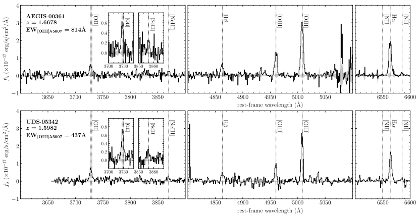
Figure 2: Examples of 1D MMT and Keck spectra of two extreme [O III] emitters at $z=1.3-2.4$. Wavelengths are shifted to the rest-frame. The upper panels show the spectrum of a galaxy with similar equivalent width as the $z\sim 7$ galaxies in the RB16 sample ([O III]$\lambda 5007$ EW $=814$ Å). The lower panels show the spectrum of a galaxy with similar equivalent width as the average value of $z\sim 7$ galaxies in L13 ([O III]$\lambda 5007$ EW $=437$ Å). The $1\sigma$ error spectra are also shown as grey regions. The locations of strong rest-frame optical emission lines are highlighted by black dotted lines. Zoom-in spectra of relatively faint [O II] and [Ne III] emission lines are shown in the left panels. Emission line spectrum of the EW $=814$ Å galaxy shows higher [O III]/[O II] and [Ne III]/[O II] ratios than that of the galaxy with EW $=437$ Å.

The redshift distribution of the 227 galaxies at $z=1.3-2.4$ is shown in Figure 3. The distribution peaks in the $1.55\leq z\leq 1.70$ redshift bin, with 85 of the 227 targets falling in this window. Roughly $29\%$ of the sample ($66/227$) is at $z>2$, and an additional $21\%$ ($48/227$) is at $1.37<z<1.55$. As described above, this latter subset will require optical spectroscopic follow-up for measurement of [O II] and [Ne III]. Our ultimate goal is to provide spectra coverage between [O II] and H$\alpha$ for the majority of extreme line emitters in this sample. In our current sample, we have obtained complete coverage for 53 of the 227 galaxies. The subset with spectral coverage between H$\beta$ and H$\alpha$ is larger (73), with 64 of the 73 sources having robust detections (S/N $>3$) of both H$\alpha$ and H$\beta$. The completeness of our survey and the redshift distribution will change as we acquire more near-infrared and optical spectra in the future.

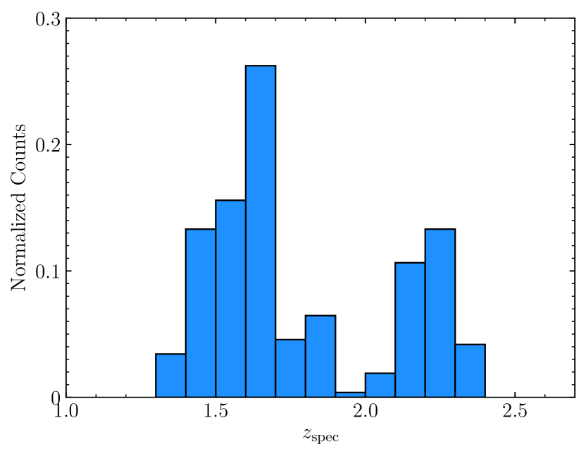
Figure 3: The redshift distribution of the 227 spectroscopically-confirmed extreme emission line galaxies with rest-frame [O III]$\lambda\lambda 4959,5007$ EW $>300$ Å (or identically [O III]$\lambda 5007$ EW $>225$ Å) at $z=1.3-2.4$ in our sample.

Line fluxes are determined from fits to the extracted 1D spectra. We first fit the [O III]$\lambda 5007$ emission line (or H$\alpha$ in the case that [O III] is not available) with a single Gaussian function. The central wavelength from the fit is then used to compute the redshift of the object, which we in turn use to identify the other emission lines. In cases where the lines are well-measured (i.e., S/N $>7$), we derive the flux using a Gaussian fit to the line profile; otherwise we derive the line flux using direct integration. In cases where nearby lines are partially resolved by MMIRS or MOSFIRE, we use multiple Gaussian functions to fit the data. If the flux is measured with S/N $<2$, we consider the line undetected and derive a 2$\sigma$ upper limit. We correct the H$\alpha$ and H$\beta$ fluxes for Balmer absorption using the best-fitting stellar population synthesis models (described in §3). We find that median correction for Balmer lines is less than $10\%$ of the measured emission line fluxes.

The [O III]$\lambda 5007$ emission line fluxes for the extreme line emitters range between $1.1\times$10^-17 erg cm^-2 s^-1 and $6.3\times$10^-16 erg cm^-2 s^-1 with a median of $7.5\times 10^{-17}$ erg cm^-2 s^-1. The range of [O III] fluxes is very similar to those of galaxies in the MOSDEF survey (Kriek et al., 2015); while the equivalent widths in our sample are larger, the continuum magnitudes tend to be fainter than typical MOSDEF sources. The H$\beta$ fluxes of our galaxies are fainter than [O III], with a median of $1.9\times$10^-17 erg cm^-2 s^-1. The emission line fluxes we derive from our ground-based spectra generally agree with the WFC3 grism spectra measurements. We find a median offset of $7\%$ and a scatter of $36\%$, in agreement with the comparison between MOSFIRE spectra and 3D-HST spectra reported by the MOSDEF survey (Kriek et al., 2015).

We estimate the nebular attenuation by comparing the measured Balmer decrement (i.e., the observed H$\alpha$/H$\beta$ intensity ratio) with the value expected by Case B recombination in the case of zero dust reddening, H$\alpha$/H$\beta$ $=2.86$ (assuming electron temperature $T_{e}=10,000$ K; Osterbrock & Ferland 2006). To facilitate comparison with recent near-infrared spectroscopic studies of $z\sim 2$ galaxies (e.g. Reddy et al., 2015; Steidel et al., 2016; Shivaei et al., 2018), we assume the Galactic extinction curve in Cardelli et al. (1989) to compute the dust reddening toward H II regions. We will discuss the extinction values implied by this analysis in §4.1.

To investigate how the average spectral properties vary with optical line equivalent width, we create composite spectra by stacking galaxies in four bins of [O III]$\lambda 5007$ EW: $0-225$ Å, $225-450$ Å, $450-800$ Å, and $800-2500$ Å. We first shift individual spectra to the rest frame using the redshifts measured from [O III]$\lambda 5007$ emission lines. Each spectrum is then interpolated to a common rest-frame wavelength scale of $1$ Å and normalized by the individual H$\alpha$ luminosity (when investigating the average [Ne III]/[O II] ratio in §4.3, we normalize the individual spectrum by its [O III] luminosity since the H$\alpha$ may not be observed in sources used for [Ne III]/[O II] analysis; see also Table 4). To minimize the contribution of sky lines from individual spectra, we stack spectra using inverse-variance weighted luminosities in each wavelength bin (i.e., weighted by $1/\sigma^{2}_{i}$, where $\sigma^{2}_{i}$ is the variation of the $i$th individual spectrum). To check that the resulting composites are not dominated by a few individual spectra, we also create composites using uniform weights and verify that the resulting spectra have similar line measurements as the weighted composite.

The composite spectra for all the four [O III]$\lambda 5007$ EW bins are shown in Figure 4. For these spectra, we have included the subset of our current sample with complete coverage between [O II] and H$\alpha$. There are 7, 26, 13, and 14 galaxies included in the $0-225$ Å, $225-450$ Å, $450-800$ Å, and $800-2500$ Å stacks shown in this figure, respectively. We measure the luminosities of the strong rest-frame optical lines ([O II], [Ne III], H$\beta$, [O III], and H$\alpha$) in each of the four composites. In particular, we are interested in deriving the dependence of the Balmer decrement, and the O32 and Ne3O2 indices on the [O III]$\lambda 5007$ equivalent width. Each line ratio requires slightly different spectral coverage for a robust measurement. For example, the Balmer decrement requires spectra that span between H$\beta$ and H$\alpha$, whereas the dust-corrected O32 measurement requires sources with coverage between [O II] and H$\alpha$, and the Ne3O2 measurement requires sources with coverage between [O II] and [O III]. Accordingly, we can include more objects in the stacks used to investigate the dependence of the Balmer decrement on the [O III]$\lambda 5007$ EW. We will discuss the resulting line ratios in §4. The detailed spectral coverage requirements and the resulting number of objects included in the composite are summarized in Table 4.

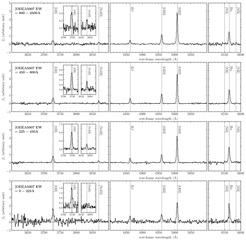
Figure 4: MMT and Keck composite spectra of extreme [O III] emitters at $z=1.3-2.4$, grouped by sources with different [O III]$\lambda 5007$ EWs. The spectra are ranked by [O III]$\lambda 5007$ EW ranges, from the most extreme line emitters ([O III]$\lambda 5007$ EW $=800-2500$ Å) on the top to the objects with similar EWs as the typical galaxies at $z\sim 2$ ([O III]$\lambda 5007$ EW $=0-225$ Å) in the bottom. The $1\sigma$ error spectra are also shown as grey regions. The locations of strong rest-frame optical emission lines are highlighted by black dotted lines. Zoom-in spectra of relatively faint [O II] and [Ne III] emission lines are shown in the left panels. The composite spectra of galaxies with higher [O III]$\lambda 5007$ EWs show higher [O III]/[O II] and [Ne III]/[O II] ratios than those of galaxies with lower EWs.

Sample	Selection criteria	$N$
Extreme [O III] emitters at $z=1.3-2.4$	$z=1.3-2.4$	$227$
H$\alpha$/H$\beta^{1}$ (individual)	[O III]$\lambda 5007$ $>5\sigma$, H$\beta$ and H$\alpha$ $>3\sigma$	$64$
H$\alpha$/H$\beta^{1}$ (composite)	[O III]$\lambda 5007$ $>5\sigma$, spectral coverage between H$\beta$ and H$\alpha$	$73$
[O III]/[O II]2 (individual)	[O III]$\lambda 5007$ $>5\sigma$, [O II]$\lambda\lambda 3727,3729$, H$\beta$ and H$\alpha$ $>3\sigma$	$44$
[O III]/[O II]2 (composite)	[O III]$\lambda 5007$ $>5\sigma$, spectral coverage between [O II]$\lambda\lambda 3727,3729$ and H$\alpha$	$53$
[Ne III]/[O II]3 (individual)	[O III]$\lambda 5007$ $>5\sigma$, [O II]$\lambda\lambda 3727,3729$ and [Ne III]$\lambda 3869$ $>2\sigma$	$26$
[Ne III]/[O II]3 (composite)	[O III]$\lambda 5007$ $>5\sigma$, spectral coverage between [O II]$\lambda\lambda 3727,3729$ and [O III]$\lambda 5007$	$56$

Table 4: Statistics for sub-samples of extreme [O III] emitters ([O III]$\lambda 5007$ EW $>225$ Å) used for line ratio analysis in §4. Spectral coverage requirements and the resulting sub-sample sizes are listed. For each line ratio analysis, individual objects with robust line ratio (Balmer decrement H$\alpha$/H$\beta$, [O III]/[O II], or [Ne III]/[O II]) measurements have more strict requirements than objects used to make composite spectra. For example, the Balmer decrement requires spectra that span between H$\beta$ and H$\alpha$ (73 sources), while measuring robust Balmer decrement in an individual object also requires detecting H$\beta$ and H$\alpha$ with $3\sigma$ significance or higher (64 sources).

Notes.
¹ Sub-sample used for Balmer decrement analysis in §4.1.
² Sub-sample used for [O III]/[O II] ratio analysis in §4.3.
³ Sub-sample used for [Ne III]/[O II] ratio analysis in §4.3.

3 Photoionization Modeling

We fit the broadband fluxes of galaxies in our spectroscopic sample using the Bayesian galaxy SED modeling and interpreting tool BEAGLE (for BayEsian Analysis of GaLaxy sEds, version 0.10.5; Chevallard & Charlot 2016), which incorporates in a consistent way the production of radiation from stars and its transfer through the interstellar and intergalactic media. Broadband photometry is obtained from 3D-HST using the Skelton et al. (2014) catalog, and we utilize multi-wavelength data covering $0.3-2.5\ \mu$m. We also test the impact of adding Spitzer/IRAC constraints for the subset of galaxies that are not strongly confused. For each object, we remove fluxes in filters that lie blueward of Ly$\alpha$ to avoid introducing uncertain contributions from Ly$\alpha$ emission and Ly$\alpha$ forest absorption. We also simultaneously fit the available strong rest-frame optical emission line fluxes ([O II]$\lambda\lambda 3727,3729$, H$\beta$, [O III]$\lambda\lambda 4959,5007$, and H$\alpha$). The version of BEAGLE used in this work adopts the recent photoionization models of star-forming galaxies of Gutkin et al. (2016), which describes the emission from stars and interstellar gas based on the combination of the latest version of Bruzual & Charlot (2003) stellar population synthesis model with the photoionization code CLOUDY (Ferland et al., 2013). The main adjustable parameters of the photoionized gas are the interstellar metallicity, $Z_{\rm{ISM}}$, the typical ionization parameter of a newly ionized H II region, $U_{\rm{S}}$ (which characterizes the ratio of ionizing-photon to gas densities at the edge of the Str$\ddot{\rm{o}}$mgren sphere), and the dust-to-metal (mass) ratio, $\xi_{\rm{d}}$ (which characterizes the depletion of metals on to dust grains). We consider models with C/O abundance ratio equal to the standard value in nearby galaxies (C/O)${}_{\odot}\approx 0.44$. The chosen C/O ratio does not significantly impact the results presented in this paper. We will explore the impact of C/O variations on the derived gas properties in a follow-up paper focused more closely on the photoionization model results. To account for the effect of dust attenuation, we first assume the Calzetti et al. (2000) extinction curve. We also fit galaxies assuming the Small Magellanic Cloud (SMC) extinction curve in Pei (1992). Finally, we adopt the prescription of Inoue et al. (2014) to include the absorption of IGM.

We assume constant star formation history for model galaxies in BEAGLE, and parameterize the maximum age of stars in a model galaxy in the range from 1 Myr to the age of the universe at the given redshift. We fix the redshift of each object to the spectroscopic redshift measured from the MMIRS or MOSFIRE spectra. We adopt a standard Chabrier (2003) initial mass function and assume that all stars in a given galaxy have the same metallicity, in the range $-2.2\leq\log{(Z/Z_{\odot})}\leq 0.25$, where BEAGLE uses the solar metallicity value $Z_{\odot}=0.01524$ from Caffau et al. (2011). The interstellar metallicity is assumed to be the same as the stellar metallicity ($Z_{\rm{ISM}}=Z_{\star}$) for each object. The ionization parameter is allowed to freely vary in the range $-4.0\leq\log{U_{\rm{S}}}\leq-1.0$, and the dust-to-metal mass ratio is allowed to span the range $\xi_{\rm{d}}=0.1-0.5$. We adopt an exponential distribution prior on the V-band dust attenuation optical depths, fixing the fraction of attenuation optical depth arising from dust in the diffuse ISM to $\mu=0.4$ (see Chevallard & Charlot 2016). With the above parameterization, we use the BEAGLE tool to fit the broadband SEDs and available emission line constraints for the $z=1.3-2.4$ galaxies in our sample. Emission line fluxes and broadband fluxes are put on the same absolute scale using the aperture correction procedures described in §2.2. We obtain the output posterior probability distributions of the free parameters described above, and those of other derived physical parameters such as the ionizing photon production efficiency inferred from model ($\xi^{\star}_{\rm{ion}}$). We use the posterior median value as the best-fitting value of each parameter. In Figure 1, we overlay the best-fitting BEAGLE models on the broadband SEDs. It is clear that the models generally do a good job recovering the shape of the continuum and the large flux excesses caused by nebular emission.

The distribution of stellar masses implied by the BEAGLE models is shown in the left panel of Figure 5. Here we include the 64 spectroscopically-confirmed extreme [O III] emitters with spectral coverage between H$\beta$ and H$\alpha$, and with significant detections of H$\beta$ and H$\alpha$ (S/N $>3$). The median stellar mass in this sample is $4.9\times 10^{8}\ M_{\odot}$, well below the typical stellar masses ($\simeq 10^{10}\ M_{\odot}$) found for $z\simeq 2.3$ galaxies in the KBSS and MOSDEF surveys (e.g. Strom et al., 2017; Sanders et al., 2018). We find that galaxies in our sample with the largest [O III] equivalent widths have the lowest stellar masses (see the upper left panel of Figure 6). Among the subset of sources with EW_[OIII]λ5007 in excess of $800$ Å, the median stellar mass is just $4.5\times 10^{7}\ M_{\odot}$. This increases to $4.7\times 10^{8}\ M_{\odot}$ for sources with $450$ Å $<\rm{EW}_{\rm{[OIII]}\lambda 5007}<800$ Å and $1.4\times 10^{9}\ M_{\odot}$ for $225$ Å $<\rm{EW}_{\rm{[OIII]}\lambda 5007}<450$ Å. This variation is to be expected. The near-infrared filters which are sensitive to the stellar mass are heavily contaminated by nebular emission (lines and continuum) in the highest equivalent width systems, implying a smaller contribution from stellar continuum for a given near-infrared magnitude. This effect is further amplified by the dependence of the stellar mass to light ratio on the age of the stellar population. We note that our results do not change significantly when we add Spitzer/IRAC constraints. In particular, we find that the derived stellar masses are always within $0.1$ dex of the values derived without IRAC constraints.

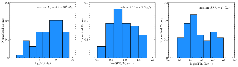
Figure 5: Stellar mass, star formation rate, and specific star formation rate distributions for $z=1.3-2.4$ extreme [O III] emitters ([O III]$\lambda 5007$ EW $>225$ Å) with robust H$\alpha$ and H$\beta$ measurements (S/N $>3$) in our sample (64 of total 73 extreme [O III] emitters with spectral coverage between H$\beta$ and H$\alpha$). Stellar masses, SFRs, and sSFRs are derived from stellar population synthesis modeling using BEAGLE. The median stellar mass is $4.9\times 10^{8}\ M_{\odot}$, the median of SFR is $7.8\ M_{\odot}$yr^-1, and the median of sSFR is $17$ Gyr^-1.

In the middle and right panels of Figure 5, we show the best-fitting model SFR and sSFR of the same 64 line emitters described above. The median of the SFR distribution is $7.8\ M_{\odot}$yr^-1. In contrast to the stellar mass, we do not find strong variations in the SFR with [O III] EW. The median sSFR is $17$ Gyr^-1, well above the average values ($\simeq 2$ Gyr^-1) for galaxies in the KBSS and MOSDEF surveys (e.g. Strom et al., 2017; Sanders et al., 2018). As expected, the sSFR increases with [O III] EW within our sample. The median sSFR ranges from $7.9$ Gyr^-1 ($225$ Å $<\rm{EW}_{\rm{[OIII]}\lambda 5007}<450$ Å) to $21$ Gyr^-1 ($450$ Å $<\rm{EW}_{\rm{[OIII]}\lambda 5007}<800$ Å) to $125$ Gyr^-1 ($800$ Å $<\rm{EW}_{\rm{[OIII]}\lambda 5007}<2500$ Å). The strong variation in sSFR seen in Figure 6 can equivalently be described as a trend in the luminosity weighted age of the stellar population. Under our assumed constant star formation history, the BEAGLE models predict that the median of the maximum stellar age parameter is 130, 50, and 8 Myr for the three [O III]$\lambda 5007$ equivalent width bins described above. These very young values only refer to the burst that is currently dominating the observed SED and do not negate the presence of faint older stars from earlier activity.

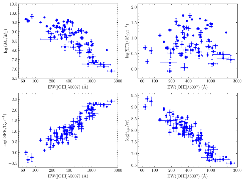
Figure 6: Physical parameters (stellar mass, star formation rate, specific star formation rate, and stellar age) as functions of [O III]$\lambda 5007$ EW for the 77 emission line galaxies with robust H$\alpha$ and H$\beta$ measurements (S/N $>3$) at $z=1.3-2.4$ in our sample (64 extreme [O III] emitters with EW${}_{\rm{[OIII]}\lambda 5007}>225$ Å and 13 additional galaxies with lower EWs). All the parameters are derived from stellar population synthesis modeling using BEAGLE. The upper left, the upper right, the lower left, and the lower right panel shows the stellar mass, the star formation rate, the specific star formation rate, and the stellar age versus [O III]$\lambda 5007$ EW, respectively.

We re-calculate equivalent widths using the newly-obtained near-infrared spectra together with the underlying continuum predicted by BEAGLE. The models provide an improved determination of the continuum, accounting for the emission line contamination in the near-infrared broadband filters. The ground-based spectra provide higher S/N detections of the fainter lines, while also allowing us to separate doublets that are blended in the grism spectra. We calculate the rest-frame equivalent widths of [O II], H$\beta$, [O III]$\lambda 5007$, and H$\alpha$. We will use these measurements when investigating trends with rest-frame optical equivalent widths. In Table 5, we report the [O III]$\lambda 5007$ and H$\alpha$ equivalent widths of the 64 extreme line emitters (EW${}_{\rm{[OIII]}\lambda 5007}>225$ Å) at $z=1.3-2.4$ with robust (S/N $>$3) H$\alpha$ and H$\beta$ detections. We will release the full optical line properties of our sample in a catalog paper after the survey is completed.

Object ID	R.A.	Decl.	$z_{\rm{spec}}$	$m_{\rm{F606W}}$	EW[OIII]λ5007	EWHα
	(hh:mm:ss)	(dd:mm:ss)		(AB)	(Å)	(Å)
AEGIS-29446	14:19:31.989	$+$52:53:22.789	$1.5506$	$26.13\pm 0.10$	$1059\pm 152$	$662\pm 111$
AEGIS-26095	14:19:33.549	$+$52:52:52.797	$1.5625$	$26.19\pm 0.11$	$340\pm 47$	$164\pm 26$
AEGIS-22931	14:19:33.787	$+$52:52:07.560	$2.2953$	$24.05\pm 0.02$	$645\pm 23$	$790\pm 51$
AEGIS-23885	14:19:31.483	$+$52:51:57.961	$1.5721$	$24.64\pm 0.03$	$608\pm 33$	$578\pm 38$
AEGIS-21396	14:19:32.014	$+$52:51:27.694	$2.3206$	$25.35\pm 0.05$	$241\pm 13$	$458\pm 173$
AEGIS-31255	14:19:17.457	$+$52:51:09.896	$1.5970$	$24.42\pm 0.03$	$532\pm 34$	$463\pm 36$
AEGIS-19479	14:19:31.179	$+$52:50:52.304	$1.5969$	$24.79\pm 0.03$	$296\pm 17$	$366\pm 27$
AEGIS-20493	14:19:24.174	$+$52:49:48.020	$1.6725$	$23.73\pm 0.01$	$376\pm 7$	$498\pm 13$
AEGIS-11745	14:19:33.812	$+$52:49:28.451	$1.6069$	$26.15\pm 0.10$	$620\pm 95$	$728\pm 165$
AEGIS-11452	14:19:26.785	$+$52:48:04.364	$1.6720$	$23.33\pm 0.02$	$464\pm 17$	$324\pm 14$
AEGIS-03127	14:20:07.698	$+$52:53:11.858	$2.3089$	$24.51\pm 0.03$	$671\pm 56$	$686\pm 90$
AEGIS-14156	14:19:50.376	$+$52:52:59.100	$1.6738$	$24.86\pm 0.03$	$249\pm 18$	$249\pm 38$
AEGIS-00361	14:20:21.976	$+$52:54:46.588	$1.6678$	$23.78\pm 0.01$	$814\pm 53$	$1028\pm 57$
AEGIS-15032	14:19:26.935	$+$52:49:02.770	$1.6132$	$26.21\pm 0.10$	$1121\pm 210$	$716\pm 170$
AEGIS-04337	14:19:35.878	$+$52:47:54.834	$1.3985$	$26.80\pm 0.16$	$2296\pm 356$	$1876\pm 285$
AEGIS-04711	14:19:34.958	$+$52:47:50.219	$2.1839$	$24.06\pm 0.01$	$1060\pm 25$	$671\pm 33$
AEGIS-16513	14:19:19.204	$+$52:48:00.052	$1.4633$	$24.78\pm 0.03$	$361\pm 24$	$351\pm 28$
AEGIS-24361	14:19:08.525	$+$52:47:59.956	$1.4714$	$25.86\pm 0.07$	$1471\pm 145$	$1192\pm 156$
AEGIS-08869	14:19:20.544	$+$52:46:21.299	$1.5792$	$25.59\pm 0.06$	$909\pm 95$	$1017\pm 88$
AEGIS-15778	14:19:11.210	$+$52:46:23.414	$2.1716$	$25.24\pm 0.04$	$1001\pm 42$	$891\pm 47$
AEGIS-01387	14:19:22.694	$+$52:44:43.040	$2.1700$	$24.77\pm 0.03$	$426\pm 32$	$461\pm 37$
AEGIS-06264	14:19:17.443	$+$52:45:05.370	$2.1879$	$24.72\pm 0.03$	$651\pm 46$	$456\pm 46$
AEGIS-07028	14:19:16.128	$+$52:45:03.763	$2.2925$	$24.91\pm 0.04$	$1023\pm 67$	$783\pm 62$
AEGIS-20217	14:19:02.413	$+$52:45:56.017	$1.6306$	$25.24\pm 0.05$	$341\pm 27$	$601\pm 55$
AEGIS-17118	14:19:03.204	$+$52:45:16.919	$1.6055$	$24.02\pm 0.02$	$332\pm 19$	$376\pm 21$
GOODS-N-38085	12:37:18.165	$+$62:22:29.258	$1.5214$	$24.80\pm 0.02$	$930\pm 79$	$913\pm 80$
GOODS-N-37906	12:37:16.752	$+$62:22:04.152	$1.6847$	$24.65\pm 0.02$	$316\pm 23$	$379\pm 30$
GOODS-N-37876	12:37:12.919	$+$62:21:59.569	$1.6148$	$25.53\pm 0.04$	$283\pm 23$	$357\pm 32$
GOODS-N-37878	12:37:06.160	$+$62:22:00.005	$1.5508$	$25.86\pm 0.05$	$456\pm 46$	$305\pm 32$
GOODS-N-37296	12:37:24.594	$+$62:21:00.900	$1.5136$	$24.47\pm 0.01$	$685\pm 38$	$741\pm 44$
GOODS-N-36886	12:37:31.259	$+$62:20:36.596	$1.6772$	$25.34\pm 0.03$	$1072\pm 144$	$1114\pm 151$
GOODS-N-36583	12:37:33.171	$+$62:20:23.489	$1.5495$	$25.27\pm 0.03$	$480\pm 50$	$699\pm 70$
GOODS-N-36852	12:37:23.247	$+$62:20:34.465	$1.5970$	$25.94\pm 0.06$	$1678\pm 380$	$1209\pm 274$
GOODS-N-36684	12:37:22.580	$+$62:20:26.984	$1.5965$	$25.44\pm 0.04$	$442\pm 44$	$392\pm 40$
GOODS-N-36273	12:37:01.427	$+$62:20:10.543	$2.2422$	$26.05\pm 0.06$	$405\pm 40$	$541\pm 119$
GOODS-N-29675	12:37:07.081	$+$62:17:18.971	$1.6847$	$25.29\pm 0.03$	$561\pm 43$	$938\pm 70$
GOODS-N-35204	12:37:06.813	$+$62:19:35.508	$2.0976$	$23.89\pm 0.01$	$322\pm 12$	$403\pm 29$
UDS-06377	02:17:42.856	$-$05:15:19.134	$1.6642$	$25.31\pm 0.05$	$943\pm 94$	$1169\pm 135$
UDS-12539	02:17:53.733	$-$05:14:03.196	$1.6211$	$24.36\pm 0.02$	$882\pm 33$	$803\pm 31$
UDS-24003	02:17:54.729	$-$05:11:44.020	$1.6205$	$24.55\pm 0.03$	$259\pm 11$	$266\pm 17$
UDS-07447	02:17:18.162	$-$05:15:06.275	$1.5972$	$24.54\pm 0.02$	$666\pm 36$	$529\pm 26$
UDS-13027	02:17:16.355	$-$05:13:56.240	$1.6549$	$25.28\pm 0.04$	$1216\pm 121$	$878\pm 145$
UDS-21873	02:17:17.096	$-$05:12:09.652	$1.6552$	$24.59\pm 0.02$	$271\pm 19$	$387\pm 35$
UDS-15658	02:17:24.262	$-$05:13:25.612	$1.6869$	$24.76\pm 0.04$	$307\pm 23$	$334\pm 34$
UDS-29267	02:17:25.322	$-$05:10:40.397	$1.5190$	$23.77\pm 0.01$	$1893\pm 59$	$1691\pm 73$
UDS-26182	02:17:28.134	$-$05:11:17.272	$1.4867$	$25.45\pm 0.04$	$1120\pm 98$	$1175\pm 137$
UDS-28931	02:17:31.478	$-$05:10:45.926	$1.6000$	$23.33\pm 0.01$	$244\pm 5$	$308\pm 10$
UDS-30015	02:17:36.517	$-$05:10:31.256	$1.6649$	$24.62\pm 0.02$	$917\pm 55$	$607\pm 48$
UDS-19818	02:17:02.612	$-$05:12:34.628	$1.6241$	$25.16\pm 0.04$	$418\pm 35$	$470\pm 47$
UDS-29624	02:17:00.684	$-$05:10:34.903	$1.6632$	$26.26\pm 0.11$	$881\pm 195$	$779\pm 208$
UDS-36954	02:17:14.900	$-$05:09:06.174	$1.6578$	$25.41\pm 0.04$	$238\pm 20$	$347\pm 68$
UDS-14019	02:17:28.554	$-$05:13:44.857	$1.4612$	$23.80\pm 0.01$	$490\pm 15$	$614\pm 17$
UDS-05122	02:17:22.253	$-$05:15:33.613	$1.4628$	$24.67\pm 0.03$	$307\pm 16$	$291\pm 14$
UDS-05342	02:17:09.216	$-$05:15:31.990	$1.5981$	$23.58\pm 0.01$	$437\pm 12$	$363\pm 8$
UDS-11693	02:17:03.893	$-$05:14:13.664	$2.1854$	$24.52\pm 0.02$	$596\pm 33$	$592\pm 73$
UDS-15128	02:17:38.209	$-$05:13:32.092	$2.3113$	$24.25\pm 0.02$	$371\pm 16$	$276\pm 97$
UDS-12435	02:17:38.609	$-$05:14:05.366	$1.6112$	$24.06\pm 0.01$	$247\pm 9$	$173\pm 6$
UDS-11387	02:17:39.228	$-$05:14:17.689	$1.4048$	$24.64\pm 0.02$	$602\pm 40$	$469\pm 34$
UDS-17713	02:17:42.450	$-$05:13:02.615	$2.2484$	$24.09\pm 0.02$	$328\pm 16$	$249\pm 50$

Table 5: Summary of the 64 extreme [O III] emitters (EW${}_{\rm{[OIII]}\lambda 5007}>225$ Å) with robust Balmer line detections (S/N $>3$) at $z=1.3-2.4$. Column (1): galaxy ID in 3D-HST v4 catalogs; Column (2): right ascension of the galaxy; Column (3): declination of the galaxy; Column (4): redshift measured from MMT or Keck spectra; Column (5): HST F606W magnitude (in AB magnitude); Column (7): rest-frame [O III]$\lambda 5007$ equivalent width; Column (8): rest-frame H$\alpha$ equivalent width.

Object ID	R.A.	Decl.	$z_{\rm{spec}}$	$m_{\rm{F606W}}$	EW[OIII]λ5007	EWHα
	(hh:mm:ss)	(dd:mm:ss)		(AB)	(Å)	(Å)
UDS-28064	02:17:47.396	$-$05:10:56.197	$1.4600$	$24.54\pm 0.03$	$360\pm 27$	$203\pm 16$
UDS-24183	02:17:47.395	$-$05:11:41.453	$2.2448$	$24.97\pm 0.04$	$821\pm 59$	$756\pm 132$
UDS-22532	02:17:52.799	$-$05:12:03.013	$1.4207$	$24.62\pm 0.03$	$387\pm 12$	$197\pm 7$
UDS-17891	02:17:45.950	$-$05:12:57.416	$1.6714$	$25.99\pm 0.07$	$1673\pm 552$	$1300\pm 435$
UDS-12980	02:17:55.822	$-$05:13:56.748	$1.4102$	$25.50\pm 0.05$	$625\pm 53$	$725\pm 96$

Table 5: Continued.

The BEAGLE models allow us to characterize the production efficiency of hydrogen ionizing photons in the EELGs. There are various definitions of this quantity in the literature. We follow the nomenclature used in our earlier work (Chevallard et al., 2018) which we briefly review below. First, we define $\xi^{\star}_{\rm{ion}}$ as the hydrogen ionizing photon production rate ($N(\rm{H}^{0})$) per unit UV stellar continuum luminosity ($L^{\star}_{\rm{UV}}$). The quantity $L^{\star}_{\rm{UV}}$ is the luminosity produced by the stellar population prior to its transmission through the gas and dust in the galaxy, and as such it does not include nebular continuum emission or absorption from the ISM. As is commonplace, we evaluate the UV luminosity at a rest-frame wavelength of $1500$ Å. BEAGLE includes a determination of $\xi^{\star}_{\rm{ion}}$ in its output parameter file for each source. Secondly, we define $\xi_{\rm{ion}}$, as the hydrogen ionizing photon production rate per unit observed UV luminosity ($L_{\rm{UV}}$), again evaluated at $1500$ Å. $L_{\rm{UV}}$ includes emission from the stellar population and nebular continuum and is not corrected for the attenuation provided by the ISM. Finally we define $\xi^{\rm{HII}}_{\rm{ion}}$ as the hydrogen ionizing photon production rate per unit $L^{\rm{HII}}_{\rm{UV}}$, the observed UV luminosity at $1500$ Å (including nebular and stellar continuum) corrected for dust attenuation from the diffuse ISM. This is the most commonly used definition of the hydrogen ionizing production efficiency in the literature, and we will focus primarily on this quantity in the following section.

In deriving $\xi^{\rm{HII}}_{\rm{ion}}$, we follow a similar procedure adopted in several recent studies (Matthee et al., 2017; Shivaei et al., 2018). We compute the H$\alpha$ luminosity from our spectra and apply a correction for dust attenuation using the measured Balmer decrement (see §2.5). We then calculate the ionizing photon production rate from the H$\alpha$ luminosity (Osterbrock & Ferland, 2006):

$$L(\textrm{H}\alpha)\ [\textrm{erg s}^{-1}]=1.36\times 10^{-12}\ N(\textrm{H}^{0})\ [\textrm{s}^{-1}].$$ (1)

This assumes radiation-bounded nebula, with negligible escape of ionizing radiation. The dust correction through the Balmer decrement traces dust only outside the H II regions, and does not account for the absorption of ionizing photons before they ionize hydrogen (Petrosian et al., 1972; Mathis, 1986; Charlot & Fall, 2000). Thus, the $N(\rm{H}^{0})$ computed in Eq. (1) is somewhat lower than the true production rate of ionizing photons emitted by stars. However, in §4.1 we demonstrate that the extreme [O III] emitters in our sample have very little dust, indicating that the effect of absorption of ionizing photons inside the H II regions should be very small. We infer the observed UV continuum luminosity from the best-fitting BEAGLE model using a flat $100$ Å filter centered at $1500$ Å. We then apply a dust correction using the reddening inferred from BEAGLE assuming first a Calzetti and then a SMC extinction law. Finally, the ionizing photon production efficiency $\xi^{\rm{HII}}_{\rm{ion}}$ is computed as follows:

$$\xi^{\textrm{HII}}_{\textrm{ion}}\ [\textrm{erg}^{-1}\ \textrm{Hz}]=\frac{N(\textrm{H}^{0})\ [\textrm{s}^{-1}]}{L^{\textrm{HII}}_{\textrm{UV}}\ [\textrm{erg s}^{-1}\ \textrm{Hz}^{-1}]}.$$ (2)

In the following section, we will investigate how the ionizing production efficiency varies with the nebular line equivalent widths. Here we attempt to build some basic physical intuition about this relationship. Since the [O III] and H$\alpha$ EW are directly linked to the luminosity-weighted age of the stellar population, the variation of $\xi^{\star}_{\rm{ion}}$ will mirror the time evolution of $N(\rm{H}^{0})$ and $L^{\star}_{\rm{UV}}$, the former powered by O stars and the latter by O to early B stars. For the very young stellar populations probed by the most extreme line emitting galaxies in our sample (EW${}_{\rm{H}\alpha}>1000$ Å), the ratio of O to B stars will be maximized, resulting in very efficient ionizing photon production. Among more moderate line emitters (EW${}_{\rm{H}\alpha}=400-600$ Å), a larger population of B stars will have emerged, boosting $L_{\rm{UV}}$ relative to $N(\rm{H}^{0})$. The ionizing production efficiency will thus be reduced for these systems. Finally, at yet lower equivalent width (EW${}_{\rm{H}\alpha}=50-200$ Å), the O and B star populations will be closer to equilibrium, with the number of newly-formed stars nearly balanced by those exiting the main sequence. As a result, both $N(\rm{H}^{0})$ and $L_{\rm{UV}}$ will not vary significantly with age, and the production efficiency of ionizing photons should thus begin to plateau to a near-constant value for galaxies with EW${}_{\rm{H}\alpha}<200$ Å. While this basic physical picture guides our expectations, the precise dependence of $\xi^{\star}_{\rm{ion}}$ on the [O III] and H$\alpha$ equivalent width depends on unknown physics (i.e., binary stars, rotation) governing the formation of hot stars. Empirical constraints on $\xi^{\star}_{\rm{ion}}$ are thus critical for assessing the ionizing output of early galaxies.

4 rest-frame optical Spectroscopic Properties of Extreme [O III] Emitters at $z=1.3-2.4$

We now investigate what the rest-frame optical spectra reveal about the radiation field and gas conditions of galaxies with large equivalent width rest-frame optical nebular line emission. We will focus primarily on empirical trends that can be extracted from line ratios, leaving a more detailed analysis of the photoionization models to a later paper. In §4.1, we use measurements of the Balmer decrements to constrain the nebular attenuation. We then characterize the radiation field and gas conditions through measurement of the ionizing photon production efficiency (§4.2) and standard ionization-sensitive emission line ratios (§4.3).

4.1 Balmer Decrement Measurements

The physical interpretation of our spectra requires robust determination of the nebular attenuation between [O II] and H$\alpha$. As introduced in §2.5, this is most commonly done through comparison of the Balmer decrement, $I(\rm{H}\alpha)/I(\rm{H}\beta)$, to the ratio expected in absence of dust. As noted in §3, the Balmer decrement corrects for dust outside the H II regions but does not account for the possible absorption of LyC photons by dust before they ionize hydrogen. The first statistical measurements of the Balmer decrement distribution at high redshift have begun to emerge from the KBSS and MOSDEF surveys (e.g. Reddy et al., 2015; Steidel et al., 2016). These investigations provide an important baseline for comparison to the extreme emission line galaxies in our sample, so we briefly review the results below. To enable comparison with investigations of nebular attenuation in the KBSS and MOSDEF galaxies, here we adopt a Cardelli et al. (1989) extinction curve.

The average nebular properties of the KBSS survey are well described by the KBSS-LM1 composite spectrum, a weighted average of galaxies at $z\simeq 2.11-2.57$ with median stellar mass of $6\times$10${}^{9}\ M_{\odot}$ and specific star formation rate of $3.5$ Gyr^-1 (Steidel et al., 2016) The Balmer decrement derived from the composite is $I(\rm{H}\alpha)/I(\rm{H}\beta)=3.61\pm 0.07$ (Steidel et al., 2016), similar to that found in individual KBSS galaxies (Strom et al., 2017). For the MOSDEF survey, the average Balmer decrement measured from a composite of 213 galaxies with significant H$\beta$ detections is $I(\rm{H}\alpha)/I(\rm{H}\beta)=4.1$ (Reddy et al., 2015). For a Cardelli et al. (1989) Galactic extinction curve and an intrinsic Balmer decrement, $I(\rm{H}\alpha)/I(\rm{H}\beta)=2.86$, the KBSS and MOSDEF composites imply typical color excesses of $E(B-V)_{\rm{gas}}=0.22$ and $0.36$, respectively. We note that Steidel et al. (2016) adopt a slightly larger intrinsic Balmer decrement, $I(\rm{H}\alpha)/I(\rm{H}\beta)=2.89$, that is consistent with their photoionization model fits. As a result, they report a slightly different color excess, $E(B-V)_{\rm{gas}}=0.21$, for the KBSS-LM1 composite.

In our current sample, we can measure Balmer decrements in 64 extreme emission line galaxies (EW${}_{\rm{[OIII]}\lambda 5007}>225$ Å) with significant detections (S/N $>3$) of H$\alpha$ and H$\beta$ (Table 4). The measurements suggest that extreme line emitters suffer less nebular attenuation than most galaxies in the KBSS and MOSDEF surveys. In Figure 7, we show the distribution of Balmer decrements for EELGs in our sample with EW${}_{\rm{[OIII]}\lambda 5007}>450$ Å. This threshold is chosen to correspond roughly to the average [O III]+H$\beta$ equivalent width at $z\simeq 7-8$ (L13), assuming an [O III]/H$\beta$ ratio that is characteristic of EELGs (see §2.1). The average Balmer decrement in this histogram is $I(\rm{H}\alpha)/I(\rm{H}\beta)=3.09$, implying a color excess of just $E(B-V)_{\rm{gas}}=0.08$ for the Cardelli et al. (1989) extinction curve. For reference we also measure $\beta$, the UV continuum slope, for this same subset of galaxies. We compute the UV slope from broadband fluxes by fitting a power-law ($f_{\lambda}\propto\lambda^{\beta}$) at rest-frame wavelengths $1250-2600$ Å (the same wavelength range used in Calzetti et al. 1994; filters covering Ly$\alpha$ emission line are not included). The resulting UV slopes are very blue, with a median of $\beta=-2.04$ for galaxies with EW${}_{\rm{[OIII]}\lambda 5007}>450$ Å, implying that the stars are also minimally reddened by dust.

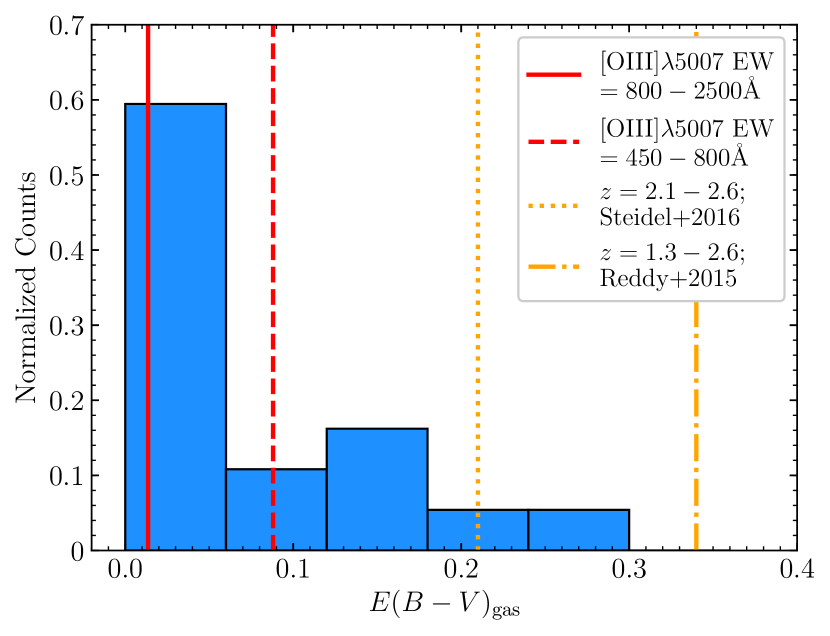
Figure 7: Probability distribution of nebular dust reddening for extreme [O III] emitters with EW${}_{\rm{[OIII]}\lambda 5007}>450$ Å at $z=1.3-2.4$. The extinction $E(B-V)_{\rm{gas}}$ is inferred from Balmer decrement, assuming the Cardelli et al. (1989) extinction curve and intrinsic H$\alpha$/H$\beta$ intensity ratio $=2.86$. The extinction values inferred from composite spectra of extreme [O III] emitters with EW${}_{\rm{[OIII]}\lambda 5007}=800-2500$ Å and EW${}_{\rm{[OIII]}\lambda 5007}=450-800$ Å are plotted by red solid and dashed lines. For comparison, we also show the extinction values inferred from more massive, older systems at $z\sim 2$ from KBSS (Steidel et al., 2016) as the orange dotted line and MOSDEF survey (Reddy et al., 2015) as the orange dashed-dotted line.

The level of nebular attenuation varies with the [O III] EW, with the most extreme line emitters having the least dust. In our sample, the median Balmer decrement for the 16 galaxies with EW${}_{\rm{[OIII]}\lambda 5007}=450-800$ Å is $I(\rm{H}\alpha)/I(\rm{H}\beta)=3.12$. When we consider the 21 more extreme line emitters with EW${}_{\rm{[OIII]}\lambda 5007}=800-2500$ Å, we find a Balmer decrement of just $I(\rm{H}\alpha)/I(\rm{H}\beta)=2.95$. This implies color excesses of $E(B-V)_{\rm{gas}}=0.09$ and $0.03$ for the two respective EW bins. The composite spectra reveal a similar picture. The measured Balmer decrement in the stacks decreases from $I(\rm{H}\alpha)/I(\rm{H}\beta)=3.12\pm 0.04$ (EW${}_{\rm{[OIII]}\lambda 5007}=450-800$ Å) to $I(\rm{H}\alpha)/I(\rm{H}\beta)=2.90\pm 0.05$ (EW${}_{\rm{[OIII]}\lambda 5007}=800-2500$ Å). This indicates that among the most extreme line emitters, the Balmer decrements are very close to the intrinsic case B recombination value (for $T_{e}=10^{4}$ K gas), suggesting that the emission lines in these galaxies face little to no attenuation from dust.

The results described above clearly demonstrate that the EELG population has a different distribution of Balmer decrements than the typical KBSS and MOSDEF galaxies. This result is not surprising given trends between the Balmer decrement and galaxy properties found previously (Reddy et al., 2015), likely reflecting both the low stellar mass (and hence moderately low metallicities) and large specific star formation rates (and hence young stellar populations) of the galaxies in our sample (Figure 6). Importantly this implies that very small adjustments are required to correct the observed fluxes for reddening.

An important consequence is that uncertainties in the high redshift attenuation law should not significantly affect our interpretation of the nebular line spectra of EELGs. Among more massive star forming galaxies at $z\simeq 2$, this is not always the case. Shivaei et al. (2018) demonstrated that the $\xi^{\rm{HII}}_{\rm{ion}}$ inferred assuming a Calzetti attenuation law is systematically 0.3 dex lower than that derived for an SMC attenuation law, making it difficult to robustly determine $\xi^{\rm{HII}}_{\rm{ion}}$. While our measurements of $\xi^{\rm{HII}}_{\rm{ion}}$ also depend on the assumed dust law, the variation is typically only 0.1 dex when considering the SMC and Calzetti attenuation laws. For the most extreme line emitting sources (EW${}_{\rm{[OIII]}\lambda 5007}>800$ Å), the dust content is low enough that the average offset in $\xi^{\rm{HII}}_{\rm{ion}}$ is just 0.05 dex.

4.2 The Ionizing Photon Production Efficiency

As a first step in our investigation of the radiation field of extreme emission line galaxies, we characterize the production efficiency of hydrogen ionizing photons in our spectroscopic sample. Recent efforts have quantified $\xi^{\rm{HII}}_{\rm{ion}}$ in more massive star forming galaxies at $z\simeq 2$ (e.g Matthee et al., 2017; Shivaei et al., 2018), revealing typical values of $\log{[\xi^{\rm{HII}}_{\rm{ion}}\ (\rm{erg}^{-1}\ \rm{Hz})]}=25.06$ for a Calzetti UV attenuation law (Shivaei et al., 2018). These systems tend to have [O III]$\lambda 5007$ equivalent widths of $115$ Å (see §2.1), well below those considered in this paper, as expected from older stellar populations. It has been shown that $\xi^{\star}_{\rm{ion}}$ scales with the [O III] equivalent width among local star forming galaxies (Chevallard et al., 2018), suggesting that the higher equivalent width systems which become common in the reionization era may be more efficient ionizing agents. Here we seek to investigate whether a similar relationship between the ionizing production efficiency and optical lines holds at $z\simeq 1-2$. In the following, we will first describe the distribution of $\xi^{\rm{HII}}_{\rm{ion}}$ values, using the dust corrections discussed in §3. Then we will compare our measurements of $\xi^{\star}_{\rm{ion}}$ to the relation found locally, investigating whether there is any evidence for strong redshift evolution in $\xi^{\star}_{\rm{ion}}$ values at fixed [O III] EW.

Our current sample contains 64 large equivalent width [O III] emitters (EW${}_{\rm{[OIII]}\lambda 5007}>225$ Å) with the spectroscopic measurements of H$\alpha$ and H$\beta$ necessary to infer $\xi^{\rm{HII}}_{\rm{ion}}$. In Figure 8, we show the implied $\xi^{\rm{HII}}_{\rm{ion}}$ values as a function of the [O III]$\lambda 5007$ and H$\alpha$ equivalent widths. It is immediately clear that $\xi^{\rm{HII}}_{\rm{ion}}$ scales with both optical lines at EW${}_{\rm{[OIII]}\lambda 5007}>225$ Å. We first consider galaxies with EW${}_{\rm{[OIII]}\lambda 5007}\simeq 450$ Å. For the [O III]/H$\beta$ line ratios exhibited by extreme emission line galaxies (see §2.1), this [O III]$\lambda 5007$ EW is comparable to that implied by IRAC flux excesses in composite SEDs of $z\simeq 7-8$ galaxies (L13). To estimate the typical ionizing efficiency for galaxies with this [O III] EW, we group those systems in our sample with EW${}_{\rm{[OIII]}\lambda 5007}=300-600$ Å. Assuming a Calzetti attenuation law for the UV, the median ionizing production efficiency of this sub-sample is $\log{[\xi^{\rm{HII}}_{\rm{ion}}\ (\rm{erg}^{-1}\ \rm{Hz})]}=25.22$, $\sim 1.5\times$ greater than found in more typical galaxies at $z\simeq 2$ (Shivaei et al., 2018). For an SMC extinction law for the UV, the ionizing production efficiency is $\log{[\xi^{\rm{HII}}_{\rm{ion}}\ (\rm{erg}^{-1}\ \rm{Hz})]}=25.32$, slightly larger than what we found above for the Calzetti law. This suggests that galaxies which are common at $z\gtrsim 6$ should make a greater contribution to reionization than was originally thought, as has been noted by several recent investigations of IRAC excesses and UV metal lines at $z\gtrsim 5$ (Rasappu et al., 2016; Stark et al., 2015b, 2017).

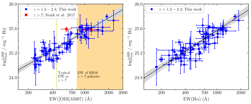
Figure 8: Left Panel: Relation between the ionizing photon production efficiency $\xi^{\rm{HII}}_{\rm{ion}}$ and [O III]$\lambda 5007$ EW for the $z=1.3-2.4$ galaxies in our sample (blue circles). The $\xi^{\rm{HII}}_{\rm{ion}}$ is computed based on the spectroscopic measurements of H$\alpha$ and H$\beta$. A linear relation is fitted between $\xi^{\rm{HII}}_{\rm{ion}}$ and $\log{\rm{EW}_{\rm{[OIII]}\lambda 5007}}$ (black dashed line, with grey area shows the 95 percent credible region). The average EW of $z\simeq 7-8$ galaxies (EW${}_{\rm{[OIII]}\lambda 5007}\simeq 450$ Å; L13) is highlighted by yellow dashed line. The orange area shows EWs of $z>7$ galaxies in RB16, and red squares show the individual sources in RB16, in which the $\xi^{\rm{HII}}_{\rm{ion}}$ are inferred from photoionization models (Stark et al., 2017). Right Panel: Relation between $\xi^{\rm{HII}}_{\rm{ion}}$ and H$\alpha$ EW for the $z\sim 2$ galaxies in our sample (blue circles). A linear relation is fitted between $\xi^{\rm{HII}}_{\rm{ion}}$ and $\log{\rm{EW}_{\rm{H}\alpha}}$ (black dashed line, with grey area shows the 95 percent credible region).

Attention is now focused on galaxies at $z\gtrsim 7$ with even larger [O III] equivalent widths (EW${}_{\rm{[OIII]}\lambda 5007}=800-2500$ Å). While such sources may not be the norm at $z\gtrsim 7$, they are readily detectable in the CANDELS fields (e.g. Roberts-Borsani et al., 2016) and appear to have an enhanced Ly$\alpha$ visibility at redshifts where the IGM is thought to be significantly neutral (e.g. Oesch et al., 2015; Zitrin et al., 2015; Stark et al., 2017). One possible explanation is that these systems are situated in the largest ionized bubbles, thereby allowing enhanced transmission of their Ly$\alpha$ radiation. Alternatively, in addition to sitting in ionized bubbles, the galaxies may be producing more Ly$\alpha$ than other galaxies of similar far-UV luminosities. This would follow if the production efficiency of Lyman-alpha is larger in systems with the most prominent [O III] emission.

Our results provide some insight into the situation. Since Ly$\alpha$ is produced by reprocessed hydrogen ionizing photons, the Ly$\alpha$ production efficiency ($L_{\rm{Ly}\alpha}/L^{\rm{HII}}_{\rm{UV}}$) should be directly correlated with $\xi^{\rm{HII}}_{\rm{ion}}$. Sources that are efficient at producing ionizing radiation should also be efficient in powering Ly$\alpha$ emission. In Figure 8, we see that the production efficiency of ionizing radiation steadily increases between EW${}_{\rm{[OIII]}\lambda 5007}=450$ Å and $2500$ Å. Among those sources with EW${}_{\rm{[OIII]}\lambda 5007}>800$ Å, the production efficiency has a median of $\log{[\xi^{\rm{HII}}_{\rm{ion}}\ (\rm{erg}^{-1}\ \rm{Hz})]}=25.58$ (Calzetti) and $25.62$ (SMC). This value is very similar to estimates of $\xi^{\rm{HII}}_{\rm{ion}}$ in the RB16 sample of $z\gtrsim 7$ galaxies with similarly strong [O III] (see red squares in Figure 8). Our results suggest that galaxies with [O III] EWs similar to the RB16 galaxies may produce two times more ionizing photons than typical reionization-era sources (the latter of which have EW${}_{\rm{[OIII]}\lambda 5007}\simeq 450$ Å) with similar non-ionizing UV luminosities. The larger-than-average Ly$\alpha$ equivalent widths that we are now seeing in the RB16 population should thus partially reflect an enhanced production of ionizing radiation. In §5.2, we will explore in more detail whether variations in internal galaxy properties can explain the anomalous visibility of Ly$\alpha$ that is now being found in strong [O III] emitters at $z\gtrsim 7$.

The relationship between the production efficiency of ionizing photons and the [O III]$\lambda 5007$ EW shown in Figure 8 can be described by a simple scaling law. We fit a linear relation between the two quantities for those galaxies in our sample with $225$ Å $<\rm{EW}_{\rm{[OIII]}\lambda 5007}<2500$ Å. The best-fit relation for the Calzetti UV attenuation law is

$$\log{\xi^{\textrm{HII}}_{\textrm{ion}}} = (0.76\pm 0.05)\times\log{(\textrm{EW [O {\scriptsize III}]}\lambda 5007)}+$$ (3)

$$(23.27\pm 0.15).$$

For an SMC attenuation law, we find a very similar relationship:

$$\log{\xi^{\textrm{HII}}_{\textrm{ion}}} = (0.73\pm 0.08)\times\log{(\textrm{EW [O {\scriptsize III}]}\lambda 5007)}+$$ (4)

$$(23.45\pm 0.23).$$

The derived fitting function is overlaid on the data in Figure 8. We emphasize that the scaling laws is only valid for the large equivalent widths stated above. Indeed, as we motivated at the end of §3, we expect $\xi^{\rm{HII}}_{\rm{ion}}$ may deviate from the relationship at lower equivalent widths. But for sources with EW${}_{\rm{[OIII]}\lambda 5007}>225$ Å, these fitting functions can be used to predict the distribution of $\xi^{\rm{HII}}_{\rm{ion}}$ given an observed distribution of [O III] equivalent widths. As suggested in Chevallard et al. (2018), and provided that this relationship does not evolve strongly with redshift (as we will show below for $0<z<2$), this can be used in conjunction with IRAC flux excesses to estimate the production efficiency of ionizing photons in the reionization era.

We can also derive a relationship between H$\alpha$ and $\xi^{\rm{HII}}_{\rm{ion}}$ using the results in Figure 8. Because the H$\alpha$ strength is less sensitive to the gas physical conditions than [O III], we expect it to have a more universal relationship with the ionizing production efficiency. Applying a similar fitting procedure and assuming a Calzetti attenuation law for the UV, we derive the following relationship:

$$\log{\xi^{\textrm{HII}}_{\textrm{ion}}} = (0.85\pm 0.06)\times\log{(\textrm{EW H}\alpha)}+$$ (5)

$$(23.03\pm 0.15).$$

For the SMC law, we again find a very similar relationship:

$$\log{\xi^{\textrm{HII}}_{\textrm{ion}}} = (0.87\pm 0.07)\times\log{(\textrm{EW H}\alpha)}+$$ (6)

$$(23.06\pm 0.19).$$

To assess the magnitude of the redshift evolution in the relationship between the production efficiency and the rest-frame optical line equivalent widths, we compare our results to those derived for local galaxies in Chevallard et al. (2018). The local galaxy relation is derived using $\xi^{\star}_{\rm{ion}}$, the ratio of the intrinsic production rate of ionizing photons to the stellar continuum luminosity in the non-ionizing far-UV, with both quantities derived from BEAGLE model fits to the data (see definitions in §3). In cases where the nebular continuum contributes significantly to the observed UV luminosity, we expect $\xi^{\star}_{\rm{ion}}$ to deviate from $\xi^{\rm{HII}}_{\rm{ion}}$, providing a more realistic description of the efficiency of a stellar population at producing ionizing radiation. We find that $\xi^{\star}_{\rm{ion}}$ is indeed systematically larger than $\xi^{\rm{HII}}_{\rm{ion}}$ in our sample, but the differences are relatively small. Among galaxies with [O III]$\lambda 5007$ equivalent widths between $450$ and $800$ Å ($800$ and $2500$ Å), the difference is 0.04 (0.08) dex. This suggests that the relations between $\xi^{\rm{HII}}_{\rm{ion}}$ and optical line equivalent widths that we derived above should closely approximate those inferred using $\xi^{\star}_{\rm{ion}}$. Nevertheless for the sake of consistency, we consider trends with $\xi^{\star}_{\rm{ion}}$ when comparing the production efficiencies derived at $z=1.3-2.4$ with those found locally.

In Figure 9, we show the dependence of $\xi^{\star}_{\rm{ion}}$ on the H$\beta$ and [O III] EW for our high redshift sample (blue circles) and the nearby galaxies (green squares) investigated in Chevallard et al. (2018). The local sample is comprised of ten systems with deep UV and optical spectra (Senchyna et al., 2017), each selected to have extreme radiation fields based on the presence of He II emission. The relationship between $\xi^{\star}_{\rm{ion}}$ and H$\beta$ EW appears largely similar in the two redshift samples. We can quantify this by comparing the linear fit to the $\log{\xi^{\star}_{\rm{ion}}}-\log{\rm{EW}_{\rm{H}\beta}}$ relationship in the range EW${}_{\rm{H}\beta}=80-400$ Å. The best-fit slope and intercept for the $z\simeq 0$ sample ($1.23\pm 0.25$ and $22.89\pm 0.56$) are both consistent (within $1\sigma$) with those derived for the $z\simeq 2$ galaxies ($1.09\pm 0.07$ and $23.23\pm 0.16$). Given the dependence of [O III] on ionized gas conditions (i.e., metallicity, ionization parameter), we expect the relationship between [O III] EW and $\xi^{\star}_{\rm{ion}}$ may potentially show more variation with redshift. However, the current data reveal little evidence to this effect. The best fit intercept and slope at $z\simeq 0$ ($1.14\pm 0.16$ and $22.28\pm 0.44$) remain broadly similar (within $2\sigma$) to those derived at $z\simeq 2$ ($0.88\pm 0.06$ and $22.98\pm 0.16$). While larger samples may eventually reveal some mild differences, our results suggest that the redshift evolution in the relationship between $\xi^{\star}_{\rm{ion}}$ and the H$\beta$ and [O III] EW is not likely to be strong.

Figure 9: BEAGLE model-derived $\xi^{\star}_{\rm{ion}}$ as a function of H$\beta$ EW (left panel) and [O III]$\lambda 5007$ EW (right panel) at $z=1.3-2.4$ (blue circles; this work) and $z\sim 0$ (green squares; Chevallard et al. 2018). The $\xi^{\star}_{\rm{ion}}$ is computed based on the intrinsic UV stellar luminosity (assuming a SMC extinction curve in order to be consistent with Chevallard et al. 2018), and only objects with similar EWs in the two samples (H$\beta$ EW $=80-400$ Å in the left panel; [O III]$\lambda 5007$ EW $=400-2500$ Å in the right panel) are shown.

4.3 The Physical Conditions of the Nebular Gas

The results of §4.2 show that extreme emission line galaxies are considerably more efficient at producing ionizing radiation than the more massive star-forming galaxies which are typical at $z\sim 2$. The intense radiation field of these system may impact the ionization state of the ISM, potentially aiding the escape of Ly$\alpha$ and LyC radiation. In this subsection, we investigate the ISM of extreme emission line galaxies by quantifying the dependence of [O III]/[O II] (O32) and [Ne III]/[O II] (Ne3O2), two ionization-sensitive emission line ratios, on the [O III] and H$\alpha$ EW.

The O32 index is one of the most commonly used probes of nebular gas ionization state and is often employed as an empirical proxy for the ionization parameter (the ratio of the number density of incident hydrogen-ionizing photons to the number density of hydrogen atoms in the H II region; Penston et al. 1990). The average O32 ratios of the massive star forming galaxies in the KBSS (O32 $=2.0$; Steidel et al. 2016) and MOSDEF (median O32 $=1.3$; Sanders et al. 2016) surveys are $\sim 4-7\times$ higher than those of $z\sim 0$ galaxies with similar stellar masses (median O32 $=0.3$; Abazajian et al. 2009; Sanders et al. 2016). While the origin of the higher ionization parameters remains a matter of some debate, it has been argued to reflect a shift toward lower metallicities at fixed mass in high redshift galaxies (Sanders et al., 2016).

The extreme emission line galaxies targeted in our survey have lower stellar masses and higher specific star formation rates than most galaxies from the KBSS and MOSDEF surveys (see §3). Both factors could lead to different ionization conditions. Our current sample contains O32 measurements with dust corrections via the Balmer decrement for 44 galaxies (Table 4) with large equivalent width [O III] emission (EW${}_{\rm{[OIII]}\lambda 5007}>225$ Å). In the top panel of Figure 10, we show the dependence of O32 on the [O III]$\lambda 5007$ EW for individual galaxies (blue circles) and for our composite spectra (red squares). The results clearly demonstrate that O32 increases with the [O III]$\lambda 5007$ EW, indicating more extreme ionizing conditions in the high EW galaxies. The composite spectra reveal [O III]/[O II] ratios of O32 $=1.4\pm 0.2$, $3.6\pm 0.2$, $4.8\pm 0.3$, and $9.1\pm 0.5$ for stacks including galaxies with EW${}_{\rm{[OIII]}\lambda 5007}=0-225$ Å, $225-450$ Å, $450-800$ Å, and $800-2500$ Å, respectively.

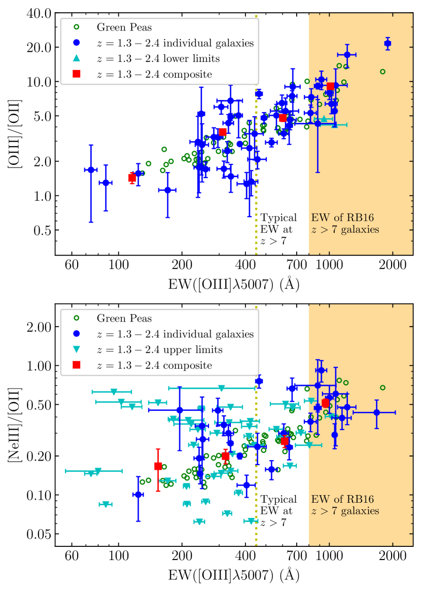
Figure 10: Relation between [O III]$\lambda 5007$ EW and ionization-sensitive line ratios ([O III]/[O II], upper panel; [Ne III]/[O II], lower panel) of the $z=1.3-2.4$ galaxies in our sample (blue circles). Line ratios of objects without robust [O II] (cyan triangles in the upper panel) or [Ne III] detections (cyan upside-down triangles in the lower panel) are shown as $2\sigma$ lower or upper limits. The average line ratios derived from composite spectra of galaxies with different EWs are shown by red squares. The average EW of $z\simeq 7-8$ galaxies (L13) is highlighted by yellow dashed line, and the orange area shows EWs of $z>7$ galaxies in the RB16 sample. For comparison, [O III]$\lambda 5007$ EWs and line ratios of Green Peas (Cardamone et al., 2009; Hawley, 2012) are shown by green open circles.

We see a comparable O32 trend in the individual galaxy measurements. For galaxies with EW${}_{\rm{[OIII]}\lambda 5007}=300-600$ Å (similar to the average EW expected in the reionization era), we find a median [O III]/[O II] ratio of O32 $=3.5$. Among the galaxies in our sample with [O III] equivalent widths comparable to the RB16 $z\gtrsim 7$ Ly$\alpha$ emitters (EW${}_{\rm{[OIII]}\lambda 5007}=800-2500$ Å), we find evidence for even more extreme ISM conditions, with 8 of the 11 sources with robust [O III]/[O II] measurements having O32 $>6$. Not surprisingly given these trends, the two highest [O III]/[O II] ratios observed in our survey (O32 $=17\pm 4$ and $22\pm 3$) are found in two of the most extreme line emitters (EW${}_{\rm{[OIII]}\lambda 5007}=1216\pm 121$ Å and $1893\pm 59$ Å, respectively). The highest O32 values appear to become commonplace in the extremely young systems ($\lesssim 10$ Myr for constant star formation, §3) that power intense optical line emission.

The Ne3O2 index is another proxy for the ionization parameter (e.g. Levesque & Richardson, 2014), providing an independent probe of the ionization state of the ISM. Owing to the short wavelength baseline between [Ne III] and [O II], the flux ratio is largely insensitive to the effect of reddening. At the highest redshifts probed by JWST ($z\gtrsim 10$), [Ne III] and [O II] will be among the brightest lines visible in the NIRSpec bandpass (see §5.3 for more discussion), motivating considerable interest in the effectiveness of Ne3O2 in proving nebular gas conditions. Among the more massive star forming galaxies probed by the KBSS-LM1 composite spectrum, [Ne III] tends to be much fainter than [O II], with Ne3O2 $=0.15$ (Steidel et al., 2016). Based on the dependence of O32 on [O III] EW described above, we expect to see larger Ne3O2 values among the extreme emission line population.

In our spectroscopic sample, we have obtained measurements of Ne3O2 for 26 galaxies (Table 4) with large equivalent width [O III] emission (EW${}_{\rm{[OIII]}\lambda 5007}>225$ Å). In the bottom panel of Figure 10, we plot the dependence of Ne3O2 on the [O III]$\lambda 5007$ EW, showing individual galaxies (blue circles) and measurements from the composite spectra (red squares). The results show that the Ne3O2 index increases with the [O III] EW (albeit with scatter), reaching values that are much greater than found among more massive galaxies in the KBSS survey. In our composite spectra, we measure Ne3O2 $=0.17\pm 0.06$, $0.20\pm 0.02$, $0.26\pm 0.03$, and $0.51\pm 0.04$ for stacks including galaxies with EW${}_{\rm{[OIII]}\lambda 5007}=0-225$ Å, $225-450$ Å, $450-800$ Å, and $800-2500$ Å. Among the largest equivalent width line emitters in our sample, the [Ne III] line is just as strong as the individual components [O II] doublet. In §5.3, we will consider the feasibility of detecting both features at $z\gtrsim 10$ with JWST.

Both the O32 and Ne3O2 measurements suggest a picture in which the ISM of galaxies with prominent optical line emission is characterized by extreme ionization conditions. A large number of factors can modulate O32 (e.g. Nakajima & Ouchi, 2014). We will discuss some of these in §5.1, but a detailed investigation of the physical origin of the trend between O32 and [O III] EW will be considered in a follow-up paper focused on the photoionization models described in §3.

5 Discussion

In the previous section, we showed that the ionizing photon production efficiency and the ionization state of the nebular gas scales with optical line equivalent width. Here we consider implications for the escape of ionizing radiation (and its potential association with large O32), the Ly$\alpha$ visibility test, and observability of extreme line emitting galaxies with JWST at $z\gtrsim 10$.

5.1 Implications for the ISM Conditions and the Escape of Ionizing Radiation in Reionization-Era Galaxies

In §4.3, we demonstrated that [O III]/[O II] ratio increases with [O III] EW, reaching very large value (O32 $>10$) for sources with EW${}_{\rm{[OIII]}\lambda 5007}>1000$ Å. The physical factors regulating O32 have been discussed in detail elsewhere (e.g. Kewley et al., 2013; Nakajima & Ouchi, 2014; Sanders et al., 2016). These studies show that the [O III]/[O II] ratio depends strongly on the ionization parameter of the gas with a weaker dependence on its metallicity. Assuming ionization balance, the ionization parameter in turn depends on the ionization photon production rate, the gas density, and the volume filling factor of ionized gas. The hardness of the ionizing spectrum also impacts the [O III]/[O II] ratio, increasing O32 at fixed ionization parameter (Sanders et al., 2016). While a comprehensive investigation of the trend seen in Figure 10 is beyond the scope of this paper, the boosted O32 values likely reflect the combined effect of a large ionization parameter and hard ionizing spectrum, the latter expected in the very young stellar populations present in the largest [O III] EW galaxies.

Extreme optical line emitters are not the only sources at high redshift known to have large O32 ratios. Spectroscopic investigations have shown large O32 values in high redshift galaxies with large EW Ly$\alpha$ emission. Nakajima et al. (2016) measure [O III]/[O II] ratios in the range O32 $=6.0-11.5$ for four Ly$\alpha$ emitting galaxies (EW${}_{\rm{Ly}\alpha}=26-61$ Å) at $z\simeq 3.1$, comparable to the galaxies with EW${}_{\rm{[OIII]}\lambda 5007}>800$ Å in our sample. Similarly Erb et al. (2016) report [O III]/[O II] ratios of 2.4 to 12.2 (median O32 $=4.9$) for 11 Ly$\alpha$ emitters at $z\simeq 2$ with EW${}_{\rm{Ly}\alpha}>20$ Å. The large EW Ly$\alpha$ emitters with low masses likely probe a very similar population. Strong [O III] emitters at $z\simeq 1$ have previously been shown to have [O III]/[O II] ratios (O32 $\gtrsim 3-100$) similar to those we report for our sample (Kakazu et al., 2007). Among local galaxy samples, the Green Peas also exhibit large [O III]/[O II] ratios and large [O III] equivalent widths (Cardamone et al., 2009). In Figure 10, we overlay the O32 and Ne3O2 values of the Green Peas on our high redshift relationships (green open circles). The scaling between the ionization-sensitive ratios and the [O III] EW appears very similar to what we have found at high redshift.

Over the past few years, attention has focused on a possible connection between large values of O32 and the escape of ionizing radiation (e.g. Izotov et al., 2016; Izotov et al., 2017; Izotov et al., 2018; Naidu et al., 2018; Fletcher et al., 2018). It has been argued that large [O III]/[O II] ratios may arise in density-bounded nebula in which ionizing radiation is able to escape (Guseva et al., 2004; Jaskot & Oey, 2013; Nakajima & Ouchi, 2014), although as we note below this is not a unique interpretation. An investigation of five compact $z\simeq 0.3$ Green Peas with relatively large [O III]/[O II] ratios (O32 $=6.4-8.9$ with a median of O32 $=6.5$) revealed substantial ionizing photon escape fractions ($f_{\rm{esc}}=0.06-0.13$) in all five systems (Izotov et al., 2016). More recent work has shown even larger escape fractions ($f_{\rm{esc}}>0.3$) in several galaxies with O32 $>10$, while also demonstrating that there is considerable scatter in LyC escape fractions at large O32 (e.g. Izotov et al., 2018). Large O32 may be a necessary but not sufficient condition for the detection of LyC emission in low redshift samples (Izotov et al., 2017). Work at higher redshift indicates a similar picture, with the small number of known LyC leakers typically exhibiting large [O III]/[O II] ratios (e.g. Vanzella et al., 2016; de Barros et al., 2016; Fletcher et al., 2018). High redshift galaxies with moderate [O III]/[O II] ratios (O32 $>3$) tend not to show LyC detections (Naidu et al., 2018), implying relatively low escape fractions ($f_{\rm{esc}}<0.1$). This is consistent with the local results indicating the largest escape fractions are generally found in galaxies with the largest O32 values. We emphasize that the relationship between O32 and LyC leakage does not uniquely point to density-bounded nebula, as stellar ionizing spectra are capable of producing the majority of O32 values seen in these studies (e.g. Stasińska et al., 2015). But it does suggest that the ISM of galaxies with large O32 ($\gtrsim 6.5$) is conducive to the escape of ionizing radiation.

While we do not have direct constraints on the escape fraction of the galaxies in our sample, the results in §4 show that not all extreme emission line galaxies power the O32 ratios that appear to be associated with large escape fractions at lower redshifts. The extreme [O III]/[O II] ratios (O32 $>10$) associated with many LyC leakers ($f_{\rm{esc}}\gtrsim 0.3$) become the norm for galaxies with extremely strong [O III] emission (EW${}_{\rm{[OIII]}\lambda 5007}>1100$ Å), implying very large specific star formation rates ($\gtrsim 100$ Gyr^-1) and young stellar populations ($\sim 3-10$ Myr for constant star formation; see §3). The O32 values that appear to be associated with more moderate LyC escape fractions (O32 $\simeq 6.5$, $f_{\rm{esc}}\simeq 0.1$) map to galaxies with EW${}_{\rm{[OIII]}\lambda 5007}\simeq 760$ Å, corresponding to (constant star formation) ages of $10-30$ Myr. There are several important caveats to this picture. First the relation between O32 and $f_{\rm{esc}}$ remains poorly sampled and needs additional constraints at low and high redshift. Second, significant LyC leakage has recently been reported by Shapley et al. (2016) in a high redshift galaxy that appears to be very different from what we have described above, with a comparatively old age ($\simeq 1$ Gyr for constant star formation) and relatively weak [O III]+H$\beta$ emission (EW${}_{\rm{[OIII]+H}\beta}<256$ Å). Clearly young stellar populations are not the only route toward LyC escape. Finally, the absolute ages we quote above are subject to standard systematic uncertainties associated with our assumed star formation history and population synthesis model (see §3) and may be somewhat larger if binary stars contribute significantly to ionizing production. Nevertheless the data suggest a relative trend whereby the conditions for LyC escape appear to be optimized in galaxies with extremely young stellar populations and intense optical line emission. This is consistent with a picture whereby LyC escape can reach large values for a short window following a burst of star formation (and after the birth cloud has been cleared), as has been predicted in many simulations (e.g. Kimm & Cen, 2014; Wise et al., 2014; Ma et al., 2015; Paardekooper et al., 2015).

The potential relationship between LyC leakage and rest-frame optical line properties (in particular, O32 and [O III] EW) has implications for our understanding of ionizing photon escape in the reionization era. Over the past few years, attention has focused on the intense [O III] emission that is thought to become common at $z\simeq 7-8$ (Labbé et al., 2013; Smit et al., 2014; Smit et al., 2015). While extreme emission line galaxies may be the norm at these redshifts, the average equivalent width (EW${}_{\rm{[OIII]}\lambda 5007}\simeq 450$ Å; see §4.1) is considerably lower than that typically seen in LyC leakers. If the mapping between [O III] EW and O32 (valid at $0.3\lesssim z\lesssim 2.4$; Figure 10) is similar at $z\gtrsim 6$, it would imply typical [O III]/[O II] ratios of O32 $\simeq 3.6$. As noted above, high redshift galaxies with similar optical line properties tend to have relatively low escape fractions (Naidu et al., 2018). It is of course possible that the galaxies at $z\gtrsim 6$ have different ISM conditions at fixed [O III] EW. Spectroscopic measurements with JWST will soon clarify the [O III] EW and O32 distribution at $z\gtrsim 6$, allowing constraints to be placed on the fraction of the population with rest-frame optical line properties that are correlated with significant LyC escape.

5.2 Implications for the Ly$\alpha$ visibility test

The Ly$\alpha$ visibility test provides one of the few probes of the IGM ionization state at $7\lesssim z\lesssim 8$. The rapid decline in the population at $z\gtrsim 7$ is consistent with a substantially neutral IGM at $7\lesssim z\lesssim 8$ (e.g. Mason et al., 2018a; Weinberger et al., 2018). The $100\%$ success rate in identifying Ly$\alpha$ in the RB16 sample of [O III] emitters (Oesch et al., 2015; Zitrin et al., 2015; Stark et al., 2017) stands in sharp contrast to the weak Ly$\alpha$ that is typical of the reionization era, likely indicating that Ly$\alpha$ visibility is enhanced in massive galaxies with intense optical line emission. Specifically, the fraction of these sources with Ly$\alpha$ EW $>25$ Å  (x${}_{\rm{Ly}\alpha}=0.50\pm 0.29$) is a factor of five greater than the general population (Stark et al., 2017). It has been suggested that these systems may trace overdense regions that produce extremely large ionized bubbles, boosting transmission of Ly$\alpha$ in a mostly neutral IGM. While the galaxies must lie in ionized regions for Ly$\alpha$ to escape, we suggest that their atypical visibility may instead be related to properties internal to the galaxies. The trend between $\xi^{\rm{HII}}_{\rm{ion}}$ and [O III] EW (Figure 8) suggests the RB16 galaxies (EW${}_{\rm{[OIII]}\lambda 5007}>800$ Å) are likely to be twice as efficient at producing Ly$\alpha$ as typical galaxies (EW${}_{\rm{[OIII]}\lambda 5007}\simeq 450$ Å) in the reionization era. In addition to enhanced production, the transmission through the galaxy is likely to be increased due to the highly ionized state of the ISM in the most extreme line emitters (see Figure 10).

To test the impact of $\xi^{\rm{HII}}_{\rm{ion}}$ and ISM variations on the Ly$\alpha$ EW distribution, we consider the Ly$\alpha$ properties of lower redshift samples with intense optical line emission. Stark et al. (2017) characterized the fraction of large EW ($>25$ Å) Ly$\alpha$ emission in a sample galaxies at $3.8<z<5.0$ with intense H$\alpha$ emission. The H$\alpha$ EWs are determined using Spitzer/IRAC color excesses. For the sake of comparison with the results at $z\gtrsim 7$, Stark et al. (2017) isolate luminous galaxies ($M_{\rm{UV}}<-21$) with blue UV slopes ($\beta<-1.8$) and an H$\alpha$ threshold (EW${}_{\rm{H\alpha+[NII]+[SII]}}>600$ Å) that is is chosen to match the [O III] EW cut of the RB16 sample. The Ly$\alpha$ emitter fraction in this sub-sample is found to be x${}_{\rm{Ly}\alpha}=0.53\pm 0.17$, nearly a factor of five greater than that of the general population of $z\simeq 4-5$ galaxies of the same luminosity (x${}_{\rm{Ly}\alpha}=0.12$; Stark et al. 2010). Because the IGM is highly ionized at these redshifts, the increased Ly$\alpha$ output that is observed should reflect factors internal to the galaxies.

A similar test can be conducted with Green Peas, the population of EELGs at $z\simeq 0.3$. The Ly$\alpha$ properties of 43 Green Peas have recently been reported by Yang et al. (2017). The [O III] emission lines in their sample are very strong, with a median EW of EW${}_{\rm{[OIII]}\lambda 5007}\simeq 900$ Å, comparable to the RB16 galaxies. Large EW Ly$\alpha$ is shown to be common in the HST/COS spectra, with 28 of 43 galaxies having Ly$\alpha$ EW $>25$ Å. This implies a Ly$\alpha$ emitter fraction (x${}_{\rm{Ly}\alpha}=0.65$) that is similar to that measured in the extreme line emitters at $3.8<z<5.0$ and at $z\gtrsim 7$.

The low redshift samples described above confirm that the conditions are conducive to strong Ly$\alpha$ emission in galaxies with intense optical line emission. The factor of five enhancement in x_Lyα seen in the RB16 galaxies is fully consistent with that measured in EELGs at $z\simeq 4-5$, indicating that IGM variations (i.e., larger than average ionized bubbles) are not required to explain the large Ly$\alpha$ success rate in this sample of galaxies. It has also been argued that the visibility is likely further enhanced in massive galaxies owing to their larger Ly$\alpha$ velocity offsets (e.g., Stark et al. 2017; Mason et al. 2018a). Taken together, these results suggest that massive galaxies with extremely large [O III] EW are the systems most likely to have detectable Ly$\alpha$ at very high redshifts where the IGM is still substantially neutral. While less massive systems will provide the most sensitive probe of the IGM in the middle and late stages of reionization (e.g., Mason et al. 2018a; Weinberger et al. 2018), their Ly$\alpha$ emission will be mostly extinguished at earlier epochs. Because of their prodigious Ly$\alpha$ output, massive extreme emission line galaxies may offer a unique path toward studying the IGM at the earliest stages of reionization (see Mason et al. 2018b).

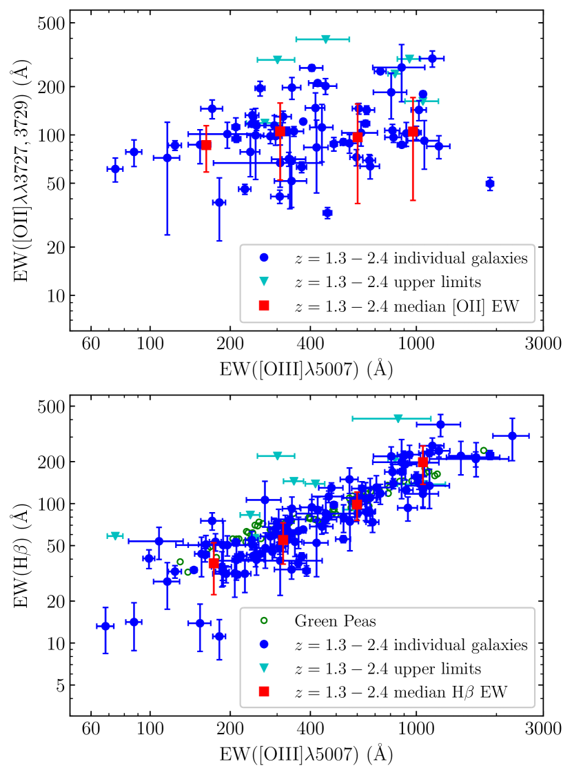
Figure 11: Left Panel: [O II]$\lambda\lambda 3727,3729$ EW as a function of [O III]$\lambda 5007$ EW for the $z=1.3-2.4$ galaxies in our sample. Sources with $>2\sigma$ detections of [O II] are shown by blue circles, while cyan upside-down triangles show the $2\sigma$ upper limits. Red squares present the median [O II] EWs of galaxies in different [O III]$\lambda 5007$ EW bins. Right Panel: H$\beta$ EW as a function of [O III]$\lambda 5007$ EW for the $z=1.3-2.4$ galaxies in our sample. Sources with $>2\sigma$ detections of H$\beta$ are shown by blue circles, while cyan upside-down triangles show the $2\sigma$ upper limits. Red squares present the median H$\beta$ EWs of galaxies in different [O III]$\lambda 5007$ EW bins. For comparison, EWs of Green Peas (Cardamone et al., 2009; Hawley, 2012) are shown by green open circles.

5.3 Implications for JWST observations of $z\simeq 10$ galaxies

The discovery that reionization era systems tend to have strong [O III] emission is important not only for what it tells us about the nature of early galaxies, but also for what it implies about the feasibility of future spectroscopic surveys with JWST. If large equivalent line emission is commonplace, it will be straightforward to build large redshift samples down to faint continuum flux levels. But at the highest redshifts that JWST will hope to probe ($z\gtrsim 10$), the prospects for spectroscopy are not so straightforward. The [O III] line shifts out of the NIRSpec bandpass above $z\simeq 9$, leaving only faint nebular lines in the rest-frame optical ([O II], [Ne III])) and rest-UV (C III], O III], C IV). Over the past few years, there has been considerable efforts invested in the UV lines, revealing equivalent widths that approach $20$ Å for $10-20\%$ of the population (Mainali et al., 2018). In this section, we turn our attention to the EW distribution of the fainter rest-frame optical lines in the extreme emission line population and consider which features are likely to provide the best route to spectroscopic confirmation at $z\gtrsim 9$.

We first consider the feasibility of detecting [O II] emission. Because of the large O32 values expected at high redshift, [O II] is often regarded as prohibitively faint. We have obtained [O II] measurements for 61 galaxies with EW${}_{\rm{[OIII]}\lambda 5007}>225$ Å. In the top panel of Figure 11, we show the dependence of the [O II] doublet EW on the [O III]$\lambda 5007$ EW. For the 55 sources with robust [O II] detections, we measure a median EW of EW${}_{\rm{[OII]}}=103$ Å, with the sample ranging between EW${}_{\rm{[OII]}}=63$ Å (25th percentile) and EW${}_{\rm{[OII]}}=195$ Å (75th percentile), considerably larger than the equivalent widths of the most extreme UV metal line emitters. It is also evident from Figure 11 that there is no strong correlation between [O II] EWs and [O III] EWs at EW${}_{\rm{[OIII]}\lambda 5007}>225$ Å. Given what we know about the [O III] equivalent widths in the reionization-era (e.g. Labbé et al., 2013; Smit et al., 2015), we can use Figure 11 to predict the observability of [O II] at $z\gtrsim 7$. If we consider a $z\simeq 10$ galaxy with the median [O II] EW found in EELGs ($103$ Å), we predict [O II] doublet line fluxes of $2.8\times 10^{-18}$, $1.1\times 10^{-18}$, and $4.5\times 10^{-19}$ erg cm^-2 s^-1 for a $z\simeq 10$ galaxy with apparent magnitudes of $H=26$, $27$, and $28$, respectively. Here we assume a flat continuum in $f_{\nu}$ to extrapolate to the underlying continuum near [O II]. We compute the detectability of [O II] assuming each component of the doublet has a line width typical of the EELGs in our sample (FWHM $=190$ km s^-1). For $R\simeq 1000$ NIRSpec MSA observations with the G395M/F290LP disperser-filter combination, the NIRSpec exposure time calculator predicts the doublet can be detected with S/N $=5$ in 27 minutes (assuming underlying continuum of $H=26$), 2.7 hours ($H=27$), and 16 hrs ($H=28$). This is considerably more efficient than targeting the C III] doublet with NIRSpec. Assuming the most optimistic value for its equivalent width (EW${}_{\rm{CIII]}}\simeq 20$ Å), likely present in only a subset of early galaxies (Mainali et al., 2018), we predict exposure times that are $\gtrsim 6\times$ larger than what is required for detection of [O II].

If the ISM conditions at very high redshift are similar to what we have observed at $z\simeq 0-2$, we expect [Ne III] will be $0.5\times$ the flux of the combined [O II] doublet in the most extreme line emitters. [Ne III] will be narrower than [O II] in the $R\simeq 1000$ grism, allowing it to be detected in just 1 hr ($H=26$) and 6 hrs ($H=27$) for sources with EW${}_{\rm{[NeIII]}}=50$ Å. As recently pointed out in Shapley et al. (2017), deep NIRSpec integrations targeting $z\simeq 10$ galaxies should easily be able to recover both lines in sources with $H\lesssim 27$, providing a unique path toward constraining the ISM conditions in the highest redshift galaxies JWST will probe.

The H$\beta$ line will not be detectable by NIRSpec at $z\gtrsim 10$, as it shifts out of the bandpass at roughly the same redshift as [O III]. But it will serve as an important diagnostic for reionization-era systems. Since H$\beta$ is likely to be among the faintest rest-frame optical lines targeted, it is valuable to know the range of H$\beta$ equivalent widths expected in the extreme emission line population. In the bottom panel of Figure 11, we plot the dependence of the H$\beta$ EW on the [O III]$\lambda 5007$ EW in our spectroscopic sample. The H$\beta$ EW scales with the [O III] EW, with values of EW${}_{\rm{H}\beta}=53$, $98$, and $198$ Å for [O III]$\lambda 5007$ EW bins of EW${}_{\rm{[OIII]}\lambda 5007}=225-450$, $450-800$, and $800-2500$ Å, respectively. As can be seen in Figure 11, the relationship between the H$\beta$ EW and the [O III] EW is very similar for the Green Peas (at EW${}_{\rm{[OIII]}\lambda 5007}>350$ Å), suggesting very little evolution in the trend over $0.3\lesssim z\lesssim 2.4$. If the evolution remains slow at $z\gtrsim 3$, it indicates that H$\beta$ should be detectable in typical ($H\lesssim 27$) reionization-era galaxies with deep ($\lesssim 10$ hr) NIRSpec integrations.

While much attention has recently focused on the rest-UV metal lines, we show here that the fainter rest-frame optical emission lines (i.e., [O II], [Ne III], H$\beta$) are likely to be provide a more efficient route toward spectroscopic confirmation of EELGs at $9\lesssim z\lesssim 12$. For sources that are bright enough ($H\lesssim 26$), the UV nebular lines will complement the picture provided by the rest-frame optical lines, providing unique constraints on the nature of the ionizing sources (e.g. Feltre et al., 2016; Jaskot & Ravindranath, 2016; Mainali et al., 2017; Senchyna et al., 2017; Byler et al., 2018) and the abundance of carbon in the early universe (e.g. Berg et al., 2016). But initial JWST/NIRSpec efforts aimed at building a statistical sample of redshifts for $z\simeq 10$ galaxies are likely to be more successful targeting the observed wavelengths around [O II] and [Ne III].

6 Summary

We report results from a large MMT and Keck spectroscopic survey targeting strong rest-frame optical emission lines in extreme emission line galaxies at high redshift. We have confirmed redshifts of 227 galaxies at $z=1.3-2.4$ with rest-frame [O III]$\lambda 5007$ equivalent widths spanning $225$ Å $<\rm{EW}_{\rm{[OIII]}\lambda 5007}<2500$ Å. This range is chosen to include the average [O III] EW of reionization-era galaxies (EW${}_{\rm{[OIII]}\lambda 5007}\simeq 450$ Å; L13) and the more extreme values (EW${}_{\rm{[OIII]}\lambda 5007}>800$ Å) that characterize most of the known Ly$\alpha$ emitters at $z>7$. By obtaining spectra of similarly intense line emitters at slightly lower redshifts, we hope to gain insight into the range of stellar populations and gas conditions present in the reionization era as well as what distinguishes the Ly$\alpha$ emitting galaxies from the rest of the population at $z\gtrsim 7$.

We fit the broadband continuum SED and emission line fluxes using the BEAGLE tool (Chevallard & Charlot, 2016). The stellar masses implied by the models extend down to $10^{7}\ M_{\odot}$ with a median of $4.9\times 10^{8}\ M_{\odot}$, both well below typical values in the KBSS and MOSDEF surveys. The sSFR distribution extends up to $300$ Gyr^-1 with a median of $17$ Gyr^-1, consistent with very young stellar populations expected after a substantial burst or recent upturn of star formation. We summarize our findings below:

1. The Balmer decrement decreases with increasing [O III] and H$\alpha$ EW, reaching a value close to that expected for case B recombination ($I(\rm{H}\alpha)/I(\rm{H}\beta)=2.90\pm 0.05$) in our composite spectrum of galaxies with EW${}_{\rm{[OIII]}\lambda 5007}=800-2500$ Å. The UV continuum slopes are uniformly blue, with median values of $\beta=-2.04$ for galaxies with EW${}_{\rm{[OIII]}\lambda 5007}>450$ Å. This suggests that both the hot stars and nebular gas are minimally obscured by dust in the most extreme line emitters.

2. We find that the ionizing production efficiency scales with the [O III] and H$\alpha$ EW at high redshift, reaching the largest values ($\log{[\xi^{\rm{HII}}_{\rm{ion}}\ (\rm{erg}^{-1}\ \rm{Hz})]}\simeq 25.6$) in the most intense emitters (EW${}_{\rm{[OIII]}\lambda 5007}>800$ Å). We derive simple scaling laws between the ionizing production efficiency and the [O III] and H$\alpha$ equivalent widths. Comparison to a recent investigation of nearby galaxies (Chevallard et al., 2018) reveals that there is not strong evolution in the link between $\xi^{\star}_{\rm{ion}}$ and the optical lines over $0\lesssim z\lesssim 2$. The trend between the ionizing efficiency and [O III] EW indicates that the extreme line emitters which become common in the reionization era are likely to be very efficient ionizing agents.

3. We discuss the impact of the $\xi^{\star}_{\rm{ion}}-$ [O III] EW relationship on the visibility of Ly$\alpha$ in the reionization era. A large ionizing efficiency results in a larger than average intrinsic Ly$\alpha$ EW, boosting the visibility relative to systems with lower [O III] EW. The detectability is further enhanced by the ionization conditions in the ISM and CGM and the large Ly$\alpha$ velocity offsets associated with massive galaxies. We suggest that the anomalous Ly$\alpha$ success rate in massive galaxies with intense [O III] is likely driven by factors internal to the galaxies and does not necessarily require these objects to sit in the very largest ionized bubbles at these early epochs. Because of their atypical Ly$\alpha$ visibility, massive extreme emission line galaxies may provide a unique probe of the earliest stages of reionization (see Mason et al. 2018b) where substantial neutral fractions (and smaller velocity offsets) make lower mass galaxies very difficult to detect in Ly$\alpha$ (Mason et al., 2018a; Weinberger et al., 2018).

4. We show that two ionization-sensitive line ratios (O32 and Ne3O2) increase with the [O III] EW, revealing extreme ionization conditions in the ISM of the most intense line emitters. In a stacked spectrum of galaxies with EW${}_{\rm{[OIII]}\lambda 5007}=800-2500$ Å, the ionization-sensitive ratios have very large values (O32 $=9.1$ and Ne3O2 $=0.51$) that are commonly associated with LyC leakers at $0\lesssim z\lesssim 2$. We find that very similar O32 and Ne3O2 relationships are also present in Green Pea population, indicating very little redshift evolution over $0.3\lesssim z\lesssim 2.4$ and suggesting a close connection between the [O III] EW and the ionization state of the ISM in the extreme line emitter population.

5. We discuss the O32 $-$ [O III] EW relationship in the context of emerging evidence that large O32 values tend to accompany LyC leakers. Our results demonstrate that the O32 values that appear associated with moderate ($f_{\rm{esc}}\simeq 0.1$) escape fractions (O32 $\gtrsim 6.5$) are most commonly found in EELGs with EW${}_{\rm{[OIII]}\lambda 5007}>760$ Å. The extreme O32 (O32 $>10$) values linked with larger escape fractions ($f_{\rm{esc}}\gtrsim 0.3$) become the norm for galaxies with extremely strong [O III] emission (EW${}_{\rm{[OIII]}\lambda 5007}>1100$ Å). These [O III] EW values are well above the threshold commonly adopted for EELG selections, corresponding to extremely young stellar populations ($\simeq 3-30$ Myr for constant star formation history), consistent with a picture whereby LyC leakage is enhanced during a short window after a burst of star formation.

6. We show that [O II] is likely to be one of the efficient spectroscopic probes at very high redshifts ($z\simeq 10$) where the strongest optical lines are shifted out of the NIRSpec bandpass. In spite of the large O32 values in the strongest line emitters, the median [O II] doublet EW remains fairly large (EW${}_{\rm{[OII]}}\simeq 100$ Å) throughout the EELG population. We show that [O II] is likely to be detected in considerably less exposure time than the strongest of the UV nebular lines (i.e., C III], O III]). [Ne III] should also be readily detectable if Ne3O2 ratios are as large as indicated by our survey.

References

- Abazajian et al. (2009) Abazajian K. N., et al., 2009, ApJS, 182
- Alexander et al. (2003) Alexander D. M., et al., 2003, AJ, 126, 539
- Atek et al. (2018) Atek H., Richard J., Kneib J.-P., Schaerer D., 2018, MNRAS, 479, 5184
- Behroozi et al. (2013) Behroozi P. S., Wechsler R. H., Conroy C., 2013, ApJ, 770, 57
- Berg et al. (2016) Berg D. A., Skillman E. D., Henry R. B. C., Erb D. K., Carigi L., 2016, ApJ, 827, 126
- Bouwens et al. (2015a) Bouwens R. J., et al., 2015a, ApJ, 803, 34
- Bouwens et al. (2015b) Bouwens R. J., Illingworth G. D., Oesch P. A., Caruana J., Holwerda B., Smit R., Wilkins S., 2015b, ApJ, 811, 140
- Brammer et al. (2012) Brammer G. B., et al., 2012, ApJS, 200, 13
- Bruzual & Charlot (2003) Bruzual G., Charlot S., 2003, MNRAS, 344, 1000
- Byler et al. (2018) Byler N., Dalcanton J. J., Conroy C., Johnson B. D., Levesque E. M., Berg D. A., 2018, ApJ, 863, 14
- Caffau et al. (2011) Caffau E., Ludwig H. G., Steffen M., Freytag B., Bonifacio P., 2011, Sol. Phys., 268, 255
- Calzetti et al. (1994) Calzetti D., Kinney A. L., Storchi-Bergmann T., 1994, ApJ, 429, 582
- Calzetti et al. (2000) Calzetti D., Armus L., Bohlin R. C., Kinney A. L., Koornneef J., Storchi-Bergmann T., 2000, ApJ, 533, 682
- Cardamone et al. (2009) Cardamone C., et al., 2009, MNRAS, 399, 1191
- Cardelli et al. (1989) Cardelli J. A., Clayton G. C., Mathis J. S., 1989, ApJ, 345, 245
- Caruana et al. (2014) Caruana J., Bunker A. J., Wilkins S. M., Stanway E. R., Lorenzoni S., Jarvis M. J., Ebert H., 2014, MNRAS, 443, 2831
- Chabrier (2003) Chabrier G., 2003, PASP, 115, 763
- Charlot & Fall (2000) Charlot S., Fall S. M., 2000, ApJ, 539, 718
- Chevallard & Charlot (2016) Chevallard J., Charlot S., 2016, MNRAS, 462, 1415
- Chevallard et al. (2018) Chevallard J., et al., 2018, MNRAS, 479, 3264
- Chilingarian et al. (2015) Chilingarian I., Beletsky Y., Moran S., Brown W., McLeod B., Fabricant D., 2015, PASP, 127, 406
- Civano et al. (2016) Civano F., et al., 2016, ApJ, 819, 62
- Dayal & Ferrara (2018) Dayal P., Ferrara A., 2018, Phys. Rep., 780, 1
- Eldridge et al. (2017) Eldridge J. J., Stanway E. R., Xiao L., McClelland L. A. S., Taylor G., Ng M., Greis S. M. L., Bray J. C., 2017, Publ. Astron. Soc. Australia, 34, e058
- Erb et al. (2016) Erb D. K., Pettini M., Steidel C. C., Strom A. L., Rudie G. C., Trainor R. F., Shapley A. E., Reddy N. A., 2016, ApJ, 830, 52
- Feltre et al. (2016) Feltre A., Charlot S., Gutkin J., 2016, MNRAS, 456, 3354
- Ferland et al. (2013) Ferland G. J., et al., 2013, Rev. Mex. Astron. Astrofis., 49, 137
- Finkelstein et al. (2013) Finkelstein S. L., et al., 2013, Nature, 502, 524
- Finkelstein et al. (2015) Finkelstein S. L., et al., 2015, ApJ, 810, 71
- Fletcher et al. (2018) Fletcher T. J., Robertson B. E., Nakajima K., Ellis R. S., Stark D. P., Inoue A., 2018, preprint, p. arXiv:1806.01741 (arXiv:1806.01741)
- Götberg et al. (2018) Götberg Y., de Mink S. E., Groh J. H., Kupfer T., Crowther P. A., Zapartas E., Renzo M., 2018, A&A, 615, A78
- Grogin et al. (2011) Grogin N. A., et al., 2011, ApJS, 197, 35
- Guseva et al. (2004) Guseva N. G., Papaderos P., Izotov Y. I., Noeske K. G., Fricke K. J., 2004, A&A, 421, 519
- Gutkin et al. (2016) Gutkin J., Charlot S., Bruzual G., 2016, MNRAS, 462, 1757
- Hawley (2012) Hawley S. A., 2012, PASP, 124, 21
- Horne (1986) Horne K., 1986, PASP, 98, 609
- Inoue et al. (2014) Inoue A. K., Shimizu I., Iwata I., Tanaka M., 2014, MNRAS, 442, 1805
- Izotov et al. (2016) Izotov Y. I., Schaerer D., Thuan T. X., Worseck G., Guseva N. G., Orlitová I., Verhamme A., 2016, MNRAS, 461, 3683
- Izotov et al. (2017) Izotov Y. I., Thuan T. X., Guseva N. G., 2017, MNRAS, 471, 548
- Izotov et al. (2018) Izotov Y. I., Worseck G., Schaerer D., Guseva N. G., Thuan T. X., Fricke Verhamme A., Orlitová I., 2018, MNRAS, 478, 4851
- Jaskot & Oey (2013) Jaskot A. E., Oey M. S., 2013, ApJ, 766, 91
- Jaskot & Ravindranath (2016) Jaskot A. E., Ravindranath S., 2016, ApJ, 833, 136
- Kakazu et al. (2007) Kakazu Y., Cowie L. L., Hu E. M., 2007, ApJ, 668, 853
- Kewley et al. (2013) Kewley L. J., Dopita M. A., Leitherer C., Davé R., Yuan T., Allen M., Groves B., Sutherland R., 2013, ApJ, 774, 100
- Kimm & Cen (2014) Kimm T., Cen R., 2014, ApJ, 788, 121
- Koekemoer et al. (2011) Koekemoer A. M., et al., 2011, ApJS, 197, 36
- Kriek et al. (2015) Kriek M., et al., 2015, ApJS, 218, 15
- Labbé et al. (2013) Labbé I., et al., 2013, ApJ, 777, L19
- Laporte et al. (2017) Laporte N., Nakajima K., Ellis R. S., Zitrin A., Stark D. P., Mainali R., Roberts-Borsani G. W., 2017, ApJ, 851, 40
- Levesque & Richardson (2014) Levesque E. M., Richardson M. L. A., 2014, ApJ, 780, 100
- Levesque et al. (2012) Levesque E. M., Leitherer C., Ekstrom S., Meynet G., Schaerer D., 2012, ApJ, 751, 67
- Livermore et al. (2017) Livermore R. C., Finkelstein S. L., Lotz J. M., 2017, ApJ, 835, 113
- Ma et al. (2015) Ma X., Kasen D., Hopkins P. F., Faucher-Giguère C.-A., Quataert E., Kereš D., Murray N., 2015, MNRAS, 453, 960
- Mainali et al. (2017) Mainali R., Kollmeier J. A., Stark D. P., Simcoe R. A., Walth G., Newman A. B., Miller D. R., 2017, ApJ, 836, L14
- Mainali et al. (2018) Mainali R., et al., 2018, MNRAS, 479, 1180
- Maseda et al. (2014) Maseda M. V., et al., 2014, ApJ, 791, 17
- Mason et al. (2018a) Mason C. A., Treu T., Dijkstra M., Mesinger A., Trenti M., Pentericci L., de Barros S., Vanzella E., 2018a, ApJ, 856, 2
- Mason et al. (2018b) Mason C. A., et al., 2018b, ApJ, 857, L11
- Mathis (1986) Mathis J. S., 1986, PASP, 98, 995
- Matthee et al. (2017) Matthee J., Sobral D., Best P., Khostovan A. A., Oteo I., Bouwens R., Röttgering H., 2017, MNRAS, 465, 3637
- McLean et al. (2012) McLean I. S., et al., 2012, in Ground-based and Airborne Instrumentation for Astronomy IV. p. 84460J, doi:10.1117/12.924794
- McLeod et al. (2012) McLeod B., et al., 2012, PASP, 124, 1318
- McLure et al. (2013) McLure R. J., et al., 2013, MNRAS, 432, 2696
- Momcheva et al. (2016) Momcheva I. G., et al., 2016, ApJS, 225, 27
- Naidu et al. (2018) Naidu R. P., Forrest B., Oesch P. A., Tran K.-V. H., Holden B. P., 2018, MNRAS, 478, 791
- Nakajima & Ouchi (2014) Nakajima K., Ouchi M., 2014, MNRAS, 442, 900
- Nakajima et al. (2016) Nakajima K., Ellis R. S., Iwata I., Inoue A. K., Kusakabe H., Ouchi M., Robertson B. E., 2016, ApJ, 831, L9
- Nakajima et al. (2018) Nakajima K., et al., 2018, A&A, 612, A94
- Nandra et al. (2015) Nandra K., et al., 2015, ApJS, 220, 10
- Oesch et al. (2015) Oesch P. A., et al., 2015, ApJ, 804, L30
- Oesch et al. (2018) Oesch P. A., Bouwens R. J., Illingworth G. D., Labbé I., Stefanon M., 2018, ApJ, 855, 105
- Oke & Gunn (1983) Oke J. B., Gunn J. E., 1983, ApJ, 266, 713
- Ono et al. (2012) Ono Y., et al., 2012, ApJ, 744, 83
- Osterbrock & Ferland (2006) Osterbrock D. E., Ferland G. J., 2006, Astrophysics of gaseous nebulae and active galactic nuclei
- Paardekooper et al. (2015) Paardekooper J.-P., Khochfar S., Dalla Vecchia C., 2015, MNRAS, 451, 2544
- Pei (1992) Pei Y. C., 1992, ApJ, 395, 130
- Penston et al. (1990) Penston M. V., et al., 1990, A&A, 236, 53
- Pentericci et al. (2014) Pentericci L., et al., 2014, ApJ, 793, 113
- Petrosian et al. (1972) Petrosian V., Silk J., Field G. B., 1972, ApJ, 177, L69
- Rasappu et al. (2016) Rasappu N., Smit R., Labbé I., Bouwens R. J., Stark D. P., Ellis R. S., Oesch P. A., 2016, MNRAS, 461, 3886
- Reddy et al. (2015) Reddy N. A., et al., 2015, ApJ, 806, 259
- Roberts-Borsani et al. (2016) Roberts-Borsani G. W., et al., 2016, ApJ, 823, 143
- Robertson et al. (2015) Robertson B. E., Ellis R. S., Furlanetto S. R., Dunlop J. S., 2015, ApJ, 802, L19
- Sanders et al. (2016) Sanders R. L., et al., 2016, ApJ, 816, 23
- Sanders et al. (2018) Sanders R. L., et al., 2018, ApJ, 858, 99
- Schenker et al. (2014) Schenker M. A., Ellis R. S., Konidaris N. P., Stark D. P., 2014, ApJ, 795, 20
- Schmidt et al. (1989) Schmidt G. D., Weymann R. J., Foltz C. B., 1989, PASP, 101, 713
- Schmidt et al. (2017) Schmidt K. B., et al., 2017, ApJ, 839, 17
- Senchyna et al. (2017) Senchyna P., et al., 2017, MNRAS, 472, 2608
- Shapley et al. (2016) Shapley A. E., Steidel C. C., Strom A. L., Bogosavljević M., Reddy N. A., Siana B., Mostardi R. E., Rudie G. C., 2016, ApJ, 826, L24
- Shapley et al. (2017) Shapley A. E., et al., 2017, ApJ, 846, L30
- Shivaei et al. (2018) Shivaei I., et al., 2018, ApJ, 855
- Skelton et al. (2014) Skelton R. E., et al., 2014, ApJS, 214, 24
- Smit et al. (2014) Smit R., et al., 2014, ApJ, 784, 58
- Smit et al. (2015) Smit R., et al., 2015, ApJ, 801, 122
- Stanway et al. (2016) Stanway E. R., Eldridge J. J., Becker G. D., 2016, MNRAS, 456, 485
- Stark (2016) Stark D. P., 2016, ARA&A, 54, 761
- Stark et al. (2010) Stark D. P., Ellis R. S., Chiu K., Ouchi M., Bunker A., 2010, MNRAS, 408, 1628
- Stark et al. (2015a) Stark D. P., et al., 2015a, MNRAS, 450, 1846
- Stark et al. (2015b) Stark D. P., et al., 2015b, MNRAS, 454, 1393
- Stark et al. (2017) Stark D. P., et al., 2017, MNRAS, 464, 469
- Stasińska et al. (2015) Stasińska G., Izotov Y., Morisset C., Guseva N., 2015, A&A, 576, A83
- Steidel et al. (2014) Steidel C. C., et al., 2014, ApJ, 795, 165
- Steidel et al. (2016) Steidel C. C., Strom A. L., Pettini M., Rudie G. C., Reddy N. A., Trainor R. F., 2016, ApJ, 826, 159
- Strom et al. (2017) Strom A. L., Steidel C. C., Rudie G. C., Trainor R. F., Pettini M., Reddy N. A., 2017, ApJ, 836, 164
- Tilvi et al. (2016) Tilvi V., et al., 2016, ApJ, 827, L14
- Ueda et al. (2008) Ueda Y., et al., 2008, ApJS, 179, 124
- Vanzella et al. (2016) Vanzella E., et al., 2016, ApJ, 825, 41
- Weinberger et al. (2018) Weinberger L. H., Kulkarni G., Haehnelt M. G., Choudhury T. R., Puchwein E., 2018, MNRAS, 479, 2564
- Wilkins et al. (2016) Wilkins S. M., Feng Y., Di-Matteo T., Croft R., Stanway E. R., Bouwens R. J., Thomas P., 2016, MNRAS, 458, L6
- Wise et al. (2014) Wise J. H., Demchenko V. G., Halicek M. T., Norman M. L., Turk M. J., Abel T., Smith B. D., 2014, MNRAS, 442, 2560
- Xue et al. (2011) Xue Y. Q., et al., 2011, ApJS, 195, 10
- Xue et al. (2016) Xue Y. Q., Luo B., Brandt W. N., Alexander D. M., Bauer F. E., Lehmer B. D., Yang G., 2016, ApJS, 224, 15
- Yang et al. (2017) Yang H., et al., 2017, ApJ, 844, 171
- Zitrin et al. (2015) Zitrin A., et al., 2015, ApJ, 810, L12
- de Barros et al. (2016) de Barros S., et al., 2016, A&A, 585, A51
- van Dokkum et al. (2011) van Dokkum P. G., et al., 2011, ApJ, 743, L15
- van der Wel et al. (2011) van der Wel A., et al., 2011, ApJ, 742, 111