Inferring Complementary Products from Baskets and Browsing Sessions

Abstract.

Complementary products recommendation is an important problem in e-commerce. Such recommendations increase the average order price and the number of products in baskets. Complementary products are typically inferred from basket data. In this study, we propose the BB2vec model. The BB2vec model learns vector representations of products by analyzing jointly two types of data - Baskets and Browsing sessions (visiting web pages of products). These vector representations are used for making complementary products recommendation. The proposed model alleviates the cold start problem by delivering better recommendations for products having few or no purchases. We show that the BB2vec model has better performance than other models which use only basket data.

1. Introduction

Recommender systems in e-commerce are the “must have” technology now. These systems are used by almost all major e-commerce companies. Recommender systems help users to navigate in a vast assortment, discover new items and satisfy various tastes and needs. For online shops, such systems help to convert browsers into buyers (increase conversion rate), do cross-selling, improve users loyalty and retention (Schafer et al., 1999). These effects overall increase the revenue of an e-commerce company and improve customer experience. Worldwide retail e-commerce sales in 2016 are estimated as $1,915 Trillion and will continue to grow by 18%-25% each year . The share of e-commerce in all retail in 2016 is estimated as 8.7% and continues to grow .

The main types of recommendations at e-commerce web site are:

• Personalized: “Products you may like”.

• Non-personalized: “Similar products”, “Complementary products”, ”Popular products”.

Personalized recommendations enjoy a great body of research in recent years (Koren et al., 2009; Rendle et al., 2009; Hu et al., 2008; Deshpande and Karypis, 2004; Linden et al., 2003; Wang and Blei, 2011). In the same time, non-personalized recommendations are less studied. “Similar products” recommendations are typically placed on the product web page. Similar products are substitutes and can be purchased interchangeably. The major goal of similar products recommendation is to persuade a user to purchase by presenting him/her a diverse set of products similar to the original interest. Complementary products can be purchased in addition to each other. For example, an iPhone cover is complementary for iPhone, the second part of a film is complementary to the first part, etc.

When a user already has an intention to purchase - it’s high time for complementary products recommendation. Such recommendations might appear on the product web page, during addition to the shopping cart and the checkout process. In the latter case, recommendations can be based on the whole content of the basket. People naturally tend to buy products in bundles. Complementary products recommendation satisfies this natural need and increases average order price as a consequence.

Online shops try to maximize the revenue by combining all the recommendation scenarios. The significance of recommendations in e-commerce can be illustrated by the following fact: in Amazon, 35% of purchases overall come from products recommendations .

These considerations show that complementary products recommendation is an important scenario. Manual selection of complementary products fails when the number of products in an online shop (or a marketplace) is large and assortment changes quickly. Some companies provide “recommendations as a service” for online shops. These companies deliver real-time recommendations for hundreds and even thousands of shops from various business areas in a fully automated manner.

Machine learning models can solve this problem. There are two principled ways for making complementary products recommendations via machine learning. First way - is to use human assessment to generate the “ground truth” - a set of product-complement pairs. Then some machine learning model can use these pairs as positive examples and build a classifier. This classifier could be applied for identifying complements for all products. The application of this approach is limited for two main reasons. Firstly, it relies on the “ground truth” which should be collected by human assessment. Human assessment is costly and error-prone when the number of products is large and the assortment changes quickly.

An alternative approach is inferring complementary products by analyzing user purchases (baskets) and detecting items which are frequently purchased together. To the best of our knowledge, it is typically done in e-commerce companies by using some heuristical co-occurrence measure (cosine similarity, Jaccard similarity, PMI). The more sophisticated way is to develop a predictive model for such co-occurrences in baskets. In this study, we follow the latter approach.

We make the following contributions in this paper:

1. We propose the statistical model BB2vec. The model itself learns vector representations of products by analyzing jointly two types of data - baskets and browsing sessions (visiting web pages of products). These types of data are always available to any e-commerce company. We apply vector representations learned by the BB2vec model for doing recommendations of complementary products.

2. In experimental studies, we prove that the proposed model BB2vec predicts products which are purchased together better than other methods which rely only on basket data. We show that the BB2vec model alleviates the cold-start problem by delivering better predictions for products having few or no purchases.

3. We show how to make the BB2vecmodel scalable by selecting the specific objective function. It is an important issue since e-commerce company typically has a vast amount of browsing data, much more than basket data.

The source code of our model is publicly available .

2. Related work

After invention of the word2vec model (Mikolov, 2013; Mikolov et al., 2013) which is dedicated to learning of distributed word representations, it was rapidly extended to other kinds of data: sentences and documents (Le and Mikolov, 2014) (doc2vec), products in baskets (Grbovic et al., 2015) (prod2vec, bagged-prod2vec), nodes in graph (Grover and Leskovec, 2016) (node2vec), (Perozzi et al., 2014) (DeepWalk), etc. The original word2vec algorithm in its skip-gram variant proved to solve the weighted matrix factorization problem, where the matrix consists of values of shifted PMI of words (Levy and Goldberg, 2014). The extension of the prod2vec for using items metadata was proposed in (Vasile et al., 2016) (MetaProd2Vec) and for the textual data in (Djuric et al., 2015). Sequences of items selected by a user are modeled in (Guàrdia-Sebaoun et al., 2015) by means of the word2vec-like model. User and item representations learned by their model are applied for making recommendations.

Another associated area of research is multi-relational learning. Multi-relational data is a kind of data when entities (users, items, categories, time moments, etc.) are connected to each other by multiple types of relations (ratings, views, etc.) Collective matrix factorization (Singh and Gordon, 2008) was proposed for relational learning. Each matrix corresponds to a relation between items. Latent vectors of entities are shared. Other variants of models for multi-relational learning are: RESCAL (Nickel et al., 2011), TransE (Bordes et al., 2013), BigARTM (Vorontsov et al., 2015).

In computational linguistics, distributed word representations for two languages could be learned jointly via multi-task learning (Klementiev et al., 2012). This approach improves machine translation.

The importance of learning-to-rank in context of recommendations with implicit feedback is discussed in (Rendle et al., 2009).

2.1. The most similar studies

Sceptre (McAuley et al., 2015) consider two types of relationships between products “being substitutable” and “being complementary”. The “Sceptre” model builds two directed graphs for inferring these two types of relations. As a ground truth for training the model uses recommendation lists crawled from amazon.com. The topic model based on user reviews which also takes into account items taxonomy was used for feature generation. At the top level, the logistic regression did the classification. The application of this approach is limited for two main reasons. Firstly, it relies on “ground truth” which in the real situation should be collected by human assessment. Human assessment is costly and error-prone when the number of products is large. Secondly, it requires rich text descriptions (product reviews) for doing topic modeling.

The prod2vec (Grbovic et al., 2015) model learns product representations from basket data. These representations are used further for doing recommendations of type “Customers who bought $X$ from vendor $V_{1}$ also bought $Y$ from vendor $V_{2}$” which are shown alongside emails in a web interface. Our model is a combination of several prod2vec models which are learned simultaneously with partially shared parameters. We show that this combination has better predictive performance than the single prod2vec model.

P-EMB. Modeling embeddings for exponential family distributions were presented in (Rudolph et al., 2016). The particular model of this family is “Poisson embeddings” (P-EMB) which was applied to model quantities of products in market baskets. Vector representations of products learned by the P-EMB model can be used for inferring substitutable and complementary products. The application of exponential distributions is orthogonal to our research. We consider the BB2vec model can be modified accordingly, i.e., learn several P-EMB models with partially shared parameters instead of prod2vec models.

CoFactor (Liang et al., 2016) improves recommendations from implicit feedback via weighted matrix factorization. The improvement is done by the regularization term which is a factorization problem of a matrix with items co-occurrences (shifted PMI) which is also used in our paper. Our research is different in three main points. Firstly, two parts of the objective (14) come from different sources of data (baskets and browsing sessions), while two parts of the objective in (Liang et al., 2016) (weighted matrix factorization term and regularization term) come from the one kind of data - user-item implicit feedback. Secondly, the objective of the BB2vec is mixed: it includes the skip-gram objective and the matrix factorization one. The procedure of inference is also different - SGD, while (Liang et al., 2016) used coordinate descent. Thirdly, we use pairwise ranking objective and show its benefits.

3. Learning of word representations

The popular word2vec model (Mikolov, 2013; Mikolov et al., 2013) in skip-gram variant learns vector representations of words which are useful for predicting the context of the word in a document. More formally, let $\{w_{1},\ldots,w_{T}\}$ be a sequence of words, $W$ - their vocabulary, the context - a c-sized window of words surrounding $w_{t}$. The likelihood of such model is

(1) $$\frac{1}{T}\sum_{t=1}^{T}\sum_{-c\leq j\leq c,\,j\neq 0}\log P(w_{t+j}|w_{t})$$

The conditional distribution $P(w_{O}|w_{I})$ is defined as

(2) $$P(w_{O}|w_{I})=\frac{\exp{(\mathbf{v}^{\prime}_{w_{O}}}^{T}\mathbf{v}_{w_{I}})}{\sum_{w\in W}\exp({\mathbf{v}^{\prime}_{w}}^{T}\mathbf{v}_{w_{I}})}$$

where $\mathbf{v}_{w},\mathbf{v}^{\prime}_{w}\in\mathbb{R}^{d}$ are input and output representations of words. Together they form $|W|\times d$ matrices $V,V^{\prime}$. Vectors $\mathbf{v}_{w},\mathbf{v}^{\prime}_{w}$ are also known as word embeddings and have many applications in natural language processing, information retrieval, image captioning, etc. Words of similar meaning typically have similar vector representations compared by cosine similarity.

The exact minimization of (1) is computationally hard because of the softmax term. The word2vec algorithm is only concerned with learning high-quality vector representations and it minimizes the more simple negative sampling objective

(3) $$Q^{SG}(V^{\prime},V)=\frac{1}{T}\sum_{t=1}^{T}\sum_{-c\leq j\leq c,\,j\neq 0}L_{neg}(w_{t},w_{t+j})$$

$$L_{neg}(w_{I},w_{O})=\log\sigma({\mathbf{v}^{\prime}_{w_{O}}}^{T}\mathbf{v}_{w_{I}})+\sum_{i=1}^{k}\mathbb{E}_{w_{i}\sim N(w)}\log\sigma(-{\mathbf{v}^{\prime}_{w_{i}}}^{T}\mathbf{v}_{w_{I}})$$

where superscript $SG$ stands for “skip-gram”.

In the negative sampling objective, positive examples $(w_{I},w_{O})$ come from the training data, while in negative samples $(w_{I},w_{i})$ output words $w_{i}$ come from a noise distribution $N(w)$. The noise distribution $N(w)$ is a free parameter which in the original word2vec algorithm is the unigram distribution to the 3/4rd power - $P^{3/4}(w)$.

The word2vec model in skip-gram formulation when $N(w)=P(w)$ implicitly factorizes the matrix of shifted pointwise mutual information (PMI) (Levy and Goldberg, 2014):

(4) $${\mathbf{v}^{\prime}_{w_{i}}}^{T}\mathbf{v}_{w_{j}}=PMI(w_{i},w_{j})-\log k$$

(5) $$PMI(w_{i},w_{j})=\log\left(\frac{n_{ij}/T}{(n_{i}/T)(n_{j}/T)}\right)$$

where $n_{i}$ is a number of times which a word $w_{i}$ occurred in a document, $n_{ij}$ - number of times which two words $w_{i}$, $w_{j}$ occurred together in a c-sized window, $T$ is length of a document. Let

$$Q^{MF}(V^{\prime},V)=\frac{1}{2}\sum_{i,j}(PMI(w_{i},w_{j})-\log k-{\mathbf{v}^{\prime}_{w_{i}}}^{T}\mathbf{v}_{w_{j}})^{2}$$

where superscript $MF$ stands for “matrix factorization”. Solutions of these two problems

(6) $$\mathop{\mathrm{argmin}}_{V^{\prime},V}Q^{SG}(V^{\prime},V)\qquad\mathop{\mathrm{argmin}}_{V^{\prime},V}Q^{MF}(V^{\prime},V)$$

are equal for large enough dimensionality $d$ of vector representations (Levy and Goldberg, 2014).

4. The proposed model

In this section, we describe the proposed BB2vec model. It is a combination of prod2vec models which are fitted with partially shared parameters (multi-task learning).

4.1. Product recommendations with prod2vec

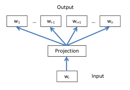
Figure 1. Skip-gram model, basket/session = $\{w_{1},w_{2},\ldots,w_{n}\}$

The original word2vec model can be easily applied to other domains by redefining the “context” and the “word”. Some examples include modeling products in baskets (Grbovic et al., 2015), nodes in graph (Grover and Leskovec, 2016; Perozzi et al., 2014), sequences of items selected by users (Guàrdia-Sebaoun et al., 2015), etc.

Particulary, the prod2vec model (Grbovic et al., 2015) assumes the following likelihood

(7) $$\sum_{B\in\mathfrak{B}}\sum_{w_{t}\in B}\;\sum_{-c\leq j\leq c,\,j\neq 0}\log P(w_{t+j}|w_{t})$$

where $\mathfrak{B}$ is a set of baskets.

The context $C$ in the original word2vec model (1) is a c-sized windows since it is tailored for long text sequences. In our study, we analyze shorter sequences like baskets or e-commerce browsing sessions. We use a modified likelihood

(8) $$\sum_{B\in\mathfrak{B}}\sum_{\begin{subarray}{c}w_{I},w_{O}\in B\\ w_{I}\neq w_{O}\end{subarray}}\log P(w_{O}|w_{I}).$$

where context is the full basket, except an input product, independently of its size (see fig. 1). This eliminates the need for selecting the window size.

Consider the product $k$. By definition, complementary products are frequently purchased together and have high conditional probability $P(m\,|\,k)$ .

The most simple way to estimate the conditional probability $P(m\,|\,k)$ is by empirical frequencies (co-counting). Let $n_{k}$ be a number of baskets with item $k$, $n_{mk}$ - number of baskets with both items $k$ and $m$. Here and after we assume for simplicity that an item might appear in a basket/session only once. Then

$$P(m\,|\,k)\approx\frac{n_{mk}}{n_{k}}$$

However, counts $n_{mk},n_{k}$ are noisy for products having few purchases.

The prod2vec model can generate recommendations of complementary products without co-counting. Given the vector representations of products $V,V^{\prime}$, complementary products for the item $k$ could be inferred by selecting items $m$ with a high score ${\mathbf{v}^{\prime}_{m}}^{T}\mathbf{v}_{k}$ since $P(m\,|\,k)\sim\exp({\mathbf{v}^{\prime}_{m}}^{T}\mathbf{v}_{k})$ (2). The connection of representations $V,V^{\prime}$ to the conditional distribution $P(m\,|\,k)$ in the data is an intrinsic limitation of the prod2vec model. In the next section, we will show how to overcome this limitation by means of the multi-task learning and the specific objective function.

4.2. Multi-task learning

1

2

3

4

Input : Tasks $T_{i}$, weights $\lambda_{i}$, $i=1,\ldots,K$

5

6for $j=1,\ldots,L$ do

7       Initialize elements of matrices $V_{j},V^{\prime}_{j}$ with $N(0,0.1)$

8      

9

10$W=\sum_{i=1}^{K}\lambda_{i}$

11 $\xi$ - random variable having categorical distribution $Cat(\frac{\lambda_{1}}{W},\ldots,\frac{\lambda_{K}}{W})$

12repeat until convergence 

13       Sample $i$ from $\xi$     (select the task $T_{i}$)

14       Sample object-context pair $(w_{I},w_{O})$ from the task $T_{i}$

15       for $m=1,\ldots,{\mid W\mid},\,n=1,\ldots,d$ do

16            

$$V_{g(i)}^{m,n}\leftarrow V_{g(i)}^{m,n}-\eta^{m,n}\frac{\partial L_{neg}(w_{I},w_{O})}{\partial V_{g(i)}^{m,n}}$$

$${V^{\prime}}_{g^{\prime}(i)}^{m,n}\leftarrow{V^{\prime}}_{g^{\prime}(i)}^{m,n}-{\eta^{\prime}}^{m,n}\frac{\partial L_{neg}(w_{I},w_{O})}{\partial{V^{\prime}}_{g^{\prime}(i)}^{m,n}}$$

where learning rates $\eta^{m,n},{\eta^{\prime}}^{m,n}$ are calculated by the AdaGrad rule (Duchi et al., 2011).

17      

18

Output : $V_{j},V^{\prime}_{j}$, for $j=1\ldots L$

Algorithm 1 Multi-task learning of representations

Assume that multiple types of data contain same objects. E-commerce data naturally have such data types: browsing sessions, baskets, product comparisons, search results, etc. Let {$T_{1},\ldots,T_{K}\}$ be a list of such data types. For each data type $T_{i}$, one may fit the prod2vec model and infer latent representations of items $V_{i},V^{\prime}_{i}$ by solving the problem

$$\min_{V_{i}^{\prime},V_{i}}Q^{SG}_{T_{i}}(V^{\prime}_{i},V_{i})$$

We will refer to each learning problem as a task.

Then we assume that some representations are shared and the total number of distinct representations $L$ is less then the number of tasks $K$. The functions $g^{\prime},g:\{1,\ldots,K\}\to\{1,\ldots,L\}$ define which matrices are shared between tasks. For example, if $g(i)=g(j)$ then the input representations $V$ of objects in the tasks $T_{i},T_{j}$ are shared. We come to the following multi-task learning problem

(9) $$\min_{\begin{subarray}{c}V_{j}^{\prime},V_{j}\\ j=1\ldots L\end{subarray}}\sum_{i=1}^{K}\lambda_{i}Q^{SG}_{T_{i}}(V_{g^{\prime}(i)}^{\prime},V_{g(i)})$$

Algorithm 1 describes a procedure for solving the problem (9). At the top level, the Algorithm 1 selects a task $T_{i}$ with probability proportional to its weight $\lambda_{i}$. Then a random object-context pair is sampled and representations of items $V_{g(i)},V^{\prime}_{g^{\prime}(i)}$ are updated via SGD with AdaGrad learning rates.

4.3. Motivation of multi-task representations learning

Optimizing the objective (9) is an example of multi-task learning (MTL). Multi-task learning is about solving several related learning problems simultaneously. The problems with not enough data may benefit from coupling parameters with other problems. However, multi-task learning may worsen a predictive performance. Avoiding it requires choosing a proper way of binding tasks together.

Consider a problem of complementary items recommendation in e-commerce. By definition, complementary items are those which could be purchased in addition to each other. As we explained in the section 4.1, the prod2vec model learns representations $V_{B}^{\prime},V_{B}$ of products by solving the problem

(10) $$V^{\prime}_{B},V_{B}=\mathop{\mathrm{argmin}}_{V^{\prime},V}Q^{SG}_{baskets}(V^{\prime},V)$$

and products having high score ${\mathbf{v}^{\prime}_{m,B}}^{T}\mathbf{v}_{k,B}$ are complementary.

This predictive model can be improved further by analyzing another source of data - browsing sessions. The probability of purchase in a session is typically 1%-5%. Thus, an online shop has much more browsing data then purchasing data. The prod2vec model can learn product representations from browsing data by solving the problem

(11) $$V^{\prime}_{S},V_{S}=\mathop{\mathrm{argmin}}_{V^{\prime},V}Q^{SG}_{brows.}(V^{\prime},V)$$

It is generally accepted that products which are frequently viewed in the same sessions are similar. Let $S$ be a browsing session. Two items $m,k$ having high conditional probability $P(m\in S\,|\,k\in S)$ are similar.

We conclude that conditional distributions $P(m\in B\,|\,k\in B)$ and $P(m\in S\,|\,k\in S)$ are different which leads to different representations $V^{\prime}_{B},V_{B}$ vs. $V^{\prime}_{S},V_{S}$. In the same time, the general property of the prod2vec and other extensions of the word2vec model is that similar objects have similar representations.

In our research, we use the specific objective function for learning product representations where input $V_{B}$ and output $V^{\prime}_{B}$ representations are shared separately between tasks

(12) $$\min_{V^{\prime}_{B},V_{B},V^{\prime}_{S},V_{S}}Q^{SG}_{bask.}(V^{\prime}_{B},V_{B})+\lambda\left(Q^{SG}_{browse}(V^{\prime}_{S},V_{B})+Q^{SG}_{browse}(V^{\prime}_{B},V_{S})\right)$$

Addition of $\lambda Q^{SG}_{browse}(V^{\prime}_{S},V_{B})$ forces $V_{B}$ to be a good input representation for modeling similar products, particularly forcing representations of similar products $V_{B}$ to be close. The same holds for output representation $V^{\prime}_{B}$ because of the term $\lambda Q^{SG}_{browse}(V^{\prime}_{B},V_{S})$.

4.4. Ranking

Learning of vector representations in skip-gram variant (3) is considered to be a binary classification problem when positive object-context examples are drawn from the training dataset, and negative examples are drawn from the noise distribution. Since our final goal is to use representations for generating top-N recommendations one may reformulate the problem as learning to rank. We can easily transform a skip-gram negative sampling problem (3) into the pairwise ranking problem.

In this formulation we treat $w_{I}$ as a query item and force our model to give positive example $w_{O}$ higher rank than negative examples $w_{i}\sim N(w)$. The value ${\mathbf{v}^{\prime}_{w_{i}}}^{T}\mathbf{v}_{w_{I}}$ is the ranking score:

(13) $$Q^{SG}(V^{\prime},V)=\sum_{\begin{subarray}{c}w_{I},w_{O}\in B\\ w_{I}\neq w_{O}\end{subarray}}\;\sum_{i=1}^{k}\mathbb{E}_{w_{i}\sim N(w)}\log(\sigma(({\mathbf{v}^{\prime}_{w_{O}}}^{T}-{\mathbf{v}^{\prime}_{w_{i}}}^{T})\mathbf{v}_{w_{I}}))$$

We can show (see Appendix A) that optimizing (13) with respect to $V,V^{\prime}$ in the general case $N(w)=P^{\alpha}(w)$ leads to the solution

$$(\mathbf{v}^{\prime}_{r}-\mathbf{v}^{\prime}_{m})^{T}\mathbf{v}_{k}=\log\left(\frac{P(r\,|\,k)}{P^{\alpha}(r)}\right)-\log\left(\frac{P(m\,|\,k)}{P^{\alpha}(m)}\right)$$

Thus, if ${\mathbf{v}^{\prime}_{r}}^{T}\mathbf{v}_{k}>{\mathbf{v}^{\prime}_{m}}^{T}\mathbf{v}_{k}$ then $\frac{P(r\,|\,k)}{P^{\alpha}(r)}>\frac{P(m\,|\,k)}{P^{\alpha}(m)}$. Interestingly, the number of negative samples $k$ vanished and doesn’t introduce a shift like in the classification setting (5). For ranking, it can be considered as a hyperparameter of training. We will use further the learning to rank (13) variant of negative sampling problem.

4.5. Improving computational performance of the BB2vec model

Since there are much more browsing data than basket data, solving the skip-gram problems $Q^{SG}_{browse}(\cdot)$ requires much more SGD updates in the Algorithm 1 than in the original problem $Q^{SG}_{bask.}(\cdot)$ and significantly slows down the program.

The software implementation of the BB2vec model solves matrix factorization problems $Q^{MF}_{browse}(\cdot)$ instead of the skip-gram problems $Q^{SG}_{browse}(\cdot)$ for browsing sessions since their solutions are asymptotically equal (6). As a result, the software implementation optimizes the following objective

(14) $$\min_{V^{\prime}_{B},V_{B},V^{\prime}_{S},V_{S}}Q^{SG}_{bask.}(V^{\prime}_{B},V_{B})+\lambda\left(Q^{MF}_{browse}(V^{\prime}_{S},V_{B})+Q^{MF}_{browse}(V^{\prime}_{B},V_{S})\right)$$

The matrix factorization problems are solved by the stochastic matrix factorization (Koren et al., 2009) with AdaGrad learning rates (Duchi et al., 2011).

The complexity of one epoch for solving $Q^{SG}_{browse}(\cdot)$ is

$$O(\#sessions\cdot avg.session\,size\cdot\#neg.samples\cdot d)$$

while the complexity of one epoch of the stochastic matrix factorization of the shifted $PMI$ matrix is

$$O(\#entries\;in\;SMPI\;matrix\cdot d)$$

For our datasets, the complexity of solving the stochastic matrix factorization of the shifted $PMI$ matrix is roughly $10^{3}$ times less.

5. Experiments

In computational experiments, we compared different models for complementary products recommendation. We measured how well each model predicts products which are purchased together in baskets at the hold-out data.

5.1. Datasets

Table 1. Datasets.

Dataset	Sessions	Baskets			Items
		train	val/test	w/ $\geq 2$ items	total	w/o purch. at train
RecSys’15	9,249,729	346,554	74,161	49%	7226	0%
RecSys’15 - 10%	9,249,729	34,753	74,161	49%	7226	17%
CIKM’16	310,486	9380	2063	19%	11244	11%
CIKM’16, Categories	310,486	9380	2063	17%	750	5%

To evaluate the performance of the BB2vec and compare it with baselines we used 4 datasets with user behaviour log on e-commerce web sites (see Table 1):

1. RecSys’15 - the dataset from the ACM RecSys 2015 challenge . The challenge data has two main parts: clicks on items (equivalent to visiting products web pages) and purchases. We consider a basket to be a set of items purchased in a session. Products with less then 10 purchases in the whole dataset were removed. We randomly split sessions to train, validation and test in the proportion 70% / 15% / 15%.

2. RecSys’15 - 10% - is the modification of the RecSys’15 dataset. The only difference is that the training dataset was replaced by it’s 10% subsample, while validation and test were left unchanged.

3. CIKM’16 - is the dataset from CIKM Cup 2016 Track 2 . We took browsing log (product page views) and transactions (baskets). We randomly split sessions to train, validation and test in proportion 70% / 15% / 15%. All baskets have session identifier and were split accordingly.

4. CIKM’16, Categories - is a modifications of CIKM’16 dataset. Since CIKM’16 dataset is very sparse, we replaced product identifiers with their category identifiers. The number of distinct categories is much less than the number of products. Thus, dataset becomes denser.

Finally, for each dataset, we left at test and validation parts only products having at least one purchase or a view at the training dataset. Otherwise, methods under considerations can’t learn vector representations for such products. All the purchase counts and the view counts were binarized.

In computational experiments, PMI matrices were calculated using browsing data from train datasets only. For RecSys’15, RecSys’15, 10% datasets the cells of PMI matrix having $n_{ij}\geq 10$ were kept. For CIKM’16, CIKM’16 Category the cells of PMI matrix having $n_{ij}\geq 3$ were kept.

5.2. Evaluation

We evaluated the performance of the models by predicting items which are purchased together in baskets at hold-out data. We used two measures: average HitRate@K and NDCG@K. For each basket $B$, consider all distinct pairs of items $k,m\in B$. The goal is to predict the second item $m$ in the pair given the first one $k$ (query item). Denote $L_{k}$, a list of length K with complementary items recommendations for the query item $k$.

Then

$$\text{HitRate@K}=[m\in L_{k}]$$

$$\text{NDCG@K}=\frac{[m\in L_{k}]}{\log_{2}(pos(m,L_{k})+1)}$$

where $[\cdot]$ is an indicator function, $pos(m,L_{k})$ is the position of item $m$ in the list $L_{k}$. These performance measures are averaged

• over all distinct pairs of items $(k,m)$ in all the baskets;

• or over a subset of pairs of items $(k,m)$ with query item $k$ having a particular number of purchases at the training dataset.

5.3. Models

Table 2. Experimental results.

Method	CIKM’16				CIKM’16, Categories
	HitRate@		NDCG@		HitRate@		NDCG@
	10	50	10	50	10	50	10	50
Popularity	0.006	0.047	0.006	0.024	0.201	0.482	0.174	0.305
Co-counting	0.015	0.016	0.023	0.024	0.391	0.477	0.531	0.574
Prod2Vec	0.018	0.021	0.025	0.026	0.322	0.510	0.467	0.547
BB2vec, class.	0.027	0.039	0.036	0.042	0.354	0.609	0.483	0.598
BB2vec, ranking	0.029	0.077	0.029	0.051	0.430	0.659	0.559	0.665

Method	RecSys’15				RecSys’15, 10%
	HitRate@		NDCG@		HitRate@		NDCG@
	10	50	10	50	10	50	10	50
Popularity	0.036	0.127	0.031	0.071	0.036	0.128	0.031	0.072
Co-counting	0.383	0.569	0.475	0.561	0.333	0.453	0.419	0.475
Prod2Vec	0.379	0.585	0.461	0.557	0.329	0.411	0.400	0.440
BB2vec, class.	0.383	0.593	0.464	0.562	0.351	0.505	0.420	0.493
BB2vec, ranking	0.383	0.597	0.465	0.564	0.356	0.559	0.425	0.519

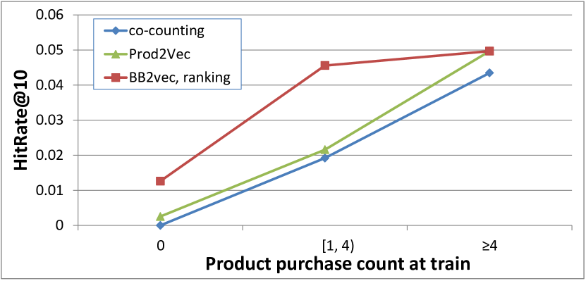
(a) CIKM’16

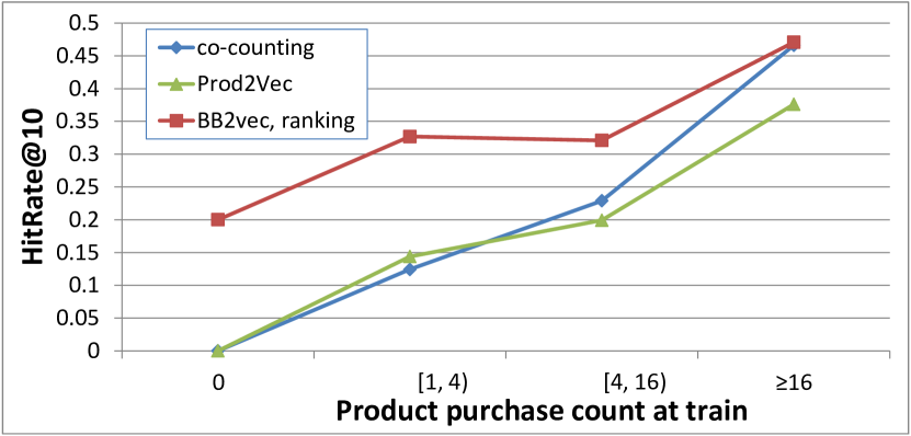
(b) CIKM’16, Categories

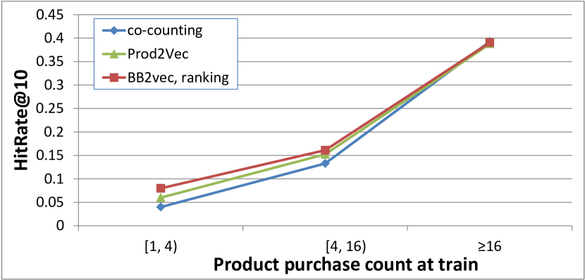
(c) ACM RecSys’15

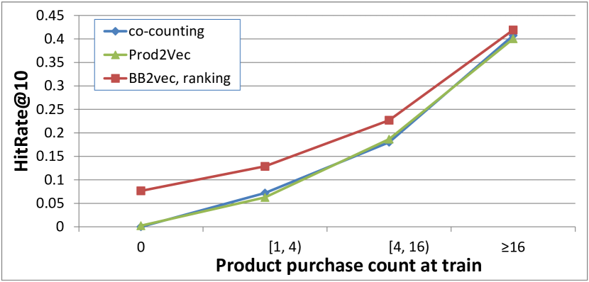
(d) ACM RecSys’15, 10%

Figure 2. Model performance vs. product purchase count

In computational experiments, we evaluated the performance of the proposed BB2vec model. This model learns vector representations of products from baskets and browsing sessions by optimizing the objective (12). We evaluated two variants: with classification (BB2vec, class.) and ranking (BB2vec, ranking) objectives.

We compared the proposed BB2vec model with the following baselines:

1. Popularity: items are sorted by purchases count at train.

2. Co-counting: for the query item $k$ top items with joint purchases $n_{km}$ are selected. If for two items $m,r:$ $n_{mk}=n_{rk}$ then the item with larger purchase count had higher rank.

3. prod2vec. We implemented the prod2vec algorithm (Grbovic et al., 2015) and fit item representations from basket data. The context in the skip-gram objective always was all items in a basket except the input item. It is equivalent to setting window size in prod2vec to the size of the largest basket. Thus the model optimizes the objective (10).

Validation datasets were used for early stopping. The initial learning rate in AdaGrad was set to $0.05$. The number of negative samples was set to 20. All hyperparameters of the methods (latent vectors dimensionality, mixing parameters $\lambda$) of were tuned for maximizing HitRate@10 at validation datasets and final results in the table 2 are calculated at test datasets (see Appendix B). In the prod2vec and BB2vec models negative items were sampled uniformly.

For the predictive models prod2vec and BB2vec we used matrices $V^{\prime}_{B},V_{B}$ for generating recommendations. Given a query item $k$, top N items by the score ${\mathbf{v}^{\prime}_{m,B}}^{T}\mathbf{v}_{k,B}$ are selected.

5.4. Results

Firstly, we analyze the overall performance of the methods under evaluation. Table 2 show the average HitRate and NDCG over test datasets. We conclude that the proposed BB2vec model has the best predictive performance among almost all the datasets and performance measures. The difference between the models BB2vec, class. vs. prod2vec is the effect of learning of shared product representations for both purchases and browsing sessions, instead of representations for purchases only. The variant with the learning-to-rank objective BB2vec, rank. is better than the classification one BB2vec, class. The gap between BB2vec and other models is the most sound at sparse datasets CIKM’16, CIKM’16 Categories, RecSys’15 10%.

Secondly, we analyze in how the BB2vec model alleviates the cold start problem. Fig. 2 shows the breakdown of average HitRate@10 by product purchase count at train dataset. The BB2vec model performs better for products having few or no purchases. In the same time, for products having enough purchases ($\geq 4$ for CIKM dataset, $\geq 16$ for other datasets) the BB2vec does not generate better recommendations than other models. The notorious feature of the BB2vec model is that is can make recommendations for products with no purchases at the training set. We conclude that the improvement of the overall performance comes from better recommendations for products having few or no purchases at the training dataset.

6. Conclusions

In this paper, we proposed the BB2vec model for complementary products recommendation in e-commerce. The model learns product representations by processing simultaneously two kinds of data - baskets and browsing sessions which are the very basic ones and always available to any e-commerce company. Despite the large amount of browsing sessions, the learning algorithm is computationally scalable.

The predictive performance of the BB2vec model is better than the performance of state-of-the-art models which rely solely on basket data. We show that the improvement comes from better recommendations for products having few or no purchases. Thus, the proposed model alleviates the cold start problem. Unlike other models, the BB2vec model can generate recommendations for products having no purchases.

Our model can be extended in two ways. Firstly, one can use other algorithms as tasks in the multi-task objective, for example the P-EMB model. Secondly, our model can be extended to handle items metadata.

Appendix A Ranking loss function

Consider a basket $B$, input item $k\in B$, output item $m\in B$ and negative samples $r\sim P^{\alpha}(w)$. Then the negative sampling objective for learning-to-rank variant equals

$$Q^{SG}(V,V^{\prime}) =\sum_{B\in\mathcal{B}}\sum_{\begin{subarray}{c}k,m\in B\\ k\neq m\end{subarray}}\mathbb{E}_{r\sim P^{\alpha}(w)}\log(1+\exp((\mathbf{v}^{\prime}_{r}-\mathbf{v}^{\prime}_{m})^{T}\mathbf{v}_{k}))$$

Let $P(k,m)$ be the empirical distribution of item pairs $(k,m)$ in the baskets $\mathcal{B}$, $a_{rmk}=(\mathbf{v}^{\prime}_{r}-\mathbf{v}^{\prime}_{m})^{T}\mathbf{v}_{k}$, $N=\sum_{B\in\mathcal{B}}|\{k,m\in B,k\neq m\}|$. Then

$$\frac{1}{N}Q^{SG}(V,V^{\prime}) =\sum_{k,m,r}P(k,m)P^{\alpha}(r)\log(1+\exp((\mathbf{v}^{\prime}_{r}-\mathbf{v}^{\prime}_{m})^{T}\mathbf{v}_{k}))$$

$$=\sum_{k,m,r}P(k)P(m|k)P^{\alpha}(r)\log(1+\exp((\mathbf{v}^{\prime}_{r}-\mathbf{v}^{\prime}_{m})^{T}\mathbf{v}_{k}))$$

$$=\sum_{k,m,r}P(k)P(m|k)P^{\alpha}(r)\log(1+\exp(a_{rmk}))$$

$$=\frac{1}{2}\sum_{k,m,r}P(k)P(m|k)P^{\alpha}(r)\log(1+\exp(a_{rmk}))$$

$$\qquad+P(k)P(r|k)P^{\alpha}(m)\log(1+\exp(-a_{rmk}))$$

$$=\frac{1}{2}\sum_{k,m,r}P(k)f(a_{rmk})$$

here we defined the function

$$f(a)=P(m|k)P^{\alpha}(r)\log(1+\exp(a))+P(r|k)P^{\alpha}(m)\log(1+\exp(-a))$$

and used the identity $a_{mrk}=-a_{rmk}$.

The derivative of $f(a)$ is

$$f^{\prime}(a)=\frac{1}{1+\exp(a)}(P(m|k)P^{\alpha}(r)\exp(a)-P(r|k)P^{\alpha}(m))$$

By solving the equation $f^{\prime}(a_{rmk})=0$ we obtain

$$a_{rmk}=\log\left(\frac{P(r|k)}{P^{\alpha}(r)}\right)-\log\left(\frac{P(m|k)}{P^{\alpha}(m)}\right)$$

Recalling than $a_{rmk}=(\mathbf{v}^{\prime}_{r}-\mathbf{v}^{\prime}_{m})^{T}\mathbf{v}_{k}$ we conclude that ranking by the score ${\mathbf{v}^{\prime}_{r}}^{T}\mathbf{v}_{k}$ is equivalent to the ranking by $P(r|k)/P^{\alpha}(r)$.

Appendix B Best hyperparameters of the models

Dataset /  Model	prod2vec	BB2vec
CIKM’16	$d=400$	$d=100,\lambda=2$
CIKM’16 Categories	$d=200$	$d=100,\lambda=8$
RecSys’15	$d=100$	$d=200,\lambda=8$
RecSys’15, 10%	$d=100$	$d=400,\lambda=32$

References

- (1)
- Bordes et al. (2013) Antoine Bordes, Nicolas Usunier, Jason Weston, and Oksana Yakhnenko. 2013. Translating Embeddings for Modeling Multi-Relational Data. Advances in NIPS 26 (2013), 2787–2795. arXiv:arXiv:1011.1669v3
- Deshpande and Karypis (2004) Mukund Deshpande and George Karypis. 2004. Item-based top-n recommendation algorithms. ACM Transactions on Information Systems (TOIS) 22, 1 (2004), 143–177.
- Djuric et al. (2015) Nemanja Djuric, Hao Wu, Vladan Radosavljevic, Mihajlo Grbovic, and Narayan Bhamidipati. 2015. Hierarchical neural language models for joint representation of streaming documents and their content. In Proceedings of the 24th International Conference on World Wide Web. International World Wide Web Conferences Steering Committee, 248–255.
- Duchi et al. (2011) John Duchi, Elad Hazan, and Yoram Singer. 2011. Adaptive subgradient methods for online learning and stochastic optimization. Journal of Machine Learning Research 12, Jul (2011), 2121–2159.
- Grbovic et al. (2015) Mihajlo Grbovic, Vladan Radosavljevic, Nemanja Djuric, Narayan Bhamidipati, Jaikit Savla, Varun Bhagwan, and Doug Sharp. 2015. E-commerce in Your Inbox : Product Recommendations at Scale Categories and Subject Descriptors. In SIGKDD 2015: Proceedings of the 21th ACM SIGKDD International Conference on Knowledge Discovery and Data Mining. 1809–1818. arXiv:1606.07154
- Grover and Leskovec (2016) Aditya Grover and Jure Leskovec. 2016. node2vec: Scalable feature learning for networks. In Proceedings of the 22nd ACM SIGKDD International Conference on Knowledge Discovery and Data Mining. ACM, 855–864.
- Guàrdia-Sebaoun et al. (2015) Elie Guàrdia-Sebaoun, Vincent Guigue, and Patrick Gallinari. 2015. Latent trajectory modeling: A light and efficient way to introduce time in recommender systems. In Proceedings of the 9th ACM Conference on Recommender Systems. ACM, 281–284.
- Hu et al. (2008) Yifan Hu, Yehuda Koren, and Chris Volinsky. 2008. Collaborative filtering for implicit feedback datasets. In Data Mining, 2008. ICDM’08. Eighth IEEE International Conference on. Ieee, 263–272.
- Klementiev et al. (2012) Alexandre Klementiev, Ivan Titov, and Binod Bhattarai. 2012. Inducing crosslingual distributed representations of words. (2012).
- Koren et al. (2009) Yehuda Koren, Robert Bell, and Chris Volinsky. 2009. Matrix factorization techniques for recommender systems. Computer 42, 8 (2009).
- Le and Mikolov (2014) Qv Le and Tomas Mikolov. 2014. Distributed Representations of Sentences and Documents. International Conference on Machine Learning - ICML 2014 32 (2014), 1188–1196. arXiv:1405.4053
- Levy and Goldberg (2014) Omer Levy and Yoav Goldberg. 2014. Neural Word Embedding as Implicit Matrix Factorization. In Advances in Neural Information Processing Systems (NIPS). 2177–2185. arXiv:1405.4053
- Liang et al. (2016) Dawen Liang, Jaan Altosaar, Laurent Charlin, and David M. Blei. 2016. Factorization meets the item embedding: regularizing matrix factorization with item co-occurrance. In ACM RecSys. arXiv:arXiv:1602.05561v1
- Linden et al. (2003) Greg Linden, Brent Smith, and Jeremy York. 2003. Amazon.com recommendations: Item-to-item collaborative filtering. IEEE Internet Computing 7, 1 (2003), 76–80. arXiv:69
- McAuley et al. (2015) Julian McAuley, Rahul Pandey, and Jure Leskovec. 2015. Inferring networks of substitutable and complementary products. In Proceedings of the 21th ACM SIGKDD International Conference on Knowledge Discovery and Data Mining. ACM, 785–794.
- Mikolov (2013) Tomas Mikolov. 2013. Learning Representations of Text using Neural Networks (Slides). In NIPS Deep Learning Workshop. 1–31. arXiv:arXiv:1310.4546v1
- Mikolov et al. (2013) Tomas Mikolov, Greg Corrado, Kai Chen, and Jeffrey Dean. 2013. Efficient Estimation of Word Representations in Vector Space. Proceedings of the International Conference on Learning Representations (ICLR 2013) (2013), 1–12. arXiv:arXiv:1301.3781v3
- Nickel et al. (2011) Maximilian Nickel, Volker Tresp, and Hans-Peter Kriegel. 2011. A three-way model for collective learning on multi-relational data. In Proceedings of the 28th international conference on machine learning (ICML-11). 809–816.
- Perozzi et al. (2014) Bryan Perozzi, Rami Al-Rfou, and Steven Skiena. 2014. Deepwalk: Online learning of social representations. In Proceedings of the 20th ACM SIGKDD international conference on Knowledge discovery and data mining. ACM, 701–710.
- Rendle et al. (2009) Steffen Rendle, Christoph Freudenthaler, Zeno Gantner, and Lars Schmidt-Thieme. 2009. BPR: Bayesian Personalized Ranking from Implicit Feedback. In Proceedings of the Twenty-Fifth Conference on Uncertainty in Artificial Intelligence. 452–461. arXiv:1205.2618
- Rudolph et al. (2016) Maja Rudolph, Francisco Ruiz, Stephan Mandt, and David Blei. 2016. Exponential Family Embeddings. In Nips. 478–486. arXiv:1608.00778
- Schafer et al. (1999) J Ben Schafer, Joseph Konstan, and John Riedl. 1999. Recommender systems in e-commerce. In Proceedings of the 1st ACM conference on Electronic commerce. ACM, 158–166.
- Singh and Gordon (2008) Ajit P Singh and Geoffrey J Gordon. 2008. Relational learning via collective matrix factorization. In Proceedings of the 14th ACM SIGKDD international conference on Knowledge discovery and data mining. ACM, 650–658.
- Vasile et al. (2016) Flavian Vasile, Elena Smirnova, and Alexis Conneau. 2016. Meta-Prod2Vec - Product Embeddings Using Side-Information for Recommendation. 0–7. arXiv:1607.07326
- Vorontsov et al. (2015) Konstantin Vorontsov, Oleksandr Frei, Murat Apishev, Peter Romov, Marina Suvorova, and Anastasia Yanina. 2015. Non-bayesian additive regularization for multimodal topic modeling of large collections. In Proceedings of the 2015 Workshop on Topic Models: Post-Processing and Applications. ACM, 29–37.
- Wang and Blei (2011) Chong Wang and David M Blei. 2011. Collaborative topic modeling for recommending scientific articles. In Proceedings of the 17th ACM SIGKDD international conference on Knowledge discovery and data mining. ACM, 448–456.