Fast real-time time-dependent hybrid functional calculations with the parallel transport gauge and the adaptively compressed exchange formulation

Abstract

We present a new method to accelerate real time-time dependent density functional theory (rt-TDDFT) calculations with hybrid exchange-correlation functionals. In the context of a large basis set such as planewaves and real space grids, the main computational bottleneck for large scale calculations is the application of the Fock exchange operator to the time-dependent orbitals. Our main goal is to reduce the frequency of applying the Fock exchange operator, without loss of accuracy. We achieve this by combining the recently developed parallel transport (PT) gauge formalism [Jia et al, arXiv:1805.10575] and the adaptively compressed exchange operator (ACE) formalism [Lin, J. Chem. Theory Comput. 12, 2242, 2016]. The PT gauge yields the slowest possible dynamics among all choices of gauge. When coupled with implicit time integrators such as the Crank-Nicolson (CN) scheme, the resulting PT-CN scheme can significantly increase the time step from sub-attoseconds to $10-100$ attoseconds. At each time step $t_{n}$, PT-CN requires the self-consistent solution of the orbitals at time $t_{n+1}$. We use ACE to delay the update of the Fock exchange operator in this nonlinear system, while maintaining the same self-consistent solution. We verify the performance of the resulting PT-CN-ACE method by computing the absorption spectrum of a benzene molecule and the response of bulk silicon systems to an ultrafast laser pulse, using the planewave basis set and the HSE exchange-correlation functional. We report the strong and weak scaling of the PT-CN-ACE method for silicon systems ranging from $32$ to $1024$ atoms, on a parallel computer with up to $2048$ computational cores. Compared to standard explicit time integrators such as the $4th$ order Runge-Kutta method (RK4), we find that the PT-CN-ACE can reduce the frequency of the Fock exchange operator application by nearly $70$ times, and the thus reduce the overall wall clock time time by 46 times for the system with $1024$ atoms. Hence our work enables hybrid functional rt-TDDFT calculations to be routinely performed with a large basis set for the first time.

1 Introduction

In Kohn-Sham density functional theory ^{1, 2}, hybrid exchange-correlation functionals, such as B3LYP ^{3, 4}, PBE0 ⁵ and HSE ^{6, 7}, are known to be more reliable in producing high fidelity results for ground state electronic structure calculations for a vast range of systems ^{8, 9}. With the recent developments of ultrafast laser techniques, a large number of excited state phenomena, such as nonlinear optical response ¹⁰ and the collision of an ion with a substrate ¹¹, can be observed in real time. One of the most widely used techniques for studying such ultrafast properties is the real-time time-dependent density functional theory (rt-TDDFT) ^{12, 13, 14, 15, 16, 17}. Hybrid functional rt-TDDFT calculations have been performed in the context of small basis sets such as Gaussian orbitals and atomic orbitals ^{18, 19, 20}. In the context of a large basis set such as planewaves and real space grids, to the extent of our knowledge, all rt-TDDFT calculations so far are performed with local and semi-local exchange-correlation functionals. This is because hybrid functionals include a fraction of the Fock exchange operator, which requires access to the diagonal as well as the off-diagonal elements of the density matrix. This leads to significant increase of the computational cost compared to calculations with local and semi-local functionals. The problem is compounded by the very small time step (on the order of attosecond or sub-attosecond) often needed in rt-TDDFT simulation. Hence to reach the femtosecond, let alone the picosecond timescale, the number of application of the Fock exchange operator can be prohibitively expensive for large systems.

This paper aims at enabling practical hybrid functional rt-TDDFT calculations to be performed with a large basis set. To this end, the primary goal is to reduce the number of matrix-vector multiplication operations involving the Fock exchange operator. At first glance, this is a rather difficult task, since the Fock exchange operator depends on the density matrix $P(t)$, which needs to be updated at each small time step. In order to overcome this difficulty, we first enlarge the time step of rt-TDDFT calculations via implicit time integrators. While implicit time integrators are often considered to be not sufficiently cost-effective when compared to explicit integrators for rt-TDDFT calculations ^{21, 22, 23}, these studies are performed by direct propagation of the Kohn-Sham wavefunctions. One main reason is that the oscillation of the wavefunctions is faster than that of density matrix, and hence implicit integrators with a large time step are often stable but not accurate enough. We have recently identified that by optimizing the gauge, i.e. a unitary rotation matrix performing a linear combination of the wavefunctions, the oscillation of the wavefunctions can be significantly reduced. In particular, the parallel transport (PT) gauge ^{24, 25} yields the slowest dynamics among all possible choices of gauge. Hence when the parallel transport dynamics is coupled with implicit time integrators, such as the Crank-Nicolson (CN) scheme, the resulting PT-CN scheme can significantly increase the time step with systematically controlled accuracy.

Implicit integrators such as PT-CN introduces a set of nonlinear equations that needs to be solved self-consistently at each time step going from $t_{n}$ to $t_{n+1}$. This system can be viewed as a fixed point problem to determine the orbitals at $t_{n+1}$. In the context of ground state hybrid functional density functional theory calculations, we have recently developed the adaptively compressed exchange operator (ACE) formulation ^{26, 27} to accelerate a fixed point problem introduced by a nonlinear eigenvalue problem. The ACE formulation can reduce the frequency of applying the Fock exchange operator without loss of accuracy, and can be used for insulators and metals. It has been incorporated into community software packages such as the Quantum ESPRESSO ²⁸. The idea of the adaptive compression has been rigorously analyzed in the context of linear eigenvalue problems ²⁹, and can be extended to accelerate calculations in other contexts such as the density functional perturbation theory ³⁰. In this paper, we further extend the idea of ACE to accelerate hybrid functional rt-TDDFT calculations, by splitting the solution of the nonlinear system into two iteration loops. During each iteration of the outer loop, we only apply the Fock exchange operator once per orbital, and construct the adaptively compressed Fock exchange operator. In the inner loop, only the adaptively compressed Fock exchange operator will be used, and the application of the compressed operator only involves matrix-matrix multiplication operations, and is much cheaper than applying the Fock exchange operator. This two loop strategy further reduces the frequency of updating the Fock operator and hence the computational time.

The rest of the manuscript is organized as follows. We introduce the real-time time-dependent density functional theory with hybrid functional and parallel transport gauge in section  2 and  3, respectively. We present the adaptively compressed exchange operator formulation in section  4. Numerical results are presented in section 5, followed by a conclusion and discussion in section 6.

2 Real-time time dependent functional theory with hybrid functional

rt-TDDFT solves the following set of time-dependent equations

$$\imath\partial_{t}\psi_{i}(t)=H(t,P(t))\psi_{i},\quad i=1,\ldots,N_{e},$$ (1)

where $N_{e}$ is the number of electrons (spin degeneracy omitted), and $\Psi(t)=[\psi_{1}(t),\ldots,\psi_{N_{e}}(t)]$ are the electron orbitals. The Hamiltonian takes the form

$$H(t,P(t))=-\frac{1}{2}\Delta_{\mathbf{r}}+V_{\mathrm{ext}}(t)+V_{\mathrm{Hxc}}[P(t)]+V_{\mathrm{X}}[P(t)].$$ (2)

Here $V_{\mathrm{ext}}(t)$ characterizes the electron-ion interaction, and the explicit dependence of the Hamiltonian on $t$ is often due to the existence of an external field. The Hamiltonian also depends nonlinearly on the density matrix $P(t)=\Psi(t)\Psi^{*}(t)$. $V_{\mathrm{Hxc}}$ is a local operator, and characterizes the Hartree contribution and the local and the semi-local part of the exchange-correlation contribution. It depends only on the electron density $\rho(t)=\sum_{i=1}^{N_{e}}|\psi_{i}(t)|^{2}$, which are given by the diagonal matrix elements of the density matrix $P(t)$ in the real space representation. The Fock exchange operator $V_{\mathrm{X}}$ is an integral operator with kernel

$$V_{\mathrm{X}}[P](\mathbf{r},\mathbf{r}^{\prime})=-\alpha P(\mathbf{r},\mathbf{r}^{\prime})K(\mathbf{r},\mathbf{r}^{\prime}).$$ (3)

Here $K(\mathbf{r},\mathbf{r}^{\prime})$ is the kernel for the electron-electron interaction, and $0<\alpha<1$ is a mixing fraction. For example, in the Hartree-Fock theory, $K(\mathbf{r},\mathbf{r}^{\prime})=1/\left\lvert\mathbf{r}-\mathbf{r}^{\prime}\right\rvert$ is the Coulomb operator and $\alpha=1$. In screened exchange theories ⁶, $K$ can be a screened Coulomb operator with kernel $K(\mathbf{r},\mathbf{r}^{\prime})=\text{erfc}(\mu\left\lvert\mathbf{r}-\mathbf{r}^{\prime}\right\rvert)/\left\lvert\mathbf{r}-\mathbf{r}^{\prime}\right\rvert$, and typically $\alpha\sim 0.25$.

When a large basis set is used, it is prohibitively expensive to explicitly construct $V_{\mathrm{X}}[P]$, and it is only viable to apply it to a vector $\varphi(\mathbf{r})$ as

$$\left(V_{X}[P]\varphi\right)(\mathbf{r})=-\sum_{i=1}^{N_{e}}\psi_{i}(\mathbf{r},t)\int K(\mathbf{r},\mathbf{r}^{\prime})\psi_{i}^{*}(\mathbf{r}^{\prime},t)\varphi(\mathbf{r}^{\prime})\,\mathrm{d}\mathbf{r}^{\prime}.$$ (4)

This amounts to solving $N_{e}^{2}$ Poisson-like problems with FFT, and the computational cost is $\mathcal{O}(N_{g}\log(N_{g})N_{e}^{2})$, where the $N_{g}$ is the number of points in the FFT grid. This cost is asymptotically comparable to other matrix operations such as the QR factorization for orthogonalizing the Kohn-Sham orbitals which scales as $\mathcal{O}(N_{g}N_{e}^{2})$, but the $\log(N_{g})$ prefactor is significantly larger.

In order to propagate Eq. (1) from an initial set of orthonormal orbitals $\Psi(0)$, we may use for instance, the standard explicit 4th order Runge-Kutta scheme (S-RK4):

$$\begin{split}k_{1}&=-\imath\Delta tH_{n}\Psi_{n},\\ \Psi_{n}^{(1)}&=\Psi_{n}+\frac{1}{2}k_{1},\quad H_{n}^{(1)}=H(t_{n+\frac{1}{2}},\Psi_{n}^{(1)}\Psi_{n}^{(1)*})\\ k_{2}&=-\imath\Delta tH_{n}^{(1)}\Psi_{n}^{(1)},\\ \Psi_{n}^{(2)}&=\Psi_{n}+\frac{1}{2}k_{2},\quad H_{n}^{(2)}=H(t_{n+\frac{1}{2}},\Psi_{n}^{(2)}\Psi_{n}^{(2)*})\\ k_{3}&=-\imath\Delta tH_{n}^{(2)}\Psi_{n}^{(2)},\\ \Psi_{n}^{(3)}&=\Psi_{n}+k_{3},\quad H_{n}^{(3)}=H(t_{n+1},\Psi_{n}^{(3)}\Psi_{n}^{(3)*})\\ k_{4}&=-\imath\Delta tH_{n}^{(3)}\Psi_{n}^{(3)},\\ \Psi_{n+1}&=\Psi_{n}+\frac{1}{6}(k_{1}+2k_{2}+2k_{3}+k_{4}).\end{split}$$ (5)

Here all the $H_{n}=H(t_{n},P_{n})$ is the Hamiltonian at step $t_{n}$, and $t_{n+\frac{1}{2}}=t_{n}+\frac{1}{2}\Delta t$, $t_{n+1}=t_{n}+\Delta t$. For each time step, the Hamiltonian operator needs to be applied $4$ times to each of the $N_{e}$ orbitals. After each update of the orbitals, the Hamiltonian operator needs to be updated accordingly. The maximal time step allowed by the RK4 integrator (and in general, all explicit time integrators) is bounded by $c\left\lVert H\right\rVert_{2}^{-1}$, where $c$ is a scheme dependent constant and $\left\lVert H\right\rVert_{2}$ is the spectral radius of the Hamiltonian operator. In practice, this maximal time step is often less than $1$ attosecond (as). Hence simulating rt-TDDFT for $1$ fs would require more than $4000N_{e}$ matrix-vector multiplications involving the Hamiltonian operator (and hence the Fock exchange operator). When the nuclei degrees of freedom are also time-dependent such as in the case of the Ehrenfest dynamics, the electron-nuclei potentials, such as the local and nonlocal components of the pseudopotential, need also be updated more than $4000$ times per $1$ fs simulation.

3 Parallel transport gauge

In order to accelerate rt-TDDFT calculations with hybrid functionals, it is necessary to relax the constraint on the maximal time step that can be utilized in the simulation. This can be achieved by the recently developed parallel transport gauge formalism ^{25, 24}, which we briefly summarize below.

First, note that Eq. (1) can be equivalently written using a set of transformed orbitals $\Phi(t)=\Psi(t)U(t)$, where the gauge matrix $U(t)$ is a unitary matrix of size $N_{e}$. An important property of the density matrix is that it is gauge-invariant: $P(t)=\Psi(t)\Psi^{*}(t)=\Phi(t)\Phi^{*}(t)$. Physical observables such as energies and dipoles are defined using the density matrix instead of the orbitals. The density matrix and the derived physical observables can often oscillate at a slower rate than the orbitals, and hence can be discretized with a larger time step. Our goal is to optimize the gauge matrix, so that the transformed orbitals $\Phi(t)$ vary as slowly as possible, without altering the density matrix. This results in the following variational problem

$$\min_{U(t)}\quad\left\lVert\dot{\Phi}\right\rVert^{2}_{F},\ \text{s.t.}\ \Phi(t)=\Psi(t)U(t),U^{*}(t)U(t)=I_{N_{e}}.$$ (6)

Here $\left\lVert\dot{\Phi}\right\rVert^{2}_{F}:=\mathrm{Tr}[\dot{\Phi}^{*}\dot{\Phi}]$ measures the Frobenius norm of the time derivative of the transformed orbitals. The minimizer of (6), in terms of $\Phi$, satisfies

$$P\dot{\Phi}=0.$$ (7)

Eq. (7) implicitly defines a gauge choice for each $U(t)$, and this gauge is called the parallel transport gauge. The governing equation of each transformed orbital $\varphi_{i}$ can be concisely written down as

$$\imath\partial_{t}\varphi_{i}=H\varphi_{i}-\sum_{j=1}^{N_{e}}\varphi_{j}\left<\varphi_{j}|H|\varphi_{i}\right>,\quad i=1,\cdots,N_{e},$$ (8)

or more concisely in the matrix form

$$\imath\partial_{t}\Phi=H\Phi-\Phi(\Phi^{*}H\Phi),\quad P(t)=\Phi(t)\Phi^{*}(t).$$ (9)

The right hand side of Eq. (9) is analogous to the residual vectors of an eigenvalue problem in the time-independent setup. Hence $\Phi(t)$ follows the dynamics driven by residual vectors and is expected to vary slower than $\Psi(t)$. We refer to the dynamics (9) as the parallel transport (PT) dynamics, and correspondingly Eq. (1) in the standard Schrödinger representation as the Schrödinger dynamics.

The PT dynamics only introduces one additional term, and hence can be readily discretized with any propagator. The standard explicit 4th order Runge-Kutta scheme for the parallel transport dynamics (PT-RK4) now becomes

$$\begin{split}k_{1}&=-\imath\Delta t\{H_{n}\Phi_{n}-\Phi_{n}(\Phi_{n}^{*}H_{n}\Phi_{n})\},\\ \Phi_{n}^{(1)}&=\Phi_{n}+\frac{1}{2}k_{1},\quad H_{n}^{(1)}=H(t_{n+\frac{1}{2}},\Phi_{n}^{(1)}\Phi_{n}^{(1)*})\\ k_{2}&=-\imath\Delta t\{H_{n}^{(1)}\Phi_{n}^{(1)}-\Phi_{n}^{(1)}(\Phi_{n}^{(1)*}H_{n}^{(1)}\Phi_{n}^{(1)})\},\\ \Phi_{n}^{(2)}&=\Phi_{n}+\frac{1}{2}k_{2},\quad H_{n}^{(2)}=H(t_{n+\frac{1}{2}},\Phi_{n}^{(2)}\Phi_{n}^{(2)*})\\ k_{3}&=-\imath\Delta t\{H_{n}^{(2)}\Phi_{n}^{(2)}-\Phi_{n}^{(2)}(\Phi_{n}^{(2)*}H_{n}^{(2)}\Phi_{n}^{(2)})\},\\ \Phi_{n}^{(3)}&=\Phi_{n}+k_{3},\quad H_{n}^{(3)}=H(t_{n+1},\Phi_{n}^{(3)}\Phi_{n}^{(3)*})\\ k_{4}&=-\imath\Delta t\{H_{n}^{(3)}\Phi_{n}^{(3)}-\Phi_{n}^{(3)}(\Phi_{n}^{(3)*}H_{n}^{(3)}\Phi_{n}^{(3)})\},\\ \Phi_{n+1}&=\Phi_{n}+\frac{1}{6}(k_{1}+2k_{2}+2k_{3}+k_{4}).\end{split}$$ (10)

We should note that the usage of the PT dynamics alone cannot enlarge the time step if the spectral radius $\left\lVert H\right\rVert_{2}$ is large. However, when the dynamics becomes slower, this problem can be addressed by using implicit time integrators. For instance, the Crank-Nicolson scheme for the Schrödinger dynamics (S-CN) is

$$\left(I+\imath\frac{\Delta t}{2}H_{n+1}\right)\Psi_{n+1}=\left(I-\imath\frac{\Delta t}{2}H_{n}\right)\Psi_{n},$$ (11)

while the Crank-Nicolson scheme for the parallel transport dynamics (PT-CN) is

$$\begin{split}&\Phi_{n+1}+\imath\frac{\Delta t}{2}\left\{H_{n+1}\Phi_{n+1}-\Phi_{n+1}\left(\Phi_{n+1}^{*}H_{n+1}\Phi_{n+1}\right)\right\}\\ =&\Phi_{n}-\imath\frac{\Delta t}{2}\left\{H_{n}\Phi_{n}-\Phi_{n}\left(\Phi_{n}^{*}H_{n}\Phi_{n}\right)\right\}.\end{split}$$ (12)

When implicit time integrators are used, $\Phi_{n+1}$ needs to be solved self-consistently, which can be efficiently solved by mixing schemes such as the Anderson method ³¹. Numerical results indicate that the size of the time step for the PT-CN scheme can be $10\sim 100$ as, and is significantly larger than that of standard explicit time integrators.

We also remark that the computational complexity of standard rt-TDDFT calculations may achieve $\mathcal{O}(N_{e}^{2})$ scaling ^{16, 32, 33}, assuming 1) local and semi-local exchange-correlation functionals and certain explicit time integrators are used, and 2) no orbital re-orthogonalization step is needed throughout the simulation. The PT dynamics requires the evaluation of the term $\Phi(\Phi^{*}H\Phi)$ in Eq. (9), which scales cubically with respect to the system size. We have demonstrated that the cross over point between the quadratic and cubic scaling algorithms should occurs for systems with thousands of atoms ²⁵. In the current context of hybrid functional rt-TDDFT calculations, both methods scales cubically with respect to the system size due to the dominating cost associated with the Fock exchange operator. Numerical results indicate that the advantage of the PT formulation becomes even more evident in this case.

4 Adaptively compressed exchange operator formulation

For hybrid functional rt-TDDFT calculations, the use of the parallel transport gauge and implicit time integrators still require a relatively large number of matrix-vector multiplication operations involving the Fock exchange operator. For instance, when a relatively large time step is used, the number of self-consistent iterations in each PT time step may become $20\sim 40$. This gives room for further reduction of the cost associated with the Fock exchange operator, using the recently developed adaptively compressed exchange (ACE) operator formulation ²⁶.

In ground state hybrid functional DFT calculations, every time when the Fock exchange operator is applied to a set of orbitals, we store the resulting vectors as

$$W_{i}(\mathbf{r})=(V_{\mathrm{X}}[P]\varphi_{i})(\mathbf{r})\quad i=1,\ldots,N_{e}.$$ (13)

Here we assume that the Fock exchange operator is defined with respect to the density matrix $P$, which is often also specified by the orbitals $\{\varphi_{i}\}_{i=1}^{N_{e}}$. The vectors $\{W_{i}\}_{i=1}^{N_{e}}$ are then used to construct a surrogate operator, or the adaptively compressed exchange operator denoted by $\widetilde{V}_{\mathrm{X}}$. We require that $\widetilde{V}_{\mathrm{X}}$ should satisfy the following consistency conditions

$$(\widetilde{V}_{\mathrm{X}}\varphi_{i})(\mathbf{r})=W_{i}(\mathbf{r})\quad\mbox{and}\quad\widetilde{V}_{\mathrm{X}}(\mathbf{r},\mathbf{r}^{\prime})=\widetilde{V}_{\mathrm{X}}^{*}(\mathbf{r}^{\prime},\mathbf{r})$$ (14)

The conditions (14) do not yet uniquely determine $\widetilde{V}_{\mathrm{X}}$. However, the choice becomes unique if we require $\widetilde{V}_{\mathrm{X}}$ to be strictly of rank $N_{e}$ ²⁹, and it can be computed as follows. We first construct the overlap matrix

$$M_{ij}=\int\varphi^{*}_{i}(\mathbf{r})W_{j}(\mathbf{r})\,\mathrm{d}\mathbf{r},\quad i,j=1,\ldots,N_{e},$$ (15)

which is Hermitian and negative definite. We perform the Cholesky factorization for $-M$, i.e. $M=-LL^{*}$, where $L$ is a lower triangular matrix. Then then the adaptively compressed exchange operator is given by the following rank $N_{e}$ decomposition

$$\widetilde{V}_{\mathrm{X}}(\mathbf{r},\mathbf{r}^{\prime})=-\sum_{k=1}^{N_{e}}\xi_{k}(\mathbf{r})\xi^{*}_{k}(\mathbf{r}^{\prime}),$$ (16)

where $\{\xi_{k}\}_{k=1}^{N_{e}}$ are called projection vectors, and are defined as

$$\xi_{k}(\mathbf{r})=\sum_{i=1}^{N_{e}}W_{i}(\mathbf{r})(L^{-*})_{ik}.$$ (17)

The cost for applying $\widetilde{V}_{\mathrm{X}}$ to a number of vectors only involves matrix-matrix multiplications up to size $N_{g}\times N_{e}$, which can be efficiently carried out in the sequential or parallel settings. The preconstant of this step is also significantly smaller than that for applying the Fock exchange operator. When self-consistency is reached, $\widetilde{V}_{\mathrm{X}}$ agrees with the true Fock exchange operator when applied to the occupied orbitals, thanks to the consistency condition (14). We have also proved that for linear eigenvalue problems, the ACE formulation can converge globally from almost everywhere, with local convergence rate favorable compared to standard iterative methods ²⁹.

In order to utilize the ACE formulation in the context of rt-TDDFT calculations, we note that the PT-CN scheme requires the solution of a fixed point problem (12) for $\Phi_{n+1}$. Hence we may artificially separate the fixed point problem into two iteration loops. In the outer iteration, we apply the Fock exchange operator to the parallel transport orbitals $\Phi_{n+1}$ only once, which gives rise to $\widetilde{V}_{\mathrm{X}}$ defined by the procedure above. Then in the inner iteration, we perform a few inner iterations and only update the density-dependent component of the Hamiltonian operator, while replacing the Fock exchange operator by the same $\widetilde{V}_{\mathrm{X}}$ operator. This inner iteration step can also be seen as a relatively inexpensive preconditioner for accelerating the convergence of the self-consistent iteration. Then we perform the outer iteration until the density matrix (monitored by e.g. the Fock exchange energy) converges. We summarize the resulting PT-CN-ACE algorithm in Alg. 1, which propagates the orbitals from the time step $t_{n}$ to $t_{n+1}$.

Algorithm 1 One step of propagation of the PT-CN-ACE method.

1:  Evaluate the right hand side of Eq. (12), and choose an initial guess for $\Phi_{n+1}$ (the simplest choice being $\Phi_{n+1}=\Phi_{n}$).

2:  while Fock exchange energy is not converged do

3:     Applying the Fock exchange operator to $\Phi_{n+1}$, and construct $\widetilde{V}_{\mathrm{X}}$ in its low rank form.

4:     while electron density $\rho$ is not converged do

5:        Iteratively update $\Phi_{n+1}$ and $H_{n+1}$ using Eq. (12), with $V_{X}$ replaced by $\widetilde{V}_{\mathrm{X}}$.

6:     end while

7:  end while

5 Numerical results

The S-RK4, PT-CN and PT-CN-ACE methods are implemented in the PWDFT package (based on the plane wave discretization and the pseudopotential method), which is an independent module of the massively parallel software package DGDFT (Discontinuous Galerkin Density Functional Theory)^{34, 35}. PWDFT performs parallelization primarily along the orbital direction, and can scale up to several thousands of CPU cores for systems up to thousands of atoms. We use the SG15 Optimized Norm-Conserving Vanderbilt (ONCV) pseudopotentials ^{36, 37} and HSE06 functionals ⁷ in all the following tests. We remark that the SG15 pseudopotentials are obtained from all electron calculations using the PBE functional, which introduces certain amount of inconsistency in the hybrid functional calculation. The calculations are performed on the Edison supercomputer at National Energy Research Scientific Computing Center (NERSC). Each Edison node is equipped with two Intel Ivy Bridge sockets with 24 cores in total and 64 gigabyte (GB) of memory. Our code uses MPI only and the number of cores used is always equal to the number of MPI processes.

In large scale hybrid functional TDDFT calculations, the application of the Fock exchange operator dominates the total computational costs. Hence we use the number of matrix-vector multiplications per orbital involving the Fock exchange operator as a metric for the efficiency of a method, and this metric is relatively independent of implementation. In the case of PT-CN-ACE, this number is equal to the number of times for which the ACE operator need to be constructed. We also present the total wall clock time as well as the breakdown of the computational time to properly take into account contributions from other components, especially those exclusive due to the usage of the PT-CN-ACE scheme.

We first demonstrate the accuracy of PT-CN-ACE by computing the absorption spectrum of the benzene molecule. The size of the cubic supercell is $10.58\mbox{\AA}~{}$ along each direction, and the kinetic energy cutoff is set to $20$ Hartree. A $\delta$ kick is applied in the $x$ direction to calculate the partial absorption spectrum. The length of the rt-TDDFT calculation is 24 fs. The size of the time step of PT-CN-ACE is set to be 12 as, and S-RK4 becomes unstable when the step size is bigger than 0.97 as. The absorption spectrum obtained by the S-RK4 and PT-CN-ACE methods are shown in Fig. 1 (b). We also provide benchmark results obtained from the linear response time-dependent density functional theory (LR-TDDFT) calculation using the turboTDDFT module ³⁸ from the Quantum ESPRESSO software package (QE) ²⁸, which performs 3000 Lanczos steps along the $x$ direction to evaluate the component of the polarization tensor. Both QE and PWDFT use the same pseudopotential and kinetic energy cutoff, and no empty state is used in calculating the spectrum in PWDFT. A Lorentzian smearing of 0.27 eV is applied to all calculations. We find that the shapes of the absorption spectrum calculated from three methods agree very well. The S-RK4 method requires $4$ Fock exchange operator calculations per time step, while the PT-CN-ACE method only requires on average $3.2$ ACE operator constructions in each time step. Thus for this example, a total number of $98968$ and $6400$ Fock exchange operator applications per orbital are calculated for the S-RK4 and PT-CN-ACE method, respectively. This means that the PT-CN-ACE method is about 15 times faster than the S-RK4 method in terms of the application of the Fock exchange operator. In the simulation, both PT-CN-ACE and S-RK4 use 15 CPU cores, and the total wall clock time is 7.5 hours and 40.8 hours, respectively. The reduction of the speedup factor compared to the theoretical estimate based on the number of Fock exchange operator applications is mainly due to the relatively small system size. Hence components such as the evaluation of the Hartree potential, and the inner loop for solving the fixed point problem in the PT-CN-ACE scheme still consume a relatively large portion of the computational time.

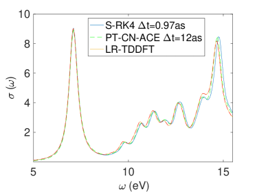
Figure 1: Partial absorption spectrum of benzene along the $x$ direction evaluated using the HSE06 functional.

In the second example, we study the response of a silicon system to an ultra-fast laser pulse. The supercell consists of 32 atoms, and is constructed from $2\times 2\times 1$ unit cells sampled at the $\Gamma$ point. Each simple cubic unit cell has $8$ silicon atoms, and the lattice constant is 5.43 Å . The kinetic energy cutoff is set to 10 Hartree. The laser is applied along the $x$ direction, and generates an electric field of the form

$$\textbf{E}(t)=\hat{\textbf{x}}E_{\text{max}}\exp\Big{[}-\frac{(t-t_{0})^{2}}{2a^{2}}\Big{]}\sin[\omega(t-t_{0})]{.}$$ (18)

Here $a=2.55$ fs, $\hbar\omega=3.26\mathrm{eV},t_{0}=15$ fs, which corresponds to a laser that peaks at $15$ fs with its wavelength being $380$ nm. The laser intensity $E_{\text{max}}$ is 0.0194 a.u. in the simulation. The profile of this external field is given in Fig. 2 (a). The ground state band gap computed at $t=0$ is around $1.0$ eV using the HSE06 functional with a supercell containing 64 atoms. The total simulation length is $29$ fs. In the PT-CN-ACE method, for the inner loop, the stopping criteria for the relative error of the electron density is set to $10^{-7}$. The stopping criteria for the outer loop is defined via the relative error of the Fock exchange energy, and is set to $10^{-8}$. The stopping criteria for the PT-CN method is defined via the relative error of the electron density and is set to $10^{-6}$. We remark that although this is a periodic system and electron polarization should be evaluated using e.g. theories based on localized Wannier functions ^{39, 40}, here for simplicity we just construct the laser field and measure the dipole moment by treating the silicon system as a large molecule. Such treatment is consistent among different choices of numerical measures, which is sufficient to demonstrate the efficiency and accuracy of the PT-CN-ACE algorithm.

In order to demonstrate the electron excitation process, we plot the density of states at the end of the simulation (Fig. 2 (b), the green dotted line indicates the Fermi energy), defined as

$$\rho(\varepsilon):=\sum_{j=1}^{N_{e}}\sum_{i=1}^{\infty}|\langle\psi_{i}(T)|\varphi_{j}(T)\rangle|^{2}\widetilde{\delta}(\varepsilon-\varepsilon_{i}(T)).$$

Here $\varphi_{j}(T)$ is the $j$-th orbital obtained at the end of the TDDFT simulation at time $T$, and $\varepsilon_{i}(T),\psi_{i}(T)$ are the eigenvalues and wavefunctions corresponding to the Hamiltonian at time $T$. $\widetilde{\delta}$ is a Dirac-$\delta$ function with a Gaussian broadening of $0.05$ eV.

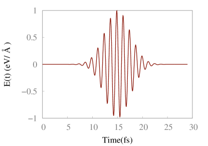
(a) Electric field along the $x$ direction

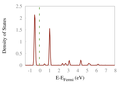
(b) Density of states at time $T$

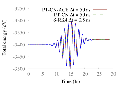
(c) Total energy

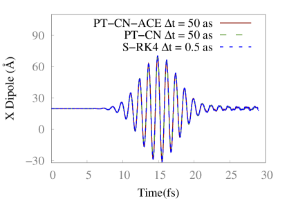
(d) Dipole moment along the $x$ direction

Figure 2: Electron dynamics of a 32 atom silicon system under a laser pulse.

Fig. 2 (c), (d) show the total energy and the dipole moment along the $x$ direction calculated with the PT-CN, PT-CN-ACE and S-RK4 methods. The time steps of both PT-CN and PT-CN-ACE are set to 50 as, while the time step of S-RK4 is set to 0.5 as due to stability reason. Both the energy and the dipole moment agree very well among the results obtained from these three methods, indicating that the use of the compressed exchange operator in PT-CN-ACE does not lead to any loss of accuracy. The total energy and dipole moment obtained from S-RK4 and PT-CN-ACE are nearly indistinguishable before $15$ fs, and becomes slightly different after 20 fs. Such error can be systematically reduced by using smaller time steps. Table 1 shows that the error can be reduced to as small as $0.016$ meV/atom when the time step is reduced to 2.4 as for PT-CN-ACE method. Nearly the same accuracy is also observed in the PT-CN method when reducing the time step. We also listed the speedup factors in terms of both the number of Fock exchange operator applications per orbital per time step (FOC) and the total wall clock time (Wtime) in Table 1. The Wtime speedup is denoted in “Speedup” in Table 1. In comparison, the Fock exchange operator application speedup, which is denoted as “Speedup*” in Table 1, is calculated by counting the number of Fock exchange operator application for a given time period $\Delta$t. Note that the speedup factor obtained from the number of Fock exchange operator applications is relatively bigger than the wall clock time speedup, especially for PT-CN-ACE. This is mainly because the inner loop calculation in PT-CN-ACE still takes a big proportion of the computational time for this relatively small system. It is also why PT-CN can be faster than PT-CN-ACE in terms of the wall clock time despite of the fact that PT-CN requires more Fock exchange operator applications per orbital. However, as the system size increases, the cost due to the Fock exchange operator becomes dominant, and we shall observe that PT-CN-ACE becomes more advantageous below.

Method	$\Delta t$(as)	AEI(meV)	AED(meV)	FOC	Speedup*	Wtime(h)	Speedup
S-RK4	0.5	621.4156	/	4.0	1.0	18.09	1.0
PT-CN	2.4	621.4062	0.009	4.8	4	6.0	3.0
PT-CN	5.1	621.4688	0.053	5.3	7.7	3.65	5
PT-CN	12.1	623.4656	2.05	5.9	16.4	1.45	12.4
PT-CN	25.0	628.8594	7.44	10.8	18.5	1.08	16.7
PT-CN	50.0	657.6688	36.25	21	19	1.12	16.1
PT-CN-ACE	2.4	621.4313	0.016	2.32	8.3	4.99	3.7
PT-CN-ACE	5.1	621.4937	0.08	2.77	14.7	3.11	5.8
PT-CN-ACE	12.1	623.5781	2.2	3.02	32.0	1.6	11.3
PT-CN-ACE	25.0	628.9531	7.5	3.78	52.9	1.45	12.5
PT-CN-ACE	50.0	657.725	36.3	5.8	69.0	1.38	13.1

Table 1: Accuracy and efficiency of PT-CN and PT-CN-ACE for the electron dynamics with the $380nm$ laser compared to S-RK4. The accuracy is measured using the average energy increase per atom (AEI) after $29.0$ fs and the average energy difference (AED) per atom for PT-CN and PT-CN-ACE compared with S-RK4 method after $29.0$fs. The efficiency is measured using the average number of Fock exchange operator applications per orbital in each time step (FOC) during the time interval from $0.0$ fs to $29.0$ fs, and the Fock exchange operator application speedup is denoted as “Speedup*”. The total wall clock time (Wtime) and the corresponding speedup factor are also listed.

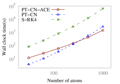
(a) Total wall clock time.

(b) Breakdown of the wall clock time, 1

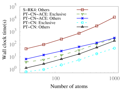
(c) Breakdown of the wall clock time, 2

Figure 3: Wall clock time for simulating silicon systems from 32 atoms up to 1024 atoms for $\Delta t=50$ as. The number of CPU cores used are set to $2\times N_{atom}$ in all tests. The systems are driven by the laser field shown at Fig. 2(a).

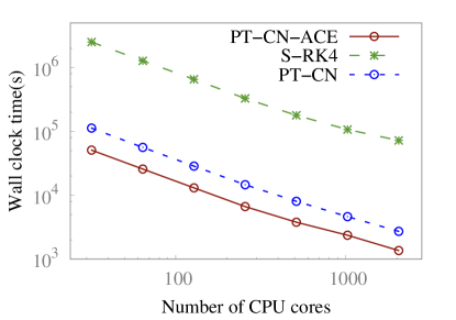
Figure 4: Total wall clock time for 1024 atom silicon system from 32 up to 2048 CPU cores used in $\Delta t=50$ as. The system is driven by laser field shown at Fig. 2(a).

Next we systematically investigate the efficiency of the PT-CN and PT-CN-ACE schemes by increasing the size of the supercell from $2\times 2\times 1$ to $8\times 4\times 4$ unit cells, and the set of systems consists of $32$ to $1024$ silicon atoms. All other physical parameters remain the same as in the tests above. We report the total wall clock time of the PT-CN, PT-CN-ACE and S-RK4 methods, as well as the breakdown into different components time of for a time period of $\Delta$t = 50 as. We report the performance in terms of both the weak scaling and the strong scaling. The time step of PT-CN and PT-CN-ACE is set to be 50 as and the time step for S-RK4 is $0.5$ as. The average number of Fock exchange operator applications per orbital for PT-CN and PT-CN-ACE is $21$ and $5.75$, respectively. For the PT-CN-ACE method, the average number of inner iterations is $24$.

The total wall clock time of PT-CN-ACE can be divided into four parts: “ACE operator”, which stands for the time used for applying the Fock exchange operator and constructing the ACE operator implicitly; “HPSI”, which represents the time for the $H\psi$ calculation, with the application of the exchange operator replaced by the application of the ACE operator via a matrix vector multiplication operation; “PT-CN-ACE: Exclusive”, which includes the time exclusively associated with the usage of the parallel transport gauge, such as the orbital mixing and orbital orthogonalization; and “Others”, which includes all other parts that are shared among the three methods, such as the evaluation of the Hartree potential and the total energy. Similarly, the total wall clock time of PT-CN is decomposed into three parts: “HPSI”, “PT-CN: Exclusive” and “Others”. The total wall clock time of S-RK4 is divided into “HPSI” and “Others”. Note that “HPSI” and the evaluation of the total energy in PT-CN and S-RK4 require the application of the true Fock exchange operator.

PWDFT is mainly parallelized along the orbital direction, i.e. the maximum number of cores is equal to the number of occupied orbitals. The application of the Fock exchange operator to the occupied orbitals is implemented using the fast Fourier transformation(FFT). In the “HPSI” component of the PT-CN-ACE method, the matrix matrix multiplication between the low rank operator $\widetilde{V}_{\mathrm{X}}$ and all the occupied orbitals is performed to evaluate the Fock exchange term. We remark that certain components of PWDFT, such as the solution of the Hartree potential, are currently carried out on a single core. This is consistent with the choice of parallelization along the orbital direction, where each $H\psi$ (except the application of the Fock exchange operator) is carried out on a single core. However, as will be shown below, PT-CN-ACE and S-RK4 typically requires many more Hartree potential evaluation compared to PT-CN. Hence PT-CN has some advantage in terms of the wall clock time from this perspective.

Fig. 3 (a) shows the total wall clock time with respect to the system size $N_{atom}$ for all three method. In these tests the number of CPU cores used is always proportional to the number of atoms, i.e. $2\times N_{atom}$ (this is called “weak scaling”). The speedup of PT-CN-ACE over S-RK4 is 7 times at 32 atoms, and increases to 46 times at 1024 atoms. On the other hand, the speedup of PT-CN over S-RK4 is between 22 and 23 times, which is consistent with the Fock exchange operator applications speedup as shown in Table 1. For small systems, PT-CN is the most efficient method. When the system size increases beyond 256 atoms, PT-CN-ACE becomes the most efficient one in terms of the wall clock time. This cross-over can be explained by the breakdown of the total time shown in Fig. 3 (b) (c). Since PT-CN-ACE method introduces a nested loop to reduce the number of Fock exchange operator applications, it also increases the number of inner iterations. More specifically, in the tests above, the number of Fock exchange operator applications per orbital is $6$, but the number of inner iterations is $120$ in PT-CN-ACE. In comparison, PT-CN only requires $21$ inner iterations. Thus PT-CN is faster than PT-CN-ACE at small system size as shown in Fig.  3(a). However, as system size becomes larger, the Fock exchange operator applications will dominate the cost, and PT-CN-ACE becomes faster than PT-CN as shown in Fig. 3(a).

More specifically, Fig. 3(b) shows that “HPSI” takes 49 to 78 percent of total wall clock time from 32 to 1024 atom system for the S-RK4 method. For the PT-CN method, “HPSI” costs 51 percent of the time for the system with 32 atoms, and this becomes 91 percent when the system size increases to 1024 atoms. For the PT-CN-ACE method, the cost involving the Fock exchange operator is reduced to only 4 percent of the total time for the system with 32 atoms, and becomes 53 percent for the system with 1024 atoms.

Finally we report in Fig. 4 the average wall clock time for carrying out a simulation of $50$ as for the 1024 atom silicon system, with respect to the increase of the number of computational cores (this is called “strong scaling”). Compared to performance using 32 cores, the parallel efficiency of a single TDDFT step with 2048 cores reaches 54 percent, 58 percent and 64 percent for the S-RK4, PT-CN-ACE and PT-CN methods, respectively. The reduction of the parallel efficiency is mainly caused by our sequential implementation of certain components, such as the evaluation of the Hartree potential. The speedup of PT-CN-ACE method over S-RK4 is between 46 times and 50 times over the entire range. Therefore in order to finish the electron dynamics simulation above of $29$ fs, it will take about 1 year using S-RK4, and this is reduced to around one week using PT-CN-ACE. Such a simulation is by all means still expensive, but starts to become feasible to be routinely performed.

6 Conclusion

In order to accelerate large scale hybrid functional rt-TDDFT calculations, we have presented a method to combine two recently developed ideas: parallel transport (PT) gauge and adaptively compressed exchange (ACE) operator. The overall goal is to reduce the frequency for the application of the Fock exchange operator to orbitals, with systematically controlled accuracy. We demonstrate that the resulting PT-CN-ACE scheme can indeed reduce the number of Fock exchange operator applications per unit time by one to two orders of magnitude compared to the standard explicit 4th order Runge-Kutta time integrator, and thus enables hybrid functional rt-TDDFT calculations for systems up to $1000$ atoms for the first time.

Compared to the PT-CN scheme, the extra reduction of the number of applications of the Fock exchange operator requires more iterations in the inner loop. This is consistent with the observation for ground state hybrid functional calculations ⁴¹. Hence in our implementation, PT-CN is in fact faster than PT-CN-ACE in terms of wall clock time for small systems. The precise cross-over point depends heavily on the cost for solving the Poisson-like equation to apply the Fock exchange operator. For instance, we expect that the PT-CN-ACE becomes advantageous at a much earlier stage in real space rt-TDDFT software packages, where the solution of a Poisson-like equation can be much more expensive than that in a planewave based code. On the other hand, if the application of the Fock exchange operator can be accelerated using techniques such as localization ^{42, 43}, density fitting ^{44, 45, 46}, or through the GPU architecture, we expect that the original PT-CN scheme will be more favorable. Further developments to reduce the number of inner iterations without penalizing the number of Fock exchange operator applications, such as via the usage of better preconditioners, is also an interesting direction for future works.

7 Acknowledgments

This work was partially supported by the National Science Foundation under Grant No. 1450372, No. DMS-1652330 (W. J. and L. L.), and by the Department of Energy under Grant No. DE-SC0017867, No. DE-AC02-05CH11231 (L. L.). We thank the National Energy Research Scientific Computing (NERSC) center and the Berkeley Research Computing (BRC) program at the University of California, Berkeley for making computational resources available. We thank Dong An, Zhanghui Chen and Lin-Wang Wang for helpful discussions.

References

- Hohenberg and Kohn 1964 Hohenberg, P.; Kohn, W. Inhomogeneous electron gas. Phys. Rev. 1964, 136, B864–B871
- Kohn and Sham 1965 Kohn, W.; Sham, L. Self-consistent equations including exchange and correlation effects. Phys. Rev. 1965, 140, A1133–A1138
- Lee et al. 1988 Lee, C.; Yang, W.; Parr, R. G. Development of the Colle-Salvetti correlation-energy formula into a functional of the electron density. Phys. Rev. B 1988, 37, 785–789
- Becke 1993 Becke, A. D. Density functional thermochemistry. III. The role of exact exchange. J. Chem. Phys. 1993, 98, 5648
- Perdew et al. 1996 Perdew, J. P.; Ernzerhof, M.; Burke, K. Rationale for mixing exact exchange with density functional approximations. J. Chem. Phys. 1996, 105, 9982–9985
- Heyd et al. 2003 Heyd, J.; Scuseria, G. E.; Ernzerhof, M. Hybrid functionals based on a screened Coulomb potential. J. Chem. Phys. 2003, 118, 8207–8215
- Heyd et al. 2006 Heyd, J.; Scuseria, G. E.; Ernzerhof, M. Erratum:“Hybrid functionals based on a screened Coulomb potential”[J. Chem. Phys. 118, 8207 (2003)]. J. Chem. Phys. 2006, 124, 219906
- Stroppa and Kresse 2008 Stroppa, A.; Kresse, G. The shortcomings of semi-local and hybrid functionals: what we can learn from surface science studies. New Journal of Physics 2008, 10, 063020
- Marsman et al. 2008 Marsman, M.; Paier, J.; Stroppa, A.; Kresse, G. Hybrid functionals applied to extended systems. Journal of Physics: Condensed Matter 2008, 20, 064201
- Takimoto et al. 2007 Takimoto, Y.; Vila, F. D.; Rehr, J. J. Real-time time-dependent density functional theory approach for frequency-dependent nonlinear optical response in photonic molecules. J. Chem. Phys. 2007, 127, 154114
- Krasheninnikov et al. 2007 Krasheninnikov, A. V.; Miyamoto, Y.; Tománek, D. Role of electronic excitations in ion collisions with carbon nanostructures. Phys. Rev. Lett. 2007, 99, 016104
- Runge and Gross 1984 Runge, E.; Gross, E. K. U. Density-functional theory for time-dependent systems. Phys. Rev. Lett. 1984, 52, 997
- Yabana and Bertsch 1996 Yabana, K.; Bertsch, G. F. Time-dependent local-density approximation in real time. Phys. Rev. B 1996, 54, 4484–4487
- Onida et al. 2002 Onida, G.; Reining, L.; Rubio, A. Electronic excitations: density-functional versus many-body Green’s-function approaches. Rev. Mod. Phys. 2002, 74, 601
- Andreani et al. 2005 Andreani, C.; Colognesi, D.; Mayers, J.; Reiter, G.; Senesi, R. Measurement of momentum distribution of light atoms and molecules in condensed matter systems using inelastic neutron scattering. Adv. Phys. 2005, 54, 377–469
- Alonso et al. 2008 Alonso, J. L.; Andrade, X.; Echenique, P.; Falceto, F.; Prada-Gracia, D.; Rubio, A. Efficient formalism for large-scale ab initio molecular dynamics based on time-dependent density functional theory. Phys. Rev. Lett. 2008, 101, 096403
- Ullrich 2011 Ullrich, C. A. Time-dependent density-functional theory: concepts and applications; Oxford Univ. Pr., 2011
- Lopata and Govind 2011 Lopata, K.; Govind, N. Modeling fast electron dynamics with real-time time-dependent density functional theory: Application to small molecules and chromophores. J. Chem. Theory Comput. 2011, 7, 1344–1355
- Lopata et al. 2012 Lopata, K.; Van Kuiken, B. E.; Khalil, M.; Govind, N. Linear-Response and Real-Time Time-Dependent Density Functional Theory Studies of Core-Level Near-Edge X-Ray Absorption. J. Chem. Theory Comput. 2012, 8, 3284–3292
- Ding et al. 2013 Ding, F.; Van Kuiken, B. E.; Eichinger, B. E.; Li, X. An efficient method for calculating dynamical hyperpolarizabilities using real-time time-dependent density functional theory. J. Chem. Phys. 2013, 138, 064104
- Castro et al. 2004 Castro, A.; Marques, M.; Rubio, A. Propagators for the time-dependent Kohn-Sham equations. J. Chem. Phys. 2004, 121, 3425–33
- Schleife et al. 2012 Schleife, A.; Draeger, E. W.; Kanai, Y.; Correa, A. A. Plane-wave pseudopotential implementation of explicit integrators for time-dependent Kohn-Sham equations in large-scale simulations. J. Chem. Phys. 2012, 137, 22A546
- Gómez Pueyo et al. 2018 Gómez Pueyo, A.; Marques, M. A.; Rubio, A.; Castro, A. Propagators for the time-dependent Kohn-Sham equations: multistep, Runge-Kutta, exponential Runge-Kutta, and commutator free Magnus methods. J. Chem. Theory. Comput. 2018,
- 24 An, D.; Lin, L. Quantum dynamics with the parallel transport gauge. arXiv:1804.02095
- 25 Jia, W.; An, D.; Wang, L.-W.; Lin, L. Fast real-time time-dependent density functional theory calculations with the parallel transport gauge. arXiv:1805.10575
- Lin 2016 Lin, L. Adaptively Compressed Exchange Operator. J. Chem. Theory Comput. 2016, 12, 2242
- Hu et al. 2017 Hu, W.; Lin, L.; Banerjee, A.; Vecharynski, E.; Yang, C. Adaptively compressed exchange operator for large scale hybrid density functional calculations with applications to the adsorption of water on silicene. submitted 2017,
- Giannozzi et al. 2009 Giannozzi, P.; Baroni, S.; Bonini, N.; Calandra, M.; Car, R.; Cavazzoni, C.; Ceresoli, D.; Chiarotti, G. L.; Cococcioni, M.; Dabo, I.; Corso, A. D.; de Gironcoli, S.; Fabris, S.; Fratesi, G.; Gebauer, R.; Gerstmann, U.; Gougoussis, C.; Kokalj, A.; Lazzeri, M.; Martin-Samos, L.; Marzari, N.; Mauri, F.; Mazzarello, R.; Paolini, S.; Pasquarello, A.; Paulatto, L.; Sbraccia, C.; Scandolo, S.; Sclauzero, G.; Seitsonen, A. P.; Smogunov, A.; Umari, P.; Wentzcovitch, R. M. QUANTUM ESPRESSO: a modular and open-source software project for quantum simulations of materials. J. Phys.: Condens. Matter 2009, 21, 395502–395520
- Lin and Lindsey 2017 Lin, L.; Lindsey, M. Convergence of adaptive compression methods for Hartree-Fock-like equations. arXiv:1703.05441 2017,
- Lin et al. 2017 Lin, L.; Xu, Z.; Ying, L. Adaptively Compressed Polarizability Operator for Accelerating Large Scale Ab Initio Phonon Calculations. Multiscale Model. Simul. 2017, 15, 29–55
- Anderson 1965 Anderson, D. G. Iterative procedures for nonlinear integral equations. J. Assoc. Comput. Mach. 1965, 12, 547–560
- Andrade et al. 2012 Andrade, X.; Alberdi-Rodriguez, J.; Strubbe, D. A.; Oliveira, M. J. T.; Nogueira, F.; Castro, A.; Muguerza, J.; Arruabarrena, A.; Louie, S. G.; Aspuru-Guzik, A.; Rubio, A.; Marques, M. A. L. Time-dependent density-functional theory in massively parallel computer architectures: the octopus project. J. Phys. Condens. Matter 2012, 24, 233202
- Jornet-Somoza et al. 2015 Jornet-Somoza, J.; Alberdi-Rodriguez, J.; Milne, B. F.; Andrade, X.; Marques, M.; Nogueira, F.; Oliveira, M.; Stewart, J.; Rubio, A. Insights into colour-tuning of chlorophyll optical response in green plants. Phys. Chem. Chem. Phys. 2015, 17, 26599–26606
- Lin et al. 2012 Lin, L.; Lu, J.; Ying, L.; E, W. Adaptive local basis set for Kohn-Sham density functional theory in a discontinuous Galerkin framework I: Total energy calculation. J. Comput. Phys. 2012, 231, 2140–2154
- Hu et al. 2015 Hu, W.; Lin, L.; Yang, C. DGDFT: A massively parallel method for large scale density functional theory calculations. J. Chem. Phys. 2015, 143, 124110
- Hamann 2013 Hamann, D. R. Optimized norm-conserving Vanderbilt pseudopotentials. Phys. Rev. B 2013, 88, 085117
- Schlipf and Gygi 2015 Schlipf, M.; Gygi, F. Optimization algorithm for the generation of ONCV pseudopotentials. Comput. Phys. Commun. 2015, 196, 36–44
- Malcıoğlu et al. 2011 Malcıoğlu, O. B.; Gebauer, R.; Rocca, D.; Baroni, S. turboTDDFT–A code for the simulation of molecular spectra using the Liouville–Lanczos approach to time-dependent density-functional perturbation theory. Comput. Phys. Commun. 2011, 182, 1744–1754
- King-Smith and Vanderbilt 1993 King-Smith, R. D.; Vanderbilt, D. Theory of polarization of crystalline solids. Phys. Rev. B 1993, 47, 1651
- Marzari et al. 2012 Marzari, N.; Mostofi, A. A.; Yates, J. R.; Souza, I.; Vanderbilt, D. Maximally localized Wannier functions: Theory and applications. Rev. Mod. Phys. 2012, 84, 1419–1475
- Hu et al. 2017 Hu, W.; Lin, L.; Yang, C. Projected Commutator DIIS Method for Accelerating Hybrid Functional Electronic Structure Calculations. J. Chem. Theory Comput. 2017, 13, 5458
- Marzari and Vanderbilt 1997 Marzari, N.; Vanderbilt, D. Maximally localized generalized Wannier functions for composite energy bands. Phys. Rev. B 1997, 56, 12847
- Damle et al. 2015 Damle, A.; Lin, L.; Ying, L. Compressed Representation of Kohn–Sham Orbitals via Selected Columns of the Density Matrix. J. Chem. Theory Comput. 2015, 11, 1463–1469
- Lu and Ying 2015 Lu, J.; Ying, L. Compression of the electron repulsion integral tensor in tensor hypercontraction format with cubic scaling cost. J. Comput. Phys. 2015, 302, 329
- Hu et al. 2017 Hu, W.; Lin, L.; Yang, C. Interpolative separable density fitting decomposition for accelerating hybrid density functional calculations with applications to defects in silicon. J. Chem. Theory Comput. 2017, 13, 5420
- Dong et al. 2018 Dong, K.; Hu, W.; Lin, L. Interpolative separable density fitting through centroidal Voronoi tessellation with applications to hybrid functional electronic structure calculations. J. Chem. Theory Comput. in press 2018,