The $\text{T}\bar{\text{T}}$ perturbation and its geometric interpretation

Abstract

Starting from the recently-discovered $\text{T}\bar{\text{T}}$-perturbed Lagrangians, we prove that the deformed solutions to the classical EoMs for bosonic field theories are equivalent to the unperturbed ones but for a specific field-dependent local change of coordinates. This surprising geometric outcome is fully consistent with the identification of $\text{T}\bar{\text{T}}$-deformed 2D quantum field theories as topological JT gravity coupled to generic matter fields. Although our conclusion is valid for generic interacting potentials, it first emerged from a detailed study of the sine-Gordon model and in particular from the fact that solitonic pseudo-spherical surfaces embedded in $\mathbb{R}^{3}$ are left invariant by the deformation. Analytic and numerical results concerning the perturbation of specific sine-Gordon soliton solutions are presented.

1 Introduction

The deformation of 2D quantum field theories Smirnov:2016lqw ; Cavaglia:2016oda by the Zamolodchikov’s $\text{T}\bar{\text{T}}$ operator Zamolodchikov:2004ce , has recently attracted the attention of theoretical physicists due to the many important links with string theory Dubovsky:2012wk ; dubovsky2012effective ; Caselle:2013dra ; Chen:2018keo and AdS/CFT McGough:2016lol ; Turiaci:2017zwd ; Giveon:2017nie ; Giveon:2017myj ; Asrat:2017tzd ; Giribet:2017imm ; Kraus:2018xrn ; Cottrell:2018skz ; Baggio:2018gct ; Babaro:2018cmq .

A remarkable property of this perturbation, discovered in Smirnov:2016lqw ; Cavaglia:2016oda , concerns the evolution of the quantum spectrum at finite volume $R$, with periodic boundary conditions, in terms of the $\text{T}\bar{\text{T}}$ coupling constant $\tau$. The spectrum is governed by the inhomogeneous Burgers equation

$$\partial_{\tau}E_{n}(R,\tau)=\frac{1}{2}\partial_{R}\left(E_{n}^{2}(R,\tau)-P_{n}^{2}(R)\right)\;,$$ (1)

where $E_{n}(R,\tau)$ and $P_{n}(R)$ are the total energy and momentum of a generic energy eigenstate $|n\rangle$, respectively. Equation (1) is valid also for non-integrable models.

Notice that (1) reveals an important feature of $\text{T}\bar{\text{T}}$-deformed QFTs: the interaction between the perturbing operator and the geometry, through the coupling $\tau$. The latter property is a basic requirement for any sensible theory of gravity but in the current case it naturally emerges, non perturbatively and at full quantum level, from a specific irrelevant perturbation of Lorentz-invariant Quantum Field Theories (QFTs). An important link with JT topological gravity was noticed and studied in Dubovsky:2017cnj , where it was shown that JT gravity coupled to matter leads to a scattering phase matching that associated to the $\text{T}\bar{\text{T}}$ perturbation Mussardo:1999aj ; Zamolodchikov:1991vx ; Dubovsky:2012wk ; dubovsky2012effective ; Caselle:2013dra ; Dubovsky:2013ira ; Smirnov:2016lqw ; Cavaglia:2016oda .

Studies of partition functions Cavaglia:2016oda ; Cardy:2018sdv ; Dubovsky:2018bmo ; Datta:2018thy have led to a proof of the uniqueness of this perturbation Aharony:2018bad under the assumption that the theory on the torus is invariant under modular transformations and that the energy of a given eigenstate is a function only of $\tau$ and of the energy and momentum of the corresponding state at $\tau=0$. Furthermore, starting from the JT-gravity setup, in Dubovsky:2018bmo the hydrodynamic-type equation (1) was recovered. The latter result together with Dubovsky:2017cnj confirms, beyond any reasonable doubt, the equivalence between the $\text{T}\bar{\text{T}}$ deformation and JT topological gravity coupled to generic matter field.

The aim of this paper is to address the problem concerning the classical interpretation of the $\text{T}\bar{\text{T}}$ perturbation following the more direct approach proposed in Cavaglia:2016oda and further developed in Bonelli:2018kik ; Conti:2018jho . The current analysis is based on the observation Smirnov:2016lqw ; Cavaglia:2016oda that (1) directly implies a self-consistent flow equation for the deformed Lagrangian $\mathcal{L}^{(\tau)}$

$$\partial_{\tau}\mathcal{L}^{(\tau)}=\textrm{Det}\left(T^{(\tau)}_{\mu\nu}\right)\;,\quad T^{(\tau)}_{\mu\nu}=-{\textstyle\frac{2}{\sqrt{|g|}}}{\textstyle\frac{\delta(\mathcal{L}^{(\tau)}\sqrt{|g|})}{\delta g^{\mu\nu}}}\;,$$ (2)

where $g=\textrm{Det}\left(g_{\mu\nu}\right)$ and $\text{T}\bar{\text{T}}=-\pi^{2}\textrm{Det}\left(T_{\mu\nu}\right)$ is the classical counterpart of Zamolodchikov’s operator.

Starting from the unperturbed Lagrangian $\mathcal{L}^{(0)}$ equation (2) can be solved giving the $\text{T}\bar{\text{T}}$-deformed exact result $\mathcal{L}^{(\tau)}$. Adopting this strategy, the Nambu-Goto classical Lagrangian in the static gauge was recovered Cavaglia:2016oda along with the deformation of bosonic models with generic interacting potential Cavaglia:2016oda ; Bonelli:2018kik ; Conti:2018jho , WZW and $\sigma$-models Baggio:2018gct ; Bonelli:2018kik ; Dei:2018mfl , and the Thirring model Bonelli:2018kik .

There are many reasons to study these newly-discovered set of classical Lagrangians. First of all, according to Dubovsky:2017cnj ; Dubovsky:2018bmo , these systems should correspond to JT gravity coupled to non-topological matter, a fact that is by no mean evident from the Lagrangian point of view.

Secondly, when the starting model is integrable, there should be a general way to deform the whole integrable model machinery. For example, a generalisation of the ODE/IM correspondence Dorey:1998pt ; Bazhanov:1998wj ; Dorey:2007zx should lead to an alternative method to obtain the quantum spectrum at finite volume Lukyanov:2010rn ; Dorey:2012bx and it may open the way to the inclusion of the $\text{T}\bar{\text{T}}$ inside the Wilson Loops/Scattering Amplitudes setup, in $\text{AdS}_{5}/\text{CFT}_{4}$ Alday:2009dv ; Alday:2010vh and perhaps also to consistently deform the Argyres-Douglas theory Gaiotto:2014bza ; Ito:2017ypt ; Grassi:2018bci .

The main purpose of this article is to prove that, for bosonic theories with arbitrary interacting potentials, the $\text{T}\bar{\text{T}}$ perturbation has indeed the alternative interpretation as a space-time deformation. In Euclidean coordinates the change of variables is

$$dx^{\mu} = \left(\delta^{\mu}_{\;\;\nu}+\tau\widetilde{T}^{\mu}_{\;\;\nu}(\mathbf{y})\right)dy^{\nu}\;,\quad\mathbf{y}=(y^{1},y^{2})\;,$$ (3)

$$dy^{\mu} = \left(\delta^{\mu}_{\;\;\nu}+\tau\bigl{(}\widetilde{T}^{(\tau)}\bigr{)}^{\mu}_{\;\;\nu}(\mathbf{x})\right)dx^{\nu}\;,\quad\mathbf{x}=(x^{1},x^{2})\;,$$ (4)

with $\widetilde{T}^{\mu}_{\;\;\nu}=-\epsilon^{\mu}_{\;\;\rho}\epsilon^{\sigma}_{\;\;\nu}T^{\rho}_{\;\;\sigma}$ and $\bigl{(}\widetilde{T}^{(\tau)}\bigr{)}^{\mu}_{\;\;\nu}=-\epsilon^{\mu}_{\;\;\rho}\epsilon^{\sigma}_{\;\;\nu}\bigl{(}T^{(\tau)}\bigr{)}^{\rho}_{\;\;\sigma}$, where $T=T^{(0)}$ and $T^{(\tau)}$ are the unperturbed and perturbed stress-energy tensor in the set of coordinates $\mathbf{y}$ and $\mathbf{x}$, respectively. Then, any solution of the perturbed EoMs can be mapped onto the $\tau=0$ corresponding solution, i.e.

$$\phi^{(\tau)}(\mathbf{x})=\phi^{(0)}\left(\mathbf{y}(\mathbf{x})\right)\;,$$ (5)

where the r.h.s. of (5) is defined on a deformed space-time with metric

$${\bf g}^{\prime}_{\mu\nu}=\delta_{\mu\nu}-\tau\epsilon_{\mu\rho}\epsilon^{\sigma}_{\;\;\nu}\left(2T+\tau T^{2}\right)^{\rho}_{\;\;\sigma}\;.$$ (7)

In fact (4) corresponds to a natural generalization of the Virasoro conditions used in the GGRT treatment of the NG string Goddard:1973qh , and it matches precisely the generalisation corresponding to classical JT gravity Dubovsky:2017cnj ; Dubovsky:2018bmo .

2 Classical integrable equations and embedded surfaces

It is an established fact that integrable equations in two dimensions admit an interpretation in terms of surfaces embedded inside an $N$-dimensional space. The two oldest examples of this connection, dating back to the works of 19th century geometers Bour_862 ; Liou_853 , are the sine-Gordon and Liouville equations. They appear as the Gauss-Mainardi-Codazzi (GMC) system of equations (139) for, respectively, pseudo-spherical and minimal surfaces embedded in the Euclidean space $\mathbb{R}^{3}$. As proved by Bonnet Bonn_867 , any surface embedded in $\mathbb{R}^{3}$ is uniquely determined (up to its position in the ambient space) by two rank $2$ symmetric tensors: the metric $g_{\mu\nu}$ (129) and the second fundamental tensor $d_{\mu\nu}$ (131). Their intuitive role is to measure, respectively, the length of an infinitesimal curve and the displacement of its endpoint from the tangent plane at the starting point. One can then use $g_{\mu\nu}$ and $d_{\mu\nu}$ to study the motion of a frame anchored to the surface. The result is a system of linear differential equations, known as Gauss-Weingarten equations (134, 135). The GMC system appears then as the consistency condition for this linear system, effectively constraining the “moduli space” consisting of the two tensors $g_{\mu\nu}$ and $d_{\mu\nu}$.

The search for a general correspondence originated in the works of Lund, Regge, Pohlmeyer and Getmanov Pohl_76 ; Lund_Regg_76 ; Getm_77 and was subsequently formalised by Sym Sym_82 ; Sym_83 ; Sym_84_1 ; Sym_84_2 ; Sym_84_3 who showed that any integrable system whose associated linear problem is based on a semi-simple Lie algebra $\mathfrak{g}$ can be put in the form of a GMC system for a surface embedded in a $\textrm{dim}(\mathfrak{g})$-dimensional surface. In this section we will shortly review Sym’s results for the general setting and concentrate on the case of sine-Gordon model. We will use the following conventions

$$\mathbf{z}=\left(z^{1},z^{2}\right)\;,\quad\partial_{\mu}f\left(\mathbf{z}\right)\equiv\frac{\partial}{\partial z^{\mu}}f\left(\mathbf{z}\right)\;,\quad\forall f\;:\;\mathbb{R}^{2}\;\rightarrow\mathbb{R}\;,\quad\mu=1,2\;.$$

2.1 Construction of the solitonic surfaces

Let us consider a generic $2$-dimensional system of non-linear partial differential equations for a set of real fields $\left\{\phi_{i}\left(\mathbf{z}\right)\right\}$ admitting a Zero Curvature Representation (ZCR) for a pair of functions $L_{1}$ and $L_{2}$ taking values in a $d$-dimensional representation of a semi-simple Lie algebra $\mathfrak{g}$ ($\textrm{dim}(\mathfrak{g})=N$):

$$\partial_{2}L_{1}-\partial_{1}L_{2}+\left[L_{1},L_{2}\right]=0\;.$$ (8)

The functions $L_{\mu}$ depend on $\mathbf{z}$ through the fields $\phi_{i}\left(\mathbf{z}\right)$ and their derivatives and on a real spectral parameter $\lambda$:

$$L_{\mu}\equiv L_{\mu}\left(\mathbf{z}|\lambda\right)\equiv L_{\mu}\left(\left\{\phi_{i}\left(\mathbf{z}\right)\right\},\left\{\partial_{\nu}\phi_{i}\left(\mathbf{z}\right)\right\},\ldots|\lambda\right)\;.$$ (9)

The Zero Curvature Representation can be interpreted as the compatibility condition for a system of first-order linear partial differential equations involving an auxiliary $d\times d$ matrix-valued function $\Phi\equiv\Phi\left(\mathbf{z}|\lambda\right)$

$$\partial_{\mu}\Phi=L_{\mu}\Phi\;,\quad\mu=1,2\;,$$ (10)

commonly known as associated linear problem. Assuming $\Phi\left(\mathbf{z}_{0}|\lambda\right)\in G$ as initial condition, with $G$ being the Lie group associated to $\mathfrak{g}$, equation (10) allows, in principle, to recover a single-valued function $\Phi\in G$ in the whole $\mathbb{R}^{2}$. This function can then be used to construct the following object

$$r\left(\mathbf{z}|\lambda\right)=\Phi^{-1}\left(\mathbf{z}|\lambda\right)\frac{\partial}{\partial\lambda}\Phi\left(\mathbf{z}|\lambda\right)\;,$$ (11)

which is interpreted as the coordinate description of a $\lambda$-family of surfaces embedded into the $N$-dimensional affine space $\mathfrak{g}$. Moreover, equipping the affine space $\mathfrak{g}$ with a non-degenerate scalar product (i.e. the Killing form of the semi-simple Lie algebra), we can convert $\mathfrak{g}$ into an $N$-dimensional flat space. In other words, we can find an orthonormal basis $\left\{\mathbf{e}^{i}\right\}$ of $\mathfrak{g}$ with respect to the Killing form and then extract the quantities $r_{i}$ from the identity

$$r=\sum_{i=1}^{N}r_{i}\mathbf{e}^{i}=\Phi^{-1}\left(\mathbf{z}|\lambda\right)\frac{\partial}{\partial\lambda}\Phi\left(\mathbf{z}|\lambda\right)\;.$$ (12)

The vector $\mathbf{r}=\left(\begin{array}[]{c c c c}r_{1},r_{2},\ldots,r_{N}\end{array}\right)^{T}$ is then the position vector of a family of surfaces embedded in $N$-dimensional flat space, parametrised by $\lambda$. These are called solitonic surfaces and satisfy the following properties:

1. their GMC system reduces to the ZCR (8). This means that any integrable system whose EoMs can be represented as a ZCR depending on a spectral parameter $\lambda$, can be associated to a particular class of surfaces;

2. they are invariant with respect to $\lambda$-independent gauge transformation of the pair $L_{\mu}$. This fact provides a way to prove the equivalence of distinct soliton systems up to gauge transformations and independent coordinate redefinitions, see Sym_84_2 ;

3. their metric tensor (induced by the flat space $\mathfrak{g}$) is explicitly computed from the pair $L_{\mu}$ as

   $$g_{\mu\nu}=\textrm{Tr}\left(\textrm{\bf Ad}\left(\frac{\partial L_{\mu}}{\partial\lambda}\right)\textrm{\bf Ad}\left(\frac{\partial L_{\nu}}{\partial\lambda}\right)\right)\;,$$ (13)

   where Ad denotes the adjoint representation of the algebra $\mathfrak{g}$. Consequently, any intrinsic property of the soliton surface is determined uniquely by the ZCR.

2.2 The case of sine-Gordon

Let us now consider the specific case of the sine-Gordon equation

$$\partial\bar{\partial}\phi=\frac{m^{2}}{\beta}\sin\left(\beta\phi\right)\;,$$ (14)

where we set $\mathbf{z}=(z^{1},z^{2})=(z,\bar{z})$. The ZCR for this model is well known

$$L_{1}^{\textrm{sG}}=\mathcal{Z}=\frac{\beta}{2}\partial\phi\;\mathcal{S}^{3}+\mathbbm{i}m\lambda\left[\cos\left(\frac{\beta}{2}\phi\right)\mathcal{S}^{1}-\sin\left(\frac{\beta}{2}\phi\right)\mathcal{S}^{2}\right]\;,$$ (15)

$$L_{2}^{\textrm{sG}}=\bar{\mathcal{Z}}=-\frac{\beta}{2}\bar{\partial}\phi\;\mathcal{S}^{3}+\mathbbm{i}\frac{m}{\lambda}\left[\cos\left(\frac{\beta}{2}\phi\right)\mathcal{S}^{1}+\sin\left(\frac{\beta}{2}\phi\right)\mathcal{S}^{2}\right]\;,$$ (16)

where $\mathcal{S}^{j}$ are the generators of $\mathfrak{su}\left(2\right)$

$$\left[\mathcal{S}^{i},\mathcal{S}^{j}\right]=\varepsilon^{ij}_{\phantom{ij}k}\;\mathcal{S}^{k}\;.$$ (17)

Since $\textrm{dim}\left(\mathfrak{su}\left(2\right)\right)=3$, we know that we are dealing with a surface embedded in the Euclidean plane $\mathbb{R}^{3}$ ($\mathfrak{su}\left(2\right)$ is compact). As mentioned in section 2, Bonnet theorem Bonn_867 tells us that any surface in $\mathbb{R}^{3}$ is completely specified (modulo its position) by its first and second fundamental quadratic forms, which can be computed easily:

$$\textsc{I}^{\textrm{sG}} =g^{\textrm{sG}}_{\mu\nu}dz^{\mu}dz^{\nu}=2m^{2}\left[\left(dz\right)^{2}-\frac{2}{\lambda^{2}}\cos\left(\beta\phi\right)dzd\bar{z}+\frac{1}{\lambda^{4}}\left(d\bar{z}\right)^{2}\right]\;,$$ (18)

$$\textsc{II}^{\textrm{sG}} =d^{\textrm{sG}}_{\mu\nu}dz^{\mu}dz^{\nu}=2m^{2}\frac{\sqrt{2}}{\lambda}\sin\left(\beta\phi\right)dzd\bar{z}\;.$$ (19)

From (18) and 19) one can then extract the Gaussian and the mean curvatures using (133):

$$K^{\textrm{sG}}=\textrm{Det}\left(d^{\textrm{sG}}_{\mu\rho}\,\left(g^{\textrm{sG}}\right)^{\rho\nu}\right)=-\frac{\lambda^{2}}{2}\;,\quad H^{\textrm{sG}}=d^{\textrm{sG}}_{\mu\nu}\,\left(g^{\textrm{sG}}\right)^{\nu\mu}=\frac{\lambda}{\sqrt{2}}\cot\left(\beta\phi\right)\;,$$ (20)

with $g^{\textrm{sG}}_{\mu\nu}\left(g^{\textrm{sG}}\right)^{\nu\rho}=\delta_{\mu}^{\rho}$. The fact that $K^{\textrm{sG}}$ is constant negative tells us that we are dealing with a pseudo-spherical surface, which we were expecting from the old results of Bour Bour_862 . Thus, for this specific case, the solitonic surfaces correspond to pseudo-spherical ones, with the spectral parameter $\lambda$ playing the role of Gaussian curvature.

3 The $\text{T}\bar{\text{T}}$-deformed sine-Gordon model and its associated surfaces

Let us now apply the Sym formalism sketched above to the $\text{T}\bar{\text{T}}$-deformed sine-Gordon model Conti:2018jho

$$\partial\left(\frac{\bar{\partial}\phi}{S}\right)+\bar{\partial}\left(\frac{\partial\phi}{S}\right)=\frac{V^{\prime}}{4S}\left(\frac{S+1}{1-\tau V}\right)^{2}\;,$$ (21)

$$S=\sqrt{1+4\tau\left(1-\tau V\right)\partial\phi\bar{\partial}\phi}\;,$$ (22)

$$V=2\frac{m^{2}}{\beta^{2}}\left(1-\cos(\beta\phi)\right)\;,\quad V^{\prime}=2\frac{m^{2}}{\beta}\sin(\beta\phi)\;,$$ (23)

and derive the geometric properties of the associated surfaces. We start with the ZCR, which was found in Conti:2018jho

$$L_{1}^{\text{T}\bar{\text{T}}} \equiv\mathcal{Z}=\beta\frac{\partial\phi}{2S}\;\mathcal{S}^{3}+2\mathbbm{i}m\left[F_{+}\cos\left(\frac{\beta}{2}\phi\right)\mathcal{S}^{1}-F_{-}\sin\left(\frac{\beta}{2}\phi\right)\mathcal{S}^{2}\right]\;,$$ (24)

$$L_{2}^{\text{T}\bar{\text{T}}} \equiv\bar{\mathcal{Z}}=-\beta\frac{\bar{\partial}\phi}{2S}\;\mathcal{S}^{3}+2\mathbbm{i}m\left[\bar{F}_{+}\cos\left(\frac{\beta}{2}\phi\right)\mathcal{S}^{1}+\bar{F}_{-}\sin\left(\frac{\beta}{2}\phi\right)\mathcal{S}^{2}\right]\;,$$ (25)

where

$$F_{+}=\left(\lambda B_{+}+\frac{1}{\lambda}\left(\partial\phi\right)^{2}B_{-}\right)\;,\qquad F_{-}=\left(\lambda B_{+}-\frac{1}{\lambda}\left(\partial\phi\right)^{2}B_{-}\right)\;,$$ (26)

$$F_{-}=\left(\frac{1}{\lambda}B_{+}+\lambda\left(\bar{\partial}\phi\right)^{2}B_{-}\right)\;,\qquad\bar{F}_{-}=\left(\frac{1}{\lambda}B_{+}-\lambda\left(\bar{\partial}\phi\right)^{2}B_{-}\right)\;,$$ (27)

with

$$B_{+}=\frac{\left(S+1\right)^{2}}{8S\left(1-\tau V\right)}\;,\qquad B_{-}=\frac{\tau}{2S}\;.$$ (28)

Again we have a ZCR based on the algebra $\mathfrak{su}\left(2\right)$ and thus a surface embedded in $\mathbb{R}^{3}$. We need then to recover the fundamental forms I and II, whose computation, although straightforward as in the case of sine-Gordon, is lengthy and cumbersome. Sparing the uninteresting details, we present directly the results

$$\textrm{I}^{\text{T}\bar{\text{T}}} =g^{\text{T}\bar{\text{T}}}_{\mu\nu}dz^{\mu}dz^{\nu}=\frac{m^{2}}{2S^{2}}\left(\frac{S+1}{1-\tau V}\right)^{2}\hat{g}_{\mu\nu}dz^{\mu}dz^{\nu}\;,$$ (29)

$$\textrm{II}^{\text{T}\bar{\text{T}}} =d^{\text{T}\bar{\text{T}}}_{\mu\nu}dz^{\mu}dz^{\nu}=\frac{m^{2}\sin\left(\beta\phi\right)}{\sqrt{2}\lambda\left(1-\tau V\right)}\left(\frac{S+1}{S}\right)^{2}\hat{d}_{\mu\nu}dz^{\mu}dz^{\nu}\;,$$ (30)

where the matrices $\hat{g}_{\mu\nu}$ and $\hat{d}_{\mu\nu}$ are

$$\hat{g}_{\mu\nu}=\left(\begin{array}[]{c c}\left(\frac{S+1}{2}-\frac{S-1}{2\lambda^{2}}\frac{\partial\phi}{\bar{\partial}\phi}\right)^{2}+\frac{S^{2}-1}{4\lambda^{2}}\frac{\beta^{2}V}{m^{2}}\frac{\partial\phi}{\bar{\partial}\phi}&\frac{S^{2}-1}{4}\left(\frac{\bar{\partial}\phi}{\partial\phi}+\frac{1}{\lambda^{4}}\frac{\partial\phi}{\bar{\partial}\phi}\right)-\frac{S^{2}+1}{2\lambda^{2}}\cos\left(\beta\phi\right)\\ \frac{S^{2}-1}{4}\left(\frac{\bar{\partial}\phi}{\partial\phi}+\frac{1}{\lambda^{4}}\frac{\partial\phi}{\bar{\partial}\phi}\right)-\frac{S^{2}+1}{2\lambda^{2}}\cos\left(\beta\phi\right)&\left(\frac{S+1}{2\lambda^{2}}-\frac{S-1}{2}\frac{\bar{\partial}\phi}{\partial\phi}\right)^{2}+\frac{S^{2}-1}{4\lambda^{2}}\frac{\beta^{2}V}{m^{2}}\frac{\bar{\partial}\phi}{\partial\phi}\end{array}\right)_{\mu\nu}\;,$$

$$\hat{d}_{\mu\nu}=\left(\begin{array}[]{c c}\tau\left(\partial\phi\right)^{2}&\frac{S^{2}+1}{4\left(1-\tau V\right)}\\ \frac{S^{2}+1}{4\left(1-\tau V\right)}&\tau\left(\bar{\partial}\phi\right)^{2}\end{array}\right)_{\mu\nu}\;.$$ (31)

One easily verifies that in the $\tau\rightarrow 0$ limit, which implies $S\rightarrow 1$, one recovers the fundamental forms of sine-Gordon

$$\textrm{I}^{\text{T}\bar{\text{T}}} \underset{\tau\rightarrow 0}{\rightarrow}2m^{2}\left(\begin{array}[]{c c}1&-\frac{1}{\lambda^{2}}\cos\left(\beta\phi\right)\\ -\frac{1}{\lambda^{2}}\cos\left(\beta\phi\right)&\frac{1}{\lambda^{4}}\end{array}\right)_{\mu\nu}dz^{\mu}dz^{\nu}=\textrm{I}^{\textrm{sG}}\;,$$ (34)

$$\textrm{II}^{\text{T}\bar{\text{T}}} \underset{\tau\rightarrow 0}{\rightarrow}m^{2}\frac{\sqrt{2}}{\lambda}\sin\left(\beta\phi\right)\left(\begin{array}[]{c c}0&1\\ 1&0\end{array}\right)_{\mu\nu}dz^{\mu}dz^{\nu}=\textrm{II}^{\textrm{sG}}\;.$$ (37)

What is striking about the matrices (3) is that, although their dependence on $\tau$ is complicated, they recombine in such a way that the Gaussian and mean curvature do not depend explicitly on it! In fact these two geometric invariants are exactly the same as the unperturbed sine-Gordon model:

$$K^{\text{T}\bar{\text{T}}}=-\frac{\lambda^{2}}{2}=K^{\textrm{sG}}\;,\quad H^{\text{T}\bar{\text{T}}}=\frac{\lambda}{\sqrt{2}}\cot\left(\beta\phi\right)=H^{\textrm{sG}}\;.$$ (38)

This suggests that the solitonic surface corresponding to a particular solution of the $\text{T}\bar{\text{T}}$-deformed sine-Gordon equation is the same as the one associated to the undeformed model, what changes should be the coordinate system used to describe it. For the sake of completeness, we have reported in Figure 1 examples of embedded pseudo-spherical surfaces related to one-kink solutions, a stationary breather and a two-kink solution. The plots were obtained implementing the method described in rogers2002backlund .

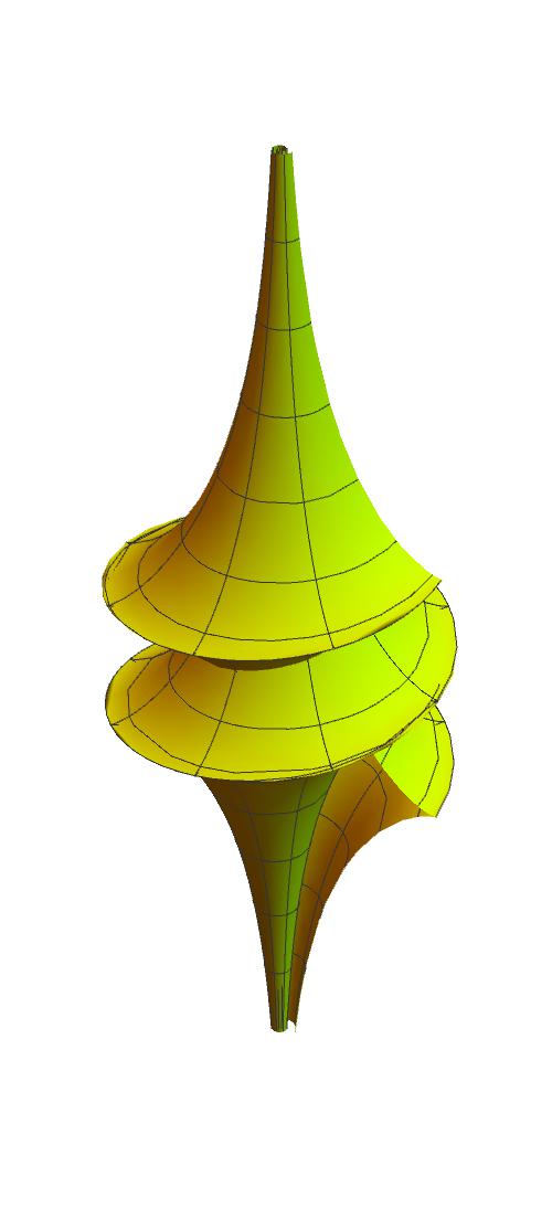
(a)

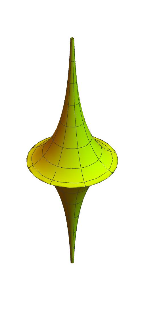
(b)

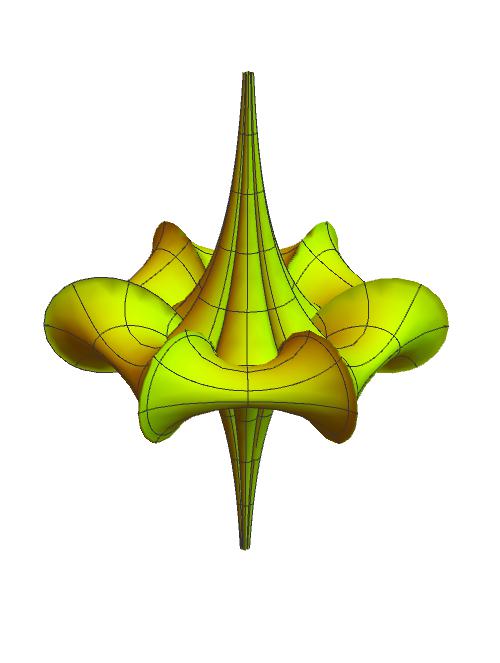
(c)

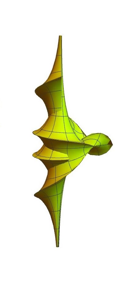
(d)

Figure 1: Pseudo-spherical solitonic surfaces associated to kink and breather solutions. Figure 1a represents the Dini surface, corresponding to a moving kink, while in Figure 1b the famous Beltrami pseudo-sphere is represented. The latter surface is obtained from Dini’s surface by taking the stationary limit of the kink solution. Figures 1c and 1d correspond to the pseudo-spherical surfaces associated to a stationary breather and to a two-kink solution, respectively.

The embedded surfaces in ${\mathbb{R}}^{3}$, as we have just argued and will be explicitly shown in the next section, are independent of the deformation parameter $\tau$, being it re absorbable through a local change of coordinates.

The corresponding soliton solutions, described in section 5, are instead affected by the $\text{T}\bar{\text{T}}$ in a highly non-trivial way. For instance, they generally possess critical values in $\tau$ corresponding to shock-wave phenomena, i.e. branching of the solutions. Examples of shock-wave phenomena and square root-type transitions in the classical energy – similar to the Hagedorn transition at quantum level – will be discussed in sections 5 and 6 for specific solutions of the deformed sine-Gordon model.

3.1 From the deformed to the undeformed model through a local change of coordinates

Thus we have inferred that there must exist a coordinate system $\mathbf{w}=(w^{1}(\mathbf{z}),w^{2}(\mathbf{z}))=\left(w(\mathbf{z}),\bar{w}(\mathbf{z})\right)$ in which the matrices $g_{\mu\nu}^{\text{T}\bar{\text{T}}}$ and $d_{\mu\nu}^{\text{T}\bar{\text{T}}}$ assume the same form as $g_{\mu\nu}^{\textrm{sG}}$ and $d_{\mu\nu}^{\textrm{sG}}$, respectively. In formulae

$$g_{\mu\nu}^{\textrm{sG}}dw^{\mu}dw^{\nu}=g_{\mu\nu}^{\text{T}\bar{\text{T}}}dz^{\mu}dz^{\nu}\;\Longrightarrow\;g_{\mu\nu}^{\textrm{sG}}\frac{dw^{\mu}}{dz^{\rho}}\frac{dw^{\nu}}{dz^{\sigma}}=g_{\rho\sigma}^{\text{T}\bar{\text{T}}}\;,$$ (39)

$$d_{\mu\nu}^{\textrm{sG}}dw^{\mu}dw^{\nu}=d_{\mu\nu}^{\text{T}\bar{\text{T}}}dz^{\mu}dz^{\nu}\;\Longrightarrow\;d_{\mu\nu}^{\textrm{sG}}\frac{dw^{\mu}}{dz^{\rho}}\frac{dw^{\nu}}{dz^{\sigma}}=d_{\rho\sigma}^{\text{T}\bar{\text{T}}}\;.$$ (40)

It is now a matter of simple algebraic manipulations to obtain the following equations for the new coordinates

$$\partial w =\frac{\left(S+1\right)^{2}}{4S\left(1-\tau V\right)}\;,\qquad\bar{\partial}\bar{w}=\frac{\left(S+1\right)^{2}}{4S\left(1-\tau V\right)}\;,$$ (41)

$$\bar{\partial}w =\frac{\tau}{S}\left(\bar{\partial}\phi\right)^{2}\;,\qquad\quad\,\;\;\partial\bar{w}=\frac{\tau}{S}\left(\partial\phi\right)^{2}\;.$$ (42)

Let us now use the latter relations to find the partial derivatives of the field $\phi$ in the coordinates $\mathbf{w}$:

$$\left(\begin{array}[]{c}\partial\phi\\ \bar{\partial}\phi\end{array}\right)=\mathcal{J}\left(\begin{array}[]{c}\partial\phi/\partial w\\ \partial\phi/\partial\bar{w}\end{array}\right)\;,\qquad\mathcal{J}=\left(\begin{array}[]{c c}\partial w&\partial\bar{w}\\ \bar{\partial}w&\bar{\partial}\bar{w}\end{array}\right)\;.$$ (43)

The result is

$$\partial\phi=\frac{1}{1-\tau\left(\mathcal{K}+V\right)}\frac{\partial\phi}{\partial w}\;,\qquad\bar{\partial}\phi=\frac{1}{1-\tau\left(\mathcal{K}+V\right)}\frac{\partial\phi}{\partial\bar{w}}\;,$$ (44)

where we have defined the following function

$$\mathcal{K}=\frac{\partial\phi(\mathbf{w})}{\partial w}\frac{\partial\phi(\mathbf{w})}{\partial\bar{w}}\;.$$ (45)

With the help of (44), we can now find the expression for $S$ in the coordinates $\mathbf{w}$

$$S=\sqrt{1+4\tau\left(1-\tau V\right)\partial\phi\bar{\partial}\phi}=\frac{1+\tau\left(\mathcal{K}-V\right)}{1-\tau\left(\mathcal{K}+V\right)}\;.$$ (46)

We can then write the Jacobian matrix $\mathcal{J}$ and its inverse $\mathcal{J}^{-1}$ in terms of $\mathbf{w}$ as

$$\mathcal{J} = \left(\begin{array}[]{c c}\partial w&\partial\bar{w}\\ \bar{\partial}w&\bar{\partial}\bar{w}\end{array}\right)=\frac{1}{\left(1-\tau V\right)^{2}-\tau^{2}\mathcal{K}^{2}}\left(\begin{array}[]{c c}1-\tau V&\tau\left(\frac{\partial\phi}{\partial w}\right)^{2}\\ \tau\left(\frac{\partial\phi}{\partial\bar{w}}\right)^{2}&1-\tau V\end{array}\right)\;,$$ (51)

$$\mathcal{J}^{-1} = \left(\begin{array}[]{c c}\partial_{w}z&\partial_{w}\bar{z}\\ \partial_{\bar{w}}z&\partial_{\bar{w}}\bar{z}\end{array}\right)=\left(\begin{array}[]{c c}1-\tau V&-\tau\left(\frac{\partial\phi}{\partial w}\right)^{2}\\ -\tau\left(\frac{\partial\phi}{\partial\bar{w}}\right)^{2}&1-\tau V\end{array}\right)\;.$$ (56)

This results allows us to express the partial derivatives of any function $f\left(\mathbf{z}\right)$ as partial derivatives with respect to the new coordinates

$$\left(\begin{array}[]{c}\partial f\\ \bar{\partial}f\end{array}\right)=\mathcal{J}\left(\begin{array}[]{c}\partial f/\partial w\\ \partial f/\partial\bar{w}\end{array}\right)\;,$$ (57)

and we can then apply all the above formulae to the equation (21), obtaining

$$\partial\left(\frac{\bar{\partial}\phi}{S}\right)+\bar{\partial}\left(\frac{\partial\phi}{S}\right) =2\frac{\frac{\partial}{\partial w}\frac{\partial}{\partial\bar{w}}\phi}{\left(1+\tau\left(\mathcal{K}-V\right)\right)^{2}}-2\tau\frac{V^{\prime}}{\left(1-\tau V\right)^{2}-\tau^{2}\mathcal{K}^{2}}\frac{\mathcal{K}}{\left(1+\tau\left(\mathcal{K}-V\right)\right)}\;,$$ (58)

$$\frac{V^{\prime}}{4S}\left(\frac{S+1}{1-\tau V}\right)^{2} =\frac{V^{\prime}}{\left(1-\tau V\right)^{2}-\tau^{2}\mathcal{K}^{2}}\;.$$ (59)

The equality of (58) and (59) yields then

$$\frac{2\frac{\partial}{\partial w}\frac{\partial}{\partial\bar{w}}\phi-V^{\prime}}{\left(1+\tau\left(\mathcal{K}-V\right)\right)^{2}}=0\;.$$ (60)

4 A geometric map for N-boson fields and arbitrary potential

We have seen, in the preceding section, how the $\text{T}\bar{\text{T}}$ deformation of the sine-Gordon model can be interpreted as a field-dependent coordinate transformation. We arrived at this interesting conclusion by exploiting the relation existing amongst ZCR of soliton equations and the classical geometry of surfaces embedded in flat space. Although this connection was pivotal in guiding us to the map (41, 42), from that point on we did not make explicit mention to the form of the potential. In other words, we can consider all formulae from (41) to (60) to be valid for any $2$-dimensional single scalar system.

More generally, the results (51, 60) admit a straightforward generalisation to the case of $N$ bosonic fields $\phi_{i}$, $(i=1,\dots,N)$ interacting with a generic derivative-independent potential $V(\phi_{i})$

$$\mathcal{L}^{(\tau)}_{N}\left(\mathbf{z}\right)=\frac{V}{1-\tau V}+\frac{-1+\sqrt{1+4\bar{\tau}\left(\mathcal{L}^{(0)}_{\text{free}}-\bar{\tau}\mathcal{B}\right)}}{2\bar{\tau}}\;,$$ (61)

$$\quad\mathcal{L}^{(0)}_{\text{free}}=\sum_{i=1}^{N}\partial\phi_{i}\bar{\partial}\phi_{i}\;,\quad\mathcal{B}=|\partial\vec{\phi}\times\bar{\partial}\vec{\phi}|^{2}\;,$$ (62)

with $\bar{\tau}=\tau(1-\tau V)$, arising as a $\text{T}\bar{\text{T}}$-deformation of Conti:2018jho ; Bonelli:2018kik

$$\mathcal{L}^{(0)}_{N}=\sum_{i=1}^{N}\partial\phi_{i}\bar{\partial}\phi_{i}+V(\phi_{i})\;.$$ (63)

The generalization of (51) to the $N$-boson case is

$$\mathcal{J}_{N} = \left(\begin{array}[]{cc}\partial w&\partial\bar{w}\\ \bar{\partial}w&\bar{\partial}\bar{w}\end{array}\right)=\frac{1}{(1-\tau V)^{2}-\tau^{2}\left(\mathcal{K}_{N}\right)^{2}}\left(\begin{array}[]{cc}1-\tau V&\tau\sum_{i=1}^{N}\left(\frac{\partial\phi_{i}}{\partial w}\right)^{2}\\ \tau\sum_{i=1}^{N}\left(\frac{\partial\phi_{i}}{\partial\bar{w}}\right)^{2}&1-\tau V\end{array}\right)\;,$$ (68)

$$\mathcal{J}_{N}^{-1} = \left(\begin{array}[]{cc}\partial_{w}z&\partial_{w}\bar{z}\\ \partial_{\bar{w}}z&\partial_{\bar{w}}\bar{z}\end{array}\right)=\left(\begin{array}[]{cc}1-\tau V&-\tau\sum_{i=1}^{N}\left(\frac{\partial\phi_{i}}{\partial w}\right)^{2}\\ -\tau\sum_{i=1}^{N}\left(\frac{\partial\phi_{i}}{\partial\bar{w}}\right)^{2}&1-\tau V\end{array}\right)\;,$$ (73)

with $\left(\mathcal{K}_{N}\right)^{2}=\sum_{i=1}^{N}\left(\frac{\partial\phi_{i}}{\partial w}\right)^{2}\sum_{i=1}^{N}\left(\frac{\partial\phi_{i}}{\partial\bar{w}}\right)^{2}$. In fact we have verified that the deformed EoMs resulting from (61) are mapped by (68) into the undeformed EoMs associated to $\mathcal{L}^{(0)}_{N}$.
It is instructive to translate (68) in Euclidean coordinates. Considering

$$\left(\frac{\partial}{\partial w}+\frac{\partial}{\partial\bar{w}}\right)(z+\bar{z}) = 2+\tau\left(-\sum_{i=1}^{N}\left(\frac{\partial\phi_{i}}{\partial\bar{w}}\right)^{2}-\sum_{i=1}^{N}\left(\frac{\partial\phi_{i}}{\partial w}\right)^{2}-2V\right)\;,$$

$$\left(\frac{\partial}{\partial w}-\frac{\partial}{\partial\bar{w}}\right)(z-\bar{z}) = 2-\tau\left(\sum_{i=1}^{N}\left(\frac{\partial\phi_{i}}{\partial\bar{w}}\right)^{2}-\sum_{i=1}^{N}\left(\frac{\partial\phi_{i}}{\partial w}\right)^{2}+2V\right)\;,$$

$$\left(\frac{\partial}{\partial w}+\frac{\partial}{\partial\bar{w}}\right)(z-\bar{z}) = \tau\left(\sum_{i=1}^{N}\left(\frac{\partial\phi_{i}}{\partial\bar{w}}\right)^{2}-\sum_{i=1}^{N}\left(\frac{\partial\phi_{i}}{\partial w}\right)^{2}\right)\;,$$

$$\left(\frac{\partial}{\partial w}-\frac{\partial}{\partial\bar{w}}\right)(z+\bar{z}) = -\tau\left(\sum_{i=1}^{N}\left(\frac{\partial\phi_{i}}{\partial\bar{w}}\right)^{2}-\sum_{i=1}^{N}\left(\frac{\partial\phi_{i}}{\partial w}\right)^{2}\right)\;,$$ (74)

and moving to Euclidean coordinates both in the $\mathbf{z}$ and in the $\mathbf{w}$ frames

$$\begin{cases}z=x^{1}+\mathbbm{i}\,x^{2}\\ \bar{z}=x^{1}-\mathbbm{i}\,x^{2}\end{cases}\;,\;\begin{cases}w=y^{1}+\mathbbm{i}\,y^{2}\\ \bar{w}=y^{1}-\mathbbm{i}\,y^{2}\end{cases}\rightarrow\begin{cases}\frac{\partial}{\partial w}+\frac{\partial}{\partial\bar{w}}=\frac{\partial}{\partial y^{1}}\\ \frac{\partial}{\partial w}-\frac{\partial}{\partial\bar{w}}=-\mathbbm{i}\frac{\partial}{\partial y^{2}}\end{cases}$$ (75)

we find

$$\frac{\partial x^{1}}{\partial y^{1}}=1+\tau T^{2}_{\;\;2}(\mathbf{y})\;,\quad\frac{\partial x^{2}}{\partial y^{2}}=1+\tau T^{1}_{\;\;1}(\mathbf{y})\;,\quad\frac{\partial x^{1}}{\partial y^{2}}=\frac{\partial x^{2}}{\partial y^{1}}=-\tau T^{1}_{\;\;2}(\mathbf{y})\;,$$ (76)

where $T^{\mu}_{\;\;\nu}(\mathbf{y})$ is the stress energy tensor of the undeformed theory, $T=T^{(0)}$. Expressions (76) can be more compactly rewritten as

$$\frac{\partial x^{\mu}}{\partial y^{\nu}}=\delta^{\mu}_{\;\;\nu}+\tau\widetilde{T}^{\mu}_{\;\;\nu}(\mathbf{y})\;,\quad\widetilde{T}^{\mu}_{\;\;\nu}(\mathbf{y})=-\epsilon^{\mu}_{\;\;\rho}\epsilon^{\sigma}_{\;\;\nu}T^{\rho}_{\;\;\sigma}(\mathbf{y})\;.$$ (77)

From (77) the inverse Jacobian in Euclidean coordinates reads

$$\mathcal{J}_{N}^{-1}=\left(\begin{array}[]{cc}\frac{\partial x^{1}}{\partial y^{1}}&\frac{\partial x^{2}}{\partial y^{1}}\\ \frac{\partial x^{1}}{\partial y^{2}}&\frac{\partial x^{2}}{\partial y^{2}}\end{array}\right)=\left(\begin{array}[]{cc}1+\tau T^{2}_{\;\;2}&-\tau T^{1}_{\;\;2}\\ -\tau T^{1}_{\;\;2}&1+\tau T^{2}_{\;\;2}\end{array}\right)\;,$$ (78)

and thus the metric, in the set of coordinates $\mathbf{y}$, is

$${\bf g}^{\prime}_{\mu\nu}=\frac{\partial x^{\rho}}{\partial y^{\mu}}\frac{\partial x^{\sigma}}{\partial y^{\nu}}{\bf g}_{\rho\sigma}=\delta_{\mu\nu}-\tau\epsilon_{\mu\rho}\epsilon^{\sigma}_{\;\;\nu}\left(2T+\tau T^{2}\right)^{\rho}_{\;\;\sigma}\;,$$ (79)

where we used the fact that ${\bf g}_{\rho\sigma}=\delta_{\rho\sigma}$. Translating the first expression of (68) in $\mathbf{z}$ coordinates and then moving to Euclidean coordinates, one obtains the inverse relation of (77)

$$\frac{\partial y^{\mu}}{\partial x^{\nu}}=\delta^{\mu}_{\;\;\nu}+\tau\bigl{(}\widetilde{T}^{(\tau)}\bigr{)}^{\mu}_{\;\;\nu}(\mathbf{x})\;,\quad\bigl{(}\widetilde{T}^{(\tau)}\bigr{)}^{\mu}_{\;\;\nu}(\mathbf{x})=-\epsilon^{\mu}_{\;\;\rho}\epsilon^{\sigma}_{\;\;\nu}\bigl{(}T^{(\tau)}\bigr{)}^{\mu}_{\;\;\nu}(\mathbf{x})\;,$$ (80)

where $\bigl{(}T^{(\tau)}\bigr{)}^{\mu}_{\;\;\nu}(\mathbf{x})$ is the stress energy tensor of the deformed theory.
Finally let us conclude this section with a couple of remarks:

• Consider the transformation of the Lagrangian (61) under the on-shell map (68)

  $$\mathcal{L}_{N}^{(\tau)}\left(\mathbf{z}(\mathbf{w})\right)=\frac{\mathcal{L}_{N}^{(0)}(\mathbf{w})+\tau\left(\left(\mathcal{K}_{N}\right)^{2}-V^{2}\right)}{1-2\tau V-\tau^{2}\left(\left(\mathcal{K}_{N}\right)^{2}-V^{2}\right)}\;.$$ (82)

  Using the latter expression together with

  $$\textrm{Det}\left(\mathcal{J}_{N}^{-1}\right)=\textrm{Det}\left(\mathcal{J}_{N}\right)^{-1}=1-2\tau V-\tau^{2}\left(\left(\mathcal{K}_{N}\right)^{2}-V^{2}\right)\;,$$ (83)

  we find that the action transforms as

  $$\mathcal{A}\,[\phi] = \int dz\,d\bar{z}\,\mathcal{L}_{N}^{(\tau)}(\mathbf{z})=\int dw\,d\bar{w}\,\left|\textrm{Det}\left(\mathcal{J}_{N}^{-1}\right)\right|\,\mathcal{L}_{N}^{(\tau)}\left(\mathbf{z}(\mathbf{w})\right)$$ (84)

  $$= \int dw\,d\bar{w}\,\left(\mathcal{L}_{N}^{(0)}(\mathbf{w})+\tau\,\text{T}\bar{\text{T}}^{(0)}(\mathbf{w})\right)\;,$$

  where $\text{T}\bar{\text{T}}^{(0)}(\mathbf{w})=\left(\mathcal{K}_{N}\right)^{2}-V^{2}$. Thus, we conclude that the action is not invariant under the change of variables. This is not totally surprising since the map (68) is on-shell, however it is remarkable that the (bare) perturbing field can be so easily identified once the change of variables is performed. Again, our result matches with Dubovsky:2017cnj , where the $\text{T}\bar{\text{T}}^{(0)}$ term emerges as a JT gravity contribution to the action.

• Notice that the EoMs associated to (61) for a generic potential $V$ are invariant under the transformation

  $$\mathbf{z}\rightarrow\gamma\,\mathbf{z}\;,\quad\tau\rightarrow\gamma\,\tau\;,\quad V\rightarrow V-c\;,$$ (85)

  with $c$ constant and $\gamma=1/(1-\tau c)$, which corresponds to the following change of variables at the level of the solutions

  $$\phi_{i}^{(\tau)}\left(\mathbf{z}\right)\big{|}_{V}=\phi_{i}^{\left(\gamma\,\tau\right)}\left(\gamma\mathbf{z}\right)\big{|}_{V-c}\;,\quad i=1,\dots N\;,$$ (86)

  where the notation $\phi_{i}^{(\tau)}\big{|}_{V}$ means that $\phi_{i}^{(\tau)}$ is solution to the deformed EoMs with potential $V$.

5 $\text{T}\bar{\text{T}}$-deformed soliton solutions in the sine-Gordon model

In this section we show how to compute $\textrm{T}\bar{\textrm{T}}$-deformed solutions of the sG model by explicitly evaluating the change of variables on specific solutions $\phi(\mathbf{w})$ of the undeformed theory. The idea is to solve the following sets of differential equations derived from the inverse Jacobian (51)

$$\begin{cases}\frac{\partial z(\mathbf{w})}{\partial w}=1-\tau V(\phi(\mathbf{w}))\\ \frac{\partial z(\mathbf{w})}{\partial\bar{w}}=-\tau\left(\frac{\partial\phi(\mathbf{w})}{\partial\bar{w}}\right)^{2}\end{cases}\;,\;\begin{cases}\frac{\partial\bar{z}(\mathbf{w})}{\partial w}=-\tau\left(\frac{\partial\phi(\mathbf{w})}{\partial w}\right)^{2}\\ \frac{\partial\bar{z}(\mathbf{w})}{\partial\bar{w}}=1-\tau V(\phi(\mathbf{w}))\end{cases}\;,$$ (87)

for $z(\mathbf{w})$ and $\bar{z}(\mathbf{w})$. Then from the inverse map, i.e. $\mathbf{w}(\mathbf{z})$, we evaluate the expression of the deformed solution as

$$\phi^{(\tau)}(\mathbf{z})=\phi^{(0)}(\mathbf{w}(\mathbf{z}))\;.$$ (88)

In the following we will deal only with some of the simplest solutions of the sG model. In principle our approach applies for all the solutions, although we could not find an explicit result for the integrated map in the cases involving more than two solitons.
For sake of clarity, the computations shown in the following sections will be carried on in light cone coordinates, i.e. $(z,\bar{z})$ and $(w,\bar{w})$, however the plots will be displayed using space and time coordinates $(x,t)=\left(x^{1},x^{2}\right)$.

5.1 The one-kink solution

Let us start with the one-kink solution moving with velocity $v$

$$\phi_{1\text{-kink}}^{(0)}(\mathbf{w})=4\arctan\left(e^{\frac{m}{\beta}\left(aw+\frac{1}{a}\bar{w}\right)}\right)\;,\;a=\sqrt{\frac{1-v}{1+v}}\;.$$ (89)

With the identification $\phi(\mathbf{w})=\phi_{1\text{-kink}}^{(0)}(\mathbf{w})$, equations (87) can be easily integrated yielding

$$z(\mathbf{w}) = w-4\tau\frac{m}{a\,\beta}\tanh{\left[\frac{m}{\beta}\left(aw+\frac{1}{a}\bar{w}\right)\right]}\;,$$

$$\bar{z}(\mathbf{w}) = \bar{w}-4\tau\frac{am}{\beta}\tanh{\left[\frac{m}{\beta}\left(aw+\frac{1}{a}\bar{w}\right)\right]}\;,$$ (90)

where the constants of integration are fixed consistently with the $\tau=0$ case.

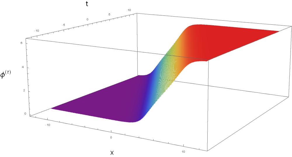
(a)

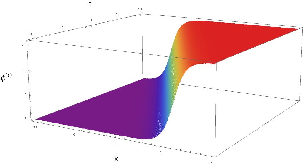
(b)

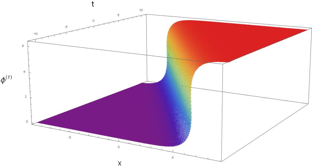
(c)

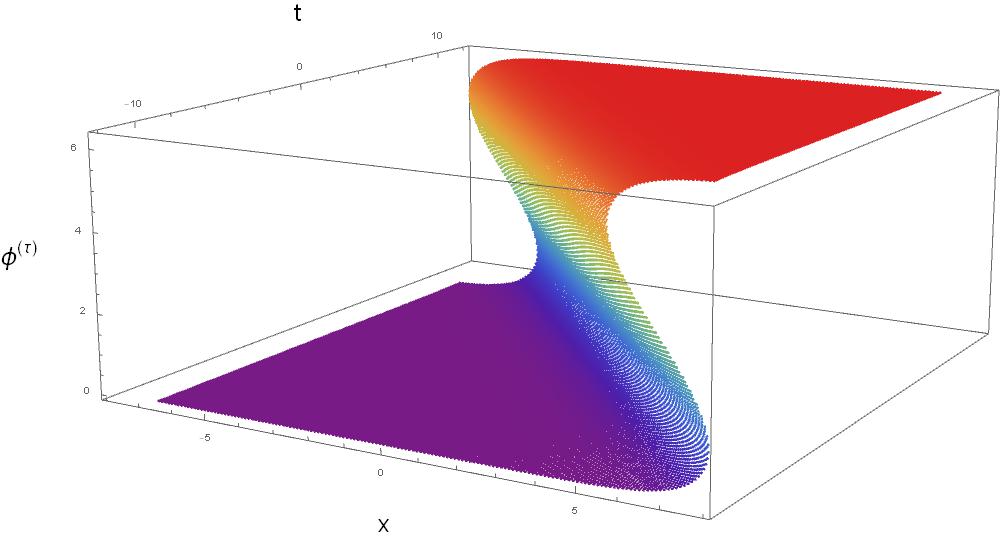
(d)

Figure 2: The $\textsc{T}\bar{\textsc{T}}$-deformed moving one-kink solution $\left(m=\beta=1\,,\,a=2\right)$, for different values of the perturbation parameter $\tau$. Figure 2b represents the undeformed solution. Figure 2a corresponds to $\tau=-1/4$, while Figures 2c and 2d correspond to $\tau=1/8$ and $\tau=1/3$, respectively. Notice that at $\tau=1/8$ a shock-wave singularity occurs.

Notice that from (89) we have

$$\frac{m}{\beta}\left(aw+\frac{1}{a}\bar{w}\right)=\ln{\left(\tan{\left(\frac{\phi_{1\text{-kink}}^{(0)}(\mathbf{w})}{4}\right)}\right)}\;,$$ (91)

and thus expressions (5.1) become

$$z(\mathbf{w})=w+4\tau\frac{m}{a\,\beta}\cos{\left(\frac{\phi_{1\text{-kink}}^{(0)}(\mathbf{w})}{2}\right)}\;,\quad\bar{z}(\mathbf{w})=\bar{w}+4\tau\frac{a\,m}{\beta}\cos{\left(\frac{\phi_{1\text{-kink}}^{(0)}(\mathbf{w})}{2}\right)}\;,$$ (92)

which are easily inverted as

$$w(\mathbf{z}) = z-4\tau\frac{m}{a\,\beta}\cos{\left(\frac{\phi_{1\text{-kink}}^{(0)}\left(\mathbf{w}(\mathbf{z})\right)}{2}\right)}=z-4\tau\frac{m}{a\,\beta}\cos{\left(\frac{\phi_{1\text{-kink}}^{(\tau)}\left(\mathbf{z}\right)}{2}\right)}\;,$$

$$\bar{w}(\mathbf{z}) = \bar{z}-4\tau\frac{am}{\beta}\cos{\left(\frac{\phi_{1\text{-kink}}^{(0)}\left(\mathbf{w}(\mathbf{z})\right)}{2}\right)}=\bar{z}-4\tau\frac{am}{\beta}\cos{\left(\frac{\phi_{1\text{-kink}}^{(\tau)}\left(\mathbf{z}\right)}{2}\right)}\;.$$

Finally, plugging (5.1) into (89) we find

$$\frac{m}{\beta}\left(az+\frac{1}{a}\bar{z}\right)=8\tau\frac{m^{2}}{\beta^{2}}\cos{\left(\frac{\phi_{1\text{-kink}}^{(\tau)}(\mathbf{z})}{2}\right)}+\ln{\left(\tan{\left(\frac{\phi_{1\text{-kink}}^{(\tau)}(\mathbf{z})}{4}\right)}\right)}\;,$$ (94)

which is exactly the deformed one-kink solution found in Conti:2018jho . In Figure 2 the solution is represented for different values of $\tau$. Notice that for negative values of $\tau$ (Figure 2a) the solution stretches w.r.t the undeformed one (Figure 2b), while for positive values of $\tau$ (Figures 2c and 2d) it bends and becomes multi-valued. In particular $\tau=1/8$ (Figure 2c) is the delimiting value corresponding to a shock wave singularity.

5.2 The two-kink solution

Consider now the solution which describes the scattering between two kinks with velocities $v_{1}$ and $v_{2}$

$$\phi_{2\text{-kink}}^{(0)}(\mathbf{w})=4\arctan\left(\frac{a_{1}+a_{2}}{a_{2}-a_{1}}\frac{e^{\frac{m}{\beta}\left(a_{1}w+\frac{1}{a_{1}}\bar{w}+k_{1}\right)}-e^{\frac{m}{\beta}\left(a_{2}w+\frac{1}{a_{2}}\bar{w}+k_{2}\right)}}{1+e^{\frac{m}{\beta}\left(a_{1}w+\frac{1}{a_{1}}\bar{w}+k_{1}\right)}e^{\frac{m}{\beta}\left(a_{2}w+\frac{1}{a_{2}}\bar{w}+k_{2}\right)}}\right)\;,$$ (95)

where again $a_{i}=\sqrt{\frac{1-v_{i}}{1+v_{i}}}\;,\;i=1,2$ , and $k_{i}\;,\;i=1,2$, are constant phases. Compared to the one-kink case, this time the sets of differential equations (87) are more complicated to integrate. It is useful to parametrize the solutions $z(\mathbf{w})$ and $\bar{z}(\mathbf{w})$ of (87) in terms of the combinations

$$u_{i}(\mathbf{w})=\frac{m}{\beta}\left(a_{i}w+\frac{1}{a_{i}}\bar{w}+k_{i}\right)\;,\;i=1,2\;.$$ (96)

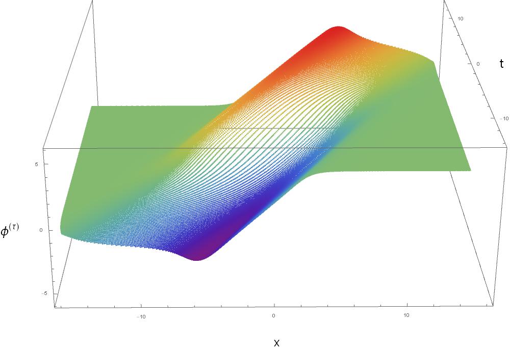
(a)

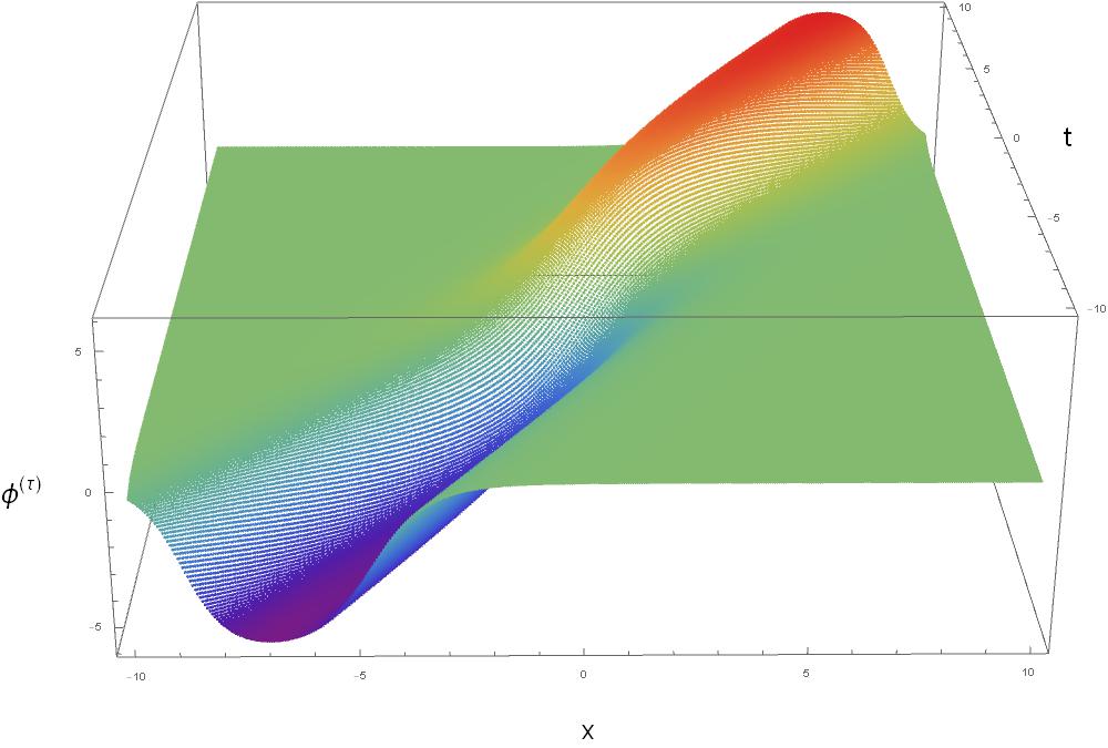
(b)

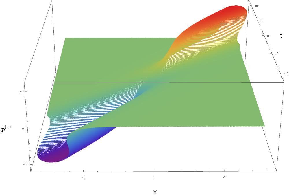
(c)

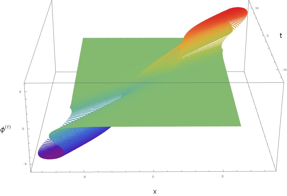
(d)

Figure 3: The $\textsc{T}\bar{\textsc{T}}$-deformed two-kink solution $\left(m=\beta=1\,,\,a_{1}=2\,,\,a_{2}=3\right)$, for different values of the perturbation parameter $\tau$. Figure 3b represents the undeformed solution. Figure 3a corresponds to $\tau=-1/4$, while Figures 3c and 3d correspond to $\tau$, i.e. $\tau=1/10$ and $\tau=1/6$, respectively.

Performing the change of variables $\mathbf{u}=(u_{1}(\mathbf{w}),u_{2}(\mathbf{w}))$

$$\begin{cases}\frac{\partial z}{\partial u_{1}}=\frac{\beta}{m}\frac{a_{1}\left(\frac{\partial z}{\partial w}-a_{2}^{2}\frac{\partial z}{\partial\bar{w}}\right)}{a_{1}^{2}-a_{2}^{2}}\\ \frac{\partial z}{\partial u_{2}}=-\frac{\beta}{m}\frac{a_{2}\left(\frac{\partial z}{\partial w}-a_{1}^{2}\frac{\partial z}{\partial\bar{w}}\right)}{a_{1}^{2}-a_{2}^{2}}\end{cases}\;,\quad\begin{cases}\frac{\partial\bar{z}}{\partial u_{1}}=\frac{\beta}{m}\frac{a_{1}\left(\frac{\partial\bar{z}}{\partial w}-a_{2}^{2}\frac{\partial\bar{z}}{\partial\bar{w}}\right)}{a_{1}^{2}-a_{2}^{2}}\\ \frac{\partial\bar{z}}{\partial u_{2}}=-\frac{\beta}{m}\frac{a_{2}\left(\frac{\partial\bar{z}}{\partial w}-a_{1}^{2}\frac{\partial\bar{z}}{\partial\bar{w}}\right)}{a_{1}^{2}-a_{2}^{2}}\end{cases}\;,$$ (97)

and plugging (87) into (97) with the identification $\phi(\mathbf{w})\equiv\phi_{2\text{-kink}}^{(0)}(\mathbf{w})$, we obtain two sets of differential equations which can be solved for $\mathbf{z}(\mathbf{u})$, giving

$$z(\mathbf{u}) = \frac{\beta}{m}\frac{a_{1}u_{1}-a_{2}u_{2}}{a_{1}^{2}-a_{2}^{2}}-4\tau\frac{m}{\beta}\frac{(a_{1}^{2}-a_{2}^{2})\left(a_{1}\tanh{u_{2}}-a_{2}\tanh{u_{1}}\right)}{a_{1}a_{2}\left(a_{1}^{2}+a_{2}^{2}-2a_{1}a_{2}\left(\operatorname{sech}{u_{1}}\operatorname{sech}{u_{2}}+\tanh{u_{1}}\tanh{u_{2}}\right)\right)}\;,$$

$$\bar{z}(\mathbf{u}) = \frac{\beta}{m}\frac{a_{1}a_{2}\left(a_{1}u_{2}-a_{2}u_{1}\right)}{a_{1}^{2}-a_{2}^{2}}-4\tau\frac{m}{\beta}\frac{(a_{1}^{2}-a_{2}^{2})\left(a_{1}\tanh{u_{1}}-a_{2}\tanh{u_{2}}\right)}{a_{1}^{2}+a_{2}^{2}-2a_{1}a_{2}\left(\operatorname{sech}{u_{1}}\operatorname{sech}{u_{2}}+\tanh{u_{1}}\tanh{u_{2}}\right)}\;.$$

As in the previous section, the constants of integration in (5.2) are fixed by imposing the consistency with the $\tau=0$ case. In order to find the deformed two-kink solution $\phi_{2\text{-kink}}^{(\tau)}\left(\mathbf{z}\right)=\phi_{2\text{-kink}}^{(0)}\left(\mathbf{u}(\mathbf{z})\right)$, we should solve (5.2) for $\mathbf{u}(\mathbf{z})$. Since this is analytically very complicated, we resort to numerical inversion. In Figure 3 the deformed solution $\phi_{2\text{-kink}}^{(\tau)}\left(\mathbf{z}\right)$ is reported for different values of $\tau$. The picture is quite similar to the one-kink case. In fact, for negative values of $\tau$ (Figure 3a) the solution stretches w.r.t. the undeformed one (Figure 3b), while for positive values of $\tau$ (Figures 3c and 3d) it bends and again it becomes multi-valued. Unlike the one-kink case, here it is not possible to find analytically the delimiting value of $\tau$ corresponding to the shock singularity.

5.3 The breather

Another interesting solution is the breather with envelope speed $v=0$

$$\phi_{\text{breather}}^{(0)}(\mathbf{w})=4\arctan\left(\tan{\psi}\,\frac{\sin{\left(-\frac{m}{\beta}(w-\bar{w})\cos{\psi}+\bar{k}\right)}}{\cosh{\left(\frac{m}{\beta}(w+\bar{w})\sin{\psi}+k\right)}}\right)\;,$$ (99)

where $\psi$ is a parameter related to the period $T$ of one full oscillation via $T=\frac{2\pi}{\cos{\psi}}$ and $k,\bar{k}$ are constant phases. In analogy with the two-kink case, it is useful to use the same strategy and parametrize the solutions $\mathbf{z}(\mathbf{w})$ of (87) in terms of

$$u(\mathbf{w})=\frac{m}{\beta}(w+\bar{w})\sin{\psi}+k\;,\quad\bar{u}(\mathbf{w})=-\frac{m}{\beta}(w-\bar{w})\cos{\psi}+\bar{k}\;.$$ (100)

Performing the change of variables $\mathbf{u}(\mathbf{w})=(u(\mathbf{w}),\bar{u}(\mathbf{w}))$, one finds

$$\begin{cases}\frac{\partial z}{\partial u}=\frac{\beta}{m}\frac{1}{2\sin{\psi}}\left(\frac{\partial z}{\partial w}+\frac{\partial z}{\partial\bar{w}}\right)\\ \frac{\partial z}{\partial\bar{u}}=\frac{\beta}{m}\frac{1}{2\cos{\psi}}\left(-\frac{\partial z}{\partial w}+\frac{\partial z}{\partial\bar{w}}\right)\end{cases}\;,\quad\begin{cases}\frac{\partial\bar{z}}{\partial u}=\frac{\beta}{m}\frac{1}{2\sin{\psi}}\left(\frac{\partial\bar{z}}{\partial w}+\frac{\partial\bar{z}}{\partial\bar{w}}\right)\\ \frac{\partial\bar{z}}{\partial\bar{u}}=\frac{\beta}{m}\frac{1}{2\cos{\psi}}\left(-\frac{\partial\bar{z}}{\partial w}+\frac{\partial\bar{z}}{\partial\bar{w}}\right)\end{cases}\;,$$ (101)

and again plugging (87) into (101) with the identification $\phi(\mathbf{w})\equiv\phi_{\text{breather}}^{(0)}(\mathbf{w})$,

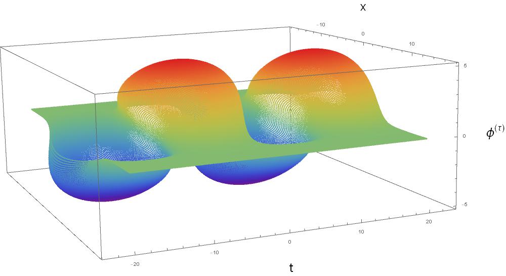
(a)

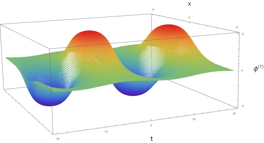
(b)

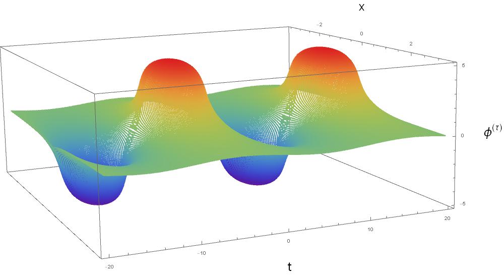
(c)

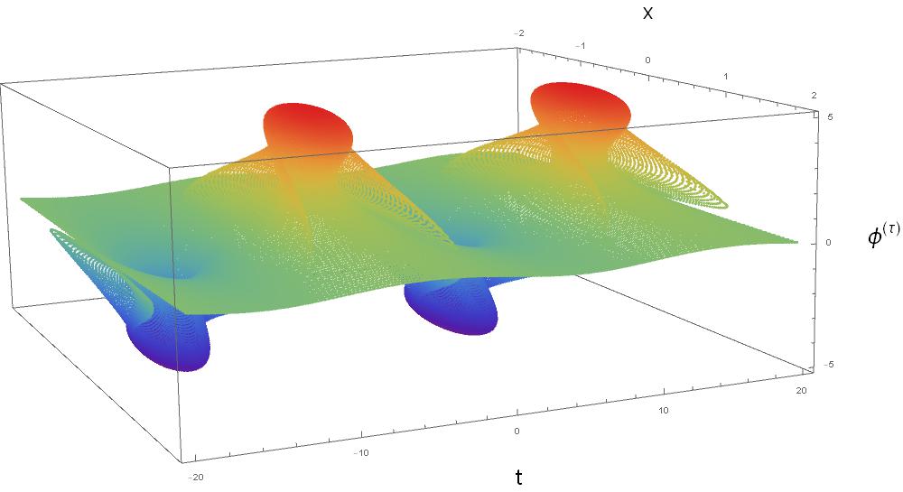
(d)

Figure 4: The $\textsc{T}\bar{\textsc{T}}$-deformed stationary breather solution with envelope speed $v=0$ ($m=\beta=1\,,\,\psi=\frac{2}{5}\pi$), for different values of the perturbation parameter $\tau$. Figure 4b represents the undeformed solution, Figure 4a corresponds to $\tau=-1/2$, while Figures 4c and 4d correspond to $\tau=1/10$ and $\tau=1/5$, respectively.

one gets two sets of differential equations which can be solved for $\mathbf{z}(\mathbf{u})$ giving

$$z(\mathbf{u}) = \frac{\beta}{m}\left(\frac{u}{2\sin{\psi}}-\frac{\bar{u}}{2\cos{\psi}}\right)-8\tau\frac{m}{\beta}\sin{\psi}\frac{\cos{\bar{u}}}{\cosh{u}}\frac{\sec{\bar{u}}\sinh{u}+\operatorname{sech}{u}\sin{\bar{u}}\tan{\psi}}{1+\left(\tan{\psi}\sin{\bar{u}}\operatorname{sech}{u}\right)^{2}}\;,$$

$$\bar{z}(\mathbf{u}) = \frac{\beta}{m}\left(\frac{u}{2\sin{\psi}}+\frac{\bar{u}}{2\cos{\psi}}\right)-8\tau\frac{m}{\beta}\sin{\psi}\frac{\cos{\bar{u}}}{\cosh{u}}\frac{\sec{\bar{u}}\sinh{u}-\operatorname{sech}{u}\sin{\bar{u}}\tan{\psi}}{1+\left(\tan{\psi}\sin{\bar{u}}\operatorname{sech}{u}\right)^{2}}\;.$$

As for the two-kink example, the constants of integration in (5.3) are fixed according to the $\tau=0$ case, and again the solution $\mathbf{u}(\mathbf{z})$ to (5.3) is computed numerically. The deformed solution $\phi_{\text{breather}}^{(\tau)}(\bf z)$ is displayed in Figure 4 for different values of $\tau$. The result is similar to the previous cases: the solution stretches for negative values of $\tau$ (Figure 4a) and it bends for positive values of $\tau$ (Figure 4c and 4d) w.r.t. the undeformed one (Figure 4b). However, notice that in this case the shock phenomenon occurs in both positive and negative directions of $\tau$, and consequently the solution becomes multi-valued (Figures 4a and 4d) for $|\tau|$ sufficiently large.

6 The shock-wave phenomenon and the Hagedorn-type transition

In this section we will discuss the emergence of critical phenomena in the classical solutions, i.e. the shock-wave singularity and the square root-type transition, and comment on the relations among them. We will use as a guide example the stationary $\text{T}\bar{\text{T}}$-deformed elliptic solution of the sG model derived in Conti:2018jho , where we set $\rho=1/\kappa>0$ and $m=\beta=1$,

$$x=\frac{1}{2\sqrt{\rho}}\left[\left(\rho+4\tau\right)\,\mathbf{F}\left(\frac{\phi(x)}{2}\,\vline-\rho\right)-8\tau\,\mathbf{E}\left(\frac{\phi(x)}{2}\,\vline-\rho\right)\right]\;,$$ (103)

defined on a cylinder of radius $R$ fixed. Due to the following properties of the elliptic functions

$$\mathbf{F}(z+n\pi\,|\gamma) = \mathbf{F}(z\,|\gamma)+2n\,\mathbf{K}(\gamma)\;,$$

$$\mathbf{E}(z+n\pi\,|\gamma) = \mathbf{E}(z\,|\gamma)+2n\,\mathbf{E}(\gamma)\;,\quad z,\gamma\in\mathbb{C}\;,\quad n\in\mathbb{Z}\;,$$ (104)

the solution $\phi(x)$ can be interpreted as a stationary 1-kink with twisted boundary conditions

$$\phi(x+R)=\phi(x)+2\pi\;,$$ (105)

where the radius $R$ is

$$R=\frac{1}{\sqrt{\rho}}\,\bigl{(}\left(\rho+4\tau\right)\,\mathbf{K}\left(-\rho\right)-8\tau\,\mathbf{E}\left(-\rho\right)\bigr{)}\;.$$ (106)

We stress that $R$ is kept fixed while $\rho=\rho(\tau,R)$ is considered as a function of $\tau$ and $R$, defined implicitly through (106). Differentiating both sides of (106) w.r.t. $\tau$ and $R$ and solving for $\partial_{\tau}\rho$ and $\partial_{R}\rho$ one finds

$$\partial_{\tau}\rho=-\frac{8\rho\,(1+\rho)\bigl{(}2\mathbf{E}\left(-\rho\right)-\mathbf{K}\left(-\rho\right)\bigr{)}}{(\rho+4\tau)\,\mathbf{E}\left(-\rho\right)}\;,\quad\partial_{R}\rho=\frac{2\rho^{3/2}\,(1+\rho)}{(\rho+4\tau)\,\mathbf{E}\left(-\rho\right)}\;.$$ (107)

We shall now compute the energy on the cylinder. The components of the Hilbert stress-energy tensor $T_{\mu\nu}^{(\tau)}$ are

$$T_{22}^{(\tau)} \equiv \mathcal{H}^{(\tau)}=\frac{V}{1-\tau V}+\frac{1+\tau(1-\tau V)\,\phi_{x}^{2}-S}{2S\,\tau(1-\tau V)}=\frac{2\,(2+\rho V)}{\rho\,(1-2\tau V)-4\tau}\;,$$ (108)

$$T_{12}^{(\tau)} = T_{21}^{(\tau)}\equiv\mathcal{P}^{(\tau)}=-\frac{\phi_{t}\,\phi_{x}}{2S}=0\;,$$ (109)

$$T_{11}^{(\tau)} = -\frac{V}{1-\tau V}-\frac{1-\tau(1-\tau V)\,\phi_{t}^{2}-S}{2S\,\tau(1-\tau V)}=\frac{4}{\rho+4\tau}\;,$$ (110)

where we used the following expressions for $\phi_{t}$ and $\phi_{x}$ derived from (103)

$$\phi_{t}=0\;,\quad\phi_{x}=\frac{2\sqrt{\rho}\,\sqrt{4+\rho V}}{\rho\,(1-2\tau V)-4\tau}\;,$$ (111)

and

$$S=\sqrt{1+\tau(1-\tau V)\left(\phi_{x}^{2}-\phi_{t}^{2}\right)}=\frac{\rho+4\tau}{\rho\,(1-2\tau V)-4\tau}\;.$$ (112)

Notice that the apparent pole singularity at $\tau=1/V$ in $T_{11}^{(\tau)}$ and $T_{22}^{(\tau)}$ disappears once (111) is used in (108) and (110). Finally the energy and momentum at finite volume $R$ are

$$E^{(\tau)} = \int_{x_{0}}^{x_{0}+R}\mathcal{H}^{(\tau)}(x)\,dx=\int_{\phi(x_{0})=0}^{\phi(x_{0}+R)=2\pi}\frac{\mathcal{H}^{(\tau)}(\phi)}{\phi_{x}}\,d\phi=\frac{4}{\sqrt{\rho}}\,\bigl{(}2\,\mathbf{E}(-\rho)-\mathbf{K}(-\rho)\bigr{)}\;,$$ (113)

$$P^{(\tau)} = \int_{x_{0}}^{x_{0}+R}\mathcal{P}^{(\tau)}(x)\,dx=\int_{\phi(x_{0})=0}^{\phi(x_{0}+R)=2\pi}\frac{\mathcal{P}^{(\tau)}(\phi)}{\phi_{x}}\,d\phi=0\;,$$ (114)

$$K^{(\tau)} = \int_{x_{0}}^{x_{0}+R}T_{11}^{(\tau)}(x)\,dx=\int_{\phi(x_{0})=0}^{\phi(x_{0}+R)=2\pi}\frac{T_{11}^{(\tau)}(\phi)}{\phi_{x}}\,d\phi=\frac{4R}{\rho+4\tau}\;,$$ (115)

where $x_{0}=0\,(\text{mod}\,R)$. From (107), (113) and (115) one can prove that the energy fulfils the Burgers equation (1) with $P_{n}=0$

$$\partial_{\tau}E^{(\tau)}=\frac{1}{2}E^{(\tau)}\partial_{R}E^{(\tau)}=-\frac{1}{R}\,\det\left(\int_{x_{0}}^{x_{0}+R}T_{\mu\nu}^{(\tau)}(x)\,dx\right)=-\int_{x_{0}}^{x_{0}+R}\det\left(T_{\mu\nu}^{(\tau)}(x)\right)dx\;,$$ (116)

where the last equality in (116) shows the factorization property of the $\text{T}\bar{\text{T}}$ operator at the classical level. Since the energy $E^{(\tau)}$ fulfils a Burgers equation, it is expected to have a square root-type singularity. The critical radius $R_{c}(\tau)$ corresponds to a value of $R$ such that the first derivative of $E^{(\tau)}(R)$ w.r.t. $R$ diverges. One easily checks that

$$\partial_{R}E^{(\tau)}=-\frac{4}{\rho+4\tau}\;,$$ (118)

thus the first derivative is divergent at the radius $R_{c}(\tau)$ defined through the equation

$$\rho\bigl{(}\tau,R_{c}(\tau)\bigr{)}=-4\tau\;.$$ (119)

According to (106) and (113), the critical radius and the corresponding energy turn out to be

$$R_{c}(\tau)=4\sqrt{-\tau}\,\mathbf{E}\left(4\tau\right)\;,\quad E^{(\tau)}_{c}\equiv E^{(\tau)}(R_{c})=\frac{2}{\sqrt{-\tau}}\,\bigl{(}\mathbf{K}(4\tau)-2\,\mathbf{E}(4\tau)\bigr{)}\;.$$ (120)

To find the behavior of $E^{(\tau)}$ as a function of $R$ close to the branch singularity $R_{c}$, we first expand $R$ and $E^{(\tau)}$ in powers of the small quantity $\varepsilon=\rho+4\tau$

$$R-R_{c} = \frac{R_{c}}{128\tau^{2}\,(1-4\tau)}\,\varepsilon^{2}+\mathcal{O}(\varepsilon^{3})\;,$$

$$E^{(\tau)}-E^{(\tau)}_{c} = \frac{R_{c}}{16\tau^{2}\,(1-4\tau)}\,\varepsilon+\mathcal{O}(\varepsilon^{2})\;,$$ (121)

then, removing $\varepsilon$, one finds

$$E^{(\tau)}-E^{(\tau)}_{c}=\pm\frac{\sqrt{R_{c}}}{\tau\sqrt{2-8\tau}}\,\sqrt{R-R_{c}}+\mathcal{O}\left(R-R_{c}\right)\;,$$ (122)

which gives a square root branch point at $R_{c}$ for the energy.

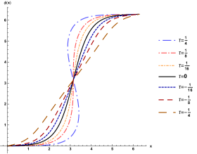
(a)

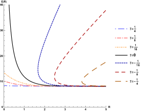
(b)

Figure 5: The kink solution to the $\text{T}\bar{\text{T}}$-deformed sG model on a cylinder of radius $R$ (a) and the corresponding energies as functions of $R$ (b).

Now we would like to briefly discuss the effect of the shock-wave singularities of the deformed solution on the Hamiltonian density. To compute the range of values of $\tau$ where the solution becomes multi-valued, we first identify the zeros of $\text{Det}\left(\mathcal{J}^{-1}\right)$:

$$\text{Det}\left(\mathcal{J}^{-1}\right)=0\quad\Longleftrightarrow\quad x=\frac{\sqrt{\rho}}{2}\,\text{dn}^{-1}\left(\pm\sqrt{\frac{\rho+4\tau}{8\tau}}\;\vline-\rho\right)\;,$$ (123)

where $\text{dn}^{-1}(z\;|\gamma)$ is the inverse of the Jacobi elliptic function $\text{dn}(z\;|\gamma)$. From the reality properties of $\text{dn}^{-1}(z\;|\gamma)$ it follows that $x$ is real for

$$\rho>0\quad\wedge\quad\tau_{1}^{*}=\frac{\rho}{4+8\rho}<\tau<\frac{\rho}{4}=\tau_{2}^{*}\;,$$ (124)

where the critical values $\tau_{1}^{*}$ and $\tau_{2}^{*}$ corresponds to shock-wave singularities of the solution at $\phi=\pi$ and $\phi=0,2\pi$, respectively. The Hamiltonian density (108) is indeed singular when

$$\tau=\frac{\rho}{4+2\rho V}=\frac{\rho}{4+8\rho\,\sin^{2}{(\phi/2)}}\;,$$ (125)

which corresponds to the range of singular values of $\tau$ (124) as $\phi$ interpolates from $0$ to $2\pi$. However, it is important to stress that these branching singularities do not affect the total energy (113), which remains smooth in $\tau$, since the singularities cancel out when dividing by $\phi_{x}$ in (113). In Figure 5 we displayed the behaviour of $\phi(x)$ (Figure 5a) and $E^{(\tau)}(R)$ (Figure 5b) for various values of $\tau$. We see that the shock-wave phenomenon and the square root-type singularity occur at positive and negative values of $\tau$, respectively.

7 Conclusions

Starting from the $\text{T}\bar{\text{T}}$-deformed Lagrangians proposed in Cavaglia:2016oda ; Conti:2018jho ; Bonelli:2018kik , the main result of this article is the direct derivation of the exact one-to-one map between solutions of the unperturbed and deformed equations of motion, which takes the general form (4,5). The result matches the topological gravity predictions of Dubovsky:2017cnj ; Dubovsky:2018bmo but it should be possible to obtain the fundamental equations (4,5,7) also by working within the framework introduced by Cardy in Cardy:2018sdv .

We initially arrived to this conclusion by studying the well known classical relation between sine-Gordon, the associated Lax operators and pseudo-spherical surfaces embedded in ${\mathbb{R}}^{3}$. We think that this alternative and more explicit approach to the problem may provide a complementary point of view compared to Dubovsky:2017cnj ; Dubovsky:2018bmo and open the way to the implementation of further integrable model tools, such as the Inverse Scattering Method and the ODE/IM correspondence within the $\text{T}\bar{\text{T}}$/JT framework.

There are many theoretical aspects that deserve to be further explored. First of all, it would be conceptually very important to study fermionic theories and supersymmetric sigma models. In Bonelli:2018kik , it was argued that for the $\text{T}\bar{\text{T}}$-perturbed Thirring model the Lagrangian truncates at second order in $\tau$, such a truncation is not totally surprising, however the sine-Gordon Lagrangian is instead deformed in an highly non trivial way and it would be nice to identify the mechanism which allows to preserve the quantum equivalence between the two systems. Secondly, it would important to continue the investigation of deformed 2D Yang-Mills Conti:2018jho , along the lines started in the interesting recent work Santilli:2018xux . These studies might also serve as a guide for the inclusion of the $\text{T}\bar{\text{T}}$ inside the Wilson Loop/Scattering Amplitude setup Alday:2009dv ; Alday:2010vh (see also the remarks in the outlook section of Santilli:2018xux ).

Finally, it would also be interesting to study the generalisation of our results to the $\text{J}\bar{\text{T}}$ case described in Bzowski:2018pcy ; Guica:2017lia ; Chakraborty:2018vja ; Apolo:2018qpq ; Aharony:2018ics and to check whether for any of the higher-dimensional models discussed in Cardy:2018sdv ; Bonelli:2018kik ; Taylor:2018xcy ; Conti:2018jho there could exist a map, between deformed and undeformed solutions, similar to equations (4,5).

Note: We have recently been informed that the coordinate map between deformed and undeformed classical Lagrangian systems was also independently introduced by Chih-Kai Chang and studied in an on-going research project involving also Christian Ferko and Savdeep Sethi.

Acknowledgments – We are especially grateful to Sasha Zamolodchikov, Sylvain Lacroix for inspiring discussions and help, and to Sergei Dubovsky for kindly guiding us through the recent literature connecting the $\text{T}\bar{\text{T}}$ perturbation to JT gravity. We also thank Andrea Cavaglià, Riccardo Borsato, Chih-Kai Chang, Yunfeng Jiang, Zohar Komargodski, Marc Magro, Marc Mezei, Leonardo Santilli, Alessandro Sfondrini, István Szécsényi and Miguel Tierz for useful discussions on related topics. This project was partially supported by the INFN project SFT, the EU network GATIS+, NSF Award PHY-1620628, and by the FCT Project PTDC/MAT-PUR/30234/2017 “Irregular connections on algebraic curves and Quantum Field Theory”.

Appendix A Short review on surfaces embedded in $\mathbb{R}^{3}$

The purpose of this appendix is to briefly review the basic concepts related to the classical theory of surfaces embedded in the Euclidean space $\mathbb{R}^{3}$. We will follow the standard constructive approach which can be found, for example, in rogers2002backlund . Let us start by considering a surface $\Sigma$ together with the vector-valued function $\mathbf{r}\left(\mathbf{z}\right)\in\mathbb{R}^{3}$, describing its embedding into $3$-dimensional flat space. It is clear that the two vectors

$$\mathbf{r}_{\mu}=\frac{\partial}{\partial z^{\mu}}\mathbf{r}\;,\quad\mu=1,2\;,$$ (126)

span the tangent plane $T_{P}\Sigma$ to the surface at any non-critical point $P\in\Sigma$. We will disregard the subtleties arising with the presence of critical points and suppose that $\mathbf{r}_{1}\left(\mathbf{z}\right)\neq\mathbf{r}_{2}\left(\mathbf{z}\right)$ for all points $P\in\Sigma$. This basis of $T_{P}\Sigma$ can be improved to a basis $\sigma$ of $\mathbb{R}^{3}$ by adding the unit normal vector $\mathbf{n}$

$$\sigma=\left\{\mathbf{r}_{1},\mathbf{r}_{2},\mathbf{n}\right\}\;,\qquad\mathbf{n}=\frac{\mathbf{r}_{1}\times\mathbf{r}_{2}}{\left|\mathbf{r}_{1}\times\mathbf{r}_{2}\right|}\;.$$ (127)

The surface $\Sigma$ inherits a metric structure from the ambient space $\mathbb{R}^{3}$ and its line element, also known as first fundamental quadratic form, is

$$\textsc{I}\equiv ds^{2}=d\mathbf{r}\cdot d\mathbf{r}=\mathbf{r}_{\mu}\cdot\mathbf{r}_{\nu}dz^{\mu}dz^{\nu}\;.$$ (128)

The tensor

$$g_{\mu\nu}=\mathbf{r}_{\mu}\cdot\mathbf{r}_{\nu}\;,$$ (129)

is called first fundamental tensor or metric tensor of the surface $\Sigma$. According to the classical theorem by Bonnet Bonn_867 any surface embedded in flat $3$-space is uniquely determined, up to isometries, by the first and the second fundamental quadratic form, defined as

$$\textsc{II}=-d\mathbf{r}\cdot d\mathbf{n}=-\mathbf{r}_{\nu}\cdot\left(\frac{\partial}{\partial z^{\mu}}\mathbf{n}\right)\,dz^{\mu}dz^{\nu}=\left(\frac{\partial}{\partial z^{\mu}}\mathbf{r}_{\nu}\right)\cdot\mathbf{n}\,dz^{\mu}dz^{\nu}\;.$$ (130)

The tensor

$$d_{\mu\nu}=\left(\frac{\partial}{\partial z^{\mu}}\mathbf{r}_{\nu}\right)\cdot\mathbf{n}\;,$$ (131)

describes the projection of the vectors $\frac{\partial}{\partial z^{\mu}}\mathbf{r}_{\nu}\left(P\right)$ on the normal direction and tells us how much the surface curves away from the tangent space in an infinitesimal interval around the point $P$. These two tensors can be combined into the object

$$s_{\mu}^{\nu}=d_{\mu\rho}g^{\rho\nu}\;,\qquad g_{\mu\rho}g^{\rho\nu}=\delta_{\mu}^{\nu}\;,$$ (132)

known as shape or Weingarten operator, whose eigenvalues $\kappa_{1},\,\kappa_{2}$ are the principal curvatures of the surface $\Sigma$. The latter quantities are geometric invariants, meaning that they do not change under coordinate transformations. Usually they are combined into the Gauss and mean curvatures

$$K=\kappa_{1}\kappa_{2}=\textrm{Det}\left(s_{\mu}^{\nu}\right)\;,\quad H=\frac{\kappa_{1}+\kappa_{2}}{2}=\frac{1}{2}s_{\mu}^{\mu}\;.$$ (133)

The tensors $g_{\mu\nu}$ and $d_{\mu\nu}$ determine the structural equations for embedded surfaces, comprising the Gauss equations

$$\frac{\partial}{\partial z^{\mu}}\mathbf{r}_{\nu}=\Gamma_{\mu\nu}^{\rho}\mathbf{r}_{\rho}+d_{\mu\nu}\mathbf{n}\;,$$ (134)

and the Weingarten equations

$$\frac{\partial}{\partial z^{\mu}}\mathbf{n}=s_{\mu}^{\nu}\mathbf{r}_{\nu}\;,$$ (135)

where we introduced the Christoffel symbols for the metric

$$\Gamma_{\mu\nu}^{\rho}=\frac{1}{2}g^{\rho\sigma}\left(\frac{\partial}{\partial z^{\nu}}g_{\mu\sigma}+\frac{\partial}{\partial z^{\mu}}g_{\nu\sigma}-\frac{\partial}{\partial z^{\sigma}}g_{\mu\nu}\right)\;.$$ (136)

These equations describe how the frame $\sigma$ moves on the surface and can be collected into the following linear system

$$\frac{\partial}{\partial z^{\mu}}\sigma=U_{\mu}\sigma\;,$$ (137)

with

$$U_{1}=\left(\begin{array}[]{c c c}\Gamma_{11}^{1}&\Gamma_{11}^{2}&d_{11}\\ \Gamma_{12}^{1}&\Gamma_{12}^{2}&d_{12}\\ -s_{1}^{1}&-s_{1}^{2}&0\end{array}\right)\;,\qquad U_{2}=\left(\begin{array}[]{c c c}\Gamma_{12}^{1}&\Gamma_{12}^{2}&d_{12}\\ \Gamma_{22}^{1}&\Gamma_{22}^{2}&d_{22}\\ -s_{2}^{1}&-s_{2}^{2}&0\end{array}\right)\;.$$ (138)

These structural equations are subject to a set of compatibility conditions called Gauss-Mainardi-Codazzi (GMC) system, which takes the form of a zero curvature condition on the matrices $U_{\mu}$

$$\partial_{2}U_{1}-\partial_{1}U_{2}+\left[U_{1},U_{2}\right]=0\;.$$ (139)

Note that the matrices $U_{\mu}$ do not form a Lax pair in the usual sense, since no spectral parameter is present. Moreover, these matrices do not belong to any particular semi-simple Lie algebra. Specialising this general construction to the sine-Gordon case, we will show how to build a proper Lax pair out of the matrices $U_{\mu}$.
As a first example, consider a pseudo-spherical surface. In this case the Gauss curvature is $K=-\mu^{2}<0$, with constant $\mu$, and one can choose as parametric curves the asymptotic lines, for which $d_{11}=d_{22}=0$. Setting $\Delta^{2}=\textrm{Det}\left(g_{\mu\nu}\right)$, we see that

$$K=-\frac{d_{12}^{2}}{\Delta^{2}}\;.$$ (140)

After some manipulations rogers2002backlund , it can be shown that in this case the Mainardi-Codazzi equations imply

$$\Gamma_{12}^{1}=\Gamma_{12}^{2}=0\quad\Longrightarrow\quad\frac{\partial}{\partial z^{2}}\left(g_{11}\right)=\frac{\partial}{\partial z^{1}}\left(g_{22}\right)=0\;.$$ (141)

Defining the angle $\omega$ between the parametric lines as

$$\cos\omega=\frac{g_{12}}{\sqrt{g_{11}g_{22}}}\;,\qquad\sin\omega=\frac{\Delta}{\sqrt{g_{11}g_{22}}}\;,$$ (142)

we have the following expression for the fundamental forms

I $$=g_{11}\left(dz^{1}\right)^{2}+2\sqrt{g_{11}g_{22}}\cos\omega\,dz^{1}dz^{2}+g_{22}\left(dz^{2}\right)^{2}\;,$$ (143)

II $$=2\mu\sqrt{g_{11}g_{22}}\sin\omega\,dz^{1}dz^{2}\;.$$ (144)

Now, given the (anti-)holomorphicity of $g_{11}$ and $g_{22}$ we can rescale the variables $z^{\mu}$ to $z^{\prime\mu}=\sqrt{g_{\mu\mu}}z^{\mu}$ (no summation on repeated indices here) in terms of which one has

I $$=\left(dz^{\prime 1}\right)^{2}-2\cos\omega\,dz^{\prime 1}dz^{\prime 2}+\left(dz^{\prime 2}\right)^{2}\;,$$ (145)

II $$=2\mu\sin\omega\,dz^{\prime 1}dz^{\prime 2}\;.$$ (146)

It is possible to show that the GMC system (139) reduces to the sine-Gordon equation

$$\frac{\partial}{\partial z^{\prime 1}}\frac{\partial}{\partial z^{\prime 2}}\omega=\mu^{2}\sin\omega\;.$$ (147)

Let us now consider the matrices $U_{\mu}$

$$U_{1} = \left(\begin{array}[]{c c c}\omega_{1}\,\cot\omega&-\omega_{1}\,\csc\omega&0\\ 0&0&\mu\sin\omega\\ \mu\cot\omega&-\mu\csc\omega&0\end{array}\right)\;,$$ (151)

$$U_{2} = \left(\begin{array}[]{c c c}0&0&\mu\sin\omega\\ -\omega_{2}\,\csc\omega&\omega_{2}\,\cot\omega&0\\ -\mu\csc\omega&\mu\cot\omega&0\end{array}\right)\;,$$ (155)

where $\omega_{\mu}=\frac{\partial}{\partial z^{\mu}}\omega$. The matrices (151) do not belong to $\mathfrak{su}\left(2\right)$, as we would expect, and contain no trace of the spectral parameter $\lambda$. We can fix these apparent problems by the following considerations. First we notice that the triple $\sigma=\left\{\boldsymbol{r}_{1},\boldsymbol{r}_{2},\boldsymbol{n}\right\}$ is not orthonormal. However, the rotation

$$\sigma\;\longrightarrow\;\tilde{\sigma}=M\sigma\;,\qquad M=\left(\begin{array}[]{c c c}1&0&0\\ -\cot\omega&\csc\omega&0\\ 0&0&1\end{array}\right)\;,$$ (156)

which corresponds to a gauge transformation on the matrices $U_{\mu}$

$$U_{\mu}\;\longrightarrow\;\tilde{U}=\left(\partial_{\mu}M\right)M^{-1}+MU_{\mu}M^{-1}\;,$$ (157)

leaves the compatibility equation – the sine-Gordon equation – invariant and maps (151) into

$$\tilde{U}_{1}=\left(\begin{array}[]{c c c}0&-\omega_{1}&0\\ \omega_{1}&0&\mu\\ 0&-\mu&0\end{array}\right)\;,\qquad\tilde{U}_{2}=\left(\begin{array}[]{c c c}0&0&\mu\sin\omega\\ 0&0&-\mu\cos\omega\\ -\mu\sin\omega&\mu\cos\omega&0\end{array}\right)\;,$$ (158)

which now belong to the $\mathfrak{su}\left(2\right)$ algebra. Finally, the spectral parameter can be recovered by noticing that the sine-Gordon equation is invariant under the following transformation

$$\left(z^{\prime 1},z^{\prime 2},\mu\right)=\left(\alpha\tilde{z}^{1},\beta\tilde{z}^{2},\frac{1}{\sqrt{\alpha\beta}}m\right)\;,$$ (159)

for any constant $\alpha$ and $\beta$. Choosing $\alpha=\sqrt{2}m$ and $\beta=\sqrt{2}\frac{m}{\lambda^{2}}$ and writing $\omega=\beta\phi$, we obtain

I $$=2m^{2}\left(\left(d\tilde{z}^{1}\right)^{2}-\frac{2}{\lambda^{2}}\cos\beta\phi\,d\tilde{z}^{1}d\tilde{z}^{2}+\frac{1}{\lambda^{4}}\left(d\tilde{z}^{2}\right)^{2}\right)\;,$$ (160)

II $$=2\sqrt{2}\frac{m^{2}}{\lambda}\sin\beta\phi\,d\tilde{z}^{1}d\tilde{z}^{2}\;,$$ (161)

which coincides with the quadratic forms (18, 19).
Finally, as another interesting example of integrable model associated to embedded surfaces, let us briefly discuss a constant mean curvature surface, i.e. a surface such that $H=\textrm{const.}$. In this case one can choose conformal coordinates, in which the fundamental forms simplify to

I $$=\frac{2}{H^{2}}e^{\omega}dz^{1}dz^{2}\;,$$ (162)

II $$=\frac{1}{H}\left[A_{1}\left(dz^{1}\right)^{2}+2e^{\omega}dz^{1}dz^{2}+A_{2}\left(dz^{2}\right)^{2}\right]\;.$$ (163)

Some simple computation shows that the GCM equations are equivalent to the system

$$\frac{\partial}{\partial z^{1}}\frac{\partial}{\partial z^{2}}\omega =e^{\omega}-A_{1}A_{2}e^{-\omega}\;,$$ (164)

$$\frac{\partial}{\partial z^{2}}A_{1} =\frac{\partial}{\partial z^{1}}A_{2}=0\;,$$ (165)

which is known as modified sinh-Gordon equation. Its Gauss curvature is

$$K=H^{2}\left(1-A_{1}A_{2}e^{-2\omega}\right)\;.$$ (166)

Rescaling the field as $\omega\rightarrow\omega+2\ln H$, the functions $A_{i}$ as $A_{i}\rightarrow HA_{i}$ and sending $H\rightarrow 0$ yields a minimal surface and reduces the GMC system to Liouville equation

$$\frac{\partial}{\partial z^{1}}\frac{\partial}{\partial z^{2}}\omega=Ke^{\omega}\;,\quad K=-A_{1}A_{2}e^{-2\omega}\;.$$ (167)

Appendix B Computation of the fundamental quadratic forms from sine-Gordon ZCR

While in the preceding appendix we presented the derivation of soliton equations starting from the basic geometric data of some particular surface, here we wish to follow the reverse path and explicitly show how to obtain the forms (18, 19) starting from sine-Gordon ZCR (15, 16). First of all we need to find a basis of $\mathfrak{su}\left(2\right)$ with respect to the Killing form

$$\left(a,b\right)_{K}=\textrm{Tr}\left(\textrm{\bf Ad}(a)\,\textrm{\bf Ad}(b)\right)\;,\quad a,b\in\mathfrak{su}\left(2\right)\;.$$ (168)

In the adjoint representation one has $T^{i}=\textrm{\bf Ad}\left(\mathcal{S}^{i}\right)$, with

$$T^{1}=\left(\begin{array}[]{c c c}0&1&0\\ -1&0&0\\ 0&0&0\end{array}\right)\;,\quad T^{2}=\left(\begin{array}[]{c c c}0&0&-1\\ 0&0&0\\ 1&0&0\end{array}\right)\;,\quad T^{3}=\left(\begin{array}[]{c c c}0&0&0\\ 0&0&1\\ 0&-1&0\end{array}\right)\;,$$ (169)

and

$$\left(T^{i},T^{j}\right)_{K}=-2\delta^{ij}\;.$$ (170)

The orthonormal basis is easily found to be

$$\mathbf{e}^{i}=\frac{\mathbbm{i}}{\sqrt{2}}\mathcal{S}^{i}\;,$$ (171)

and we see that for a pair of matrices $A$ and $B$ belonging to the $2$-dimensional representation of $\mathfrak{su}\left(2\right)$, one has

$$\left(A,B\right)_{K}=4\;\textrm{Tr}\left(AB\right)\;.$$ (172)

Now we need the partial derivatives of $r$ (11)

$$r=\Phi^{-1}\frac{\partial}{\partial\lambda}\Phi\;\Longrightarrow\;\frac{\partial}{\partial z^{\mu}}r=\Phi^{-1}\frac{\partial}{\partial\lambda}\left(L_{\mu}\Phi\right)-\Phi^{-1}L_{\mu}\Phi\Phi^{-1}\frac{\partial}{\partial\lambda}\Phi\;,$$ (173)

where we have used the linear system $\partial_{\mu}\Phi=L_{\mu}\Phi$. We have then

$$\frac{\partial}{\partial z^{\mu}}r=\Phi^{-1}\frac{\partial L_{\mu}}{\partial\lambda}\Phi\;.$$ (174)

We can immediately compute the metric tensor $g_{\mu\nu}$

$$g_{\mu\nu}=\left(\frac{\partial r}{\partial z^{\mu}},\frac{\partial r}{\partial z^{\nu}}\right)_{K}=4\,\textrm{Tr}\left(\frac{\partial r}{\partial z^{\mu}}\frac{\partial r}{\partial z^{\nu}}\right)=4\,\textrm{Tr}\left(\frac{\partial L_{\mu}}{\partial\lambda}\frac{\partial L_{\nu}}{\partial\lambda}\right)\;.$$ (175)

Inserting the expressions (15, 16) we obtain

$$g_{\mu\nu}=2m^{2}\left(\begin{array}[]{c c}1&-\frac{1}{\lambda^{2}}\cos\left(\beta\phi\right)\\ -\frac{1}{\lambda^{2}}\cos\left(\beta\phi\right)&\frac{1}{\lambda^{4}}\end{array}\right)_{\mu\nu}\;.$$ (176)

The second derivatives of $r$ follow from simple computations

$$\frac{\partial}{\partial z^{\mu}}\frac{\partial}{\partial z^{\nu}}r=\Phi^{-1}\left(\frac{\partial}{\partial z^{\nu}}\frac{\partial L_{\mu}}{\partial\lambda}+\left[\frac{\partial L_{\mu}}{\partial\lambda},L_{\nu}\right]\right)\Phi\;.$$ (177)

The matrix version of the unit normal is

$$n=\sum_{i=1}^{3}n_{i}\mathcal{S}^{i}=\frac{1}{2\sqrt{2}}\frac{\left[\frac{\partial r}{\partial z^{1}},\frac{\partial r}{\partial z^{2}}\right]}{\sqrt{\textrm{Det}\left(\left[\frac{\partial r}{\partial z^{1}},\frac{\partial r}{\partial z^{2}}\right]\right)}}\;.$$ (178)

We obtain that

$$\textrm{Det}\left(\left[\frac{\partial r}{\partial z^{1}},\frac{\partial r}{\partial z^{2}}\right]\right)=\left(\frac{m^{2}}{2\lambda^{2}}\sin\left(\beta\phi\right)\right)^{2}\;.$$ (179)

We can finally compute the second fundamental tensor

$$d_{\mu\nu} =\left(\frac{\partial}{\partial z^{\mu}}\frac{\partial}{\partial z^{\nu}}r,n\right)_{K}$$

$$=\frac{1}{\sqrt{2}}\frac{\lambda^{2}}{m^{2}\sin\left(\beta\phi\right)}\textrm{Tr}\left(\left[\frac{\partial L_{1}}{\partial\lambda},\frac{\partial L_{2}}{\partial\lambda}\right]\left(\frac{\partial}{\partial z^{\nu}}\frac{\partial L_{\mu}}{\partial\lambda}+\left[\frac{\partial L_{\mu}}{\partial\lambda},L_{\nu}\right]\right)\right)\;.$$ (180)

The explicit expression is

$$d_{\mu\nu}=\frac{\sqrt{2}m^{2}}{\lambda}\sin\left(\beta\phi\right)\left(\begin{array}[]{c c}0&1\\ 1&0\end{array}\right)\;.$$ (181)

References

• (1) F. A. Smirnov and A. B. Zamolodchikov, On space of integrable quantum field theories, Nucl. Phys. B915 (2017) 363–383 [arXiv:1608.05499].
• (2) A. Cavaglià, S. Negro, I. M. Szécésnyi and R. Tateo, $T\bar{T}$-deformed 2D Quantum Field Theories, JHEP 10 (2016) 112 [arXiv:1608.05534].
• (3) A. B. Zamolodchikov, Expectation value of composite field $T\bar{T}$ in two-dimensional quantum field theory, hep-th/0401146.
• (4) S. Dubovsky, R. Flauger and V. Gorbenko, Solving the Simplest Theory of Quantum Gravity, JHEP 09 (2012) 133 [arXiv:1205.6805].
• (5) S. Dubovsky, R. Flauger and V. Gorbenko, Effective String Theory Revisited, JHEP 09 (2012) 044 [arXiv:1203.1054].
• (6) M. Caselle, D. Fioravanti, F. Gliozzi and R. Tateo, Quantisation of the effective string with TBA, JHEP 07 (2013) 071 [arXiv:1305.1278].
• (7) C. Chen, P. Conkey, S. Dubovsky and G. Hernandez-Chifflet, Undressing Confining Flux Tubes with $T\bar{T}$, arXiv:1808.01339.
• (8) L. McGough, M. Mezei and H. Verlinde, Moving the CFT into the bulk with $T\overline{T}$, JHEP 04 (2018) 010 [arXiv:1611.03470].
• (9) G. Turiaci and H. Verlinde, Towards a 2d QFT Analog of the SYK Model, JHEP 10 (2017) 167 [arXiv:1701.00528].
• (10) A. Giveon, N. Itzhaki and D. Kutasov, $\mathrm{T}\overline{\mathrm{T}}$ and LST, JHEP 07 (2017) 122 [arXiv:1701.05576].
• (11) A. Giveon, N. Itzhaki and D. Kutasov, A solvable irrelevant deformation of AdS3/CFT2, JHEP 12 (2017) 155 [arXiv:1707.05800].
• (12) M. Asrat, A. Giveon, N. Itzhaki and D. Kutasov, Holography Beyond AdS, Nucl. Phys. B932 (2018) 241–253 [arXiv:1711.02690].
• (13) G. Giribet, $T\bar{T}$-deformations, AdS/CFT and correlation functions, JHEP 02 (2018) 114 [arXiv:1711.02716].
• (14) P. Kraus, J. Liu and D. Marolf, Cutoff AdS3 versus the $T\overline{T}$ deformation, JHEP 07 (2018) 027 [arXiv:1801.02714].
• (15) W. Cottrell and A. Hashimoto, Comments on $T\bar{T}$ double trace deformations and boundary conditions, arXiv:1801.09708.
• (16) M. Baggio and A. Sfondrini, Strings on NS-NS Backgrounds as Integrable Deformations, Phys. Rev. D98 (2018), no. 2 021902 [arXiv:1804.01998].
• (17) J. P. Babaro, V. F. Foit, G. Giribet and M. Leoni, $T\overline{T}$ type deformation in the presence of a boundary, JHEP 08 (2018) 096 [arXiv:1806.10713].
• (18) S. Dubovsky, V. Gorbenko and M. Mirbabayi, Asymptotic fragility, near AdS2 holography and $T\overline{T}$, JHEP 09 (2017) 136 [arXiv:1706.06604].
• (19) G. Mussardo and P. Simon, Bosonic type S matrix, vacuum instability and CDD ambiguities, Nucl. Phys. B578 (2000) 527–551 [hep-th/9903072].
• (20) Al. B. Zamolodchikov, From tricritical Ising to critical Ising by thermodynamic Bethe ansatz, Nucl. Phys. B358 (1991) 524–546.
• (21) S. Dubovsky, V. Gorbenko and M. Mirbabayi, Natural Tuning: Towards A Proof of Concept, JHEP 09 (2013) 045 [arXiv:1305.6939].
• (22) J. Cardy, The $T\overline{T}$ deformation of quantum field theory as a stochastic process, arXiv:1801.06895.
• (23) S. Dubovsky, V. Gorbenko and G. Hernandez-Chifflet, $T\overline{T}$ partition function from topological gravity, JHEP 09 (2018) 158 [arXiv:1805.07386].
• (24) S. Datta and Y. Jiang, $T\bar{T}$ deformed partition functions, JHEP 08 (2018) 106 [arXiv:1806.07426].
• (25) O. Aharony, S. Datta, A. Giveon, Y. Jiang and D. Kutasov, Modular invariance and uniqueness of $T\bar{T}$ deformed CFT, arXiv:1808.02492.
• (26) G. Bonelli, N. Doroud and M. Zhu, $T\bar{T}$-deformations in closed form, JHEP 06 (2018) 149 [arXiv:1804.10967].
• (27) R. Conti, L. Iannella, S. Negro and R. Tateo, Generalised Born-Infeld models, Lax operators and the $\mathrm{T}\overline{\mathrm{T}}$ perturbation, JHEP 11 (2018) 007 [arXiv:1806.11515].
• (28) A. Dei and A. Sfondrini, Integrable spin chain for stringy Wess-Zumino-Witten models, JHEP 07 (2018) 109 [arXiv:1806.00422].
• (29) P. Dorey and R. Tateo, Anharmonic oscillators, the thermodynamic Bethe ansatz, and nonlinear integral equations, J. Phys. A32 (1999) L419–L425 [hep-th/9812211].
• (30) V. V. Bazhanov, S. L. Lukyanov and A. B. Zamolodchikov, Spectral determinants for Schrodinger equation and Q operators of conformal field theory, J. Statist. Phys. 102 (2001) 567–576 [hep-th/9812247].
• (31) P. Dorey, C. Dunning and R. Tateo, The ODE/IM Correspondence, J. Phys. A40 (2007) R205 [hep-th/0703066].
• (32) S. L. Lukyanov and A. B. Zamolodchikov, Quantum Sine(h)-Gordon Model and Classical Integrable Equations, JHEP 07 (2010) 008 [arXiv:1003.5333].
• (33) P. Dorey, S. Faldella, S. Negro and R. Tateo, The Bethe Ansatz and the Tzitzeica-Bullough-Dodd equation, Phil. Trans. Roy. Soc. Lond. A371 (2013) 20120052 [arXiv:1209.5517].
• (34) L. F. Alday, D. Gaiotto and J. Maldacena, Thermodynamic Bubble Ansatz, JHEP 09 (2011) 032 [arXiv:0911.4708].
• (35) L. F. Alday, J. Maldacena, A. Sever and P. Vieira, Y-system for Scattering Amplitudes, J. Phys. A43 (2010) 485401 [arXiv:1002.2459].
• (36) D. Gaiotto, Opers and TBA, arXiv:1403.6137.
• (37) K. Ito and H. Shu, ODE/IM correspondence and the Argyres-Douglas theory, JHEP 08 (2017) 071 [arXiv:1707.03596].
• (38) A. Grassi and M. Mariño, A Solvable Deformation Of Quantum Mechanics, arXiv:1806.01407.
• (39) P. Goddard, J. Goldstone, C. Rebbi and C. B. Thorn, Quantum dynamics of a massless relativistic string, Nucl. Phys. B56 (1973) 109–135.
• (40) E. Bour, Théorie de la déformation des surfaces, J. de l’Ècole Imperiale Polytech. 19 (1862) 1–48.
• (41) J. Liouville, Sur l’équation aux différences partielles $\frac{d^{2}\ln\lambda}{dudv}\pm\frac{\lambda}{2a^{2}}=0$, J. de mathèmatiques pures et appliquèes 18 (1853) 71–72.
• (42) P. O. Bonnet, Mémoire sur la théorie des surfaces applicables sur une surface donnée, J. de l’Ècole Polytech. 42 (1867) 1–151.
• (43) K. Pohlmeyer, Integrable Hamiltonian Systems and Interactions through Quadratic Constraints, Commun. math. Phys. 46 (1976) 207–221.
• (44) F. Lund and T. Regge, Unified approach to strings and vortices with soliton solutions, Phys. Rev. D 14 (1976) 1524–1535.
• (45) B. S. Getmanov, New Lorentz-invariant system with exact multisoliton solutions, JETP Lett. 25 (1977) 119–122.
• (46) A. Sym, Soliton Surfaces, Lett. al Nuovo Cimento 33 (1982) 394–400.
• (47) A. Sym, Soliton Surfaces. II. Geometric Unification of Solvable Nonlinearities, Lett. al Nuovo Cimento 36 (1983) 307–312.
• (48) A. Sym, Soliton Surfaces. III. Solvable nonlinearities with trivial geometry., Lett. al Nuovo Cimento 39 (1984) 193–196.
• (49) A. Sym, Soliton Surfaces. VI. Gauge Invarianee and Final Formulation of the Approach., Lett. al Nuovo Cimento 41 (1984) 353–360.
• (50) A. Sym, Soliton Surfaces. V. Geometric Theory of Loop Solitons., Lett. al Nuovo Cimento 41 (1984) 33–40.
• (51) C. Rogers and W. Schief, Bäcklund and Darboux transformations: geometry and modern applications in soliton theory, vol. 30. Cambridge University Press, 2002.
• (52) L. Santilli and M. Tierz, Large $N$ phase transition in $T\overline{T}$-deformed $2d$ Yang-Mills theory on the sphere, arXiv:1810.05404.
• (53) A. Bzowski and M. Guica, The holographic interpretation of $J\bar{T}$-deformed CFTs, arXiv:1803.09753.
• (54) M. Guica, An integrable Lorentz-breaking deformation of two-dimensional CFTs, arXiv:1710.08415.
• (55) S. Chakraborty, A. Giveon and D. Kutasov, $J\overline{T}$ deformed CFT2 and string theory, JHEP 10 (2018) 057 [arXiv:1806.09667].
• (56) L. Apolo and W. Song, Strings on warped AdS3 via $T\bar{J}$ deformations, arXiv:1806.10127.
• (57) O. Aharony, S. Datta, A. Giveon, Y. Jiang and D. Kutasov, Modular covariance and uniqueness of $J\bar{T}$ deformed CFTs, arXiv:1808.08978.
• (58) M. Taylor, TT deformations in general dimensions, arXiv:1805.10287.