Evaluating Federal Policies Using Bayesian Time Series Models: Estimating the Causal Impact of the Hospital Readmissions Reduction Program

Abstract

Researchers are often faced with evaluating the effect of a policy or program that was simultaneously initiated across an entire population of units at a single point in time, and its effects over the targeted population can manifest at any time period afterwards. In the presence of data measured over time, Bayesian time series models have been used to impute what would have happened after the policy was initiated, had the policy not taken place, in order to estimate causal effects. However, the considerations regarding the definition of the target estimands, the underlying assumptions, the plausibility of such assumptions, and the choice of an appropriate model have not been thoroughly investigated. In this paper, we establish useful estimands for the evaluation of large-scale policies. We discuss that imputation of missing potential outcomes relies on an assumption which, even though untestable, can be partially evaluated using observed data. We illustrate an approach to evaluate this key causal assumption and facilitate model elicitation based on data from the time interval before policy initiation and using classic statistical techniques. As an illustration, we study the Hospital Readmissions Reduction Program (HRRP), a US federal intervention aiming to improve health outcomes for patients with pneumonia, acute myocardial infraction, or congestive failure admitted to a hospital. We evaluate the effect of the HRRP on population mortality among the elderly across the US and in four geographic subregions, and at different time windows. We find that the HRRP increased mortality from pneumonia and acute myocardial infraction across at least one geographical region and time horizon, and is likely to have had a detrimental effect on public health.

keywords: Bayesian methods, causal inference, hospital readmissions reduction program, mortality, policy evaluation, time-series

1 Introduction

Researchers and policy makers are often interested in understanding the effect of new policies or programs. The target policy is often rolled out at once over the whole region of interest, it alters the operation of a group of organizations, which might affect the region’s population in a number of ways. To evaluate the policy, available data include a time period before policy rollout (the “pre-intervention” period), and a time period after policy initiation (the “post-intervention” period). Considering that the policy rollout is experienced by everyone in the region, policy evaluation should also target the policy’s impact on the whole population. Therefore, we are faced with estimating the causal effect of a policy over a single unit measured over time, including a pre- and a post-intervention time period.

In the presence of pre- and post-intervention data, popular methods include the difference-in-difference (Athey and Imbens, 2006) and synthetic control (Doudchenko and Imbens, 2017) approaches. However, these approaches require the presence of control units during both time periods, whereas in our case, everyone is exposed to the policy once it is initiated. Other measured time series for the same population have been previously used as assumed control units in synthetic control methodology (Gaughan et al., 2019). Interrupted (or quasi-experimental) time-series analysis has been alternatively used for estimating causal effects from a single time series (McDowall et al., 2019), but it requires that we correctly specify the outcome model in both the pre- and in the post-intervention time period, an assumption that is rather restrictive. Bojinov and Shephard (2019) introduced causal estimands and estimation based on a single time series, but their methodology requires that the treatment can be applied and taken away at any time point, which is not true for policy settings where once the policy is initiated it remains active throughout.

In this manuscript, we suggest using the whole region where the intervention took place as a single system (unit) for policy evaluation. Under the potential outcome framework for causal inference, we define causal estimands that describe the effect of the policy on the whole system, and introduce the crucial causal assumptions for estimating these quantities using observed data. For estimation, we employ Bayesian time series modeling to impute what would have happened in the post-intervention time period, had the intervention not taken place, and we combine these imputations with observed outcomes to unbiasedly estimate causal effects, similarly to other approaches in the literature (Brodersen et al., 2015; Miratrix et al., 2019; Antonelli and Beck, 2020). We illustrate how model choice and the plausibility of the causal assumptions can be partially evaluated using data from the pre-intervention time period and classic statistical techniques, and using time series data that are expected to be unaffected by the intervention. The framework presented here provides guidance for the evaluation of programs and policies of various sorts, such as educational policies, social programs, or environmental policies that are adopted by schools, neighborhoods, and polluting sources, respectively, and affect the outcomes of the region’s population (Zigler and Papadogeorgou, 2021).

This work is motivated by the evaluation of the Hospital Readmissions Reduction Program (HRRP), part of the Affordable Care Act which passed in 2010. The HRRP created the prospect of financial penalties that would start being applied in 2012 based on risk-standardized readmission rates for Medicare fee-for-service patients within 30 days of discharge after index hospitalization for acute myocardial infarction (AMI), congestive heart failure (CHF), or pneumonia. The HRRP reflected intent to incentivize providers and hospitals to improve the coordination and quality of care for patients. Even though the law was associated with substantial declines in risk-standardized readmissions (Zuckerman et al., 2016; Desai et al., 2016; Wasfy et al., 2017; MedPAC, 2018), whether the law was associated with increased mortality is very controversial (Joynt et al., 2011; Joynt and Jha, 2012; Fonarow et al., 2017) with studies returning drastically different results (Gupta et al., 2017; Dharmarajan et al., 2017; Wadhera et al., 2018; Khera et al., 2018; Huckfeldt et al., 2019; Sandhu and Heidenreich, 2019). Improving our understanding of the causal effects of the HRRP is critical, because this type of information will inform whether similar policies should be implemented or not in the future. Although most of the aforementioned papers adopt methodologies that are often employed in the causal inference literature (e.g., interrupted time series), the underlying assumptions are not explicit and the estimands are not clearly defined. This is necessary to give a reader an understanding of the effect one is aiming to estimate and under which assumptions it can be interpreted as “causal.” Within our framework, we define and estimate the causal effect of the HRRP on mortality from AMI, CHF or pneumonia among individuals that were 65 years old or older across the United States and in four subregions, and at three time windows after the passage of the law. We find that the HRRP caused an increase in mortality from AMI across the US and from pneumonia in some geographical subregions.

2 Methods

2.1 Evaluating a policy at the same level of its scope

For ease of illustration, we focus on the HRRP throughout as a policy which affects hospital operations in an effort to improve public health. To evaluate such a policy, the prevailing analysis approach compares the outcomes of hospitals that were affected by the policy at varying degrees. However, such an analysis is faced with many challenges. Firstly, hospitals that adopt the policy at different degrees can have systematic differences due to both measured and unmeasured factors which might confound the estimation of causal effects on hospital-level outcomes. Second, the extent to which a hospital adopts the policy might affect the outcome of other hospitals, giving rise to interference, which complicates how causal effects are both defined and estimated. That can happen if, for example, hospitals with high financial penalties under the HRRP avoid admitting high-risk patients, who are afterwards admitted at a different hospital (Casalino et al., 2007). Lastly, even if effects of the intervention on hospital-level outcomes were properly defined and estimated, they would represent the effects of policy adoption of different degrees rather than the total effect of the policy, and conclusions on population-level effects based on the analysis of hospital-level outcomes might suffer from ecological bias.

Understanding the effects of policy adoption at different degrees can be essential for uncovering key features of the policy, but the challenges in the analysis of hospital-level data presented above have not been definitively resolved and interpretation of estimated quantities remains complicated. Here, we advocate a complementary approach that bypasses those specific issues in focusing on different, but related, causal estimands. We suggest that evaluation of large-scale policies is performed at the level of the whole population, by viewing the whole region as one system measured over time, and considering causal estimands that describe the change in the outcome over the whole population in the presence and in the absence of the intervention. As we discuss below, this entails notions of confounding that do not necessarily require adjustment for measured differences. It also bypasses the issue of interference, since the whole population composes a single unit that is treated by the policy, and we observe the outcome at an aggregate level irrespective of which hospital provided care to whom. Finally, and importantly for policy evaluation, the framework below allows us to quantify the effect of the policy directly on the population under study, and therefore does not suffer from ecological biases. We find that providing a complimentary way to evaluate large-scale policies by shifting the goalpost from hospital-level analyses to focusing on estimands over the whole population is a key contribution of our work.

2.2 Causal estimands in single time series with one interventional time point

Since the policy could have been passed or not, we formulate our causal estimands using two potential time series: one representing the outcome had the policy taken place, which is observed, and one representing the outcome had the policy not taken place, which is not observed and has to be estimated.

Let $t\in\mathcal{T}=\{1,2,\dots,T\}$ represent $T$ time periods of observed data, and $t^{*}\in\mathcal{T}$ denote the time period during which the policy was actually initiated. Let $w_{t}=1$ denote that the policy is active at time period $t$, and $w_{t}=0$ that it is not. Then,

$$\overline{w}_{1T}=(w_{1}=0,w_{2}=0,\dots,w_{t^{*}-1}=0,w_{t^{*}}=1,w_{t^{*}+1}=1,\dots,w_{T}=1)$$ (1)

represents the observed scenario where the policy is initiated at time $t^{*}$ and remains active thereafter, and

$$\overline{w}_{0T}=(w_{1}=0,w_{2}=0,\dots,w_{t^{*}-1}=0,w_{t^{*}}=0,w_{t^{*}+1}=0,\dots,w_{T}=0)$$ (2)

represents the counterfactual scenario where the policy is never initiated. We postulate the existence of potential outcomes $Y^{jt}=Y^{t}\big{(}\overline{w}_{jT}\big{)}$ for $j\in\{0,1\}$, which represent the population outcome that would have been observed at time period $t$ had the policy never been initiated, or had it been initiated at $t^{*}$, respectively. Then, $Y^{1t}-Y^{0t}$ represents the effect of initiating the policy at time $t^{*}$ against not initiating it at all on the outcome at time period $t$, similarly to the causal estimands in the synthetic control literature (e.g., Doudchenko and Imbens, 2017). We focus at time periods after policy initiation, $t\geq t^{*}$. Then, the causal effect of the policy $k$ time periods after initiation is defined as

$$\Delta_{k}=Y^{1(t^{*}+k)}-Y^{0(t^{*}+k)},\ k\geq 0,$$ (3)

and the cumulative effect during the first $K$ time periods is defined as

$$C\Delta_{K}=\sum_{k=0}^{K-1}\Delta_{k}=\sum_{k=0}^{K-1}\Big{[}Y^{1(t^{*}+k)}-Y^{0(t^{*}+k)}\Big{]}.$$ (4)

In our study, the potential outcomes $Y^{jt}$ represent the total number of deaths across the US had the HRRP passed or not, and the cumulative effect in Equation 4 represents the number of deaths caused or prevented by the policy within $K$ time periods from its initiation.

Defining potential outcomes at the level of the whole region obviates the need to consider interference explicitly. In contrast, hospital-level potential outcomes should be indexed by the treatments of all hospitals which interfere with it, which would complicate the definition of subsequent hospital-level estimands. As also highlighted in Imbens and Rubin (2015), a common strategy to deal with interference between statistical units is changing the level of analysis. Therefore, considering the whole region under study as one unit for which the policy would either take place or not allows us to bypass this issue.

2.3 The causal assumptions

Since the policy was indeed initiated at time period $t^{*}$, the observed treatment is equal to the treatment path $\overline{w}_{1T}$, and the observed outcome $Y_{t}$ is equal to the corresponding potential outcome, $Y_{t}=Y^{1t}$. This implies that all potential outcomes corresponding to the treatment path $\overline{w}_{1T}$ are observed, as illustrated in the top row of Table 1. Therefore, all potential outcomes $Y^{1t}$ in the estimands (3), (4) are observed, and we are faced with estimating the potential outcomes $Y^{0t}$ in the post-intervention period, $t\geq t^{*}$. To do so, we make the following assumptions. The interpretation of these assumptions as well as how we can assess their plausibility is discussed in more detail in Sections 2.4 and 2.5, and within the context of our study in Section 3.2.

Assumption 1.

The policy does not alter potential outcomes before its initiation, $Y^{0t}=Y^{1t}$ for $t<t^{*}$.

1 states that the intervention could not have affected the outcome before it was actually initiated. Therefore, potential outcomes in the pre-intervention time period are the same, irrespective of whether the policy is initiated or not in the future. This assumption establishes that the observed outcomes in the pre-intervention period are equal to the potential outcomes in the absence of the intervention, $Y^{0t}=Y_{t}$ for $t<t^{*}$. The next assumption allows us to use the pre-intervention outcomes to learn the outcome process in the absence of the treatment, potentially conditional on covariates, and is discussed in more detail in Section 2.4.

Table 1: Potential outcomes in the pre- and post-intervention time period, and the causal assumptions.

	pre-intervention period $t<t^{*}$	post-intervention period $t\geq t^{*}$
$Y^{1t}$	observed	observed
$Y^{0t}$	$=$ observed (1)	imputed based on 2

Assumption 2.

There exist measured covariates $X_{t}$ which are unaltered by the intervention, and conditional on which the outcome process is stationary with some lag $M\geq 0$, i.e. if $X^{jt}=X^{t}(\overline{w}_{jT})$ are the potential covariate values under treatment path $\overline{w}_{jT}$ for $j=0,1$, we have that $X^{0t}=X^{1t}$, and there exists $M\geq 0$ such that, for all $t\in\mathcal{T}$,

$$P(Y^{0t}|Y^{0(t-1)},\dots,Y^{0(t-M)},X^{0t},\dots,X^{0(t-M+1)})$$

$$\hskip 20.0pt=P(Y^{0(t+1)}|Y^{0t},\dots,Y^{0(t-M+1)},X^{0(t+1)},\dots,X^{0(t-M+2)}).$$

2 is the basis for imputing the missing potential outcomes in the absence of the policy. For illustration, assume that it holds for $M=1$ and in the absence of covariates. Then, the conditional outcome distribution is the same for all time points in the pre-intervention period, i.e. for $t_{1},t_{2}<t^{*}$ it holds that $P(Y^{0t_{1}}|Y^{0(t_{1}-1)})=P(Y^{0t_{2}}|Y^{0(t_{2}-1)})$. Since the potential outcomes $Y^{0t}$ in the pre-intervention period are observed from 1, this conditional distribution can be estimated from the data. Then, setting $t=t^{*}$ in 2, we have $P(Y^{0t^{*}}|Y^{0(t^{*}-1)})=P(Y^{0(t^{*}-1)}|Y^{0(t^{*}-2)})$ which allows us to impute $Y^{0t^{*}}$. Once $Y^{0t^{*}}$ is imputed based on this distribution, the same statement for $t=t^{*}+1$ will be used to impute $Y^{0(t^{*}+1)}$ and so forth. Therefore, 2 enables us to learn the potential outcome process using the observed outcomes in the pre-intervention period, and use it to predict the missing potential outcomes in the post-intervention period had the policy not taken place.

2.4 Confounding with a single unit measured over time

Here, we start by discussing the notion of confounding in the setting of a single unit followed over time, and then we relate it to our 2. An analogous discussion in the context of multiple units measured over time is given in Antonelli and Beck (2020).

In most settings in causal inference, measured covariates are assumed to satisfy a no-unmeasured confounding assumption in that they represent all the ways in which treated and control units differ, and that, within cells defined by these covariates, treatment assignment is independent of any potential outcome. In our setting, the whole system is viewed as a single unit subject to the intervention for which we have access to a time period before the intervention when the unit is untreated, and a time period after the intervention when the unit is treated. Construing the different time periods as the most primitive observational units, confounding would represent systematic differences in the pre- and post-intervention time periods. Then, the primary threat to validity with estimating the missing potential outcome $Y^{0t}$ in the post-intervention time period is parsing changes due to the policy from other temporal changes that would have occurred regardless. In the HRRP, this could correspond to secular trends in population lifestyle factors or improvements in medical care technology that are not related to the policy, but may have changed mortality outcomes over time. To estimate the causal effect by comparing the outcomes in the pre- and post-intervention time period, we would have to account for all such variables through matching, sub-classification, regression, or other methods.

Rather than finding pre- and post intervention time points with similar values of covariates (which would not generally be available) to account for factors that vary coincidentally with the policy and outcomes, 2 focuses on the potential outcomes in the absence of the intervention and states that secular and periodic trends in the pre-intervention outcome time-series would have persisted in the post-intervention period, had the intervention not taken place. Therefore, this assumption could be satisfied if temporal trends in the pre-intervention time period are properly accommodated using flexible functions of time or covariates. Flexible functions of time can be used to account for the overall decreasing trends in mortality during the pre-intervention period reported in Figure S.2, without requiring to have access to all variables that might drive these trends. In fact, flexible temporal trends can adequately capture covariate time series that predict the outcome and have long term temporal trends, such as population comorbidities which have overall persistent trends during our study period. Therefore, the assumption might hold without any covariates, in which case covariates are not needed for unbiased estimation of causal effects. However, researchers have to be mindful to include covariates that predict the outcome time series and have a temporal pattern that changes post-intervention, since these covariates will not be captured by a flexible temporal trend. Importantly, the covariates that are used in the outcome model should not be influenced by the treatment themselves. For example, in a hypothetical study which evaluates the effect of a transportation policy to reduce air pollution, the number of circulating cars should not be used as a covariate, as it is likely to be affected by the intervention.

As a result, the potential drawback of the proposed approach lies in that it cannot capture changes in the temporal trends of the counterfactual time series after the intervention which occur due to unpredictable changes in missing predictors, or other co-occurring causes. Causal inference methodologies for panel data with control time series partially alleviate this issue. For example, synthetic control methodology could accommodate unpredictable changes in the counterfactual time series as long as these changes in the temporal and secular trends manifest similarly in the treated and control units, and regression approaches with treated and control units can improve effect estimation in the presence of co-occurring policies, as long as these policies are not enacted in near succession (Griffin et al., 2022). Similarly to our approach, synthetic control and difference-in-differences methodologies are also based on alternatives to the classic no-unmeasured confounding assumption, though they rely on control time series for effect estimation. Synthetic control methodology requires that the weights learnt from data in the pre-intervention period are stable into the post-intervention period, and difference-in-difference methodology is based on the famous parallel trends assumption which, even though can hold conditional on covariates, does not require that all confounders are measured (Angrist and Pischke, 2008).

2.5 Assessing the plausibility of the causal assumptions

Section 2.3 formalizes the assumptions necessary for unbiased estimation of causal effects. Even though Assumptions 1 and 2 cannot be formally tested, they can be qualitatively and quantitatively evaluated based on the observed data. We discuss how to assess the plausibility of the causal assumptions.

1 describes that outcomes before the interventional time period could not have been altered in anticipation of the intervention. Therefore, to satisfy this assumption, the interventional time point $t^{*}$ should be set as the first time period during which the policy might have altered the outcome under study. That might be at the time of policy implementation, or even earlier when the policy is passed or first announced. Specifying $t^{*}$ earlier than necessary will not bias effect estimation; instead, estimation will not be necessarily unbiased if $t^{*}$ is not set early enough (see Cruz et al., 2017, for an approach that identifies the time period when the treatment effect materializes). An approach to quantitatively assess the plausibility of 1 is to use the proposed method with an earlier intervention time period, and ensure that the estimated effect during the pre-intervention period is null.

Secondly, Assumption 2 allows for the use of covariates that are unaltered by the policy. To check the plausibility that our covariates are not affected by the policy we could, in principle, test whether the intervention impacted the considered covariates by replacing the outcome under study with each covariate and repeating the policy evaluation. In practice, this step can be avoided in many instances. For example, exogenous covariates can often be used straightforwardly. In the study of the HRRP, such covariates could represent weather information which is clearly not affected by the policy. After a set of covariates that are not affected by the intervention has been chosen, the pre-intervention outcome data can be used to evaluate 2 using classic statistical tools. We suggest using posterior predictive checks (Gelman et al., 1996, 2013) to do so. Posterior predictive checks involve generating replicated data by drawing from the posterior predictive distribution and comparing these draws to the observed data using both numerical and graphical checks. A simple graphical check plots the mean of the posterior predictive distribution against the observed data. After obtaining the posterior predictive distribution of a given test quantity (e.g., mean, median, maximum), a numerical check could be based on the so-called Bayesian p-value defined as the proportion of times that the observed test quantity exceeds the one of the replicated data. In general, an extreme p-value (very close to 0 or 1) indicates that the feature of the data captured by the test quantity is inconsistent with the assumed model. In addition to posterior predictive checks, residuals diagnostics can be used to investigate the presence of residual autocorrelation and the viability of the residual normality assumption. If any of these tests fails, the assumed model is likely to be unfit to describe potential outcomes under control in the post-intervention period. In contrast, if the assumed model is deemed plausible, it doesn’t necessarily mean that Assumption 2 holds for the chosen model. One crucial aspect of diagnostics tests for 2 is that they only entail the data from the pre-intervention period, so model evaluation can be performed completely separately from effect estimation. In Section 3.2 we show how we used posterior predictive checks to select and validate the model in the context of our study. In a related context, Antonelli and Beck (2020) proposed an alternative approach to model evaluation which pertains to using the observed pre-intervention data to simulate hypothetical policies and evaluating the model based on the estimation of their effects.

2.6 Estimating the causal effect

Once a model that passes the model assessment step is chosen, causal effect estimation and inference is straightforward by combining the observed outcomes with the samples from the posterior distribution of the imputed potential outcomes $Y^{0t}$. Let $Y^{0t}_{(b)}$ denote the $b^{th}$ posterior sample for $b=1,2,\dots,B$ and $t\geq t^{*}$. Then, $\big{\{}\Delta_{k(b)}=Y_{t^{*}+k}-Y^{0(t^{*}+k)}_{(b)}\big{\}}_{b=1}^{B}$ represent $B$ samples from the posterior distribution of the point-wise effect $\Delta_{k}$ in Equation 3. These estimates are aggregated over the $K$ time points in the post-intervention period to acquire posterior samples of $C\Delta_{K}$ in Equation 4. Then, we can use the posterior mean as the point-estimator of the causal effects $\Delta_{k}$ and $C\Delta_{K}$, and the quantiles of the posterior distribution for inference.

3 Evaluation of the Hospital Readmissions Reduction Program

3.1 Data sources and construction of the data set

We collected monthly level death counts from pneumonia, acute myocardial infarction (AMI) and congestive hearth failure (CHF) among people aged more than 65 years old (all gender, all races, all origins) from January 2000 to December 2019. The data were gathered from the Centers for Disease Control and Prevention WONDER database by specifying the underlying cause of death using ICD-10 codes (J12–J18 for pneumonia, I21 for AMI, and I50 for CHF). We considered death counts at the national level, but we also performed regional-level analyses to study how treatment effects varied across regions. We used the geographical regions corresponding to the Northeast, Midwest, South and West United States as coded by the US Census Bureau (see Supplement A in the Online Resource for the definition of each region). By analyzing regions separately, we assume that there is no interference across regions, an assumption that is realistic considering the size of each of these regions.

To improve the prediction accuracy of the outcome in the absence of intervention, we also included a set of covariates that might be linked with the outcome, they are unaffected by the intervention, and do not necessarily follow predictable temporal trends. First of all, we considered weather information:

1. Temperature (TEMP) measured as a monthly average in each region, obtained from the National Centers for Environmental Information;

2. Heat index (HEAT) defined as an indicator variable that takes value $1$ when the maximum temperature registered in a given month and region is above $28^{\circ}$C and $0$ otherwise; and

3. Cold index (COLD) defined indicator variable that takes value $1$ when the minimum temperature registered in a given month and region is below $0^{\circ}$C and $0$ otherwise.

The heat and cold indices are included in the model in addition to temperature as extremely hot or cold weather is believed to be a predictor of mortality (Medina-Ramón et al., 2006), and its occurrence, though temporally correlated, does not always exhibit a stable pattern over time. We also included

1. An air pollution metric reflecting yearly averages of PM_2.5 concentrations at the national level obtained from the US Environmental Protection Agency; and

2. A poverty measure (POV) defined as the percentage of population below the poverty level, measured yearly both at the regional and national level, obtained from the Census Bureau.

Since we are evaluating a possible impact of the HRRP on mortality, we excluded information on admitted patients such as comorbidities, since whether a patient is admitted or not, and as a result their characteristics, might be affected by the intervention (Casalino et al., 2007).

3.2 Causal assumptions and model evaluation for estimating the effects of the HRRP

Even though the financial penalties introduced by the HRRP started to be applied in 2012, we set the intervention date $t^{*}$ as March 2010, corresponding to the time period that the policy reform was passed. We use the passage of the law instead of its implementation as the time of intervention to account for the possibility that hospitals might have changed their behaviour right after the program’s announcement, and in expectation of the program’s implementation (1). Therefore, our data include a time period of approximately 10 years pre-intervention, and 9 years post-intervention. We return to evaluating 1 in the end of this section, and after model choice according to 2 has been completed.

Since the covariates considered are exogenous to the health system, we expect that they are unaltered by the intervention (2). While temperature data may follow cyclical patterns, the poverty measure reverts its increasing trend shortly after the HRRP (see Figure S.3). Thus, by including it in our models we allow for changes in our outcome series in the post intervention period due to the trend change in poverty levels, which would otherwise not be possible to predict, as explained in Section 2.4.

To predict the counterfactual outcome in the post-intervention period, we estimate the outcome model process based on data from the control, pre-intervention period, and using Bayesian Structural Time Series models (West and Harrison, 2006). These models require a preliminary analysis to characterize the features of the generating process (e.g., linear trend, seasonality, cycle). In this specific case, the data exhibit a yearly seasonal pattern, which is visible from the autocorrelation functions in Figure S.1 of the Online Resource. Similar seasonal patterns are observed across the three conditions, and both at a national and regional level (see Figures 1 and S.2 in the Online Resource). The outcome evolution in the pre-intervention period exhibits decreasing trends for pneumonia and AMI (see Figure 1 in the Online Resource). We formally investigated whether a local level or a local linear trend best describes these trends in the outcome process based on the posterior predictive checks described in Section 2.5. We also investigated whether the exogenous covariates and seasonality should be included in the model or not in a similar manner. The results of the model evaluation process for all models considered are included in the Online Resource. Based on these results, we find that, for each of the three outcomes, a local linear trend model with covariates and a seasonal component fits the observed, pre-intervention outcome data the best. This model can be written as

$$Y_{t} =\mu_{t}+\gamma_{t}+X_{t}\beta+\varepsilon_{t} \varepsilon_{t}\sim N(0,\sigma^{2}_{\varepsilon})$$ (5)

$$\mu_{t+1} =\mu_{t}+\nu_{t}+\eta_{t,\mu} \eta_{t,\mu}\sim N(0,\sigma^{2}_{\mu})$$

$$\nu_{t+1} =\nu_{t}+\eta_{t,\nu} \eta_{t,\nu}\sim N(0,\sigma^{2}_{\nu})$$

$$\gamma_{t+1} =-\sum\limits_{s=0}^{S-2}\gamma_{t-s}+\eta_{t,\gamma} \eta_{t,\gamma}\sim N(0,\sigma^{2}_{\gamma})$$

where $Y_{t}$ is the outcome time series; $X_{t}$ is a vector of covariates with coefficients $\beta$; $\mu_{t}$, $\nu_{t}$ and $\gamma_{t}$ are, respectively, the trend component, the random slope and the seasonal component; and $\varepsilon_{t},\eta_{t,\mu},\eta_{t,\nu},\eta_{t,\gamma}$ are serially independent random variables with zero mean and constant variances. To understand the contribution of each component, consider a simple case with no covariates and no seasonal term: if $\nu_{t}=0$, the trend component evolves as a random walk and model (5) reduces to a local level; instead, if $\eta_{t,\mu}=\eta_{t,\nu}=0$, then $\nu_{t+1}=\nu_{t}=\nu$ and $\mu_{t+1}=\mu_{t}+\nu$, the trend would be exactly linear making (5) a deterministic linear trend plus noise model. Therefore, a local linear trend model allows for flexible, non-linear temporal trends in the outcome time series, that could capture predictors of mortality whose long term trends persist during our study period (see Section 2.4). Finally, the seasonal component $\gamma_{t}$ allows each season to have a different contribution to the overall mean, while ensuring that over $S$ seasons the aggregate contribution of $\gamma_{t}$ is centered at zero. This model is also used for the regional analyses. Even though models with Gaussian errors for ITS analyses do not perform well for count data in general (Ye et al., 2022), it is expected that it is a sufficiently good approximation here since the observed counts are very large (Agresti, 2013; Coxe et al., 2009), and our posterior predictive checks illustrate good performance in predicting the observed counts (first column in Figure S.5). In Section 3.4 we consider alternative model specifications and discuss how the results from these alternative analyses relate to the one presented here.

With this model choice, we return to evaluating the presence of anticipation effects in 1 following the instructions given in Section 2.5. More specifically, we fictionally set the intervention date earlier on December 2009 and then forecast what would have happened in the following three months. We estimate anticipatory effects for all three conditions with 95% credible intervals overlapping zero (effects represent number of deaths avoided or caused by the HRRP; pneumonia: -1,323 with 95% CI from -4,112 to 1,329; AMI: -1,344 with 95% CI from -3,997 to 1,338; and CHF: 579 with 95% CI from -390 to 1,451). Therefore, there is no indication that 1 is violated.

3.3 Evaluation of the impact of the HRRP on mortality

We estimated the effect of the passage of the HRRP on mortality from pneumonia, AMI and CHF among the elderly at the national level and in each of the four regions, and at three different time horizons after the intervention: short-term (March 2010–December 2012), mid-term (March 2010–December 2015), and long-term (March 2010–December 2019). For the regional analyses, we estimated the model on mortality data from pneumonia, AMI and CHF for each region separately. We excluded the PM_2.5 concentration due to lack of easily-available regional data. All the computations were done using the CausalImpact R package (Brodersen et al., 2015). Figure 1 shows the evolution of the raw death counts from the three conditions at the national level. The presence of seasonal patterns in the considered time series are evident.

Table 2 presents the results of our national analysis in terms of estimates of C$\Delta_{K}$ and corresponding 95% credible intervals for the short-, mid-, and long-term. In Table 3 we provide estimates of C$\Delta_{K}$ for the four regions and the three time horizons. To ease cross-regional comparisons, we also provide estimates and 95% credible intervals for the proportion of deaths by each condition that is attributed to the HRRP (by diving our estimates and credible interval bounds with the observed number of deaths in each region). Lastly, Figure 2 shows the cumulative effect of the HRRP across the US and in the Northeast for each condition and until December 2015 (short to mid-term). The plots for the other regions can be found in the Online Resource.

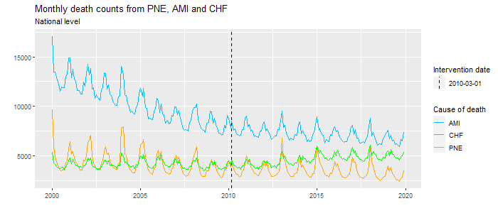
Figure 1: Monthly death counts from pneumonia, AMI and CHF at the national level. The dashed vertical bar indicates the intervention date.

At the national level, we find that the HRRP led to a medium and long-term increase in mortality from AMI. By comparing the national results with those emerging from the regional break down, we obtain interesting findings. Short-term mortality is concentrated in the first two regions for pneumonia. Interestingly, even though we did not find the presence of a short run effect for AMI at the national level, we can see mortality from AMI increased due to the HRRP in three regions (the null result in the South US might be behind the absence of a causal effect at the national level). For the mid-term effects, we can see that the increase in mortality from AMI is mostly driven by the Northeast, Midwest and West regions. Finally, the results from our long-term regional analysis show that the national result for AMI is mostly explained by the Northeast and West US regions. Finally, both the national and regional analyses reflected null effect estimates of the HRRP on CHF mortality.

As we see in Figure 2, the uncertainty bands for the cumulative effect estimates get wider as we predict further into the future. This is also true for the point-wise effect estimates (see Figure S.19). This is due to the auto-regressive mean structure which requires uncertainty quantification for outcomes further in the future to incorporate the uncertainty of parameters and imputed potential outcomes for all intermediate time periods. We find this to be an attractive property of this approach since it represents that the observed outcome time series trends are more trustworthy when extrapolating in the near future. For a fixed $k$, the width of the uncertainty band for our causal effect estimators will not go to zero, irrespective of the length of the pre-intervention period. That is because we estimate the causal effect for a single unit, we do not benefit from estimating averages over a sample, and as a result the uncertainty embedded in the posterior predictive distribution for the unit’s missing potential outcome will propagate to our estimator. Even though including predictors of the outcome could reduce the outcome model’s residual variance and as a result the variance of the imputed potential outcomes, the potential outcomes’ inherent variability will persist.

Table 2: Cumulative causal effect and $95\%$ credibility intervals of the HRRP on mortality from pneumonia, AMI and CHF at the national level. In this table, C$\Delta$ denotes the cumulative impact at the end of three different time horizons (short, mid, and long-term). Results with 95% CIs that do not include 0 are shown in bold.

PNE AMI CHF C$\Delta$ $2.5\%$ $97.5\%$ C$\Delta$ $2.5\%$ $97.5\%$ C$\Delta$ $2.5\%$ $97.5\%$ short-term 10,795 -2,092 23,665 12,333 -734 25,239 3,780 -3,035 10,509 mid-term 49,445 -36,549 134,641 83,970 3,555 162,972 35,300 -26,811 94,469 long-term 98,849 -149,887 340,540 223,041 2,647 442,617 94,727 -96,895 27,8605

Table 3: Causal effect of the HRRP on mortality across US regions. C$\Delta$ denotes the number of deaths attributed to the HRRP. C$\Delta^{p}$ shows the proportion of deaths attributed to the HRRP (and 95% credible intervals) in each region. Results are shown for the three time horizons: i) 1 year (December 2011); ii) 5 years (December 2015); iii) 9 years (December 2019). Bold face is used for estimates whose credible interval does not include zero.

PNE AMI CHF C$\Delta$ C$\Delta^{p}$ (95% CI) C$\Delta$ C$\Delta^{p}$  (95% CI) C$\Delta$ C$\Delta^{p}$  (95% CI) short-term Northeast 3,931 22.2 (5.6, 38.5) 3,541 10.7 (1.4, 20.1) 741 4.4 (-4.7, 13.2) Midwest 3,517 19.4 (1.4, 37.5) 3,644 08.9 (0.2, 17.5) 995 4.2 (-4.4, 12.7) South 3,669 13.5 (-2.4, 29.1) 3,394 5.3 (-2.3, 12.7) 582 1.7 (-5.8, 9.3) West 2,131 13.4 (-3.2, 30.1) 2,270 07.8 (0.9, 14.5) 1,319 8.7 (-0.1, 17.5) mid-term Northeast 16,155 28.9 (-5.4, 62.6) 20,294 20.3 (2, 38.7) 5,958 10.3 (-12.8, 32.8) Midwest 18,957 32.6 (-3.8, 69.4) 23,100 18.4 (1.2, 35.4) 10,157 12.5 (-10.6, 33.6) South 16,954 19.3 (-13.9, 51.8) 28,313 14.1 (-0.7, 28.9) 11,898 10.1 (-9.1, 28.9) West 14,247 27.7 (-8.2, 63.4) 18,404 20.2 (6.1, 34.7) 9,795 19.5 (-5.4, 43.1) long-term Northeast 31,269 34.2 (-28.5, 95.2) 52,046 33.5 (0.2, 65.6) 14,865 14.7 (-26.9, 55.6) Midwest 41,004 44.2 (-20.9, 110.7) 57,955 28.5 (-1.3, 58) 25,984 18.1 (-21.6, 56.6) South 35,671 24.8 (-33.8, 82.5) 77,855 23.4 (-2.6, 49.6) 32,349 15.5 (-18.1, 48.9) West 33,938 40.2 (-22.7, 102.8) 55,022 36.1 (10.8, 62.1) 27,003 28.6 (-14, 71.2)

Figure 2: Cumulative effect of the HRRP on mortality from pneumonia, AMI and CHF at the national and regional level for the intermediate time horizon ending in December 2015. Plots for the remaining regions are provided in the Online Resource.

3.4 Additional analyses of our data

Considering the policy importance of our results, we performed several checks to evaluate the performance of our approach and the robustness of our qualitative results to the model chosen and the methodology used. These checks correspond to analyses of the effect of the HRRP under the following general categories: (1) analyses based on our model and alternative choice of predictors, (2) analyses on control time series that are expected to be unaffected by the intervention, (3) analyses based on alternative methodologies that employ a different set of causal assumptions, and (4) analyses based on transformations of our data, The analyses are discussed in detail in Section E, and the acquired results are summarized here.

First, we evaluate the robustness of our quantitative results to alternative choices of predictor variables. We follow a three-step procedure: We establish alternative sets of predictor variables that one could consider. Then, for each set of predictors and without looking at the effect estimates based on each model, we inspect the posterior predictive checks of the model fits for each outcome and each set of covariates. If the check shows that the model is not a good fit for the observed data, the corresponding set of covariates is discarded. Using the models with predictors that passed the posterior predictive checks, we estimate the causal effects, and we compare them to the results from our original analysis. For our study, we considered three alternative sets of predictors: a) no predictors; b) all predictors excluding PM_2.5; and c) only weather covariates. The posterior predictive checks of the model without predictors (Figure S.5 in the Online Resource) show high residual autocorrelation, and therefore this model is discarded. Conversely, the model without PM_2.5 and the model with only the weather covariates fit the data well (see Figures S.9, S.9 and S.14, S.15 in the Online Resource). The causal effect estimates from these two models are shown in Table 4 and they are extremely similar to our original results in Table 2, illustrating that our results are robust to the choice of predictor variables.

Table 4: Cumulative causal effect and $95\%$ credibility intervals of the HRRP on mortality from pneumonia, AMI and CHF at the national level from two local linear trend models with different choices of regressors: (1) all regressors excluding PM_2.5; (2) only weather covariates.

PNE AMI CHF C$\Delta$ $2.5\%$ $97.5\%$ C$\Delta$ $2.5\%$ $97.5\%$ C$\Delta$ $2.5\%$ $97.5\%$ (1) short-term 10,756 -1,814 23,048 12,386 -372 25,274 3,432 -3,244 9,906 mid-term 47,828 -36,526 133,777 86,054 6,236 163,997 31,374 -32,046 91,649 long-term 98,180 -146,105 342,845 216,877 -5,393 437,220 91,494 -96,189 273,341 (2) short-term 10,555 -1,511 22,753 12,570 -583 25,396 3,709 -2,841 10,357 mid-term 48,263 -35,138 130,502 84,239 3,634 162,949 39,010 -20,062 95,792 long-term 105,614 -127,016 342,462 221,273 221 439,858 98,079 -84,724 274,474

As an additional robustness check, we performed falsification tests by repeating the analysis on death conditions that, in principle, should not be affected by the HRRP: if the estimated impact on such conditions is close to zero, we can be more confident on the results obtained for pneumonia, AMI, and CHF. To do so, we acquired monthly level death counts from the Centers for Disease Control and Prevention WONDER database by specifying as underlying cause of death the following codes: A00–B99 (infectious and parasitic diseases); C00–D49 (tumors); D50–D89 (diseases of the blood); F01–F99 (mental disorders); V00–Y99 (external causes of morbidity). Figure S.20 in the Online Resource shows the evolution in mortality from each disease from January 2000 to December 2019. We can observe an increasing trend in mortality from all causes in the considered period. The results from each estimated model are reported in Table 5 and show no evidence of a causal effect for any of the control outcomes. These results show that if unpredictable changes in mortality trends exist, they are not present in control conditions so we can be more reassured that such changes are also not present in the target conditions. In addition, falsification tests are also important to ascertain the impact of possible co-occurring policies: if no evidence of an effect is found on control conditions, we can be more confident that co-occurring policies had no impact on target conditions as well. Finally, we verified the absence of anticipatory effects on both the true outcomes and on control conditions (see Table S.1 in the Online Resources).

Table 5: Falsification tests. Cumulative causal effect of the HRRP on control outcomes at three different time horizons.

Short term Mid term Long term C$\Delta$ 2.5% 97.5% C$\Delta$ 2.5% 97.5% C$\Delta$ 2.5% 97.5% Infections 3,147 -2,808 9,131 20,725 -33,304 76,348 44,187 -126,529 217,690 Tumors 6,548 -3,068 16,106 57,050 -16,135 127,480 160,398 -40,405 361,319 Blood diseases 1,371 -1,868 4,565 9,457 -33,576 53,331 18,490 -140,143 172,038 Mental disorders 12,072 -854 24,870 5,739 -78,555 87,538 -221,402 -506,026 24,146 External causes 5,673 -578 11,833 41,207 -27,218 109,316 117,288 -108,225 344,842

As we discussed in Section 2.4, our approach can suffer if there exist structural changes in the temporal trends of the outcome time series after the intervention that are not due to the intervention. To evaluate the robustness of our qualitative analyses, we considered alternative methodologies that aim to address these issues, namely: interrupted time series, difference-in-differences (DiD) and synthetic control methods. For the synthetic control approach, we employed the augmented synthetic control approach of Ben-Michael et al. (2021) using mortality from conditions not targeted by the HRRP as control time series, in line with Gaughan et al. (2019). We include a detailed discussion of these methods and corresponding results in Section E of the Online Resource. All these approaches rely on underlying assumptions that should be carefully addressed in a complete causal analysis. We find that results based on the ITS approaches in Miratrix et al. (2019), as well results based on synthetic control methods yield results which are in line in direction and magnitude with the ones shown in Table 2.

In our main analyses, we used Gaussian models for our mortality counts because our interest is in estimating the number of deaths that were avoided by or attributed to the HRRP. We have found that Poisson regression models with autoregressive mean structure do not perform well in predicting future outcomes due to high uncertainty (Wheeler, 2018). We found that our Gaussian model fit the observed data well even though these are count data. As a companion analysis, we considered alternative model specifications for both the true and the control outcomes, namely, a Gaussian Bayesian time series model estimated on the logarithmic transformation of the monthly death counts and a Gaussian Bayesian time series model estimated on the logit transformation of the monthly death rate from each condition. The results are reported in the Online Resource and seem to exclude the presence of causal effects. However, in Section E we show that such models target different causal effect estimands: a multiplicative effect on the outcome for the log-normal model, a causal effect on the log-odds ratio for the logit transformation. Thus, such results seem to suggest that the HRRP policy incentive scheme had an additive effect on the death counts from pneumonia and AMI, as shown in Table 2.

4 Discussion

We find that the main methodological contributions of this paper are three-fold. In a time-series setting with one time series and one interventional time point, we (1) defined quantities to be estimated in terms of potential outcomes, (2) formalized the assumptions on which a previously-developed (Brodersen et al., 2015) Bayesian time series model was based (which had not been done until now), and importantly (3) provided a comprehensive interrogation of the assumptions underlying the estimation of such causal estimands in the context of our study, laying the foundation for the use of this method in a wide range of applications assessing clinical outcomes for health policy in non-randomized settings.

In our illustrative study, we evaluated the effect of the HRRP passage on mortality among the elderly. One of the key difference of our approach compared to previous associational studies is our focus on the whole region of interest as one unit measured over time, which allows us to estimate the effect of the HRRP passage on the whole population it meant to serve. Since the presented approach bypasses some complicating aspects of policy evaluation, we view our approach as complementary to approaches that compare penalized to non-penalized hospitals.

To our knowledge, this is the first paper evaluating the causal effect of the HRRP. Previously published analyses have suggested that after enactment of the HRRP, readmissions have decreased for all of the 3 initial penalty conditions (Zuckerman et al., 2016; Desai et al., 2016; Wasfy et al., 2017), even though these reductions in readmissions are likely due to increases in post-discharge emergency department visits or observation stays (Wadhera et al., 2019). Although our results are not directly comparable to the above studies, a fraction of reduced readmissions may result in increased mortality; in addition, our analysis is also able to capture the portion of mortality due to the HRRP arising from other sources (e.g., delayed first admissions and in-hospital mortality), or due to the possibility that hospital resources were redistributed away from reducing mortality to reducing readmissions.

Even though reductions in readmissions are encouraging, our analysis raises concerns about increased mortality caused by the HRRP. From the perspective of policy evaluation, our results illustrate that the future of the HRRP might have to be reassessed and future amendments might be necessary to avoid a detrimental impact of the policy on the population it was meant to serve.

Declarations

Funding

Funding was provided by National Institutes of Health R01 GM111339, R01 ES024332, R01 ES026217, P50MD010428, DP2MD012722, R01 ES028033, USEPA 83615601, and Health Effects Institute 4953-RFA14-3/16-4. The contents of this work are solely the responsibility of the grantee and do not necessarily represent the official views of the USEPA. Further, USEPA does not endorse the purchase of any commercial products or services mentioned in the publication. Research described in this article was conducted under contract to the Health Effects Institute (HEI), an organization jointly funded by the United States Environmental Protection Agency (EPA) (Assistance Award No.CR-83467701) and certain motor vehicle and engine manufacturers. The contents of this article do not necessarily reflect the views of HEI, or its sponsors, nor do they necessarily reflect the views and policies of the EPA or motor vehicle and engine manufacturers. Dr. Wasfy is supported by National Institutes of Health and Harvard Catalyst KL2 TR001100 and American Heart Association 18CDA34110215.

Dr. Menchetti and Prof. Mealli thank the Department of Excellence 2018-2022 funding provided by the Italian Ministry of Education, University and Research (MIUR).

The authors have no conflicts of interest to declare that are relevant to the content of this article.

Supporting information for the manuscript
Evaluating Federal Policies Using Bayesian Time Series Models: Estimating the Causal Impact of the Hospital Readmissions Reduction Program
by
Georgia PapadogeorgouEqually contributing authors University of Florida, Department of Statistics, Gainesville, FL, USA. ORCID 0000-0002-1982-2245. Corresponding Author. gpapadogeorgou@ufl.edu.,   Fiammetta Menchetti^*University of Florence, DiSIA and Florence Center for Data Science, Florence, Italy. ORCID 0000-0003-3463-0206. ,   Christine ChoiratSwiss Data Science Center, ETH Zürich and EPFL, Lausanne & Institute of Global Health, Faculty of medicine, University of Geneva, Switzerland. ,
Jason H. Wasfy Cardiology Division, Department of Medicine, Massachusetts General Hospital, Harvard Medical School, Boston, MA, USA,   Corwin M. ZiglerUniversity of Texas at Austin, Department of Statistics and Data Science, Department of Women’s Health, Austin, TX, USA,   Fabrizia MealliUniversity of Florence, DiSIA and Florence Center for Data Science, and European University Institute, Department of Economics, Florence, Italy. ORCID 0000-0002-1076-9249

A Census regions and divisions of the United States

The regional data gathered from the WONDER database follow the region definition of the Census Bureau. We report below the map and the list of states belonging to each region, as downloaded from the website https://www2.census.gov/geo/pdfs/maps-data/maps/reference/us_regdiv.pdf (Retrieved November 19, 2021).

B Investigating patterns in our data

We first investigated seasonality in our data, which is evident from Figure S.1 showing the autocorrelation plots for each outcome at the national level: the spikes every 12 lags indicate yearly seasonality. The seasonality patterns are also evident from Figure 1 in the main paper and from Figure S.2 below, where we also notice a decreasing trend in mortality from pneumonia and AMI both at the national and regional level. Finally, Figure S.3 shows the evolution of covariates during the analysis period. There, we see that the poverty levels show a change in their trend in the pre- and in the post-intervention period.

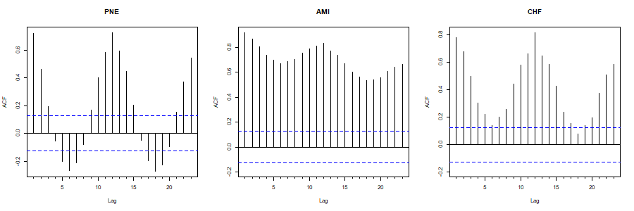
Figure S.1: Autocorrelation functions of the three outcome variables (death counts from pneumonia, AMI and CHF) at the national level. All plots show spikes every $12$ lags, indicating a clear seasonal pattern.

Figure S.2: Monthly death counts from pneumonia (panel A), AMI (panel B) and CHF (panel C), by census region. The dashed vertical bar indicates the intervention date and the four census regions are coded as follows: Northeast, Midwest, South, West.

A)
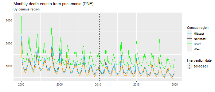
B)
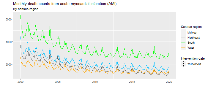
C)

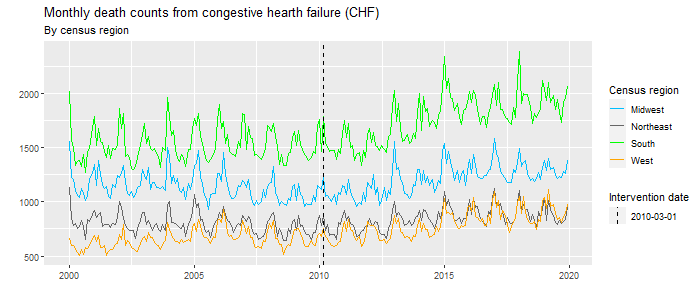
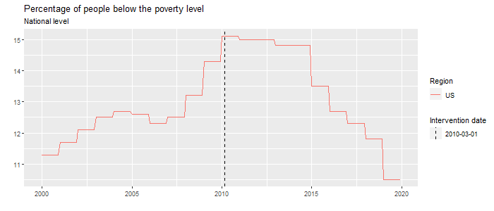
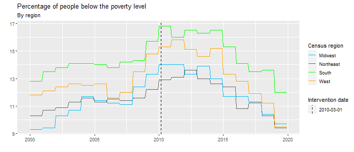
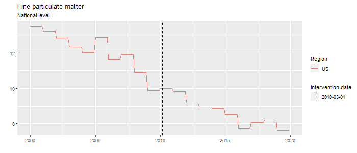
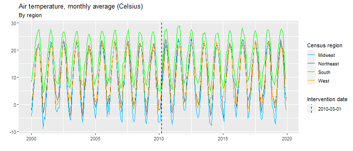
Figure S.3: Evolution of the covariates during the analysis period. Starting from top: i) percentage of people below the poverty level; ii) percentage of people below the poverty level by region; ii) concentration of fine particulate matter (yearly average, $\mu g/m^{3}$); air temperature (monthly average, ${}^{\circ}C$) by region.

C Investigating model fit in the pre-intervention period

In Section 2.5 we assert that even though Assumption 2 can not be formally tested, we can still check whether the model fits well to the pre-intervention data: if it doesn’t, it is unlikely that the assumed model adequately describes post-treatment outcomes in the absence of the intervention. To this aim, we employ posterior predictive checks, we assess model convergence and, since we include regressors, we check posterior inclusion probabilities to see whether they help predicting the outcome in the pre-intervention period.

C.1 Posterior predictive checks

As described earlier, we use posterior predictive checks to inspect the model fit to pre-intervention data. The results from the posterior predictive checks for each model are shown as:

• Figure S.5: selected model with local linear trend, seasonality, and all predictors.

• Figure S.5: model with local linear trend, seasonality,, and no predictors.

• Figure S.7: model with local trend, seasonality, and no predictors.

• Figure S.7: model with local trend, seasonality, and all predictors.

• Figure S.9: model with local linear trend, seasonality, and all predictors excluding PM_2.5.

• Figure S.9: model with local linear trend, seasonality, and only weather-related predictors.

We notice that the models without regressors exhibit excess residuals autocorrelation (Figures S.5 and S.7). The local level model with the addition of regressors shows better fit to pre-intervention data than the model without (Figure S.7) but it still has slightly larger residuals autocorrelations compared to the selected model. The posterior predictive checks that better align to those of the selected model are shown in Figures S.9 and S.9, corresponding to the local linear trend and seasonal models with only a subset of regressors.

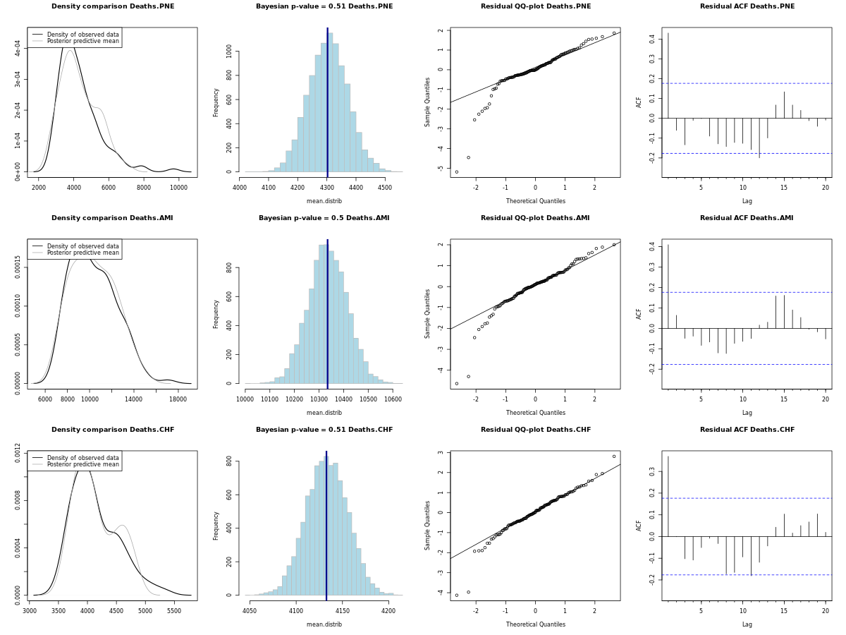
Figure S.4: Posterior predictive checks for the selected local linear trend and seasonal models estimated in the pre-intervention period on the death counts from each condition (PNE, AMI and CHF) at the national level.

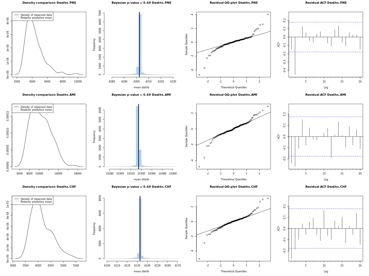
Figure S.5: Posterior predictive checks for a local linear trend and seasonal model with no regressors estimated in the pre-intervention period on the death counts from each condition.

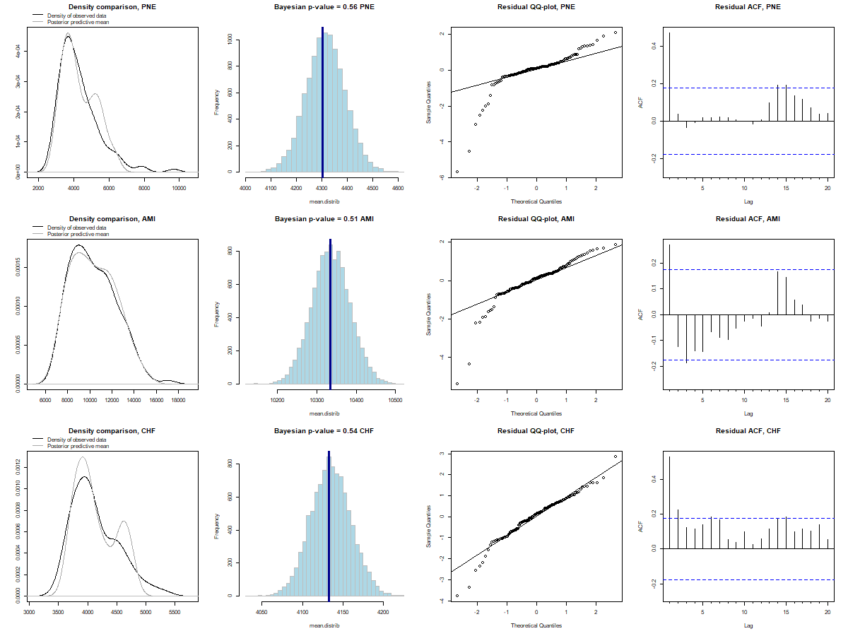
Figure S.6: Posterior predictive checks for a local level and seasonal model with no regressors estimated in the pre-intervention period on the death counts from each condition.

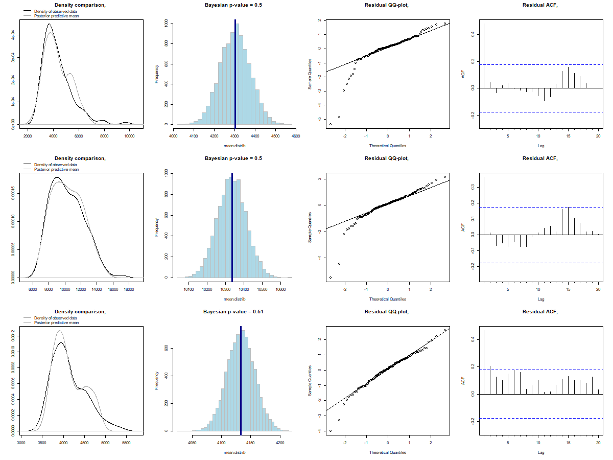
Figure S.7: Posterior predictive checks for a local level and seasonal model with regressors estimated in the pre-intervention period on the death counts from each condition.

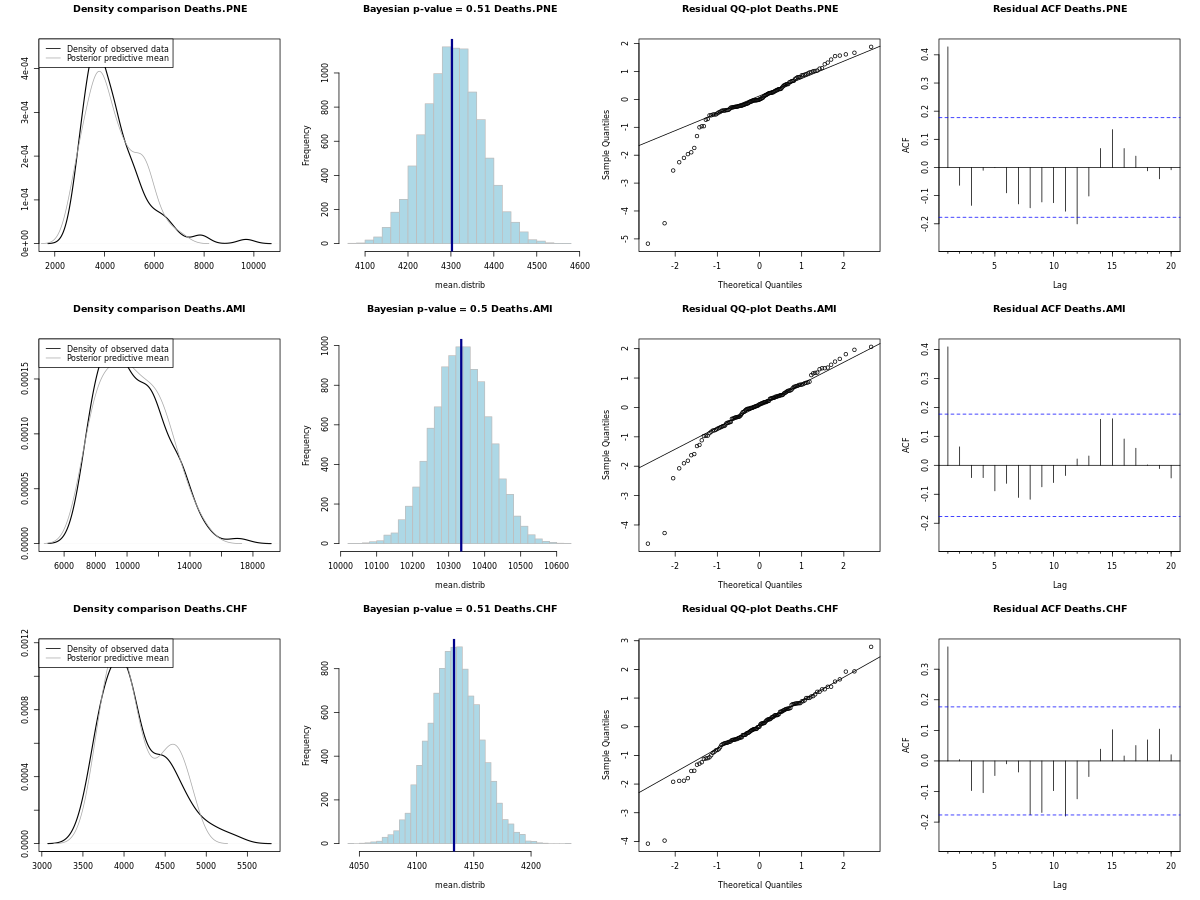
Figure S.8: Posterior predictive checks for a local linear trend and seasonal model excluding PM_2.5 from the set of regressors.

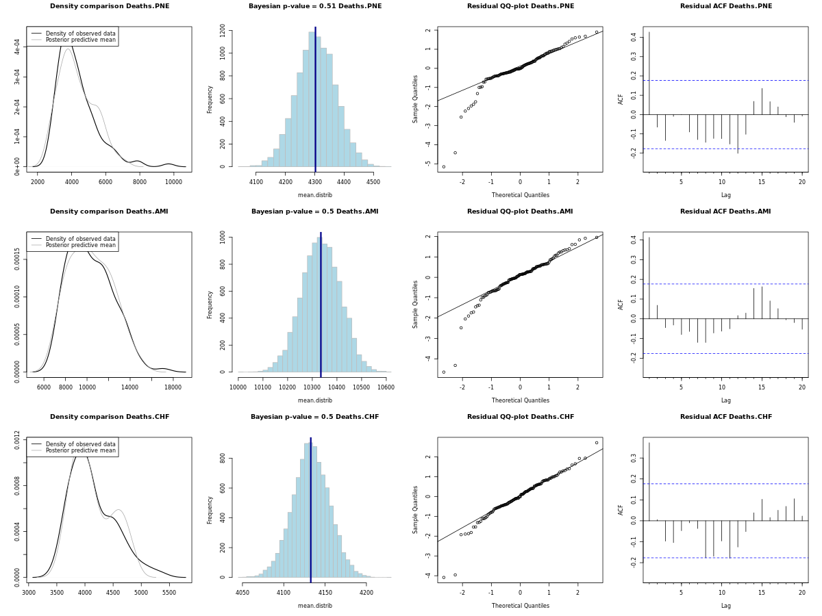
Figure S.9: Posterior predictive checks for a local linear trend and seasonal model having as regressors the weather covariates only.

C.2 MCMC convergence

We investigated trace plots of identifiable parameters to visually inspect the convergence of the Markov chain to the stationary distribution. Figures S.10 – S.15 show the trace plots of the alternative models that we tested in the same order as in Section C.1.

We notice that the local level models have convergency issues in the variance of the seasonal component (Figures S.12 and S.14). Instead, the selected local linear and seasonal model seems to converge to the stationary distribution. The models for which the MCMC showed lack of convergence were not used to evaluate the causal effect.

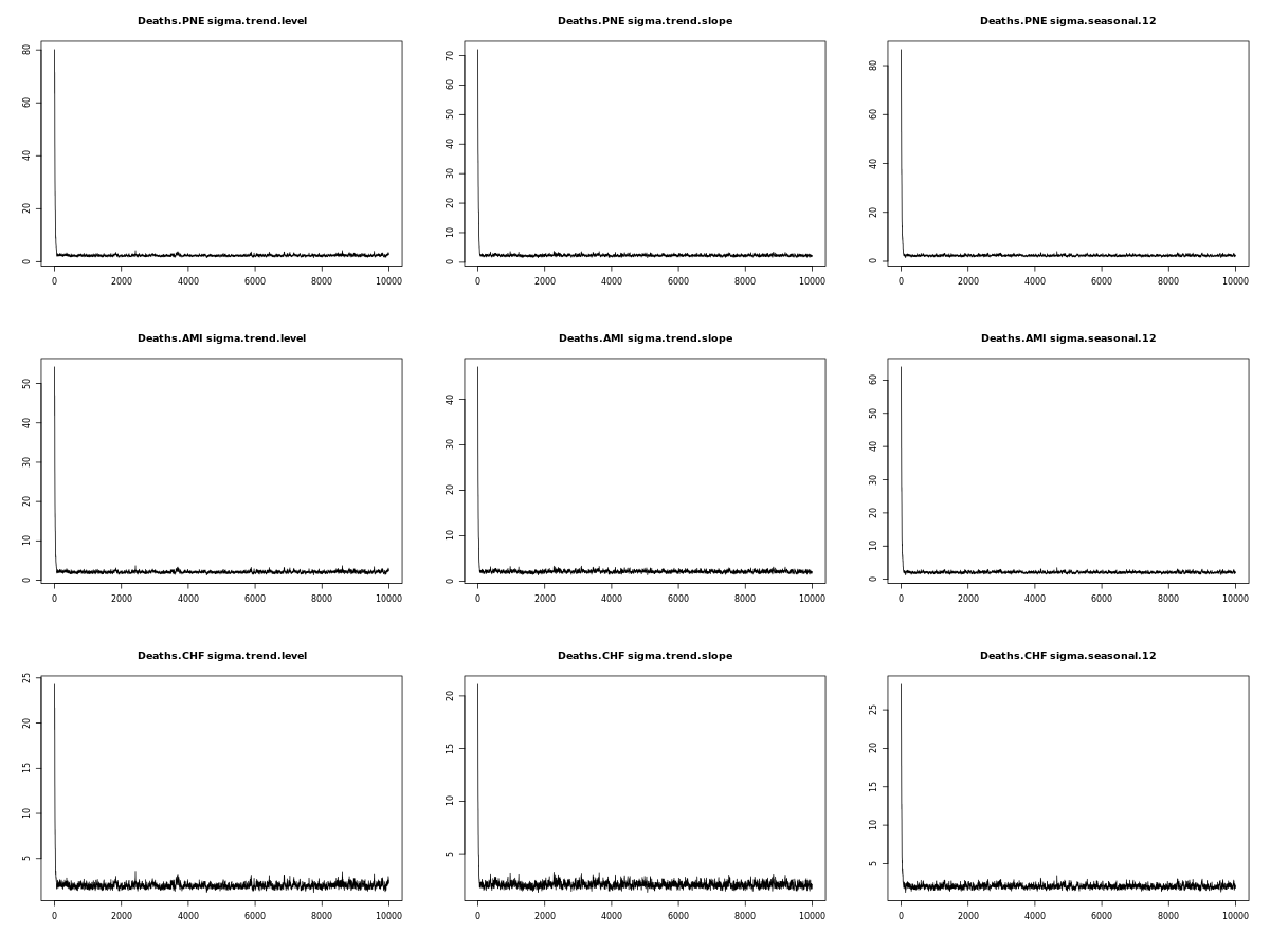
Figure S.10: Trace plots for the selected local linear and seasonal model estimated in the pre-intervention period on the death counts from each condition (PNE, AMI and CHF) at the national level.

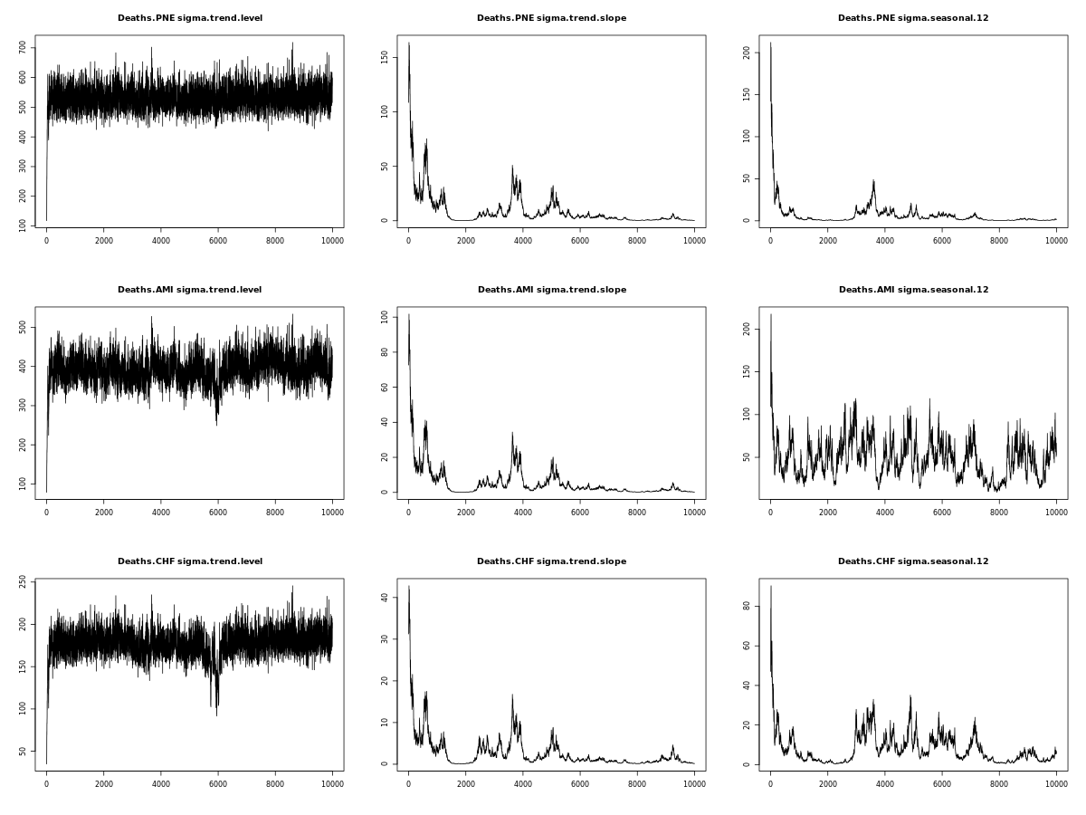
Figure S.11: Trace plots for the alternative local linear and seasonal model without regressors estimated in the pre-intervention period on the death counts from each condition.

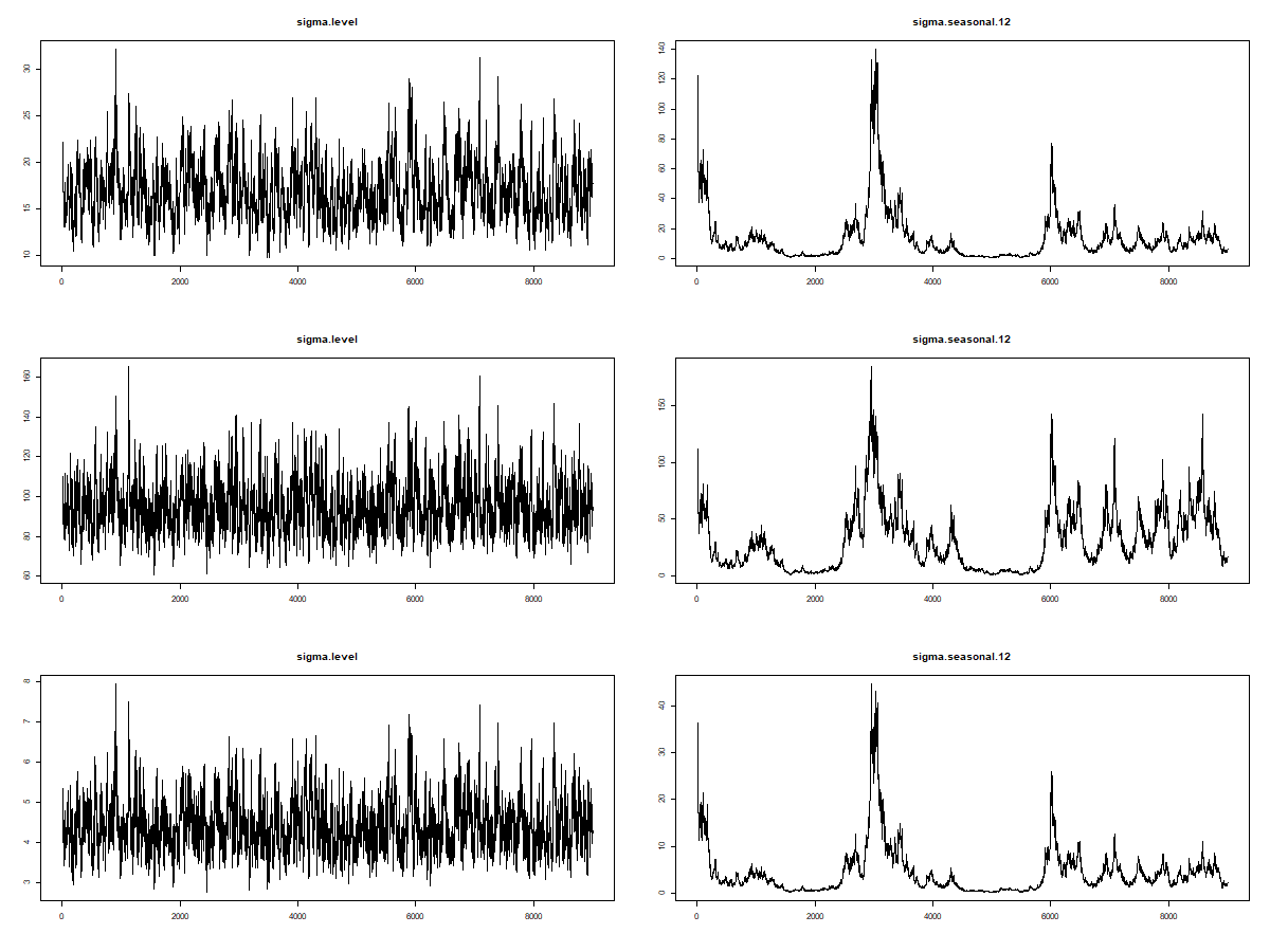
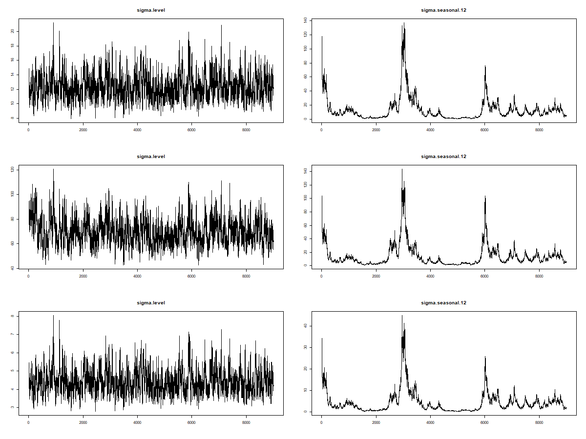
Figure S.12: Trace plots for the alternative local level and seasonal model without regressors estimated in the pre-intervention period on the death counts from each condition.

Figure S.13: Trace plots for the alternative local level and seasonal model with regressors estimated in the pre-intervention period on the death counts from each condition.

Figure S.14: Trace plots for a local linear trend and seasonal model excluding PM_2.5 from the set of regressors.

Figure S.15: Trace plots for a local linear trend and seasonal model having as regressors the weather covariates only.

C.3 Posterior inclusion probabilities

The prior distribution on the regression coefficients $\beta$ is a spike-and-slab prior defined after a data augmentation step where we add a selection vector whose components can either be 0 (the corresponding regressor is deleted from the model) or 1 (the corresponding regressor is included in the model). At each MCMC iteration, a stochastic search variable selection is performed: the Gibbs sampling algorithm inspects all possible models by changing the selection vector component-wise, so that, at each iteration, only the most likely model is retained. By averaging across all selected models (one for each MCMC iteration) we obtain the posterior inclusion probabilities for each regressor. These are useful to understand whether the covariates that we choose are related to the outcome and which ones retain most of the information to improve the prediction of the outcome in the pre-intervention period.

Figure S.16 shows the results for the national analyses. We notice that temperature information seems to play a crucial role in modeling deaths from all conditions at the national level, followed by poverty. This evidence is supported by the regional analyses as well, results of which are shown in Figure S.17. Interestingly, from the regional breakdown we observe that poverty is linked to death counts especially in the South and West regions (its posterior inclusion probability in the model for CHF is 60% in the South and exceeds 80% in the West).

Figure S.16: Posterior inclusion probabilities of the covariates included in the selected local linear and seasonal models estimated in the pre-intervention period on the death counts from each condition at the national level.

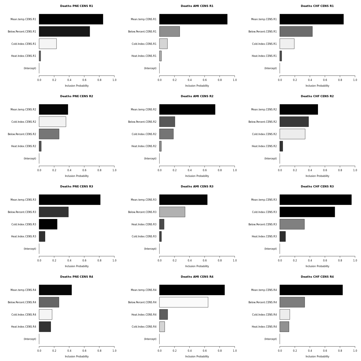
Figure S.17: Posterior inclusion probabilities of the covariates included in the selected local linear and seasonal models estimated in the pre-intervention period on the death counts from each condition, by region.

D Additional plots of the estimated causal effects

We now display additional plots of the estimated causal effects. Figure S.18 provides a visual overview of the mid-term cumulative impacts generated by the HRRP on mortality for the remaining regions (Midwest, South, West). In addition, Figure S.19 shows the comparison between the observed series and the predicted outcome based on the model fitted to the pre-intervention data. We notice that the fitted values before the intervention are very close to the observed values, which is a further indicator of model adequacy. Therefore, based on Assumption 2, we can attribute the deviation from the observed series in the post-intervention period to the HRRP (the deviation is also visible in the Figure).

Figure S.18: Cumulative effect of the HRRP on mortality from pneumonia, AMI and CHF for the remaining regions at the intermediate time horizon ending in December 2015.

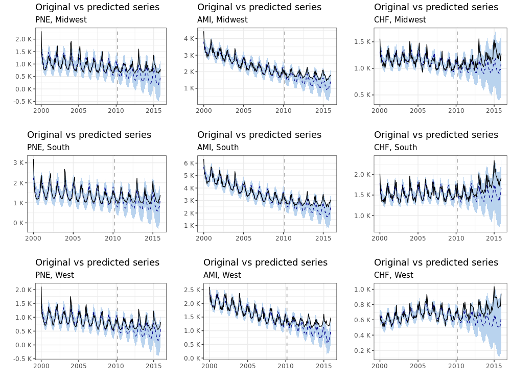
Figure S.19: Comparison of the observed series with the predicted outcome from the selected local linear and seasonal model at the intermediate time horizon ending in December 2015, by region.

E Robustness checks

Conscious of the policy implication of our findings, we run several checks to see if the results are robust to different model specifications. We run additional analyses with different model specifications and using alternative methods that are commonly used in causal inference literature. The next sections summarize the main results.

E.1 Alternative choice of predictors

First of all, we performed a sensitivity analysis aimed at assessing if and how much the estimates depend on different choices of predictors. The results are reported in Section 3.3 of the main paper and show that the empirical findings for pneumonia, AMI and CHF are consistent across different sets of regressors. Diagnostic tests were shown in Section C.

E.2 Falsification tests

We run falsification tests by repeating the analyses on control outcomes that, in principle, should be unaffected by the HRRP incentive scheme. Figure S.20 displays the evolution of the control outcomes over the analysis period. Under the usual model specification (local linear trend and seasonal model estimated on count data) no causal effect is found on control outcomes (see Table 5 in the main paper). We also considered whether the control conditions indicated an anticipatory effect by fictionally setting the treatment initiation period as three months earlier and using our method to evaluate the effect in the three month time period that follows. In Table S.1, we see that none of the control conditions (or the target conditions) shows an anticipatory effect.

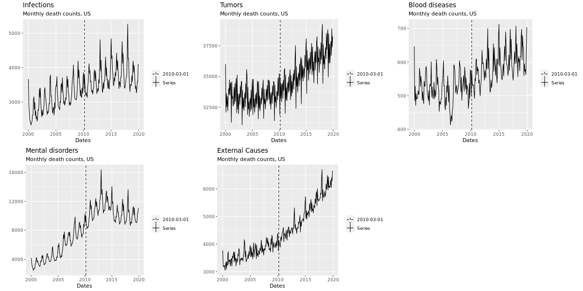
Figure S.20: Evolution over time of the control outcomes at the US level. The dashed vertical bar indicates the date when the HRRP was introduced.

Table S.1: Anticipation effects of the HRRP on the falsification outcomes up to 3 months before the intervention.

	C$\Delta$	2.5%	97.5%
Infections	-685	-1,362	52
Tumors	952	-1,113	2,881
Blood diseases	-55	-210	99
Mental disorders	1,143	-1,655	4,219
External causes	-11	-578	558
Pneumonia	-1,323	-4,112	1,329
AMI	-1,344	-3997	1,338
CHF	579	-390	1,451

E.3 Interrupted time series approach

Table S.2: Estimated post-intervention slope change in a segmented regression for pneumonia, AMI and CHF at three different time horizons. Significant results at the $5$% level are shown in bold.

	PNE				AMI				CHF
	$\beta_{3}$	Std. Error	t stat		$\beta_{3}$	Std. Error	t stat		$\beta_{3}$	Std. Error	t stat
Short-term	6.94	18.80	0.37		29.02	15.29	1.90		-2.80	6.51	-0.43
Mid-term	12.24	5.57	2.20		43.49	4.52	9.62		12.48	2.11	5.92
Long-term	14.09	4.86	2.90		46.39	3.96	11.71		12.32	2.06	5.98

For comparison purposes, we repeated the analysis using the Interrupted Time Series (ITS) approach. The usual ITS design applies when there are policy changes affecting all units simultaneously. Such design would then be a very natural choice in our setting, since the HRRP has the characteristics of an extensive policy affecting all hospitals and patients at the same time. Segmented regression is the simplest form of ITS analysis and involves estimating a model as the following [Wagner et al., 2002, Bernal et al., 2017],

$$Y_{t}=\beta_{0}+\beta_{1}t+\beta_{2}D_{t}+\beta_{3}tD_{t}+\epsilon_{t}$$ (S.1)

where: $t$ is the time since the start of the study; $D_{t}$ is an indicator variable coded $0$ before the intervention and $0$ after the intervention; $tD_{t}$ is the interaction between the indicator variable and the time and counts the time points after the intervention (it is $0$ before the policy introduction); $\epsilon_{t}\sim i.i.dN(0,\sigma^{2})$ denote the error terms, which are typically assumed to be uncorrelated, homoschedastic and independent. Thus, under such formulation, $\beta_{0}$ and $\beta_{1}$ would capture, respectively, the baseline level and trend; $\beta_{2}$ estimates the level change after the intervention and $\beta_{3}$ estimates the change in trend. Model equation (S.1) can then be adapted to the characteristics of the data. For example, in our case we also added covariates reflecting the presence of possible confounders linked to the treatment and the outcome and seasonality effects (captured by the inclusion of dummy variables). The results are reported in Table S.2. For brevity reasons, the table only shows the coefficient estimates for $\beta_{3}$, since the estimates for the level change, $\beta_{2}$, was never significant at the $5$% level. Results seem to support the idea that mortality trend increased after the HRRP both in the mid-term and in the long-term for all conditions. We also used these models to predict the outcome had the intervention not taken place by setting the corresponding treatment indicator to 0. We used these predicted outcomes to acquire estimates of $C\Delta_{K}$ for the short-, mid-, and long-term. These results are shown in Table S.3, though it is not clear how one could acquire valid confidence intervals for these quantities based on this model. We see that the magnitude of the effect estimates based on the ITS analyses is comparable to the magnitude of the results based on our method.

Table S.3: Cumulative effect estimates for pneumonia, AMI and CHF at three different time horizons based on the ITS analysis.

	pneumonia	AMI	CHF
Short-term	2,738	15,445	747
Mid-term	36,199	126,074	27,356
Long-term	101,941	347,064	77,266

However, segmented regression models do not typically account for autocorrelation. To incorporate that, we should allow the error term to follow an ARIMA process, as it is recommended in Schaffer et al. [2021]. In addition, seasonality can also be formally handled by differencing, i.e., calculating the difference between adjacent observations (for a detailed review of ARIMA models, see Brockwell and Davis [2009]). By applying this less trivial ITS approach to our data we obtain a significant increase in mortality trends for pneumonia and CHF. The results are reported in Table S.4.

Table S.4: Estimated post-intervention slope change in an ITS regression with ARIMA errors for pneumonia, AMI and CHF at three different time horizons. Significant results at the $5$% level are shown in bold.

	PNE				AMI				CHF
	$\beta_{3}$	Std. Error	t stat		$\beta_{3}$	Std. Error	t stat		$\beta_{3}$	Std. Error	t stat
Short-term	3.68	16.41	0.22		29.41	17.25	1.70		3.35	7.01	0.48
Mid-term	12.97	6.28	2.06		25.99	14.18	1.83		12.87	2.42	5.32
Long-term	13.34	5.95	2.24		31.55	17.26	1.83		10.94	2.30	4.75

Both segmented regression models and ITS models with ARIMA errors are estimated on the full pre-intervention and post-intervention data, which implies that one must postulate a specific structure on the effect, e.g., a pulse, a step change, a transient change. For example, results above have been obtained under the assumption that the HRRP produced a “ramp” effect on the outcome, i.e., a change in slope that occurs after the intervention [Schaffer et al., 2021]. However, if this assumption is wrong, the estimated effect will necessarily be biased. In addition, to produce effect estimates at different point in time, model estimation has to be repeated multiple times adjusting the length of the time series, which is time consuming and sub-optimal (the estimated coefficient is an average over the period). A few recent approaches overcome this limitation [Miratrix et al., 2019, Menchetti et al., 2021]. In particular, Miratrix et al. [2019] propose a straightforward generalization of ITS designs by performing model estimation up to the intervention time point and then simulate different outcome trajectories from the theoretical distributions of estimated model parameters. In this way, no structure is imposed on the causal effect.

We therefore use the ITS approach proposed by Miratrix et al. [2019] to estimate the causal effect of the HRRP on mortality from pneumonia, AMI and CHF. The results are reported in Table S.5 and are analogous to those reported in the paper obtained with the Bayesian structural time series approach. All the estimates have been obtained with the simITS R package [Miratrix, 2020].

Table S.5: Cumulative causal effect and $95\%$ credibility intervals of the HRRP on mortality from pneumonia, AMI and CHF at the national level estimated with the ITS approach of Miratrix et al. [2019]. In this table, C$\Delta$ denotes the cumulative impact at the end of three different time horizons (short, mid, and long-term). Results with 95% CIs that do not include 0 are shown in bold.

	PNE				AMI				CHF
	C$\Delta$	2.5%	97.5%		C$\Delta$	2.5%	97.5%		C$\Delta$	2.5%	97.5%
Short-term	-4,929	-30,035	18,339		9,329	-16,313	32,127		-3,956	-13,891	5,096
Mid-term	-900	-83,367	75,484		94,515	17,271	168,923		14,311	-16,547	44,342
Long-term	1,901	-166,226	157,712		261,164	101,582	414,572		51,096	-13,740	109,168

E.4 Difference-in-Differences

A widely adopted method to evaluate the impact of an intervention on time series data is Difference-in-Difference (DiD) (see e.g., Card and Krueger [1993], Meyer et al. [1995], Angrist and Pischke [2008]). In its simplest formulation, this method requires to observe a treated and a control group at a single point in time before and after the intervention; the effect is then estimated by contrasting the change in the average outcome for the treated group with that of the control group. However, DiD often relies on the assumption that, in the absence of treatment, the outcomes of the treated and control units would have followed parallel paths. Therefore, before using DiD for the purpose of a causal analysis, it is generally recommended to check whether pre-intervention trends of the treated and control outcomes are parallel [Ryan et al., 2015, O’Neill et al., 2016].

In our case, we attempted to use the DiD approach taking as control conditions the control outcomes analysed in Section E.2, since we found that mortality from such conditions was unaffected by the HRRP. We therefore checked the validity of the parallel trend assumption by plotting the pre-intervention mortality trends from our outcomes and the control outcomes. As we can see from Figure S.21, the pre-intervention trends of the control conditions are not parallel to those exhibited by pneumonia, AMI and CHF. For this reason, we do not recommend to adopt DiD in our specific setting.

Figure S.21: Pre-intervention trends of pneumonia, AMI and CHF compared to that of possible control conditions. To ease comparison by correcting for different scales, death counts are scaled by their starting values in January 2000 (base month). Blue is used for the target condition, and black for the average of the control conditions.

Monthly death counts in the pre-intervention period

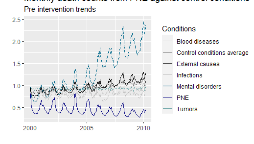
(a) PNE

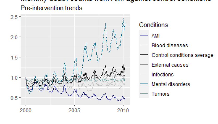
(b) AMI

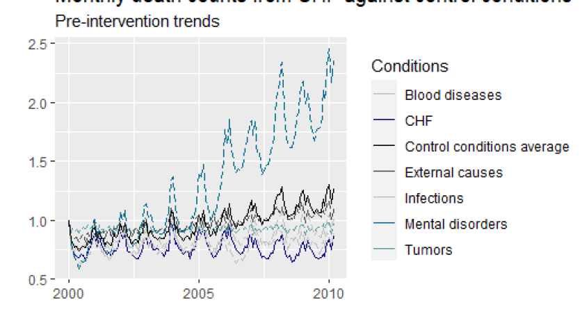
(c) CHF

E.5 Synthetic control methodology

An alternative approach that does not rely on the parallel trend assumption is the synthetic control method [Abadie and Gardeazabal, 2003, Abadie et al., 2010, 2015], which, instead, creates a synthetic time series by taking a weighted average of control series in a “donor pool” that are unaffected by the intervention. The weights are found by minimizing the distance between pre-treatment outcomes and the synthetic time series. The weights are usually restricted to be non-negative (non-negativity) and to sum up to 1 (adding-up) but several generalizations have been recently introduced. Indeed, relaxing these restrictions may be useful when the outcome of interest is an outlier with respect to the other units and in case of negative correlations between the outcome and the control series, thereby increasing prediction accuracy in the post-intervention period [Doudchenko and Imbens, 2016].

We therefore adopt the augmented synthetic control method proposed in Ben-Michael et al. [2021], which relaxes both the adding-up and the non-negativity restrictions and augments the common synthetic control approach with an outcome model that allows to remove the bias due to an imperfect pre-treatment fit. This method also permits to include auxiliary covariates by directly including them into the balance objective for the synthetic control method, as it is done for the controls. We use time series from conditions that are not expected to be impacted by the intervention as the control pool, similarly to Gaughan et al. [2019]. All the estimates have been obtained using the augsynth R package. Figure S.22 plots the estimated causal effect of the HRRP on each condition. The estimated cumulative effects $C\Delta_{k}$ in the short, medium and long run are reported in Table S.6 and have been obtained by adding up the impact estimates at each point in time after the intervention. Although it remains unclear how to obtain valid confidence intervals for these estimates, we can notice, once again, that their magnitude is aligned with the results reported in Table 2 under the selected Bayesian structural time series approach, though again slightly larger.

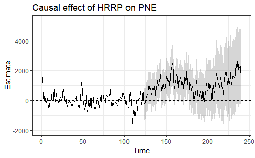
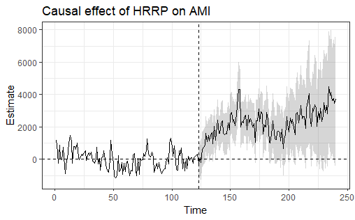
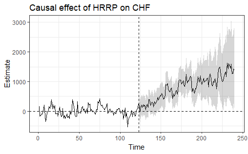
Figure S.22: Estimated pointwise causal effects of HRRP under the augmented synthetic control method.

Table S.6: Cumulative effect estimates for pneumonia, AMI and CHF at three different time horizons based on the augmented synthetic control analysis.

	pneumonia	AMI	CHF
short-run	15,286	27,972	4,626
mid-run	68,349	134,961	41,120
long-run	126,547	265,566	96,580

E.6 Alternative model specifications based on transformations of our outcome variable

Referring to the main model with local linear trend, seasonality and predictors as “Model 1”, we also tested alternative model specifications, namely:

1. Gaussian Bayesian structural time series model estimated on the logarithmic transformation of the monthly death counts (Model 2);

2. Gaussian Bayesian structural time series model estimated on the logit transformation of the monthly death rate from each alternative condition, i.e., monthly death counts divided by the over 65 population (Model 3).

All the tested models include covariates. The posterior predictive checks and MCMC diagnostics for Model 1 on the target conditions are inspected in Sections C.1 and C.2, respectively. Figure S.23 shows the posterior predictive checks for Model 1 on the control conditions, Figures S.24 and S.25 show the posterior predictive checks for Model 2 for the target and control conditions respectively, and Figures S.26 and S.27 show the same quantities based on Model 3. Figures S.28–S.32 show the MCMC convergence checks for the models in the same order. We see that all models converged and seem to provide a good fit to the pre-intervention data. Residuals diagnostics are also good, with a slightly better Normal approximation for Model 1, whereas the worst approximation seems to be under Model 3 (see for example the Normal QQ plots for the external causes and blood diseases under Model 3 compared to Model 1). This might be explained by the different frequency for the numerator (monthly death counts) and the denominator (yearly population estimates) that are used to compute mortality rates.

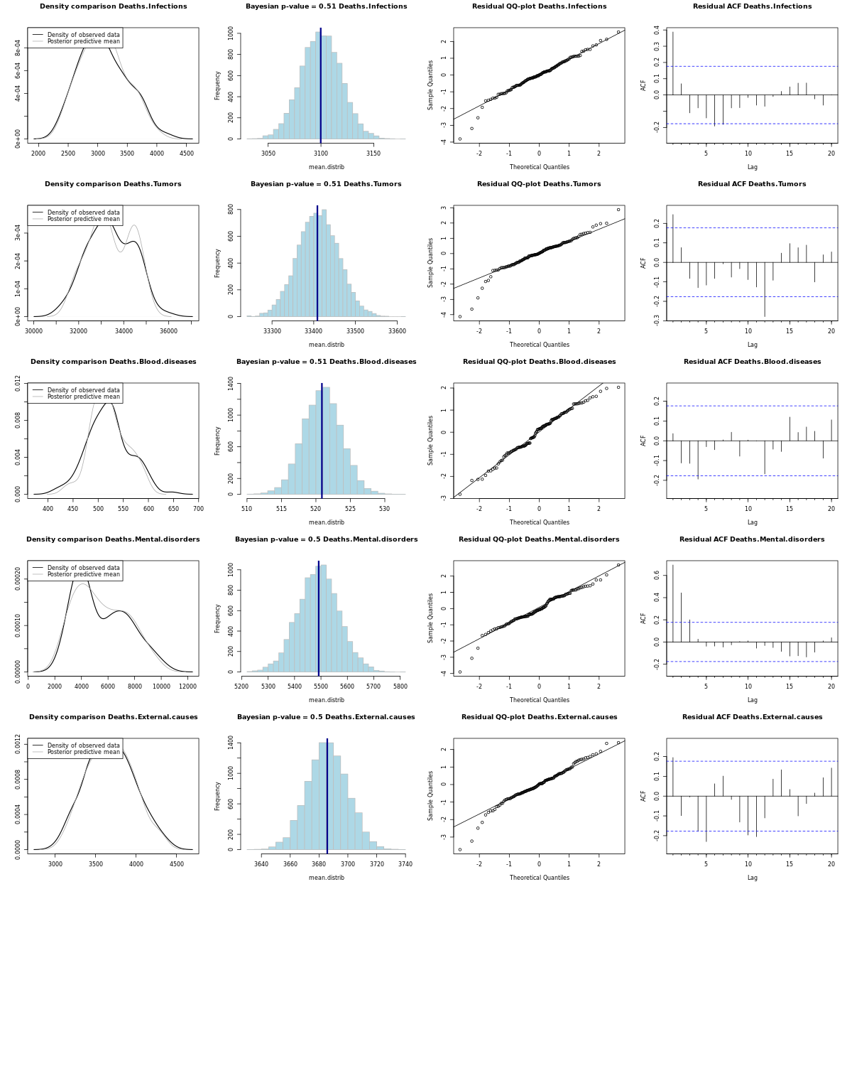
Figure S.23: Posterior predictive checks of control outcomes under Model 1.

Figure S.24: Posterior predictive checks for pneumonia, AMI and CHF under Model 2.

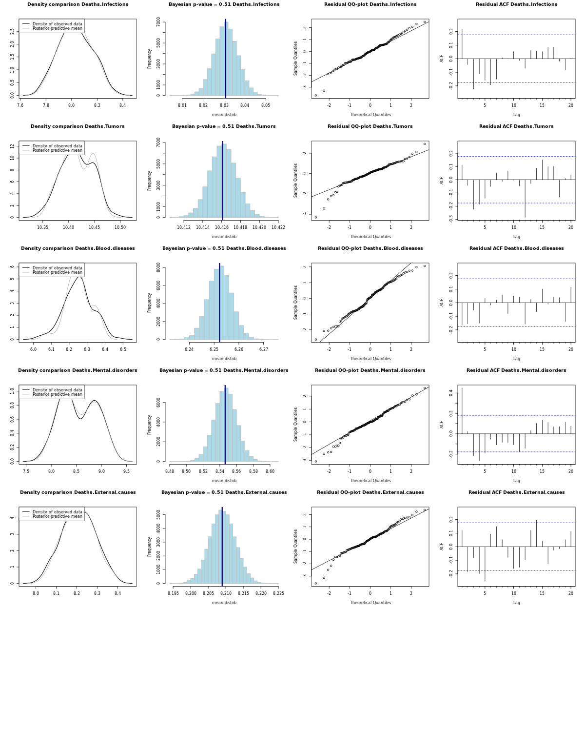
Figure S.25: Posterior predictive checks of control outcomes under Model 2.

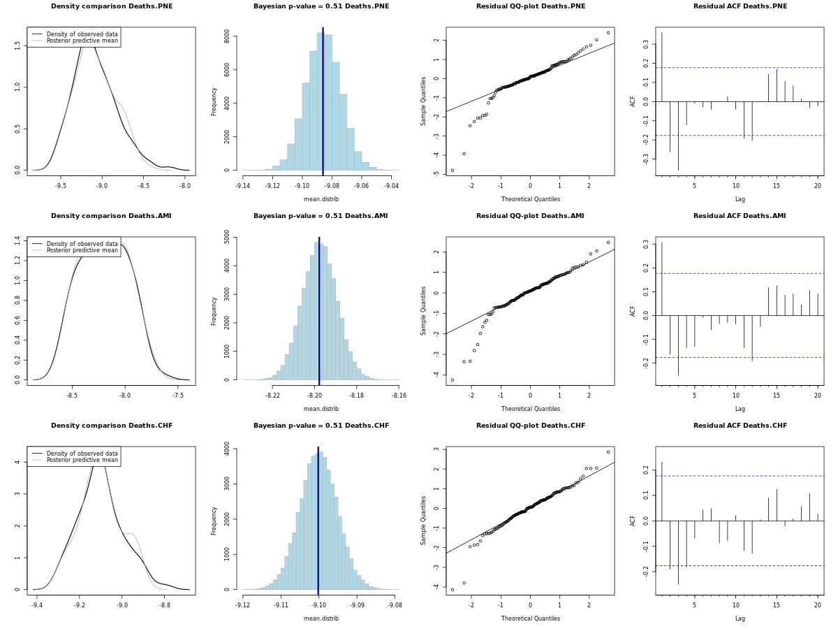
Figure S.26: Posterior predictive checks for pneumonia, AMI and CHF under Model 3.

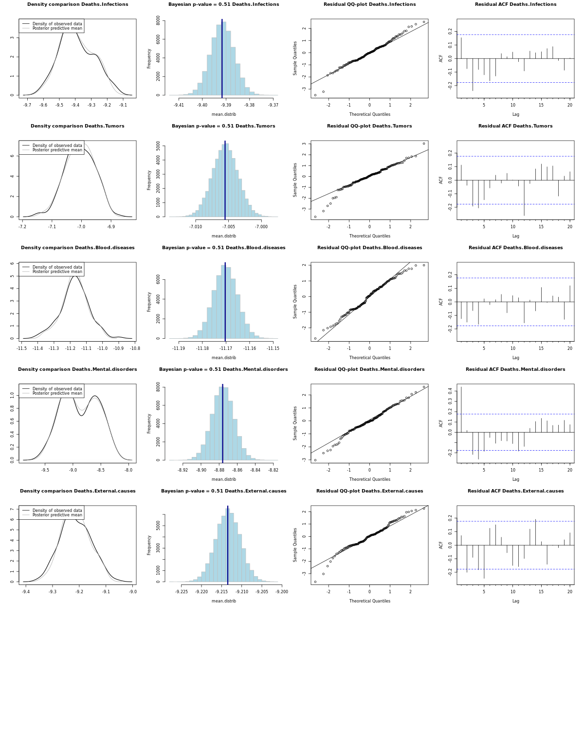
Figure S.27: Posterior predictive checks of control outcomes under Model 3.

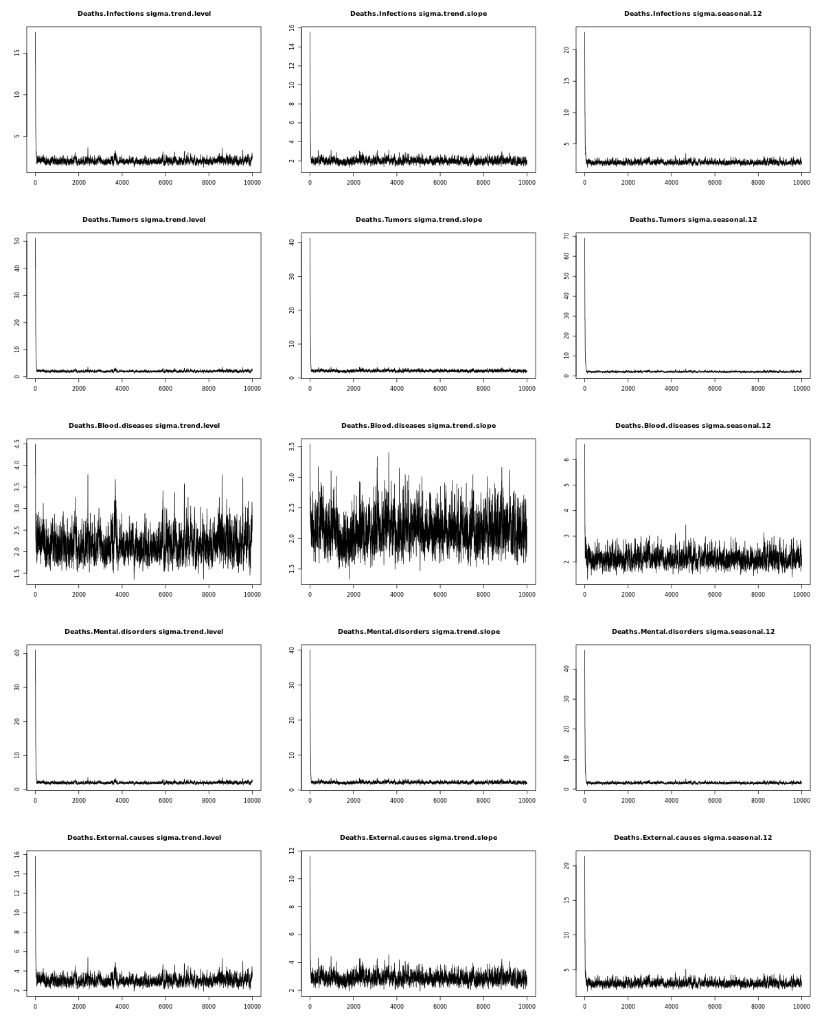
Figure S.28: Trace plots of control outcomes, Model 1.

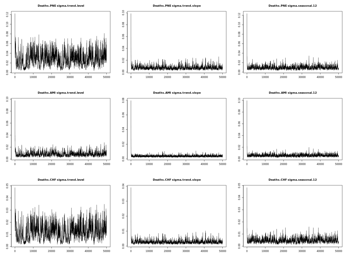
Figure S.29: Trace plots of pneumonia, AMI and CHF, Model 2.

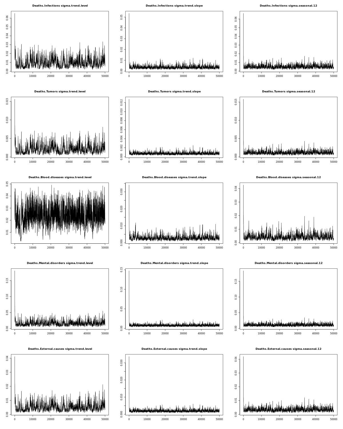
Figure S.30: Trace plots of control outcomes, Model 2.

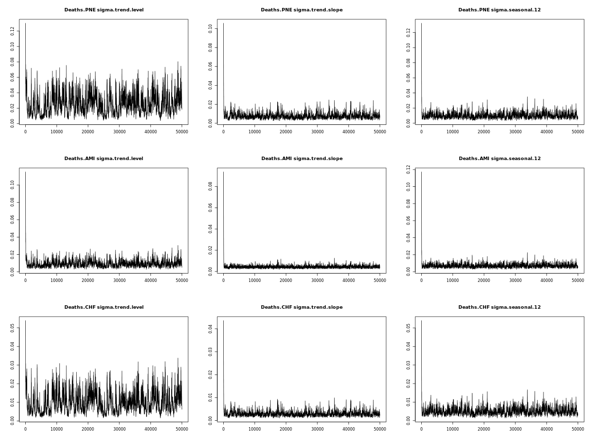
Figure S.31: Trace plots of pneumonia, AMI and CHF, Model 3.

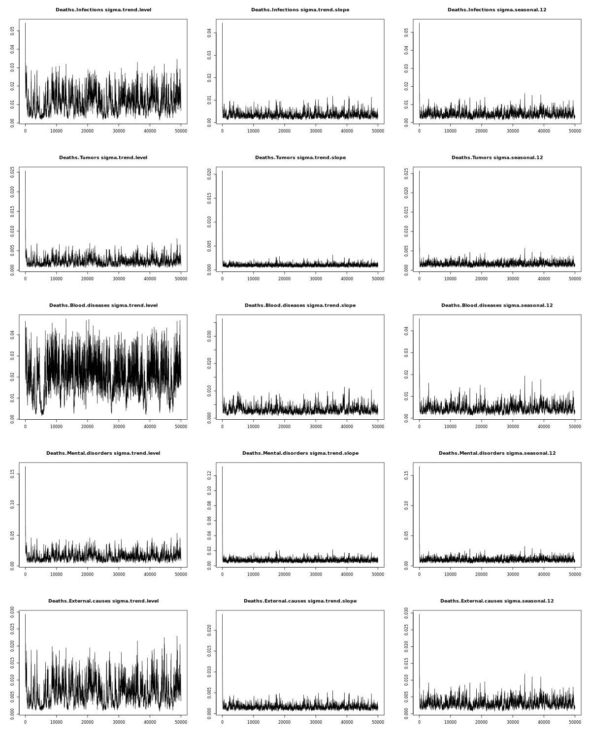
Figure S.32: Trace plots of control outcomes, Model 3.

The results from Model 1 are reported in the main paper: Table 2 shows the results for pneumonia, AMI and CHF, and Table 5 for the control outcomes. The results from Models 2 and 3 are shown, respectively, in Tables S.7 and S.8.

Table S.7: Falsification tests. Cumulative causal effect under Model 2 of the HRRP on pneumonia, AMI, CHF and control outcomes at three different time horizons.

Short term Mid term Long term C$\Delta$ 2.5% 97.5% C$\Delta$ 2.5% 97.5% C$\Delta$ 2.5% 97.5% Infections 3.34 -2.52 9.47 24.57 -55.67 109.83 61.96 -214.54 347.36 Tumors -0.02 -1.37 1.28 -0.04 -17.23 17.13 -0.75 -59.68 56.74 Blood diseases 2.08 -4.19 8.26 12.55 -61.85 86.91 30.27 -218.14 279.57 Mental disorders 2.55 -9.90 15.19 8.26 -161.50 180.53 -2.75 -586.00 583.10 External causes 1.56 -1.79 4.90 10.72 -33.35 55.35 28.37 -122.29 179.93 PNE 4.82 -8.19 18.30 31.00 -143.80 217.25 71.56 -524.20 689.68 AMI 1.58 -4.80 7.93 12.92 -71.28 97.64 35.55 -255.12 325.17 CHF 0.53 -4.85 5.65 5.80 -62.20 73.23 12.99 -220.14 239.62

Table S.8: Falsification tests. Cumulative causal effect under Model 3 of the HRRP on pneumonia, AMI, CHF and on control outcomes at three different time horizons.

Short term Mid term Long term C$\Delta$ 2.5% 97.5% C$\Delta$ 2.5% 97.5% C$\Delta$ 2.5% 97.5% Infections 22.60 -57.12 108.52 22.60 -57.12 108.52 56.28 -214.23 341.62 Tumors -1.06 -23.67 21.92 -1.06 -23.67 21.92 -4.29 -82.59 73.78 Blood diseases 11.63 -65.20 88.87 11.63 -65.20 88.87 27.14 -238.31 290.89 Mental disorders 6.89 -151.77 169.76 6.89 -151.77 169.76 -2.61 -551.91 549.90 External causes 8.74 -29.90 48.35 8.74 -29.90 48.35 22.41 -109.14 156.49 PNE 27.35 -148.24 212.29 27.35 -148.24 212.29 68.96 -534.68 694.65 AMI 11.22 -84.77 108.43 11.22 -84.77 108.43 32.57 -301.70 364.83 CHF 4.06 -65.13 73.23 4.06 -65.13 73.23 9.25 -227.97 242.20

At first sight, it might seem strange that Model 1 evidences some effect of the HRRP on pneumonia and AMI while Model 2 and 3 do not seem to spot any impact. However, this difference can be explained once we carefully consider the quantities that Models 1–3 estimate. Indeed, Model 1 targets an effect at the additive scale, while Models 2-3 target an effect at the multiplicative scale. More formally, let $Y_{t}$ be the death counts from a generic disease at time $t$ and let $y_{t}=\log{Y_{t}}$. In addition, denote with $R_{t}$ the mortality rate and let $r_{t}=\operatorname{logit}R_{t}$ denote its logit transformation, i.e.,

$$\operatorname{logit}R_{t}=\log{\frac{R_{t}}{1-R_{t}}}.$$

Then, under Model 1 the causal effect that we are estimating is:

$$\hat{\tau}_{t}^{(1)}=Y_{t}(1)-Y_{t}(0),$$

under Model 2 the effect is:

$$\hat{\tau}_{t}^{(2)}=y_{t}(1)-y_{t}(0)=\log{\frac{Y_{t}(1)}{Y_{t}(0)}},$$

and under Model 3 it is:

$$\hat{\tau}_{t}^{(3)}=r_{t}(1)-r_{t}(0)=\log{\frac{R_{t}(1)/(1-R_{t}(1))}{R_{t}(0)/(1-R_{t}(0))}}=\log{\Omega_{t}}$$

where $\Omega_{t}$ is the odds ratio (i.e., the ratio between the odds of dying and the odds of dying that over 65 people would have if HRRP was never adopted). Therefore, our results seem to show that there is no multiplicative effect of the treatment and there is no indication of an increase/decrease in the odds ratio, meaning that the odds of dying wouldn’t have been higher/lower in the absence of the HRRP. However, the data support the conclusion that there is a positive additive effect of the death counts.

References

- Abadie and Gardeazabal [2003] Alberto Abadie and Javier Gardeazabal. The economic costs of conflict: A case study of the Basque Country. American economic review, 93(1):113–132, 2003.
- Abadie et al. [2010] Alberto Abadie, Alexis Diamond, and Jens Hainmueller. Synthetic control methods for comparative case studies: Estimating the effect of California’s tobacco control program. Journal of the American Statistical Association, 105:493–505, 2010.
- Abadie et al. [2015] Alberto Abadie, Alexis Diamond, and Jens Hainmueller. Comparative politics and the synthetic control method. American Journal of Political Science, 59:495–510, 2015.
- Agresti [2013] Alan Agresti. Categorical data analysis. John Wiley & Sons, 2013.
- Angrist and Pischke [2008] Joshua D Angrist and Jörn-Steffen Pischke. Mostly harmless econometrics: An empiricist’s companion. Princeton University Press, Princeton, NJ, 2008.
- Antonelli and Beck [2020] Joseph Antonelli and Brenden Beck. Heterogeneous causal effects of neighborhood policing in new york city with staggered adoption of the policy. arXiv preprint arXiv:2006.07681, 2020.
- Athey and Imbens [2006] Susan Athey and Guido W. Imbens. Identification and Inference in Nonlinear Difference-in-Differences Models. Econometrica, 74(2):431–497, mar 2006. ISSN 0012-9682. doi: 10.1111/j.1468-0262.2006.00668.x. URL http://doi.wiley.com/10.1111/j.1468-0262.2006.00668.x.
- Ben-Michael et al. [2021] Eli Ben-Michael, Avi Feller, and Jesse Rothstein. The augmented synthetic control method. Journal of the American Statistical Association, 116(536):1789–1803, 2021.
- Bernal et al. [2017] James Lopez Bernal, Steven Cummins, and Antonio Gasparrini. Interrupted time series regression for the evaluation of public health interventions: a tutorial. International journal of epidemiology, 46(1):348–355, 2017.
- Bojinov and Shephard [2019] Iavor Bojinov and Neil Shephard. Time series experiments and causal estimands: exact randomization tests and trading. Journal of the American Statistical Association, 114(528):1665–1682, 2019.
- Brockwell and Davis [2009] Peter J Brockwell and Richard A Davis. Time series: theory and methods. Springer science & business media, 2009.
- Brodersen et al. [2015] Kay H Brodersen, Fabian Gallusser, Jim Koehler, Nicolas Remy, and Steven L Scott. Inferring causal impact using Bayesian structural time-series models. The Annals of Applied Statistics, 9(1):247–274, 2015. doi: 10.1214/14-AOAS788. URL https://static.googleusercontent.com/media/research.google.com/en//pubs/archive/41854.pdf.
- Card and Krueger [1993] David Card and Alan B Krueger. Minimum wages and employment: A case study of the fast food industry in New Jersey and Pennsylvania. Technical report, Working Paper No. 4509, National Bureau of Economic Research, 1993.
- Casalino et al. [2007] Lawrence P Casalino, Arthur Elster, Andy Eisenberg, Evelyn Lewis, John Montgomery, and Diana Ramos. Will pay-for-performance and quality reporting affect health care disparities? these rapidly proliferating programs do not appear to be devoting much attention to the possible impact on disparities in health care. Health affairs, 26(Suppl2):w405–w414, 2007.
- Coxe et al. [2009] Stefany Coxe, Stephen G West, and Leona S Aiken. The analysis of count data: A gentle introduction to poisson regression and its alternatives. Journal of personality assessment, 91(2):121–136, 2009.
- Cruz et al. [2017] Maricela Cruz, Miriam Bender, and Hernando Ombao. A robust interrupted time series model for analyzing complex health care intervention data. Statistics in medicine, 36(29):4660–4676, 2017.
- Desai et al. [2016] Nihar R Desai, Joseph S Ross, Ji Young Kwon, Jeph Herrin, Kumar Dharmarajan, Susannah M Bernheim, Harlan M Krumholz, and Leora I Horwitz. Association Between Hospital Penalty Status Under the Hospital Readmission Reduction Program and Readmission Rates for Target and Nontarget Conditions. Journal of the American Medical Association, 316(24):2647–2656, 2016. ISSN 1538-3598. doi: 10.1001/jama.2016.18533. URL http://www.ncbi.nlm.nih.gov/pubmed/28027367http://www.pubmedcentral.nih.gov/articlerender.fcgi?artid=PMC5599851.
- Dharmarajan et al. [2017] Kumar Dharmarajan, Yongfei Wang, Zhenqiu Lin, Sharon Lise T. Normand, Joseph S. Ross, Leora I. Horwitz, Nihar R. Desai, Lisa G. Suter, Elizabeth E. Drye, Susannah M. Bernheim, and Harlan M. Krumholz. Association of changing hospital readmission rates with mortality rates after hospital discharge. JAMA - Journal of the American Medical Association, 318(3):270–278, 2017. ISSN 15383598. doi: 10.1001/jama.2017.8444.
- Doudchenko and Imbens [2016] N Doudchenko and GW Imbens. Balancing, regression, difference-in-differences and synthetic control methods: A synthesis. no. 22791. National Bureau of Economic Research, 2016.
- Doudchenko and Imbens [2017] Nikolay Doudchenko and Guido W Imbens. Balancing, Regression, Difference-In-Differences and Synthetic Control Methods: A Synthesis. arXiv preprint arXiv:1610.07748v2, 2017.
- Fonarow et al. [2017] Gregg C. Fonarow, Marvin A. Konstam, and Clyde W. Yancy. The Hospital Readmission Reduction Program Is Associated With Fewer Readmissions, More Deaths: Time to Reconsider. Journal of the American College of Cardiology, 70(15):1931–1934, 2017. ISSN 15583597. doi: 10.1016/j.jacc.2017.08.046.
- Gaughan et al. [2019] James Gaughan, Nils Gutacker, Katja Grašič, Noemi Kreif, Luigi Siciliani, and Andrew Street. Paying for efficiency: Incentivising same-day discharges in the english nhs. Journal of health economics, 68:102226, 2019.
- Gelman et al. [1996] Andrew Gelman, Xiao-Li Meng, and Hal Stern. Posterior predictive assessment of model fitness via realized discrepancies. Statistica sinica, 1996.
- Gelman et al. [2013] Andrew Gelman, John B Carlin, Hal S Stern, David B Dunson, Aki Vehtari, and Donald B Rubin. Bayesian data analysis. CRC press, 2013.
- Griffin et al. [2022] Beth Ann Griffin, Megan S Schuler, Joseph Pane, Stephen W Patrick, Rosanna Smart, Bradley D Stein, Geoffrey Grimm, and Elizabeth A Stuart. Methodological considerations for estimating policy effects in the context of co-occurring policies. Health Services and Outcomes Research Methodology, pages 1–17, 2022.
- Gupta et al. [2017] Ankur Gupta, Larry A. Allen, Deepak L. Bhatt, Margueritte Cox, Adam D. DeVore, Paul A. Heidenreich, Adrian F. Hernandez, Eric D. Peterson, Roland A. Matsouaka, Clyde W. Yancy, and Gregg C. Fonarow. Association of the hospital readmissions reduction program implementation with readmission and mortality outcomesin heart failure. JAMA Cardiology, 3(1):44–53, 2017. ISSN 23806591. doi: 10.1001/jamacardio.2017.4265.
- Huckfeldt et al. [2019] Peter Huckfeldt, José Escarce, Neeraj Sood, Zhiyou Yang, Ioana Popescu, and Teryl Nuckols. Thirty-Day Postdischarge Mortality Among Black and White Patients 65 Years and Older in the Medicare Hospital Readmissions Reduction ProgramPostdischarge Mortality Among Black and White Patients With MedicarePostdischarge Mortality Among Black and White P. JAMA Network Open, 2(3):e190634–e190634, mar 2019. ISSN 2574-3805. doi: 10.1001/jamanetworkopen.2019.0634. URL https://doi.org/10.1001/jamanetworkopen.2019.0634.
- Imbens and Rubin [2015] Guido W Imbens and Donald B Rubin. Causal inference in Statistics, Social, and Biomedical Sciences. Cambridge University Press, Cambridge, UK, 2015.
- Joynt and Jha [2012] Karen E. Joynt and Ashish K. Jha. Thirty-Day Readmissions — Truth and Consequences. New England Journal of Medicine, 366(15):1366–1369, apr 2012. ISSN 0028-4793. doi: 10.1056/NEJMp1201598. URL http://www.nejm.org/doi/abs/10.1056/NEJMp1201598.
- Joynt et al. [2011] Karen E. Joynt, E. John Orav, and Ashish K. Jha. Thirty-Day Readmission Rates for Medicare Beneficiaries by Race and Site of Care. Journal of the American Medical Association, 305(7):675, feb 2011. doi: 10.1001/jama.2011.123. URL http://jama.jamanetwork.com/article.aspx?doi=10.1001/jama.2011.123.
- Khera et al. [2018] Rohan Khera, Kumar Dharmarajan, Yongfei Wang, Zhenqiu Lin, Susannah M Bernheim, Yun Wang, Sharon-Lise T Normand, and Harlan M Krumholz. Association of the Hospital Readmissions Reduction Program With Mortality During and After Hospitalization for Acute Myocardial Infarction, Heart Failure, and PneumoniaAssociation of Hospital Readmissions Reduction Program With MortalityAssociation of Hos. JAMA Network Open, 1(5):e182777–e182777, sep 2018. ISSN 2574-3805. doi: 10.1001/jamanetworkopen.2018.2777. URL https://doi.org/10.1001/jamanetworkopen.2018.2777.
- McDowall et al. [2019] David McDowall, Richard McCleary, and Bradley J Bartos. Interrupted time series analysis. Oxford University Press, 2019.
- Medina-Ramón et al. [2006] Mercedes Medina-Ramón, Antonella Zanobetti, David Paul Cavanagh, and Joel Schwartz. Extreme temperatures and mortality: assessing effect modification by personal characteristics and specific cause of death in a multi-city case-only analysis. Environmental health perspectives, 114(9):1331–1336, 2006.
- MedPAC [2018] MedPAC. The effects of the Hospital Readmissions Reduction Program. Technical report, 2018. URL http://www.medpac.gov/docs/default-source/reports/jun18{_}ch1{_}medpacreport{_}sec.pdf?sfvrsn=0.
- Menchetti et al. [2021] Fiammetta Menchetti, Fabrizio Cipollini, and Fabrizia Mealli. Combining counterfactual outcomes and ARIMA models for policy evaluation. Forthcoming. The Econometrics Journal. Earlier version available at https://arxiv.org/abs/2103.06740, 2021.
- Meyer et al. [1995] Bruce D Meyer, W Kip Viscusi, and David L Durbin. Workers’ compensation and injury duration: Evidence from a natural experiment. American economic review, 85(3):322–340, 1995.
- Miratrix [2020] Luke Miratrix. Package simits: Analysis via simulation of interrupted time series (ITS) data. 2020.
- Miratrix et al. [2019] Luke Miratrix, Chloe Anderson, Brittany Henderson, Cindy Redcross, and Erin Valentine. Simulating for uncertainty with interrupted time series designs. Technical report, 2019. URL https://www.mdrc.org/sites/default/files/img/methods{_}for{_}ITS.pdf.
- O’Neill et al. [2016] Stephen O’Neill, Noémi Kreif, Richard Grieve, Matthew Sutton, and Jasjeet S Sekhon. Estimating causal effects: Considering three alternatives to difference-in-differences estimation. Health Services and Outcomes Research Methodology, 16:1–21, 2016.
- Ryan et al. [2015] Andrew M Ryan, James F Burgess Jr, and Justin B Dimick. Why we should not be indifferent to specification choices for difference-in-differences. Health services research, 50:1211–1235, 2015.
- Sandhu and Heidenreich [2019] Alexander T. Sandhu and Paul A. Heidenreich. Comparison of the change in heart failure readmission and mortality rates between hospitals subject to hospital readmission reduction program penalties and critical access hospitals. American Heart Journal, 209:63–67, 2019. ISSN 10976744. doi: 10.1016/j.ahj.2018.12.002. URL https://doi.org/10.1016/j.ahj.2018.12.002.
- Schaffer et al. [2021] Andrea L Schaffer, Timothy A Dobbins, and Sallie-Anne Pearson. Interrupted time series analysis using autoregressive integrated moving average (ARIMA) models: a guide for evaluating large-scale health interventions. BMC medical research methodology, 21(1):1–12, 2021.
- Wadhera et al. [2018] Rishi K. Wadhera, Karen E. Joynt Maddox, Jason H. Wasfy, Sebastien Haneuse, Changyu Shen, and Robert W. Yeh. Association of the Hospital Readmissions Reduction Program with Mortality among Medicare Beneficiaries Hospitalized for Heart Failure, Acute Myocardial Infarction, and Pneumonia. JAMA - Journal of the American Medical Association, 320(24):2542–2552, 2018. ISSN 15383598. doi: 10.1001/jama.2018.19232.
- Wadhera et al. [2019] Rishi K Wadhera, Karen E Joynt Maddox, Dhruv S Kazi, Changyu Shen, and Robert W Yeh. Hospital revisits within 30 days after discharge for medical conditions targeted by the Hospital Readmissions Reduction Program in the United States: national retrospective analysis. BMJ, 366(l4563), 2019. doi: 10.1136/bmj.l4563. URL http://dx.doi.org/10.1136/bmj.l4563.
- Wagner et al. [2002] Anita K Wagner, Stephen B Soumerai, Fang Zhang, and Dennis Ross-Degnan. Segmented regression analysis of interrupted time series studies in medication use research. Journal of clinical pharmacy and therapeutics, 27(4):299–309, 2002.
- Wasfy et al. [2017] Jason H Wasfy, Corwin Matthew Zigler, Christine Choirat, Yun Wang, Francesca Dominici, and Robert W Yeh. Readmission Rates After Passage of the Hospital Readmissions Reduction Program: A Pre–Post Analysis. Annals of Internal Medicine, 166(5):324–331, 2017. doi: 10.7326/M16-0185. URL https://www.ncbi.nlm.nih.gov/pmc/articles/PMC5507076/pdf/nihms869067.pdf.
- West and Harrison [2006] Mike West and Jeff Harrison. Bayesian forecasting and dynamic models. Springer-Verlag, New York, NY, 2006.
- Wheeler [2018] Andrew P Wheeler. The effect of 311 calls for service on crime in dc at microplaces. Crime & delinquency, 64(14):1882–1903, 2018.
- Ye et al. [2022] Shangyuan Ye, Rui Wang, and Bo Zhang. Comparison of estimation methods and sample size calculation for parameter-driven interrupted time series models with count outcomes. Health Services and Outcomes Research Methodology, pages 1–48, 2022.
- Zigler and Papadogeorgou [2021] Corwin M Zigler and Georgia Papadogeorgou. Bipartite causal inference with interference. Statistical science: a review journal of the Institute of Mathematical Statistics, 36(1):109, 2021.
- Zuckerman et al. [2016] Rachael B. Zuckerman, Steven H. Sheingold, E. John Orav, Joel Ruhter, and Arnold M. Epstein. Readmissions, Observation, and the Hospital Readmissions Reduction Program. New England Journal of Medicine, 374(16):1543–1551, apr 2016. ISSN 0028-4793. doi: 10.1056/NEJMsa1513024. URL http://www.nejm.org/doi/10.1056/NEJMsa1513024.