Crossover from anomalous to normal diffusion: truncated power-law noise correlations and applications to dynamics in lipid bilayers

Abstract

The emerging diffusive dynamics in many complex systems shows a characteristic crossover behaviour from anomalous to normal diffusion which is otherwise fitted by two independent power-laws. A prominent example for a subdiffusive-diffusive crossover are viscoelastic systems such as lipid bilayer membranes, while superdiffusive-diffusive crossovers occur in systems of actively moving biological cells. We here consider the general dynamics of a stochastic particle driven by so-called tempered fractional Gaussian noise, that is noise with Gaussian amplitude and power-law correlations, which are cut off at some mesoscopic time scale. Concretely we consider such noise with built-in exponential or power-law tempering, driving an overdamped Langevin equation (fractional Brownian motion) and fractional Langevin equation motion. We derive explicit expressions for the mean squared displacement and correlation functions, including different shapes of the crossover behaviour depending on the concrete tempering, and discuss the physical meaning of the tempering. In the case of power-law tempering we also find a crossover behaviour from faster to slower superdiffusion and slower to faster subdiffusion. As a direct application of our model we demonstrate that the obtained dynamics quantitatively described the subdiffusion-diffusion and subdiffusion-subdiffusion crossover in lipid bilayer systems. We also show that a model of tempered fractional Brownian motion recently proposed by Sabzikar and Meerschaert leads to physically very different behaviour with a seemingly paradoxical ballistic long time scaling.

1 Introduction

Diffusion, the stochastic motion of a tracer particle, was beautifully described by Brown in his study of pollen granules and a multitude of other molecules (microscopic particles) [1]. Diffusion is typically described in terms of the mean squared displacement (MSD)

$$\langle x^{2}(t)\rangle\simeq\mathcal{D}_{\alpha}t^{\alpha}$$ (1)

of the particle spreading. When $\alpha=1$ this is the well known law of normal (Brownian or Fickian) diffusion observed in detailed quantitative studies by Perrin, Nordlund, and Kappler [2, 3, 4], among others. In the case of a scaling with an exponent $\alpha$ different from unity, the dynamics encoded by the MSD (1) can be classified in terms of the anomalous diffusion exponent $\alpha$ as either subdiffusive for $0<\alpha<1$ or superdiffusive for $\alpha>1$ [5, 6]. In expression (1) the generalised diffusion coefficient has physical dimension $[\mathcal{D}_{\alpha}]=\mathrm{cm}^{2}/\mathrm{s}^{\alpha}$. Anomalous diffusion with $\alpha\neq 1$ has been revealed in a multitude of systems [5, 6, 7]. In particular, following the massive advances of microscopy techniques anomalous diffusion was discovered in a surging number of biological systems [8, 9]. Thus, subdiffusion was monitored for both endogenous and introduced submicron tracers in biological cells [10, 11, 12, 13, 14, 15, 16, 17] or in inanimate, artificially crowded systems [18, 19, 20]. Supercomputing studies of protein internal motion [21] or of constituent molecules of dilute and protein-crowded lipid bilayer membranes [22, 23, 24, 25, 26] also show subdiffusive behaviour. Due to active motion, also superdiffusion has been reported from several cellular systems [10, 11, 27, 28, 29]. For a more exhaustive list of systems see the recent reviews [8, 9, 30, 31, 32].

In most of these systems the observed anomalous diffusion was identified as fractional Brownian motion or fractional Langevin equation motion type defined below. Both are characterised by power-law correlations of the driving noise [7, 8, 33]. At sufficiently long times, however, this anomalous diffusion will eventually cross over to normal diffusion, when the system’s temporal evolution exceeds some relevant correlation time. For instance, all atom molecular dynamics simulations of pure lipid bilayer membranes exhibit a subdiffusive-diffusive crossover at around 10 nsec, the time scale when two lipids mutually exchange their position [22]. The quantitative description of this anomalous-to-normal crossover is the topic of this paper. For both the subdiffusive and superdiffusive situations we include a maximum correlation time of the driving noise and provide exact solutions for the MSD in the case of hard, exponential and power-law truncation, so-called tempering, that can be easily applied in the analysis of experimental or simulations data. The advantage of such a model, in comparison to simply combining an anomalous and a normal diffusive law for the MSD is that the crossover is built into a two-parameter exponential tempering model depending only on the noise strength driving the motion and the crossover time. For the case of a power-law tempering an additional scaling exponent enters. Depending on its magnitude, the anomalous-normal crossover dynamics can be extended to a crossover from either faster to slower superdiffusion or slower to faster subdiffusion. In this approach the crossover between different diffusion regimes thus naturally emerges, and the type of tempering governs the exact crossover shape. As we will show the crossover shape encoded in this approach nicely fits actual data.

The paper is structured as follows. In section 2 we consider the tempering of superdiffusive fractional Brownian motion and derive the crossover to normal diffusion. In section 3 we perform the same tasks for the subdiffusive generalised Langevin equation. Section 3.5 compares our subdiffusive to normal diffusive model of the tempered generalised Langevin equation to supercomputing data from lipid bilayer membranes exhibiting characteristic crossover dynamics. The data analysis demonstrates excellent agreement with the built-in crossover behaviour of our model. Section 4 addresses direct tempering suggested by Meerschaert and Sabzikar as well as its physicality. Indeed, we show that this type of tempering leads to ballistic motion. We conclude in section 5. Several short appendices provide some additional mathematical details.

2 Tempered superdiffusive fractional Brownian motion

We start from the overdamped stochastic equation of motion of a physical test particle in a viscous medium under the influence of a stochastic force $\xi(t)$ [34, 35]

$$\frac{dx(t)}{dt}=\frac{\xi(t)}{m\eta}=v(t),$$ (2)

where $x(t)$ is the particle position and $v(t)$ its velocity. Without loss of generality we assume the initial condition $x(0)=0$. Furthermore, $m$ is the particle mass, and $\eta$, of physical dimension $[\eta]=\mathrm{s}^{-1}$ is the friction coefficient. The stochastic force $\xi(t)$ is assumed to be a stationary and Gaussian noise of zero mean. Then the velocity autocorrelation function fulfils

$$\langle v(t)v(t+\tau)\rangle=\langle v^{2}\rangle_{\tau},$$ (3)

for all $\tau\geq 0$. By formal integration of equation (2) the MSD yields in the form

$$\langle x^{2}(t)\rangle = \int_{0}^{t}dt_{1}\int_{0}^{t}dt_{2}\langle v(t_{1})v(t_{2})\rangle$$ (4)

$$= 2\int_{0}^{t}dt_{1}\int_{t_{1}}^{t}dt_{2}\langle v(t_{1})v(t_{2})\rangle=2\int_{0}^{t}d\tau(t-\tau)\langle v^{2}\rangle_{\tau}.$$

From this result we infer that if the autocorrelation function $\langle v^{2}\rangle_{\tau}$ decays sufficiently fast at long times, such that $\int_{0}^{\infty}d\tau\langle v^{2}\rangle_{\tau}$ is finite, then the MSD reads

$$\langle x^{2}(t)\rangle\sim 2t\int_{0}^{\infty}d\tau\langle v^{2}\rangle_{\tau},$$ (5)

at $t\to\infty$, and diffusion becomes asymptotically normal. Thus, one should expect anomalous diffusion at long times whenever $\int_{0}^{\infty}d\tau\langle v^{2}\rangle_{\tau}$ is either infinity or zero. This is exactly the case for the persistent and antipersistent fractional Gaussian motions considered in what follows, respectively. In the case of superdiffusive fractional Brownian motion we choose the autocorrelation function in the form

$$\langle v^{2}\rangle_{\tau}=\frac{\mathcal{D}_{H}}{\Gamma(2H-1)}\tau^{2H-2},$$ (6)

where the constant noise strength $\mathcal{D}_{H}$ has dimension $[\mathcal{D}_{H}]=\mathrm{cm}^{2}/\mathrm{s}^{2H}$, $\Gamma(z)$ is the Gamma function, and the Hurst exponent $H$ is in the interval $1/2\leq H<1$. We note here that this approach leads to the correct power-law asymptotics of the classical Mandelbrot-van Ness fractional Gaussian noise at long times [36] with $\int_{0}^{\infty}d\tau\langle v^{2}\rangle_{\tau}=\infty$, but at the same time leads to an infinite zero-point variance $\langle v^{2}\rangle_{\tau=0}$ of the noise. Keeping away from $\tau=0$ we are allowed to restrict ourselves to the power-law form (6). Furthermore the coefficient $\Gamma(2H-1)$ in equation (6) is introduced to capture the white noise limit. Indeed, due to the property of the $\delta$-function [37]

$$\lim_{H\to 0.5^{+}}\frac{\tau^{2H-2}}{\Gamma(2H-1)}=\delta(\tau)$$ (7)

at $H=0.5$ and with $\int_{0}^{\infty}d\tau\delta(\tau)=1$ equation (6) reduces to

$$\langle v^{2}\rangle_{\tau}=\mathcal{D}\delta(\tau)$$ (8)

with $\mathcal{D}_{1/2}=\mathcal{D}$.

Now, after plugging result (6) into expression (4) the MSD can be readily calculated, yielding

$$\langle x^{2}(t)\rangle=\frac{2\mathcal{D}_{H}}{\Gamma(2H+1)}t^{2H},$$ (9)

which yields sub-ballistic superdiffusion with the anomalous diffusion exponent $\alpha=2H$, and thus $1<\alpha<2$.

In what follows we consider both a hard exponential and a power-law truncation (tempering) of the persistent fractional Gaussian noise with Hurst exponent $1/2\leq H<1$.

2.1 Exponentially truncated fractional Gaussian noise

Let us first consider an exponential tempering of the form

$$\langle v^{2}\rangle_{\tau}=\frac{\mathcal{D}_{H}}{\Gamma(2H-1)}\tau^{2H-2}e^{-\tau/\tau_{\star}},$$ (10)

for $\tau>0$, where $\tau_{\star}>0$ is a characteristic crossover time scale. For instance, in the case of moving cells the crossover time $\tau_{\star}$ would correspond to the time scale when the cell motion becomes uncorrelated, similar to the decorrelation of the lipid motion in the example of the lipid bilayer system discussed below.

Here we note that one should keep in mind that the autocorrelation function $\langle v^{2}\rangle_{\tau}$ can not be chosen arbitrary. Namely, its Fourier transform, the spectrum $\langle\tilde{v}^{2}(\omega)\rangle$ of the random process $v(t)$ must be non-negative [41]. The positivity of $\langle\tilde{v}^{2}(\omega)\rangle$ for the case of exponential tempering in equation (10) is shown in A. Note also that now $\int_{0}^{\infty}d\tau\langle v^{2}\rangle_{\tau}=\mathcal{D}_{H}\tau_{\star}^{2H-1}$ is finite, thus we expect normal diffusion at long times.

With the use of expression (4) the MSD for the exponentially truncated fractional Gaussian noise takes on the exact form

$$\langle x^{2}(t)\rangle=\frac{2\mathcal{D}_{H}\tau_{\star}^{2H}}{\Gamma(2H-1)}\left[\frac{t}{\tau_{\star}}\gamma\left(2H-1,\frac{t}{\tau_{\star}}\right)-\gamma\left(2H,\frac{t}{\tau_{\star}}\right)\right],$$ (11)

where $\gamma(a,z)=\int_{0}^{z}t^{a-1}e^{-t}dt$ is the incomplete $\gamma$-function. Using the asymptotic $\gamma(a,z)\sim z^{a}/a$ for $z\ll 1$, and $\gamma(a,z)\sim\Gamma(a)$ for $z\gg 1$, we observe superdiffusive behaviour at short times, and normal diffusion at long times, namely,

$$\langle x^{2}(t)\rangle\sim\left\{\begin{array}[]{ll}\frac{\displaystyle 2\mathcal{D}_{H}}{\displaystyle\Gamma(2H+1)}t^{2H},&t\ll\tau_{\star}\\[17.07182pt] 2\mathcal{D}_{H}\tau_{\star}^{2H-1}t,&t\gg\tau_{\star}.\end{array}\right.$$ (12)

The emerging normal diffusion thus has the effective diffusivity $\mathcal{D}_{H}\tau_{\star}^{2H-1}$. Note that the approximate formula at long times is in concordance with the simple estimate given by expression (5).

Figure 1 shows the crossover behaviour from superdiffusion to normal diffusion encoded in expression (11), along with the short and long time asymptotes given by result (12). As can be discerned from the plot, the crossover region is fairly short, spanning less than a decade in time for the chosen parameters.

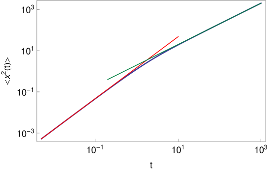
Figure 1: Mean squared displacement (11) for superdiffusive fractional Brownian motion with $H=3/4$, $\mathcal{D}_{H}=1$, and $\tau_{\star}=1$ (blue line). The short and long time asymptotics given by expression (12) are depicted by the red and green lines, respectively.

2.2 Power-law truncated fractional Gaussian noise

We now consider the softer power-law truncation of the form

$$\langle v^{2}\rangle_{\tau}=\frac{\mathcal{D}_{H}}{\Gamma(2H-1)}\tau^{2H-2}\left(1+\frac{\tau}{\tau_{\star}}\right)^{-\mu},$$ (13)

for $\tau>0$, $\mu>0$ and compare the resulting behaviour with the scenario of exponential tempering. Here, apart from the crossover time $\tau_{\star}$ the new power-law exponent $\mu$ is introduced which effects the dynamics at long times, as we are going to show below. We remark that the positivity of the spectrum for the power-law truncated form is discussed in A. After plugging (13) into expression (4) we find for the MSD that

$$\langle x^{2}(t)\rangle=\frac{2\mathcal{D}_{H}\tau_{\star}^{2H}}{\Gamma(2H-1)}\left[\frac{t}{\tau_{\star}}f\left(\mu,2H-1;\frac{t}{\tau_{\star}}\right)-f\left(\mu,2H;\frac{t}{\tau_{\star}}\right)\right],$$ (14)

where we introduced the notation

$$f(\mu,\alpha;a)=\int_{0}^{a}\frac{y^{\alpha-1}}{(1+y)^{\mu}}dy.$$ (15)

Now, using the integral representation [42] of the hypergeometric function ${}_{2}F_{1}$ [43] we rewrite the integral in equation (15) as

$$f(\mu,\alpha;a)=\frac{a^{\alpha}}{\alpha}{{}_{2}}F_{1}(\mu,\alpha,\alpha+1;-a),$$ (16)

and thus rewrite the MSD (14) in the final form

$$\langle x^{2}(t)\rangle = \frac{2\mathcal{D}_{H}t^{2H}}{\Gamma(2H-1)}\left[\frac{1}{2H-1}{{}_{2}}F_{1}\left(\mu,2H-1;2H;-\frac{t}{\tau_{\star}}\right)\right.$$ (17)

$$\hskip 62.59596pt\left.-\frac{1}{2H}{{}_{2}}F_{1}\left(\mu,2H;2H+1;-\frac{t}{\tau_{\star}}\right)\right],$$

In this notation the MSD can be directly evaluated by Wolfram Mathematica [44]. Note that ${}_{2}F_{1}(0,b;c;z)=1$, and thus result (17) reduces exactly to the MSD (9) for the untruncated case $\mu=0$. To obtain the limiting behaviours of the MSD (17) at short times $t\ll\tau_{\star}$ we use the Gauss hypergeometric series for the function ${}_{2}F_{1}$, see 15.1.1 in [42]. As result, to leading order we recover the MSD (9) of untruncated fractional Brownian motion.

At long times $t\gg\tau_{\star}$ the situation for power-law tempering is actually richer than for the case of exponential tempering. To see this, we first employ the linear transformation formula 15.3.7 in [42] and write expression (17) in the form

$$\langle x^{2}(t)\rangle = \frac{2D_{H}\tau_{\star}^{2H-1}t}{\Gamma(2H-1)}\left[\frac{\Gamma(2H-1)\Gamma(\mu+1-2H)}{\Gamma(\mu)}-\frac{\Gamma(2H+1)\Gamma(\mu-2H)}{2H\Gamma(\mu)}\frac{\tau_{\star}}{t}\right.$$ (18)

$$+\frac{1}{2H-\mu-1}\left(\frac{\tau_{\star}}{t}\right)^{\mu+1-2H}\,_{2}F_{1}\left(\mu,\mu+1-2H;\mu+2-2H;-\frac{\tau_{\star}}{t}\right)$$

$$\left.-\frac{1}{2H-\mu}\left(\frac{\tau_{\star}}{t}\right)^{\mu+1-2H}\,_{2}F_{1}\left(\mu,\mu-2H;\mu+1-2H;-\frac{\tau_{\star}}{t}\right)\right].$$

We consider two possible cases:

2.2.1 Weak power-law truncation, $0<\mu<2H-1<1$.

In this case the third and fourth terms in the square brackets of expression (18) are dominating and we find

$$\langle x^{2}(t)\rangle\sim\frac{2D_{H}\tau_{\star}^{\mu}}{(2H-\mu)(2H-1-\mu)\Gamma(2H-1)}t^{2H-\mu}$$ (19)

for $t\gg\tau_{\star}$. Note that in the limit $\mu\to 0$ result (19) reduces to the untruncated formula (9). Thus, since we observe the inequality $2H-\mu>1$ in the case of weak power-law truncation the dynamics is still superdiffusive, however, with a reduced anomalous diffusion exponent smaller than the value $2H$ in the short time limit.

2.2.2 Strong power-law truncation, $\mu>2H-1>0$.

Note that in this case the integral of the velocity autocorrelation function (13) over the whole time domain converges, $\int_{0}^{\infty}d\tau\langle v^{2}\rangle_{\tau}=\mathcal{D}_{H}\tau_{\star}^{2H-1}\Gamma(\mu-2H+1)/\Gamma(\mu)$, see 2.2.5.24 in [62]. Thus, with expression (5) we expect a linear time behaviour in the long time limit, whereas the term to next order in (4) gives $\int^{t}d\tau\tau\langle v^{2}\rangle_{\tau}\simeq\int^{t}d\tau\tau^{2H-1-\mu}\simeq t^{2H-\mu}$, a sublinear contribution since $2H-\mu<1$. Alternatively, it follows from (18) that the main contribution comes from the first term in the square brackets. Thus, in full accordance with expression (5) we get

$$\langle x^{2}(t)\rangle\sim\frac{\displaystyle 2\mathcal{D}_{H}\Gamma(\mu-2H+1)\tau_{\star}^{2H-1}t}{\displaystyle\Gamma(\mu)}$$ (20)

at $t\gg\tau_{\star}$.

Finally, for the borderline case $0<\mu=2H-1<1$ it is in fact easier to consider equation (17). Making use of formula 7.3.1.81 in [63] we see that the leading contribution comes from the first hypergeometric function in the square brackets in expression (17), as ${}_{2}F_{1}(2H-1,2H-1;2H;z)\sim\Gamma(2H)\Gamma^{-1}(2H-1)(-z)^{-2H+1}\ln(-z)$. For the MSD we then finally obtain

$$\langle x^{2}(t)\rangle\sim\frac{2D_{H}\tau_{\star}^{2H-1}}{\Gamma(2H-1)}t\ln\left(\frac{t}{\tau_{\star}}\right).$$ (21)

Thus, in this borderline limit between weak truncation (leading to reduced superdiffusion at long times) and strong truncation (normal long time diffusion) we here obtain normal diffusion with a logarithmic correction.

Figure 2 demonstrates that for the power-law tempering the crossover region is significantly enhanced, spanning several orders of magnitude, as compared to the much swifter crossover in the case of exponential tempering.

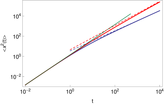
Figure 2: MSD (17) for power-law tempered fractional Brownian motion with $H=3/4$, $\mathcal{D}_{H}=1$, and $\tau_{\star}=1$. The red solid line is for $\mu=0.3$ (weak power law truncation), whereas the blue solid line is for $\mu=1$ (strong power-law truncation). The red and blue dashed lines correspond to the asymptotics (19) and (20), respectively. The behaviour for the untruncated case given by expression (9) is depicted by the green solid line.

The MSDs for both cases of exponential and power-law truncation are directly compared in figure 3, along with the time derivative of the MSD. As can be seen, the crossover for the exponential tempering occurs much more rapidly. Thus also the amplitude of the long time Brownian scaling is higher in the case of the power-law tempering for the same value of the crossover time scale $\tau_{\star}$.

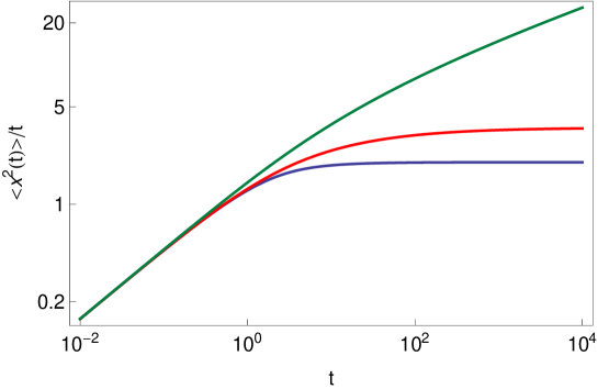
Figure 3: Comparison of the ratio $\langle x^{2}\rangle/t$ for different modes of truncation of the power-law noise in equation (2). Parameters: $H=3/4$, $D_{H}=1$, and $\tau_{\star}=1$. From bottom to top the blue line depicts the exponential truncation (11) while the red line and green lines show expression (17) for strong ($\mu=1$) and weak ($\mu=0.3$) power-law truncation, respectively.

A graphical representation of the correlation functions (6), (10) and (13) is given in figure 4. The exponential cutoff appears more abrupt, as it should. However, this difference will obviously be reduced for larger values of the cutoff exponent $\mu$. To fit data, the crossover shape can thus be adjusted by the choice of $\mu$ for the case of power-law tempering, thus having the possibility to effect a gradual adjustment from soft power-law to hard exponential tempering.

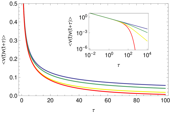
Figure 4: Main figure. Comparison of the velocity autocorrelation functions, from top to bottom: untruncated motion, equation (6) (blue line), weak power-law truncation, equation (13) with $\mu=0.3$ (green line), strong power-law truncation, equation (13) with $\mu=1$ (yellow line), and exponential truncation, equation (10) (red line). Parameters: $H=3/4$, $D_{H}=1$, and $\tau_{\star}=50$. Inset: double-logarithmic representation.

3 Tempered subdiffusive generalised Langevin equation motion

We now consider the motion encoded in the overdamped generalised Langevin equation for a particle with mass $m$ moving in a viscous medium characterised by the friction kernel $\gamma_{H}(t)$ of dimension $[\gamma_{H}(t)]=\mathrm{s}^{-2}$ [7, 38, 45]

$$m\int_{0}^{t}\gamma_{H}(t-t^{\prime})\frac{dx(t^{\prime})}{dt^{\prime}}dt^{\prime}=\xi(t),$$ (22)

where $x(0)=0$ without loss of generality. Similar to the model considered in section 2 $\xi(t)$ is a Gaussian noise with power-law correlation of the form (6) with $1/2\leq H<1$. However, in contrast to the fractional Brownian motion model considered above, we require the system to be thermalised, such that the random force is coupled to the friction kernel through the Kubo-Zwanzig fluctuations dissipation relation [38, 45]

$$\langle\xi^{2}\rangle_{\tau}=k_{B}Tm\gamma_{H}(\tau).$$ (23)

3.1 Mean squared displacement

Let us recall the derivation of the MSD from equations (22) and (23). With our choice $x(0)=0$ we obtain for the Laplace transform of $x(t)$, $\tilde{x}(s)=\int_{0}^{\infty}x(t)\exp(-st)dt$ that

$$\tilde{x}(s)=\frac{\tilde{\xi}(s)}{ms\tilde{\gamma}_{H}(s)}.$$ (24)

Inverse Laplace transformation produces

$$x(t)=\frac{1}{m}\int_{0}^{t}\xi(t^{\prime})H(t-t^{\prime})dt^{\prime},$$ (25)

where the kernel $H(t)$ is the inverse Laplace transform of $\tilde{H}(s)=1/[s\tilde{\gamma}_{H}(s)]$. After some transformation we recover the MSD

$$\langle x^{2}(t)\rangle = \frac{2}{m^{2}}\int_{0}^{t}dt_{1}\int_{t_{1}}^{t}dt_{2}H(t-t_{1})H(t-t_{2})\langle\xi^{2}\rangle_{t_{2}-t_{1}}$$ (26)

$$= \frac{2k_{B}T}{m}\int_{0}^{t}H(t^{\prime})M(t^{\prime})dt^{\prime},$$

where we introduced $M(t)=\int_{0}^{t}\gamma_{H}(t^{\prime})H(t-t^{\prime})dt^{\prime}$. Its Laplace transform is $\tilde{M}(s)=\tilde{\gamma}_{H}(s)\tilde{H}(s)=1/s$, and thus simply $M(t)=1$. We therefore arrive at

$$\langle x^{2}(t)\rangle=\frac{2k_{B}T}{m}\int_{0}^{t}H(t^{\prime})dt^{\prime}.$$ (27)

In Laplace space, this relation reads

$$\langle\tilde{x^{2}}(s)\rangle=\frac{2k_{B}T}{m}\frac{\tilde{H}(s)}{s}=\frac{2k_{B}T}{m}\frac{1}{s^{2}\tilde{\gamma}_{H}(s)}.$$ (28)

We stop to include a note on when exactly we expect asymptotically normal diffusion in the generalised Langevin equation model. The reasoning is similar to that presented at the beginning of section 2. Namely, from equation (28) it follows that diffusion is normal at long times if $\tilde{\gamma}_{H}(s)$ tends to a constant in the limit $s\to 0$. This is equivalent to requiring that the average $\int_{0}^{\infty}\gamma_{H}(\tau)d\tau$ is finite or, taking into account the fluctuation-dissipation relation (23) that $\int_{0}^{\infty}\langle\xi^{2}\rangle_{\tau}d\tau$ is finite (similar to the conclusion in section 2). Then, from expression (28) we infer the following behaviour in the long time limit (compare with equation (5))

$$\langle x^{2}(t)\rangle=\frac{2k_{B}T}{m\int_{0}^{\infty}\gamma_{H}(\tau)d\tau}t.$$ (29)

According to this, anomalous diffusion is expected at long times whenever $\int_{0}^{\infty}\gamma_{H}(\tau)d\tau$ is either infinite (subdiffusion) or zero (superdiffusion).

In accordance with section 2 we choose the friction kernel in the power-law form

$$\gamma_{H}(\tau)=\frac{\Gamma_{H}}{\Gamma(2H-1)}\tau^{2H-2},$$ (30)

where the coefficient $\Gamma_{H}$ is of dimension $[\Gamma_{H}]=\mathrm{s}^{-2H}$. The normal Brownian case is recovered from equation (22) for $H=1/2$ since for $H\to 1/2+$ we see that $\gamma_{H}(t)\to\Gamma_{1/2}\delta(t)$ (note that in this Brownian limit, $\Gamma_{1/2}=\eta$) and equation (22) assumes the form of the standard Langevin equation driven by white Gaussian noise obeying the regular fluctuation dissipation theorem. We note that the memory kernel for the power-law form (30) can be rewritten in terms of a fractional derivative, and the resulting version of equation (22) is then often referred to as the fractional Langevin equation [7, 46, 47, 48]. Power-law memory kernels of the form (30) are typical for many viscoelastic systems [8, 9, 14, 15, 16, 17, 19, 20, 22, 48].

We now use the Laplace transform of equation (30), $\tilde{\gamma}_{H}(s)=\Gamma_{H}s^{1-2H}$, plug this into the above expression, and take an inverse Laplace transformation. This procedure leads to the final result

$$\langle x^{2}(t)\rangle=\frac{1}{\Gamma(3-2H)}\frac{2k_{B}T}{m\Gamma_{H}}t^{2-2H},$$ (31)

which reduces to the classical result $\langle x^{2}(t)\rangle=2(k_{B}T/[m\eta])t$ for normal Brownian motion in the limit $H=1/2$. Therefore, due to the requirement that the system is thermalised and thus the Kubo-Zwanzig fluctuation theorem is fulfilled, the same noise leads to subdiffusion in this case with anomalous diffusion exponent $\alpha=2-2H$ and $0<2-2H<1$. Indeed, due to the coupling in relation (23) large noise values lead to large friction values, and therefore the persistence of the noise is turned into antipersistent diffusion dynamics [7, 46, 48].

3.2 Autocorrelation functions of displacements and velocities

We now derive the autocorrelation function of the displacements, following the procedure laid out by Pottier [49]. First, we note that the double Laplace transform of the correlation function of the random force can be written as

$$\langle\tilde{\xi}(s_{1})\tilde{\xi}(s_{2})\rangle=k_{B}Tm\int_{0}^{\infty}dt_{1}\int_{0}^{\infty}dt_{2}e^{-s_{1}t_{1}-s_{2}t_{2}}\gamma_{H}(|t_{2}-t_{1}|).$$ (32)

Then we split the domain of integration over $t_{2}$ into the two domains $0\leq t_{2}\leq t_{1}$ and $t_{1}\leq t_{2}<\infty$. After introducing $\tau=t_{1}-t_{2}$ and $\tau=t_{2}-t_{1}$ in each domain, respectively, we arrive at

$$\langle\tilde{\xi}(s_{1})\tilde{\xi}(s_{2})\rangle=k_{B}Tm\frac{\tilde{\gamma}_{H}(s_{1})+\tilde{\gamma}_{H}(s_{2})}{s_{1}+s_{2}}.$$ (33)

This expression represents the Laplace domain formulation of the fluctuation dissipation theorem (23). By help of equations (33) and (22) we then obtain the double Laplace transform of the displacement correlation function,

$$\langle\tilde{x}(s_{1})\tilde{x}(s_{2})\rangle=\frac{k_{B}T}{m}\left(\frac{1/\tilde{\gamma}_{H}(s_{1})}{s_{1}s_{2}(s_{1}+s_{2})}+\frac{1/\tilde{\gamma}_{H}(s_{2})}{s_{1}s_{2}(s_{1}+s_{2})}\right).$$ (34)

In the first term in the parentheses we first take the inverse Laplace transformation over $s_{2}$, going from $1/[s_{2}(s_{1}+s_{2})]$ to $[1-\exp(-s_{1}t_{2})]/s_{1}$. Exchanging $s_{2}$ for $s_{1}$ we perform the same operation on the second term. Then we inverse Laplace transform the first term with respect to $s_{1}$ and make use of the translation formula $\mathscr{L}_{s}^{-1}\left\{\exp(-bs)\mathscr{L}_{s}\left\{f(t)\right\}\right\}=f(t-b)\Theta(t-b)$, where $b>0$ and $\Theta(t)$ is the Heaviside step function. As result yields

$$\langle x(t_{1})x(t_{2})\rangle=\frac{1}{\Gamma(3-2H)}\frac{k_{B}T}{m\Gamma_{H}}\Big{(}t_{1}^{2-2H}+t_{2}^{2-2H}-|t_{2}-t_{1}|^{2-2H}\Big{)}.$$ (35)

The velocity autocorrelation function is obtained by differentiation of this expression,

$$\langle v(t_{1})v(t_{2})\rangle=\langle v^{2}\rangle_{\tau}=-\frac{\sin(\pi[2H-1])\Gamma(2H)}{\pi}\frac{k_{B}T}{m\Gamma_{H}}|\tau|^{-2H},$$ (36)

where $\tau=t_{2}-t_{1}$. We see that in the relevant parameter range $1/2<H<1$ the velocity autocorrelation is negative, $\langle v^{2}\rangle_{\tau}<0$, reflecting the antipersistent character of the resulting motion.

3.3 Exponentially truncated fractional Gaussian noise

For the exponentially truncated friction kernel and thus noise autocorrelation

$$\gamma_{H}(\tau)=\frac{\langle\xi^{2}\rangle_{\tau}}{k_{B}Tm}=\frac{\Gamma_{H}}{\Gamma(2H-1)}\tau^{2H-2}e^{-\tau/\tau_{\star}}$$ (37)

we obtain the corresponding Laplace transform

$$\tilde{\gamma}_{H}(s)=\Gamma_{H}\left(s+\tau_{\star}^{-1}\right)^{1-2H}.$$ (38)

After plugging this expression into relation (28) and taking the inverse Laplace transformation we obtain

$$\langle x^{2}(t)\rangle=\frac{2k_{B}T}{m\Gamma_{H}}t^{2-2H}E_{1,3-2H}^{1-2H}\left(-\frac{t}{\tau_{\star}}\right)$$ (39)

in terms of the three parameter Mittag-Leffler function $E_{\alpha,\beta}^{\delta}(z)$ (see B for its definition and some relevant properties). When the crossover time $\tau_{\star}$ tends to infinity, $E_{\alpha,\beta}^{\delta}(0)=1/\Gamma(\beta)$, and we arrive at result (31) for the untruncated noise. In the limit $H=1/2$ we have $\delta=0$ and $E_{1,2}^{0}(z)=1/\Gamma(2)=1$, such that equation (39) reduces to the MSD of normal Brownian motion.

At short times $t\ll\tau_{\star}$ the MSD (39) reduces to the subdiffusive expression (31), whereas at long times $t\gg\tau_{\star}$ with the help of $E_{1,3-2H}^{1-2H}(-t/\tau_{\star})\sim(t/\tau_{\star})^{2H-1}$ (see A), in accordance with relation (29) the MSD exhibits normal Brownian behaviour,

$$\langle x^{2}(t)\rangle\sim\frac{2k_{B}T}{m\Gamma_{H}\tau_{\star}^{2H-1}}t.$$ (40)

We note that a similar crossover was observed in [50] where a modified three-parameter Mittag-Leffler form for the kernel $\gamma_{H}(\tau)$ was considered.

The crossover from subdiffusion to normal diffusion in this exponentially tempered generalised Langevin equation picture is shown in figure 5. The crossover behaviour occurs over an interval of the order of a decade in time for the chosen parameters.

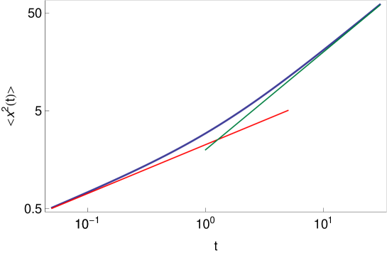
Figure 5: MSD (39) for exponentially tempered generalised Langevin equation motion with $H=3/4$, $k_{B}T/[m\Gamma_{H}]=1$, and $\tau_{\star}=1$ (blue line). The short and long time asymptotics (31) and (40) are shown by the red and green lines, respectively.

Let us now turn to the autocorrelation functions. Using expression (38) in equation (34) we obtain

$$\langle\tilde{x}(s_{1})\tilde{x}(s_{2})\rangle=\frac{k_{B}T}{m\Gamma_{H}} \left(\frac{1}{s_{1}s_{2}(s_{1}+s_{2})\left(s_{1}+\tau_{\star}^{-1}\right)^{1-2H}}\right.$$ (41)

$$\left.+\frac{1}{s_{1}s_{2}(s_{1}+s_{2})\left(s_{2}+\tau_{\star}^{-1}\right)^{1-2H}}\right).$$

As above, in the first term in the parentheses we take an inverse Laplace transformation with respect to $s_{2}$, and over $s_{1}$ in the second term. Then, with the translation formula and the Laplace transform (101) of the three parameter Mittag-Leffler function, we find

$$\langle x(t_{1})x(t_{2})\rangle=\frac{k_{B}T}{m\Gamma_{H}} \left(t_{1}^{2-2H}E_{1,3-2H}^{1-2H}\left(-\frac{t_{1}}{\tau_{\star}}\right)+t_{2}^{2-2H}E_{1,3-2H}^{1-2H}\left(-\frac{t_{2}}{\tau_{\star}}\right)\right.$$ (42)

$$\left.-|t_{2}-t_{1}|^{2-2H}E_{1,3-2H}^{1-2H}\left(-\frac{|t_{2}-t_{1}|}{\tau_{\star}}\right)\right).$$

Differentiation over $t_{1}$ and $t_{2}$ (with the help of equation (105)) then produces the velocity autocorrelation function,

$$\langle v(t_{1})v(t_{2})\rangle=\langle v^{2}\rangle_{\tau}=\frac{k_{B}T}{m\Gamma_{H}\tau^{2H}}E_{1,1-2H}^{1-2H}\left(-\frac{\tau}{\tau_{\star}}\right).$$ (43)

with $\tau=t_{2}-t_{1}>0$. Using the definition (100) of the three parameter Mittag-Leffler function it is easy to check that $E_{1,\delta}^{\delta}(z)=\exp(z)/\Gamma(\delta)$. Thus, for the velocity autocorrelation function we find the result

$$\langle v^{2}\rangle_{\tau}=-\frac{\sin(\pi[2H-1])\Gamma(2H)}{\pi}\frac{k_{B}T}{m\Gamma_{H}}\tau^{-2H}e^{-\tau/\tau_{\star}},$$ (44)

which is anticorrelated and reduces to the untruncated result (36) when the crossover time $\tau_{\star}$ tends to infinity.

3.4 Power-law truncated fractional noise

For the power-law truncated friction kernel and noise autocorrelator,

$$\gamma_{H}(\tau)=\frac{\langle\xi^{2}\rangle_{\tau}}{k_{B}Tm}=\frac{\Gamma_{H}}{\Gamma(2H-1)}\tau^{2H-2}\left(1+\frac{\tau}{\tau_{\star}}\right)^{-\mu}$$ (45)

with $\tau>0$, $\mu>0$ the Laplace transform of the memory kernel can be performed by use of the integral representation of the Tricomi hypergeometric function $U(a,b;z)$ (see 13.2.5 of [42]), leading to

$$\tilde{\gamma}_{H}(s)=\Gamma_{H}\tau_{\star}^{2H-1}U(2H-1,2H-\mu;s\tau_{\star}).$$ (46)

With the general relation (28) we thus have

$$\langle x^{2}(t)\rangle=\frac{2k_{B}T}{m\Gamma_{H}\tau_{\star}^{2H-1}}g(t)$$ (47)

with the abbreviation

$$g(t)=\mathscr{L}^{-1}_{s}\left\{\frac{1}{s^{2}U(2H-1,2H-\mu;s\tau_{\star})}\right\}.$$ (48)

The inverse Laplace transform of expression (47) cannot be performed analytically. However, we make use of the Tauberian theorems to find the MSD at short and long times.

At short times with $s\tau_{\star}\gg 1$ we use the large argument asymptotic of the Tricomi function, $U(2H-1,2H-\mu;s\tau_{\star})\sim(s\tau_{\star})^{1-2H}$ (13.5.2 in [42]) and thus $\tilde{\gamma}_{H}(s)\sim\Gamma_{H}s^{1-2H}$. From equation (28) (or, equivalently, equations (47) and (48)) we then get to result (31) by use of the Tauberian theorem.

Similar to the case considered in section 2 at long times corresponding to $s\tau_{\star}\ll 1$ the situation is actually richer than for the case of exponential tempering. To see this we first make use of (13.1.3) in [42] to express the Tricomi function via the Kummer function $M(a,b;z)$ through

$$U(2H-1,2H-\mu;s\tau_{\star}) = \frac{\pi}{\sin(\pi[2H-\mu])}\left[\frac{M(2H-1,2H-\mu;s\tau_{\star})}{\Gamma(\mu)\Gamma(2H-\mu)}\right.$$ (49)

$$\left.-(s\tau_{\star})^{\mu+1-2H}\frac{M(\mu,\mu+2-2H;s\tau_{\star})}{\Gamma(2H-1)\Gamma(\mu+2-2H)}\right].$$

Taking into account the series expansion of the Kummer function ((13.1.2) in [42]) we consider the following two possibilities:

3.4.1 Weak power-law truncation, $0<\mu<2H-1<1$.

In this case the second term in (49) is dominant at small $s$ and thus

$$U(2H-1,2H-\mu;s\tau_{\star})\sim\frac{\pi(s\tau_{\star})^{1+\mu-2H}}{\sin(\pi[2H-\mu-1])\Gamma(2H-1)\Gamma(\mu+2-2H)}.$$ (50)

Plugging this leading behaviour into expressions (47) and (48) and using the Tauberian theorem, after few transformations we obtain the long time behaviour of the MSD,

$$\langle x^{2}(t)\rangle\sim\frac{\Gamma(2H-1)}{\Gamma(2H-\mu-1)\Gamma(\mu+3-2H)}\frac{2k_{B}T}{m\Gamma_{H}\tau_{\star}^{\mu}}t^{\mu+2-2H}.$$ (51)

Note that in the limit $\mu\to 0$ expression (51) reduces to the untruncated formula (31). Thus, since we observe the inequality $0<\mu+2-2H<1$ in the present case of a weak power-law truncation, the dynamics is still subdiffusive, however, with an anomalous diffusion exponent larger than the value $2-2H$ in the short time limit.

3.4.2 Strong power-law truncation, $\mu>2H-1>0$.

In this case the first term in the square brackets in equation (49) becomes dominant at small $s$ and $U(2H-1,2H-\mu;s\tau_{\star})\sim\Gamma(\mu+1-2H)/\Gamma(\mu)$, where we made us of the reflection formula for the Gamma function. From results (47) and (48) by use of the Tauberian theorem we obtain

$$\langle x^{2}(t)\rangle\sim\frac{\Gamma(\mu)}{\Gamma(\mu+1-2H)}\frac{2k_{B}T}{m\Gamma_{H}\tau_{\star}^{2H-1}}t,$$ (52)

valid for $t\gg\tau_{\star}$. As expected, we find the desired crossover to the normal Brownian scaling of the MSD. Note that this result is in full accordance with equation (29). Indeed, from expression (45) we get (see 2.2.5.24 [62])

$$\int_{0}^{\infty}\gamma_{H}(\tau)d\tau=\frac{\Gamma(\mu+1-2H)}{\Gamma(\mu)}\Gamma_{H}\tau_{\star}^{2H-1}.$$ (53)

After plugging expression (53) into (29) we arrive at result (52). Note also that the condition of a strong power-law truncation is equivalent to the condition that integral (53) converges.

In the borderline case with $0<\mu=2H-1<1$ we use 13.5.9 in [42] and find $U(2H-1,1;s\tau_{\star})\sim-\ln(s\tau_{\star})/\Gamma(2H-1)$. With the use of the Tauberian theorem equations (47) and (48) yield

$$\langle x^{2}(t)\rangle\sim\Gamma(2H-1)\frac{2k_{B}T}{m\Gamma_{H}\tau_{\star}^{2H-1}}\frac{t}{\ln(t/\tau_{\star})}$$ (54)

at $t\gg\tau_{\star}$. Thus, in this borderline situation between the cases of weak truncation (leading to increased subdiffusion at long times) and strong truncation (normal long time diffusion) we observe a logarithmic correlation to normal diffusion.

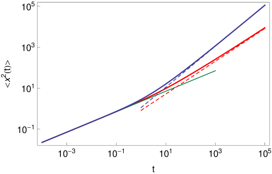
Figure 6: MSD (47) for power-law truncation with $H=3/4$, $k_{B}T/[m\Gamma_{H}]=1$, and $\tau_{\star}=1$. The red solid line corresponds to weak power-law truncation with $\mu=0.3$, the blue solid line to strong truncation with $\mu=1$. The asymptotics (51) and (52) are shown by red and blue dashed lines, respectively. The thin green solid line corresponds to the MSD (31) for the untruncated case.

Figure 6 shows the crossover dynamics for power-law tempering for the two possible cases: for weak power-law truncation with $\mu=0.3$ we observe the predicted crossover from slower to faster subdiffusion, while in the case of strong power-law truncation the subdiffusive dynamics crosses over to normal diffusion.

Figure 7 shows a direct comparison between the cases of exponential and power-law truncation. As expected, the crossover is faster for the exponential tempering, and thus the resulting amplitude in this case exceeds the amplitude for the power-law tempering. Note that the latter observation contrasts the case of the truncated fractional Brownian motion in figure 3, for which the amplitude of the power-law tempering is higher.

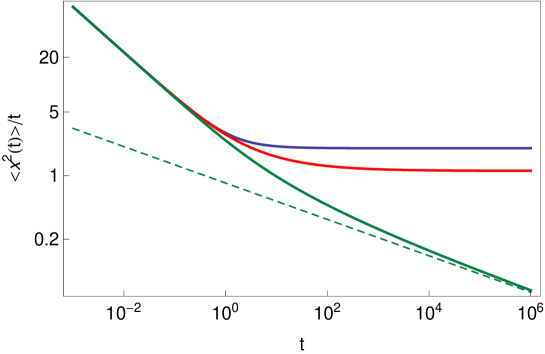
Figure 7: Comparison of the ratio $\langle x^{2}\rangle/t$ for different truncation modes of the power-law noise in the generalised Langevin equation (22). Parameters: $H=3/4$, $k_{B}T/[m\Gamma_{H}]=1$, and $\tau_{\star}=1$. From top to bottom the blue line represents the exponential truncation, equation (39), the red line the strong power-law truncation, equation (47) with $\mu=1$, and the green line the weak power-law truncation, equation (47) with $\mu=0.3$. The asymptotics (51) is shown by dashed green line.

3.4.3 Velocity autocorrelation function.

To gain some insight into the correlation behaviour we use equation (34) with $\tilde{\gamma}_{H}(s)$ from equation (46). Taking the inverse Laplace transformation over $s_{1}$ and $s_{2}$ in the same way as above we obtain the position autocorrelation function

$$\langle x(t_{1})x(t_{2})\rangle=\frac{k_{B}T}{m\Gamma_{H}\tau_{\star}^{2H-1}}\Big{(}g(t_{1})+g(t_{2})-g(|t_{2}-t_{1}|)\Big{)},$$ (55)

where $g(t)$ is given by relation (48). From here the velocity autocorrelation function is obtained as

$$\langle v^{2}\rangle_{\tau}=\frac{k_{B}T}{m\Gamma_{H}\tau_{\star}^{2H-1}}\frac{d^{2}}{d\tau^{2}}g(\tau)$$ (56)

with $\tau>0$. We first note that expression (56) along with (48) may suggest that the Tauberian theorem may be directly applied to the expression $U^{-1}(2H-1,2H-\mu;s\tau_{\star})$ in order to calculate the asymptotic behaviour of the velocity autocorrelation function $\langle v^{2}\rangle_{\tau}$. However, for short times corresponding to $s\tau_{\star}\gg 1$ the function $U^{-1}\sim(s\tau_{\star})^{2H-1}$, and since $1/2<H<1$, the Tauberian theorem does not apply as $2H-1$ is positive. Instead, we should first obtain the asymptotic of $g(\tau)$ at short times $\tau\ll\tau_{\star}$ by use of the Tauberian theorem, and only then differentiate twice to get the asymptotic of the velocity autocorrelation function. This way we arrive at expression (36). At long times $\tau\gg\tau_{\star}$ we again consider the cases of weak and strong power-law truncations separately.

For the weak power-law truncation with $0<\mu<2H-1<1$ the situation is similar to the short time limit above. Indeed, $U^{-1}\sim(s\tau_{\star})^{2H-1-\mu}$, see result (50), and the Tauberian theorem does not apply. Instead we first plug relation (50) into expression (48) and then apply the Tauberian theorem. Following relation (56) we then find

$$\langle v^{2}\rangle_{\tau}\sim-C\frac{k_{B}T}{m\Gamma_{H}\tau_{\star}^{\mu}}\frac{1}{\tau^{2H-\mu}},$$ (57)

where $C=(2H-\mu-1)\pi^{-1}\sin(\pi[2H-\mu-1])\Gamma(2H-1)$ is a positive constant. Note that for weak power-law truncation we have $1<2H-\mu<2$, and in the limit $\mu\to 0$ expression (57) reduces to the velocity autocorrelation function (36) in absence of truncation. From comparison of result (57) with (36) we see that the autocorrelation function in the truncated case decays slower than in the untruncated case. This may appear counter-intuitive, however, it is in agreement with the antipersistent character of the fractional Langevin equation model in which the MSD scales like $\simeq t^{2-2H}$ and the velocity autocorrelation function at long times scales as $\simeq-\tau^{-2H}$ for $1/2<H<1$. This means that a steeper decay of the velocity autocorrelation function corresponds to a more subdiffusive regime. In other words, when $H$ is closer to $1/2$ (the subdiffusive regime is closer to normal diffusion) then the decay of the autocorrelation function is slower. To see this better consider the effective Hurst index $H_{\mathrm{eff}}=H-\mu/2$. Then, for weak power-law truncation the MSD scales like $\simeq t^{2-2H_{\mathrm{eff}}}$ with $1/2<H_{\mathrm{eff}}<H<1$, and the velocity autocorrelation function decays as $\simeq-\tau^{-}{2H_{\mathrm{eff}}}$. Thus, in the truncated case the diffusion becomes closer to normal, as it should be, while the velocity autocorrelation function decays slower than in the untruncated case, fully consistent with the antipersistent fractional Langevin equation model.

Now let us turn to the case of strong power-law truncation with $\mu>2H-1>0$ in which for simplicity we assume that $\mu+1-2H\neq n$ where $n\in\mathbb{N}$ is a positive integer. We are interested in the exponent of the power-law decay of the velocity autocorrelation function. Then expression (49) yields $U(2H-1,2H-\mu;s\tau_{\star})\sim a_{0}+a_{1}s+a_{2}s^{2}+\ldots a_{k}s^{k}+a_{\mu}s^{\mu+1-2H}+a_{k+1}s^{k+1}+\ldots$, where $a_{i}$ with $i=0,1,2,\ldots$ are constants that can be easily found from expansion 13.1.2 in [42] for the first Kummer function in the square brackets of expression (49) and $k=[\mu+1-2H]$ denotes the integer part of the corresponding argument in the Landau bracket $[\cdot]$. Then $U^{-1}(2H-1,2H-\mu;s\tau_{\star})\sim b_{0}+b_{1}s+\ldots+b_{k}s^{k}+b_{\mu}s^{\mu+1-2H}+\ldots$ where the $b_{i}$ with $i=0,1,2,\ldots$ are again constant factors. From here and with equations (48) and (56) we find after application of the Tauberian theorem and subsequent double differentiation

$$\langle v^{2}\rangle_{\tau}\sim-C\frac{k_{B}T}{m\Gamma_{H}\tau_{\star}^{2H-1}}\frac{1}{\tau^{\mu+2-2H}},$$ (58)

where $C$ is a positive constant. Note that in the borderline case $1>\mu=2H-1>0$ both expressions (57) and (58) tend to the same limit resulting in the logarithmic correction to normal diffusion in expression (54).

A graphical representation of the velocity autocorrelation function (36), (44) and (58) is shown in figure 8.

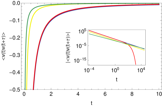
Figure 8: Comparison of the velocity autocorrelation functions for the untruncated case, equation (36) (blue line), with exponential truncation, equation (44) (red line), and with strong power-law truncation, equation (58) where $\mu=1$ (yellow line), as well as with weak power-law truncation, equation (57) where $\mu=0.3$ (green line). Parameters: $H=3/4$, $k_{B}T/[m\Gamma_{H}]=1$, and $\tau_{\star}=50$.

3.5 Application to lipid molecule dynamics in lipid bilayer membranes

We here demonstrate the usefulness of our tempered fractional Gaussian noise approach to a concrete physical system. The data we have in mind are from all-atom Molecular Dynamics simulations of lipid bilayer membranes [30]. In their simplest form, these are double layered leaves made up of relatively short amphiphilic polymers called lipids. Immersed in water the double layer arrangement prevents the exposure of the hydrophobic tail groups to the ambient water, while the hydrophilic head groups are in contact with the water. At room temperature the lipid bilayer assumes a quite disordered liquid structure [30]. In this lipid matrix, comparatively large membrane proteins may be additionally embedded [30]. Natural biological membranes are composed of lipids of many different chemistries, and they are crowded with membrane proteins. Supercomputing studies have the task to reveal the dynamics of both proteins and lipids in such protein-decorated bilayer systems. This thermally driven diffusion of the constituents influence biological properties of the bilayer, such as diffusion limited aggregation, domain formation, or the membrane penetration by nanoparticles [30].

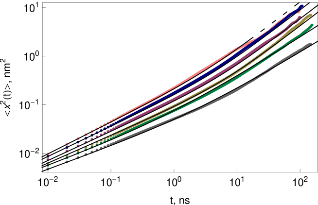
Figure 9: MSD of the motion of lipid molecules in a lipid bilayer model membrane, at room temperature in the liquid disordered and liquid ordered phases (symbols) [22]. The crossover from subdiffusion to normal diffusion or increased subdiffusion at around 10 nsec is distinct. Data courtesy Matti Javanainen, University of Helsinki. The black solid lines provide a fit with equations (39) and (47) resulting from our generalised Langevin equation model with exponentially and power-law truncated noise, respectively. The parameters are presented in Table 1, see also discussion in the text.

Figure 9 depicts the simulations results in a chemically uniform, liquid disordered lipid bilayer membrane as well as in the liquid ordered state in the presence of cholesterol molecules—the system is specified in detail in [22]. The motion of the lipids is Gaussian for all cases and best described as viscoelastic diffusion governed by the generalised Langevin equation (22) fuelled by power-law noise [22, 24, 25]. As can be seen in figure 9 the MSD of the liquid disordered lipid systems exhibits a clear crossover from subdiffusion to normal diffusion at roughly 10 nsec, the typical crossover time scale discussed in literature, at which two nearest neighbour lipid molecules exchange their mutual positions and thus decorrelate their motion [22, 30, 31]. For the liquid ordered cases, one lipid chemistry also shows a subdiffusive-normal crossover, while the two other lipid chemistries lead to a crossover from slower to faster subdiffusion [22]. From fit of the parameters (see the summary in table 1) to the data we observe an excellent agreement with the short and long time scaling regimes and, remarkably, the model fully describes the crossover behaviours without further tuning for both liquid disordered and ordered situations. We note that subdiffusive-diffusive crossovers are also observed for protein-crowded membranes [24, 23, 55].

	$H$	$\mu$	$\tau_{\star}$	$k_{B}T/[m\Gamma_{H}]$	$\alpha_{\mathrm{short}}$	$K_{\alpha_{\mathrm{short}}}$	$\alpha_{\mathrm{long}}$	$K_{\alpha_{\mathrm{long}}}$
			$[\mathrm{nsec}]$	$[\mathrm{nm}^{2}/\mathrm{nsec}^{2-2H}]$		$[\mathrm{nm}^{2}/\mathrm{nsec}^{2-2H}]$		$[\mathrm{nm}^{2}/\mathrm{nsec}^{\alpha_{\mathrm{long}}}]$
DSPC (purple)	0.70	$-$	4.0	0.050	0.60	0.034	1.0	0.029
SOPC (pink)	0.67	$-$	2.5	0.88	0.66	0.064	1.0	0.064
DOPC (blue)	0.69	$-$	3.0	0.067	0.62	0.046	1.0	0.044
DSPC (grey)	0.76	0.41	0.60	0.019	0.48	0.010	0.89	0.0035
SOPC (green)	0.75	0.44	0.22	0.025	0.50	0.014	0.94	0.0026
DOPC (brown)	0.72	$-$	4.3	0.038	0.57	0.024	1.0	0.021

Table 1: Fit parameters for the model membrane simulations data shown in figure 9. The colours mentioned in the first column correspond to the colour coding in figure 9.

We note that from equation (31) and the effective diffusion coefficient

$$K^{*}_{\alpha}(t)=\frac{1}{2}\frac{d}{dt}\left\langle x^{2}(t)\right\rangle.$$ (59)

we find the short time limiting behaviour

$$K^{*}_{\alpha}(t)=K^{*}_{\alpha,\mathrm{short}}t^{1-2H}$$ (60)

with

$$K^{*}_{\alpha,\mathrm{short}}=\frac{k_{B}T}{m\Gamma_{H}}\frac{1}{\Gamma(2-2H)}.$$ (61)

For the long time limit, from equation (40), it follows that

$$K^{*}_{\alpha,\mathrm{long}}=\frac{k_{B}T}{m\Gamma_{H}}\frac{1}{\tau_{\star}^{2H-1}}$$ (62)

for the exponential tempering, whereas the cases of DSPC and SOPC lipid chemistries the long time limit in the weak power-law truncation case is given by

$$K^{*}_{\alpha,\mathrm{long}}=\frac{\Gamma(2H-1)}{\Gamma(2H-\mu+1)\Gamma(\mu+2-2H)}\frac{k_{B}T}{m\Gamma_{H}\tau_{\star}^{\mu}}$$ (63)

The fit values given in table 1 are in very good agreement with those obtained in the simulations study [22]. We note, however, that for the weak power-law tempering model fit the crossover time is somewhat underestimated.

4 Direct tempering of Mandelbrot’s fractional Brownian motion

So far we introduced the tempering on the level of the noise $\xi(t)$, which drives the position co-ordinate $x(t)$. Another way to introduce the crossover from anomalous to normal diffusion is to consider a truncation of the power-law correlations directly in the original definition of fractional Brownian motion according to Mandelbrot and van Ness [36]. Such a formulation was recently proposed by Meerschaert and Sabzikar [56]. Here we analyse this model and demonstrate that it leads to a very different behaviour of the MSD than the previous tempered fractional models. A formal mathematical analysis of this model was provided very recently in [57]. We here recall some of their results for the convenience of the reader and present clear physical arguments for the seemingly paradoxical behaviour of this model. In particular we come up with a comparison to a fractional Ornstein-Uhlenbeck scenario.

4.1 Meerschaert and Sabzikar direct tempering model

Meerschaert and Sabzikar defined this extension of fractional Brownian motion by applying an exponential truncating in Mandelbrot’s definition [36, 56],

$$B_{H,\lambda}(t) = \int_{-\infty}^{0}\left[e^{-\lambda(t-t^{\prime})}(t-t^{\prime})^{H-\frac{1}{2}}-e^{-\lambda(-t^{\prime})}(-t^{\prime})^{H-\frac{1}{2}}\right]B^{\prime}(t^{\prime})dt^{\prime}$$ (64)

$$+\int_{0}^{t}\left[e^{-\lambda(t-t^{\prime})}(t-t^{\prime})^{H-\frac{1}{2}}\right]B^{\prime}(t^{\prime})dt^{\prime},$$

where $H,\lambda,t>0$. $B^{\prime}(t)$ is white Gaussian noise of $\delta$-covariance $\left\langle B^{\prime}(t_{1})B^{\prime}(t_{2})\right\rangle=\sigma^{2}\delta(t_{1}-t_{2})$ and zero mean. The parameter $\lambda$ stands for the truncation parameter, and classical fractional Brownian motion is then obtained in the limiting case $\lambda\to 0$ when $H\in(0,1)$. It should be noted that the prefactor $1/\Gamma(H+1/2)$ in Mandelbrot’s original definition is dropped here in line with the procedure of [56]. The MSD encoded in equation (64) is (see C for the derivation)

$$\left\langle B^{2}_{H,\lambda}(t)\right\rangle=\sigma^{2}C_{t}^{2}t^{2H},$$ (65)

where the prefactor is

$$C_{t}^{2}=\left[\frac{2\Gamma(2H)}{(2\lambda t)^{2H}}-\frac{2\Gamma(H+1/2)}{\sqrt{\pi}}\frac{K_{H}(|\lambda t|)}{(2\lambda t)^{H}}\right].$$ (66)

$K_{H}(z)$ denotes the modified Bessel function of the second kind, which for small argument $z$ behaves as [42]

$$K_{H}(z)\sim\frac{\Gamma(H)}{2^{1-H}}z^{-H}+\frac{\Gamma(-H)}{2^{1+H}}z^{H}+\frac{\Gamma(H)}{2^{3-H}(1-H)}z^{2-H}$$ (67)

while for large $z$ we have $K_{H}(z)\sim\sqrt{\pi/(2z)}e^{-z}$. The fact that the prefactor $C_{t}^{2}$ is an explicit function of time contrasts the result of standard fractional Brownian motion, and we will readily see the ensuing consequences.

In the short time limit $t\ll\lambda^{-1}$ expression (65) has the compound power-law form

$$\left\langle B_{H,\lambda}^{2}(t)\right\rangle\sim\sigma^{2}\Gamma^{2}(H+1/2)V_{H}t^{2H}+\frac{\sigma^{2}\Gamma(2H)}{2^{1+2H}(H-1)}\lambda^{2-2H}t^{2}$$ (68)

with $V_{H}=1/[\Gamma(2H+1)\sin(\pi H)]$. Thus, the limit $\lambda\to 0$ indeed reduces to the expression for standard fractional Brownian motion. In the long time limit $t\gg\lambda^{-1}$ the MSD of this tempered fractional Brownian motion, remarkably, converges exponentially towards a constant value,

$$\left\langle B_{H,\lambda}^{2}(t)\right\rangle\sim\sigma^{2}\left(\frac{2\Gamma(2H)}{(2\lambda)^{2H}}-\frac{2^{1/2-H}\Gamma(H+1/2)}{\lambda^{H+1/2}}t^{H-1/2}e^{-\lambda t}\right),$$ (69)

a result which is at first surprising. This point will be discussed and compared to the fractional Ornstein-Uhlenbeck process below. The functional behaviour of result (69) is shown in figure 14. We note that if we consider the Langevin equation (2) in combination with the directly tempered noise $B^{\prime}_{H\lambda}(t)$, expression (65) and its limiting behaviours (68) and (69) exactly correspond to the dynamics of the MSD $\langle x^{2}(t)\rangle$.

As shown in [57] it is possible to define a tempered fractional Gaussian noise following Mandelbrot and van Ness’ smoothening procedure involving a short time lag $\delta$ (see C.2). The autocorrelation function of this tempered fractional Gaussian noise is given through

$$\left\langle B_{H,\lambda}^{\prime}(t)B_{H,\lambda}^{\prime}(t+\tau)\right\rangle = \frac{\Gamma(H+\frac{1}{2})\sigma^{2}}{\sqrt{\pi}(2\lambda)^{H}\delta^{2}}\Big{[}2\tau^{H}K_{H}(|\lambda\tau|)-(\tau+\delta)^{H}K_{H}(\lambda|\tau+\delta|)$$ (70)

$$-|\tau-\delta|^{H}K_{H}(\lambda|\tau-\delta|)\Big{]}.$$

An important feature of the autocorrelation function (70) for tempered fractional Gaussian noise is its antipersistent behaviour over the whole range $0<H<1$ for any finite $\lambda$, that is, the integral of expression (70) over the entire domain of $\tau$ vanishes:

$$\int_{0}^{\infty}\left\langle B_{H,\lambda}^{\prime}(t)B_{H,\lambda}^{\prime}(t+\tau)\right\rangle d\tau=0.$$ (71)

This is in sharp contrast to (conventional) fractional Gaussian noise. Indeed, in the limit $\lambda\to 0$ the noise autocorrelation function (70) approaches the one of fractional Gaussian noise [36, 56], as can be derived by using the small argument expansion (67) of the Bessel function. In this limit $\lambda\to 0$ for any finite $\tau$ the autocorrelation function (70) converges to

$$\lim_{\lambda\to 0}\left\langle B_{H,\lambda}^{\prime}(t)B_{H,\lambda}^{\prime}(t+\tau)\right\rangle\sim\frac{\Gamma^{2}(H+\frac{1}{2})\sigma^{2}V_{H}}{2\delta^{2}}\left[(\tau+\delta)^{2H}+|\tau-\delta|^{2H}-2\tau^{2H}\right]$$ (72)

and shows negative correlations for $0<H<1/2$ and positive correlations for $1/2<H<1$, see C.3.

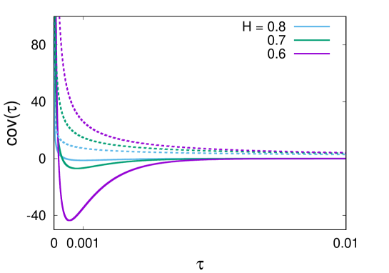
Figure 10: Theoretical results for autocorrelation function, equations (70) and (72), for three different $H>\frac{1}{2}$ values. The solid lines show the antipersistent behaviour of autocorrelation function of tempered fractional Gaussian noise, which approaches zero exponentially; while dashed lines represent the power-law decay of the autocorrelation function of the fractional Gaussian noise. Parameters used: $\lambda=10^{3}$, $\delta=10^{-5}$.

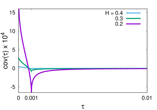
Figure 11: Theoretical results for autocorrelation function, equations (70) and (72), for three different $H<\frac{1}{2}$ values. The solid lines show the autocorrelation function of tempered fractional Gaussian noise and dashed lines are representation of autocorrelation function for fractional Gaussian noise. There is no significant difference between the two functions, except around the truncation time, $\lambda^{-1}$, which is magnified in Fig. (12). Parameters used: $\lambda=10$, $\delta=10^{-3}$.

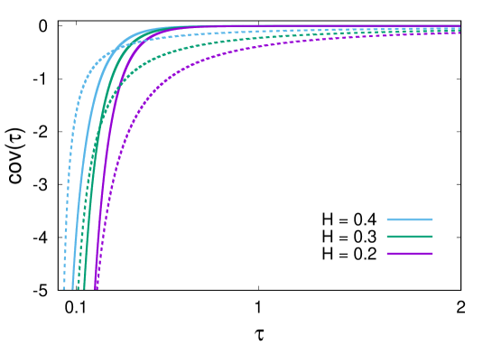
Figure 12: Comparison between the exponentially fast decay of the autocorrelation function of tempered fractional Gaussian noise (solid lines), equation (74), and the slower power-law decay of its ($\lambda\to 0$) regime, which equivalents to fractional Gaussian noise (dashed lines), equation (73), around the truncation time. Parameters used:$\lambda=10$, $\delta=10^{-3}$.

The autocorrelation function (70) and its limit for $\lambda\to 0$ are shown in figures 10 and 11 for different values of the Hurst parameter. While for the tempered process it is antipersistent for the whole range of $H$, in the limit $\lambda\to 0$ we clearly see the difference between the antipersistent case with the overshoot to negative values and a slow recovery back to zero. The autocorrelation function for the persistent case is always positive.

It is easy to show that for $\tau\ll 1/\lambda$ and $\delta\to 0$ the autocorrelation function (70) decays as a power law, consistent with the behaviour of fractional Gaussian noise,

$$\left\langle B_{H,\lambda}^{\prime}(t)B_{H,\lambda}^{\prime}(t+\tau)\right\rangle \sim \sigma^{2}(2H-1)H\Gamma^{2}(H+1/2)V_{H}|\tau|^{2H-2}$$ (73)

$$-\frac{\sigma^{2}\Gamma(2H)\lambda^{2-2H}}{2^{2H+1}(1-H)},$$

while the asymptotic behaviour at long observation times, $\tau\gg\lambda^{-1}$,

$$\left\langle B_{H,\lambda}^{\prime}(t)B_{H,\lambda}^{\prime}(t+\tau)\right\rangle\sim\frac{\tau^{H-\frac{1}{2}}e^{-\lambda\tau}\sigma^{2}}{2^{H-\frac{1}{2}}\lambda^{H+\frac{1}{2}}\delta^{2}}\left[1-\cosh(\lambda\delta)+\sinh(\lambda\delta)\frac{(H-\frac{1}{2})\delta}{\tau}\right]$$ (74)

decays exponentially, in contrast to the non-tempered limit in equation (73). This different asymptotic behaviour of tempered versus non-tempered fractional Gaussian noise around the truncation time, is shown in figure 12.

4.2 Fractional Langevin equation with directly tempered fractional Gaussian noise

Considering the internal noise $\xi(t)$ of the system as the tempered fractional Gaussian noise $B^{\prime}_{H,\lambda}(t)$ defined above, the overdamped tempered fractional Langevin equation reads [57]

$$\int_{0}^{t}\gamma_{H}(t-\tau)\frac{dx}{d\tau}d\tau=\xi(t),$$ (75)

in which $\gamma_{H}(\tau)=2\left\langle B_{H,\lambda}^{\prime}(t)B_{H,\lambda}^{\prime}(t+\tau)\right\rangle$. Similar to our derivation above, we obtain the Laplace transform of the MSD (28) in dimensionless units,

$$\langle\tilde{x}^{2}(s)\rangle=\frac{2}{s^{2}\tilde{\gamma}_{H}(s)},$$ (76)

in which we have to find the Laplace transformation of the autocorrelation function (70). We assume that $\sigma^{2}=1$ for simplicity from now on. To proceed, in the second and third terms we change the variables and split the resulting integrals,

$$\tilde{\gamma}_{H}(s) = \frac{2\Gamma(H+\frac{1}{2})}{\sqrt{\pi}(2\lambda)^{H}\delta^{2}}\left\{2[1-\cosh(\delta s)]\int_{0}^{\infty}dte^{-st}t^{H}K_{H}(\lambda t)\right.$$ (78)

$$+\left.2\int_{0}^{\delta}dt\sinh(s(\delta-t))t^{H}K_{H}(\lambda t)\right\}.$$

First, we expand the above functions up to second order in $\delta$. Since in the second integral $\delta\ll\lambda^{-1}$ and $t<\delta$ the relevant regimes are $\delta s\ll 1$ and $\lambda t\ll 1$. Therefore, to second order in $\delta$, $\tilde{\gamma}_{H}(s)$ is

$$\tilde{\gamma}_{H}(s) \sim \frac{2\Gamma(H+\frac{1}{2})}{\sqrt{\pi}(2\lambda)^{H}\delta^{2}}\left\{2\frac{-(\delta s)^{2}}{2}\int_{0}^{\infty}dte^{-st}t^{H}K_{H}(\lambda t)\right.$$ (79)

$$\left.+2\int_{0}^{\delta}dt(s(\delta-t))t^{H}K_{H}(\lambda t)\right\}.$$

Using expansion (67) and keeping terms up to the second order of $\delta$ we find

$$2\int_{0}^{\delta}dt(s(\delta-t))t^{H}K_{H}(\lambda t)\sim\frac{2^{H}s\pi}{\sin(\pi H)\Gamma(1-H)\lambda^{H}}\frac{\delta^{2}}{2}.$$ (80)

Insertion of this result back to relation (79) yields

$$\tilde{\gamma}_{H}(s)\sim\frac{2\Gamma(H+\frac{1}{2})}{\sqrt{\pi}(2\lambda)^{H}\delta^{2}}\left\{\frac{\pi 2^{H-1}s\delta^{2}}{\sin(\pi H)\Gamma(1-H)\lambda^{H}}-(\delta s)^{2}\int_{0}^{\infty}dte^{-st}t^{H}K_{H}(\lambda t)\right\}.$$ (81)

The integral in (81) is a Laplace transformation, for which we apply equation (2.16.6.3) of [58]. Hence we find the expression for the autocorrelation function in Laplace space,

$$\tilde{\gamma}_{H}(s) \sim \frac{2\Gamma(H+\frac{1}{2})}{\sqrt{\pi}(2\lambda)^{H}\delta^{2}}\left\{\frac{\pi 2^{H-1}s\delta^{2}}{\sin(\pi H)\Gamma(1-H)\lambda^{H}}\right.$$ (82)

$$\left.-(\delta s)^{2}\frac{s^{-1}\lambda^{-H}}{2^{H+1}}\sqrt{\pi}\frac{\Gamma(2H+1)}{\Gamma(H+3/2)}\,_{2}F_{1}\left(\frac{1}{2},1;H+\frac{3}{2};1-\frac{\lambda^{2}}{s^{2}}\right)\right\}$$

in terms of the hypergeometric function ${}_{2}F_{1}$ [42].

4.2.1 Short time behaviour of the MSD

For the regime of short observation times, $\delta\ll t\ll 1/\lambda$ we apply the linear transformations for hypergeometric functions (for more details see (C.4)). Then, with the general definition for hypergeometric functions up to second order and some simplifications, we find the dominant term for the autocorrelation function,

$$\tilde{\gamma}_{H}(s)\sim\frac{2\Gamma^{2}(H+\frac{1}{2})}{2\sin(\pi H)}s^{1-2H}.$$ (83)

Substituting this into expression (76), we see that

$$\langle\tilde{x}^{2}(s)\rangle\sim\frac{2\sin(\pi H)}{2\Gamma^{2}(H+\frac{1}{2})}s^{2H-3}.$$ (84)

By inverse Laplace transformation we find the asymptotic MSD behaviour in time,

$$\langle x^{2}(t)\rangle\sim\frac{\sin(\pi H)}{\Gamma^{2}(H+\frac{1}{2})}\frac{t^{2-2H}}{\Gamma(3-2H)}.$$ (85)

This result corresponds to subdiffusion for $1/2<H<1$ in agreement with the findings in section 3. For $0<H<1/2$ the behaviour is superdiffusive.

4.2.2 Long time behaviour of the MSD

For the long times regime $t\gg 1/\lambda$ or $\lambda/s\gg 1$ we go back to expression (82) and use the same method as in the previous subsection (see also (C.5)). It can be seen that the dominant term is a linear function of $s$,

$$\tilde{\gamma}(s)\sim\frac{\sqrt{\pi}}{2\lambda^{2H}}\frac{2\Gamma(H+\frac{1}{2})}{\sin(\pi H)\Gamma(1-H)}s.$$ (86)

Getting back to equation (76) for the MSD, this yields

$$\langle\tilde{x}^{2}(s)\rangle\sim\frac{2\lambda^{2H}\sin(\pi H)\Gamma(1-H)}{2\Gamma(H+\frac{1}{2})\sqrt{\pi}}s^{-3}.$$ (87)

After inverse Laplace transformation, we obtain

$$\langle x^{2}(t)\rangle\sim\frac{\sin(\pi H)\Gamma(1-H)\lambda^{2H}}{\Gamma(H+\frac{1}{2})\sqrt{\pi}}t^{2}=\frac{\sqrt{\pi}\lambda^{2H}}{\Gamma(H+\frac{1}{2})\Gamma(H)}t^{2}.$$ (88)

Thus, at long times this process converges to ballistic diffusion, as already observed in [57].

The general behaviour of the MSD and its crossover from short time power-law behaviour to long time ballistic motion is shown in figure 13 for different Hurst exponents.

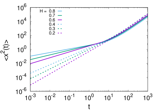
Figure 13: MSD for the tempered Langevin equation (75), from numerical Laplace inversion based on result (82). We also show the transition from anomalous diffusion for short time, equation (85), to the ballistic regime for long observation times, equation (88), is shown for different Hurst exponents and $\lambda=0.1$.

4.3 Physical discussion of the direct tempering model and Ornstein-Uhlenbeck with fractional Gaussian noise

To come back to the above observed finite limiting value at long times, encoded in expression (69), of the MSD in the tempered fractional Brownian process we briefly study the confined fractional Brownian motion in an harmonic potential. Experimentally, such a situation arises, for instance, when particle tracking is performed with an optical tweezers setup in a viscoelastic environment [9, 20]. We thus consider the Ornstein-Uhlenbeck process

$$\frac{dx(t)}{dt}=-\lambda x(t)+B^{\prime}_{H}(t),$$ (89)

for $t>0$ and with $x(0)=0$, where the noise $B^{\prime}_{H}(t)$ is again fractional Gaussian noise. The MSD reads (see D)

$$\langle x^{2}(t)\rangle=\sigma^{2}V_{H}t^{2H}e^{-\lambda t}\left[1+\frac{\lambda t}{4H+2}\left(e^{\lambda t}f_{H}(-\lambda t)-e^{-\lambda t}f_{H}(\lambda t)\right)\right],$$ (90)

where $f_{H}(x)\equiv M(2H+1;2H+2;x)$ is Kummer’s confluent hypergeometric function. For $t\ll\lambda^{-1}$, the MSD of this fractional Ornstein-Uhlenbeck process assumes the form

$$\langle x^{2}(t)\rangle\sim\sigma^{2}V_{H}t^{2H}(1-\lambda t),$$ (91)

which corresponds to unconfined fractional Brownian motion with a correction proportional to $\lambda t$. In the long-time limit an exponentially fast convergence occurs to the stationary limit

$$\langle x^{2}(t)\rangle\sim\frac{\sigma^{2}}{2\sin(\pi H)\lambda^{2H}}.$$ (92)

Figure 14 compares the MSDs of tempered fractional Brownian motion and of the fractional Ornstein-Uhlenbeck process. Both of them saturate at long times, where the plateau value depends on the value of $H$, compare also [59, 60]. Curiously, the plateau values of both processes become identical for the Hurst exponent $H=0.768149$.

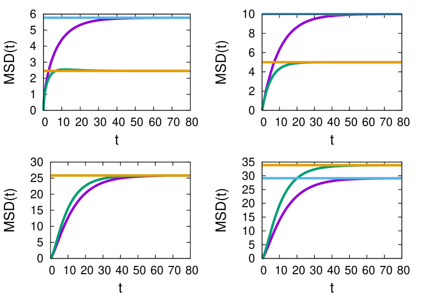
Figure 14: MSD of the tempered fractional Brownian motion (equation (69), violet line) and the fractional Ornstein-Uhlenbeck process (equation (90), green line) and their long time plateaus (horizontal lines) for several values of the Hurst exponent $H$ and the same parameters $\sigma^{2}=1$ and $\lambda=0.1$. Top left: $H=0.3$, top right: $H=0.5$, bottom left: $H=0.768149$ (equivalence of the plateau values), bottom right: $H=0.8$.

From the comparison with this fractional Ornstein-Uhlenbeck process we see that the direct tempering model of Meerschaert and Sabziker actually describes a confined motion, in contrast to the simple intuition of the tempering in equation (64). In that sense it is fundamentally different from the truncated models considered in the previous sections which show a crossover between two regimes of steadily increasing MSD.

The effect of direct tempering for the fractional Langevin equation model, a priori is even more surprising. Namely, as we saw from equations (85) and (88), this model demonstrates a crossover from a short time subdiffusive to a ballistic regime at long times. Such a behaviour appears counterintuitive. However, as we show not, it is actually a simple consequence of the two basic features of the directly tempered internal fractional Gaussian noise (75): (i) the integral of its autocorrelation function over the entire time domain from zero to infinity is identical to zero, see relation (71); (ii) at long times the autocorrelation function exhibits the exponential decay (74). To demonstrate that these two conditions indeed effect the ballistic long time behaviour, consider a toy model for the noise $\xi(t)$ in the fractional Langevin equation (75), namely, we assume the autocorrelation function

$$\langle\xi(t)\xi(t+\tau)\rangle=\gamma_{H}(\tau)=\delta(\tau)-\lambda e^{-\lambda\tau}.$$ (93)

Note that the spectral density of the noise is non-negative and the autocorrelation function (93) obeys conditions (i) and (ii). Now, the Laplace transform of the autocorrelation function (93) reads $\tilde{\gamma}_{H}(s)=s/(s+\lambda)$, and with relation (76) we thus find the MSD

$$\langle\tilde{x}^{2}(s)\rangle=\frac{2}{s^{2}\tilde{\gamma}_{H}(s)}=\frac{2(s+\lambda)}{s^{3}},$$ (94)

in Laplace space. As function of time, this indeed produced the ballistic long time behaviour $\langle x^{2}(t)\rangle\sim\lambda t^{2}$ for $t\gg 1/\lambda$.

As we see the direct tempering approach leads to unexpected behaviours. Because of the stationary limit (69) the model by Meerschaert and Sabzikar may be more appropriate for modelling the velocity process rather than the position of a diffusing particle. Conversely, the emergence of the ballistic motion (88) at long times for the directly tempered fractional Langevin equation may find useful applications for active systems.

5 Conclusions

In finite systems anomalous diffusion is typically a transient phenomenon, albeit the crossover time to normal diffusive behaviour may be beyond the observation window of the experiment or simulations. In those analyses that explicitly monitor the anomalous-to-normal diffusive crossover, it is desirable to have a complete quantitative model combining the initial anomalous and the terminal normal diffusive regimes, instead of a naive fitting of a non-linear ($\alpha\neq 1$) and a linear ($\alpha=1$) power-law for the mean squared displacement. The explicit analytical results obtained here provide a two-parameter (exponential cutoff) or three-parameter (power-law cutoff) model for such crossover dynamics and thus have the additional advantage of allowing one to extract the crossover time $\tau_{\star}$ in those cases when the crossover is rather prolonged and $\tau_{\star}$ otherwise difficult to extract. Considering systems driven by Gaussian yet power-law correlated noise we introduced two types of tempering of these correlations, a hard exponential and a softer power-law truncation. By plugging this persistent noise into the regular Langevin equation, we produce a superdiffusive-normal diffusive crossover, as would be observed for actively moving but eventually decorrelating particle or animals. In contrast, when we fuel the generalised Langevin equation with this noise, due to the fluctuation dissipation relation the resulting motion becomes antipersistent, and the tempering leads to a subdiffusion-normal diffusion crossover. For the latter case we explicitly showed that the tempered anomalous diffusion model is very useful for the quantitative description of simulations data of lipid molecules in a lipid bilayer membrane. Including the shape of the crossover regime excellent agreement between data and model are observed.

Autocorrelation functions, as studied here, of time series can be directly related to the distribution of first passage times, that is, the distribution of times between consecutive zero crossings of the time series [64]. More recently, the first passage time distribution was studied in the presence of crossovers in the autocorrelation function of the series [65]. In that work the authors demonstrate that the presence of a crossover in the autocorrelation function is related with a crossover in the first passage time distribution which is in fact much more complicated to determine. It will be interesting to explore such a connection for the crossover behaviour studied herein.

We also note here that there exist other classes of anomalous diffusion models such as semi-Markovian continuous time random walks with scale-free waiting time statistic [66], Markovian continuous time random walks with time scale populations [67], scaled Brownian motion [68], heterogeneous diffusion processes [69], generalised grey Brownian motion [54, 70], or a recent approach using heterogeneous Brownian particle ensembles [71]. The use of either model depends on the physical situation. The motion fuelled by fractional Gaussian noise considered here is useful for a large range of systems, in particular, the motion of submicron tracer particles in living biological cells and artificially crowded environments, or the motion of membrane constituents in pure and protein decorated lipid bilayer membranes. Similarly, applications to stochastic transport in other fields such as sediment transport in earth science [72] are conceivable. To identify such type of motion it is not always sufficient to only look at the MSD of the particle motion, instead, a range of complementary quantitative measures should be considered [7, 32]. To analyse the exact behaviour of these measures for the tempered motion analysed here, including the statistics of time averaged observables [7, 61], will be the focus of future work.

Appendix A Spectral densities of truncated Gaussian noise

At first we check the positivity of the spectral density of the noise (6). Defining the autocorrelation function $\langle v^{2}\rangle_{\tau}$ as symmetric function of the time $\tau$ on the infinite axis with respect to $\tau=0$, the power spectrum becomes

$$\langle\tilde{v}^{2}\rangle_{\omega} = \int_{-\infty}^{\infty}d\tau\langle v^{2}\rangle_{\tau}e^{\imath\omega\tau}=2\int_{0}^{\infty}d\tau\langle v^{2}\rangle_{\tau}\cos(\omega\tau)$$ (95)

$$= \frac{2\mathcal{D}_{H}}{\omega^{2H-1}}\sin\left(\left[H-\frac{1}{2}\right]\pi\right),$$

which is positive since $1/2<H<1$.

Let us check that for the exponential tempering (10) the spectral density is also positive:

$$\langle\tilde{v}^{2}\rangle_{\omega}=\frac{2\mathcal{D}_{H}}{\left(\omega^{2}+\tau_{\star}^{-2}\right)^{H-1/2}}\cos\left([2H-1]\arctan(\omega\tau_{\star})\right),$$ (96)

where we made use of 2.5.31.4 [58]. This expression is non-negative since the argument of the cosine function lies between $-\pi/2$ and $+\pi/2$.

Let us now go to the case of power-law tempering, given by expression (13). Using 2.5.7.6 of [62] we find that

$$\langle\tilde{v^{2}}\rangle_{\omega}=\frac{2\mathcal{D}_{H}\tau_{\star}^{2H-1}}{\Gamma(2H-1)}\left[\frac{\Gamma(2H-1)\Gamma(\mu-2H+1)\,{{}_{2}}F_{3}\left(\frac{2H-1}{2},H;\frac{1}{2},\frac{2H-\mu}{2},\frac{2H-\mu+1}{2};-\frac{(\omega\tau_{\star})^{2}}{4}\right)}{\Gamma(\mu)}\right.$$

$$+\frac{\Gamma(2H-\mu-1)}{(\omega\tau_{\star})^{2H-\mu-1}}\cos\left(\frac{[2H-\mu-1]\pi}{2}\right)$$

$$\times{{}_{2}}F_{3}\left(\frac{\mu}{2},\frac{\mu+1}{2};\frac{1}{2},\frac{\mu-2H+3}{2},\frac{\mu-2H+2}{2};-\frac{(\omega\tau_{\star})^{2}}{4}\right)$$

$$+\mu\,\Gamma(2H-\mu-2)\sin\left(\frac{[\mu-2H+1]\pi}{2}\right)$$

$$\times\left.\frac{{{}_{2}}F_{3}\left(\frac{\mu+1}{2},\frac{\mu+2}{2};\frac{3}{2},\frac{\mu-2H+4}{2},\frac{\mu-2H+3}{2};-\frac{(\omega\tau_{\star})^{2}}{4}\right)}{(\omega\tau_{\star})^{2H-\mu-2}}\right].$$ (97)

The positivity of this expression was checked numerically with Mathematica for various values of the exponent $\mu$.

We note that since ${{}_{p}}F_{q}\left((a_{p});(b_{q});0\right)=1$ [43], we have

$$\lim_{\omega\to 0}\langle\tilde{v}^{2}\rangle_{\omega}=2\Gamma(2-2H)\mathcal{D}_{H}\tau_{\star}^{2H-1}>0$$ (98)

for all $\mu$. Moreover, for $\mu=1$ result (97) can be simplified with the use of the following property of the generalised hypergeometric function ([63] 7.2.3.7): if for $r$ values of $a_{p}$ there also exist equal them $r$ values of $b_{q}$, then

$${{}_{p}}F_{q}\left((a_{p-r}),(c_{r});(b_{q-r}),(c_{r});z\right)={{}_{p-r}}F_{q-r}\left((a_{p-r});(b_{q-r});z\right).$$ (99)

Appendix B Mittag-Leffler functions and derivation of equation (39)

The three parameter Mittag-Leffler function is defined by [73]

$$E_{\alpha,\beta}^{\delta}(z)=\sum_{k=0}^{\infty}\frac{(\delta)_{k}}{\Gamma(\alpha k+\beta)}\frac{z^{k}}{k!},$$ (100)

where $(\delta)_{k}=\Gamma(\delta+k)/\Gamma(\delta)$ is the Pochhammer symbol. Its Laplace transform is given by [73]

$$\mathcal{L}\left[t^{\beta-1}E_{\alpha,\beta}^{\delta}(-\nu t^{\alpha})\right](s)=\frac{s^{\alpha\delta-\beta}}{\left(s^{\alpha}+\nu\right)^{\delta}},$$ (101)

where $\mathrm{Re}(s)>|\nu|^{1/\alpha}$.

From definition (100) we conclude that the behaviour of the three parameter Mittag-Leffler function is the stretched exponential [74]

$$E_{\alpha,\beta}^{\delta}(-t^{\alpha})\simeq\frac{1}{\Gamma(\beta)}-\delta\frac{t^{\alpha}}{\Gamma(\alpha+\beta)}\simeq\frac{1}{\Gamma(\beta)}\exp\left(-\delta\frac{\Gamma(\beta)}{\Gamma(\alpha+\beta)}t^{\alpha}\right).$$ (102)

Using the series expansion around $z=\infty$ [75] (for details see also [76])

$$E_{\alpha,\beta}^{\delta}(-z)=\frac{z^{-\delta}}{\Gamma(\delta)}\sum_{k=0}^{\infty}\frac{\Gamma(\delta+k)}{\Gamma(\beta-\alpha(\delta+n))}\frac{(-z)^{-n}}{n!},$$ (103)

for $0<\alpha<2$ and $z\rightarrow\infty$, we find that the asymptotic behaviour of the three parameter Mittag-Leffler function is given by

$$E_{\alpha,\beta}^{\delta}(-t^{\alpha})\simeq\frac{t^{-\alpha\delta}}{\Gamma(\beta-\alpha\delta)},\quad t\rightarrow\infty.$$ (104)

The following formula for the derivative of the Mittag-Leffler function follows directly from definition (100) applying term-by-term differentiation,

$$\frac{d}{dt}\left(t^{\beta-1}E_{\alpha,\beta}^{\delta}\left(at^{\alpha}\right)\right)=t^{\beta-2}E_{\alpha,\beta-1}^{\delta}\left(at^{\alpha}\right).$$ (105)

From the generalised Langevin equation (22) and the exponentially truncated friction kernel (37) via the Laplace transform method, we find for the MSD

$$\left\langle x^{2}(t)\right\rangle=\frac{2k_{B}T}{m\Gamma_{H}}\mathcal{L}^{-1}\left[\frac{s^{-2}}{(s+\tau_{\star}^{-1})^{1-2H}}\right].$$ (106)

Therefore, from the Laplace transform formula (101), where $\alpha\to 1$, $\delta\to 1-2H$, $\alpha\delta-\beta\to-2$, that is, $\beta\to 3-2H$, and $\nu\to\tau_{\star}^{-1}$, we obtain the result (39).

Appendix C Derivations for section 4

C.1 Derivation of MSD for tfBm

Due to the white Gaussian noise in equation (64) the MSD of tempered fractional Brownian motion (64) can be written as

$$\left\langle B^{2}_{H,\lambda}(t)\right\rangle = \sigma^{2}\Bigg{[}\int_{0}^{t}e^{-2\lambda(t-u)}(t-u)^{2H-1}du$$ (107)

$$+\int_{-\infty}^{0}\left(e^{-\lambda(t-u)}(t-u)^{H-1/2}-e^{\lambda u}(-u)^{H-1/2}\right)^{2}du\Bigg{]}.$$

After expanding the square of the second integral and using the appropriate changes of variable, it becomes

$$\left\langle B^{2}_{H,\lambda}(t)\right\rangle=\sigma^{2}\Big{[}\int_{0}^{\infty}e^{-2\lambda ts}s^{2H-1}ds-e^{-\lambda t}\int_{0}^{\infty}e^{-2\lambda ts}(1+s)^{H-1/2}s^{H-1/2}ds\Big{]}.$$ (108)

These integrals can be found, for instance, as equations (3.381 4) and (3.383 8) in [77]. This produces equation (65).

C.2 Derivation of autocorrelation function of tempered fractional Gaussian noise

In the classical paper by Mandelbrot and van Ness [36] a smooth fractional Brownian motion is defined in terms of the small and positive parameter $\delta$, through

$$B_{H}(t;\delta)=\frac{1}{\delta}\int_{t}^{t+\delta}B_{H}(u)du.$$ (109)

Its derivative is known as the fractional Gaussian noise

$$B_{H}^{\prime}(t;\delta)=\frac{1}{\delta}\left[B_{H}(t+\delta)-B_{H}(t)\right],$$ (110)

where we omit the explicit dependence on $\delta$ in the main text. The autocorrelation function of equation (110) is given in expression (72).

The same procedure can be applied to tempered fractional Brownian motion to define the corresponding continuous fractional noise

$$B^{\prime}_{H,\lambda}(t;\delta)=\frac{1}{\delta}\left[B_{H,\lambda}(t+\delta)-B_{H,\lambda}(t)\right].$$ (111)

With the identity

$$2(a-b)(c-d)=(a-d)^{2}+(b-c)^{2}-(a-c)^{2}-(b-d)^{2},$$ (112)

and the fact that tempered fractional Brownian motion has stationary increments, and $B_{H,\lambda}(0)=0$, we obtain

$$\Big{\langle}B_{H,\lambda}^{\prime}(t;\delta)B_{H,\lambda}^{\prime}(t+\tau;\delta)\Big{\rangle}=\frac{1}{2\delta^{2}}\Big{[}\left\langle B_{H,\lambda}^{2}(\tau-\delta)\right\rangle+\left\langle B_{H,\lambda}^{2}(\tau+\delta)\right\rangle-2\left\langle B_{H,\lambda}^{2}(\tau)\right\rangle\Big{]}.$$ (113)

By virtue of relation (65) the autocorrelation function of tempered fractional Gaussian noise becomes expression (70). The autocorrelation function of tempered fractional Gaussian noise (70) has a well defined limit when $\delta\lambda\to 0$,

$$\Big{<}B_{H,\lambda}^{\prime}(t)B_{H,\lambda}^{\prime}(t+\tau)\Big{>} = \frac{\sigma^{2}\Gamma(H+1/2)\lambda^{2-2H}}{2^{H}\sqrt{\pi}}\Big{[}(\lambda|\tau|)^{H-1}K_{1-H}(\lambda|\tau|)$$ (114)

$$-(\lambda|\tau|)^{H}K_{2-H}(\lambda|\tau|)\Big{]}.$$

C.3 Evaluating the integral over the autocorrelation function of fractional Gaussian noise

Taking the integral over expression (72) and denoting

$$W_{H}=\frac{\Gamma^{2}(H+\frac{1}{2})}{2\Gamma(2H+1)\sin(\pi H)}$$ (115)

one gets

$$\mathbb{K} = \int_{0}^{\infty}d\tau\lim_{\lambda\to 0}\left\langle B_{H,\lambda}^{\prime}(t)B_{H,\lambda}^{\prime}(t+\tau)\right\rangle$$ (118)

$$= \frac{W_{H}}{\delta^{2}}\times\lim_{A\to\infty}\left[\int_{0}^{A}d\tau(\tau+\delta)^{2H}+\int_{0}^{A}d\tau|\tau-\delta|^{2H}-2\int_{0}^{A}d\tau\tau^{2H}\right]$$

$$= \frac{W_{H}}{\delta^{2}}\times\lim_{A\to\infty}\left[\int_{\delta}^{A+\delta}d\tau\tau^{2H}+\int_{-\delta}^{A-\delta}d\tau\tau^{2H}-2\int_{0}^{A}d\tau\tau^{2H}\right]$$

$$= \frac{W_{H}}{(2H+1)\delta^{2}}\times\lim_{A\to\infty}\left[(A+\delta)^{2H+1}-\delta^{2H+1}+(A-\delta)^{2H+1}-\delta^{2H+1}-2A^{2H+1}\right]$$

$$= \frac{W_{H}}{(2H+1)\delta^{2}}\times\lim_{A\to\infty}\left[A^{2H+1}\left(1+(2H+1)\frac{\delta}{A}+2H(2H+1)\frac{\delta^{2}}{2A^{2}}\right)-\delta^{2H+1}\right.$$

$$\left.+A^{2H+1}\left(1-(2H+1)\frac{\delta}{A}+2H(2H+1)\frac{\delta^{2}}{2A^{2}}\right)-\delta^{2H+1}-2A^{2H+1}\right]$$

$$= \frac{W_{H}}{(2H+1)\delta^{2}}\times\lim_{A\to\infty}\left[2H(2H+1)\delta^{2}A^{2H-1}\right]$$

$$= \frac{\Gamma^{2}(H+\frac{1}{2})}{2\Gamma(2H)\sin(\pi H)}\times\lim_{A\to\infty}\left[A^{2H-1}\right]$$

$$= \left\{\begin{array}[]{lr}\infty,&H>\frac{1}{2}\\ 0,&H<\frac{1}{2}\end{array}\right..$$

C.4 Tempered fractional Gaussian noise: MSD for short observation times

For the regime of short observation times, $\delta\ll t\ll\lambda^{-1}$, we apply the linear transformation 15.3.6 from [42] for hypergeometric functions. In the resulted definition, the argument of the hypergeometric function is small,

$$\tilde{\gamma}_{H}(s) = \frac{2\Gamma(H+\frac{1}{2})}{\sqrt{\pi}(2\lambda)^{H}}\left\{\frac{\pi 2^{H-1}s}{\sin(\pi H)\Gamma(1-H)\lambda^{H}}-s^{2}\frac{s^{-1}\lambda^{-H}}{2^{H+1}}\sqrt{\pi}\Gamma\left[\begin{array}[]{l}1,2H+1\\ H+\frac{3}{2}\end{array}\right]\right.$$ (122)

$$\times\left[\frac{\Gamma(H+\frac{3}{2})\Gamma(H)}{\Gamma(H+1)\Gamma(H+\frac{1}{2})}\,_{2}F_{1}\left(\frac{1}{2},1;1-H;\frac{\lambda^{2}}{s^{2}}\right)\right.$$

$$+\left.\left.\left(\frac{\lambda^{2}}{s^{2}}\right)^{H}\frac{\Gamma(H+\frac{3}{2})\Gamma(-H)}{\Gamma(\frac{1}{2})\Gamma(1)}\,_{2}F_{1}\left(H+1,H+\frac{1}{2};H+1;\frac{\lambda^{2}}{s^{2}}\right)\right]\right\}.$$

For small arguments we use the general definition of hypergeometric functions, 15.1.1 in [42], up to the second order. Then

$$\tilde{\gamma}_{H}(s) = \frac{2\Gamma(H+\frac{1}{2})}{\sqrt{\pi}(2\lambda)^{H}}\left\{\frac{\pi 2^{H-1}s}{\sin(\pi H)\Gamma(1-H)\lambda^{H}}-\frac{\sqrt{\pi}s}{2^{H+1}\lambda^{H}}\Gamma\left[\begin{array}[]{l}1,2H+1\\ H+\frac{3}{2}\end{array}\right]\right.$$ (126)

$$\times\left[\frac{\Gamma\left(H+\frac{3}{2}\right)\Gamma(H)}{\Gamma(H+1)\Gamma\left(H+\frac{1}{2}\right)}\frac{\Gamma(1-H)}{\Gamma\left(\frac{1}{2}\right)}\left(\frac{\Gamma(\frac{1}{2})}{\Gamma(1-H)}+\frac{\Gamma(1+\frac{1}{2})\Gamma(2)}{\Gamma(2-H)}\frac{\lambda^{2}}{s^{2}}\right)\right.$$

$$+\left(\frac{\lambda^{2}}{s^{2}}\right)^{H}\frac{\Gamma(H+\frac{3}{2})\Gamma(-H)}{\Gamma(\frac{1}{2})}\frac{\Gamma(H+1)}{\Gamma\left(H+\frac{1}{2}\right)\Gamma(H+1)}\left(\Gamma\left(H+\frac{1}{2}\right)\right.$$

$$\left.\left.\left.+\Gamma\left(H+\frac{3}{2}\right)\frac{\lambda^{2}}{s^{2}}\right)\right]\right\}.$$

Now, we simplify the Gamma functions using the duplication formula 6.1.18 in [42],

$$\tilde{\gamma}_{H}(s)=\frac{2\Gamma(H+\frac{1}{2})}{\sqrt{\pi}(2\lambda)^{H}} \left\{\frac{\pi 2^{H-1}s}{\sin(\pi H)\Gamma(1-H)\lambda^{H}}-\frac{2^{H-1}\Gamma(H)s}{\lambda^{H}}-\frac{2^{H-1}\Gamma(H)s}{\lambda^{H}2(1-H)}\frac{\lambda^{2}}{s^{2}}\right.$$ (127)

$$\left.-\frac{2^{H-1}s}{\lambda^{H}}\frac{H}{(H+\frac{1}{2})}\frac{\Gamma(H)\Gamma(-H)\Gamma(H+\frac{3}{2})}{\Gamma(\frac{1}{2})}\left(\frac{\lambda^{2}}{s^{2}}\right)^{H}\right.$$

$$\left.-\frac{2^{H-1}s}{\lambda^{H}}\frac{H}{(H+\frac{1}{2})}\frac{\Gamma(H)\Gamma(-H)\Gamma(H+\frac{3}{2})}{\Gamma(\frac{1}{2})}(H+\frac{1}{2})\left(\frac{\lambda^{2}}{s^{2}}\right)^{H+1}\right\}$$

Using Euler’s reflection formula,

$$\Gamma(z)\Gamma(1-z)=\frac{\pi}{\sin(\pi z)}$$ (128)

the first two terms cancel each other and it can be seen that the dominant term in the autocorrelation function scales as $s^{1-2H}$,

$$\tilde{\gamma}_{H}(s)=\frac{2\Gamma(H+\frac{1}{2})}{\sqrt{\pi}(2\lambda)^{H}} \left\{\frac{2^{H-1}}{\lambda^{H-1}(H+\frac{1}{2})}\frac{\pi}{\sin(\pi H)}\frac{\Gamma(H+\frac{3}{2})}{\sqrt{\pi}}\left(\frac{\lambda}{s}\right)^{2H-1}\right.$$ (129)

$$\left.-\frac{2^{H-2}\Gamma(H)}{\lambda^{H-1}(1-H)}\left(\frac{\lambda}{s}\right)+\frac{2^{H-1}}{\lambda^{H-1}}\frac{\pi\Gamma(H+\frac{3}{2})}{\sin(\pi H)\sqrt{\pi}}\left(\frac{\lambda}{s}\right)^{2H+1}\right\}.$$

C.5 Tempered fractional Gaussian noise: MSD for long observation time

For the regime of long observation time or $\frac{\lambda}{s}\gg 1$, we go back to equation (82) and use relation (15.3.8) from [42] for hypergeometric functions with small arguments. Then, by applying the expansion of hypergeometric functions up to the second order for small argument, $s/\lambda\ll 1$,

$${}_{2}F_{1}\left(\frac{1}{2},1;H+\frac{3}{2};1-\frac{\lambda^{2}}{s^{2}}\right)=\left(\frac{s}{\lambda}\right)\frac{\Gamma(H+\frac{3}{2})\Gamma(\frac{1}{2})}{\Gamma(1)\Gamma(H+1)}\,_{2}F_{1}\left(\frac{1}{2},H+\frac{1}{2};\frac{1}{2};\frac{s^{2}}{\lambda^{2}}\right)$$

$$+\left(\frac{s^{2}}{\lambda^{2}}\right)\frac{\Gamma(H+\frac{3}{2})\Gamma(-\frac{1}{2})}{\Gamma(\frac{1}{2})\Gamma(H+\frac{1}{2})}\,_{2}F_{1}\left(1,H+1;\frac{3}{2};\frac{s^{2}}{\lambda^{2}}\right)$$

$$=\left(\frac{s}{\lambda}\right)\frac{\Gamma(H+\frac{3}{2})\sqrt{\pi}}{\Gamma(H+1)}\left[\frac{\Gamma(\frac{1}{2})}{\Gamma(\frac{1}{2})\Gamma(H+\frac{1}{2})}\sum_{k=0}^{\infty}\frac{\Gamma(k+\frac{1}{2})\Gamma(k+H+\frac{1}{2})}{\Gamma(k+\frac{1}{2})}\frac{1}{k!}\left(\frac{s^{2}}{\lambda^{2}}\right)^{k}\right]$$

$$+\left(\frac{s^{2}}{\lambda^{2}}\right)(H+\frac{1}{2})(-2)\left[\frac{\Gamma(\frac{3}{2})}{\Gamma(1)\Gamma(H+1)}\sum_{k=0}^{\infty}\frac{\Gamma(k+1)\Gamma(k+H+1)}{\Gamma(k+\frac{3}{2})}\frac{1}{k!}\left(\frac{s^{2}}{\lambda^{2}}\right)^{k}\right]$$

$$=\frac{s}{\lambda}\frac{\left(H+\frac{1}{2}\right)\sqrt{\pi}}{\Gamma(H+1)}\left[\Gamma\left(H+\frac{1}{2}\right)+\Gamma\left(H+\frac{3}{2}\right)\frac{s^{2}}{\lambda^{2}}\right]$$

$$-\frac{s^{2}}{\lambda^{2}}\frac{\left(H+\frac{1}{2}\right)\sqrt{\pi}}{\Gamma(H+1)}\left[\frac{\Gamma(H+1)}{\Gamma\left(\frac{3}{2}\right)}+\frac{\Gamma(2)\Gamma(H+2)}{\Gamma\left(\frac{3}{2}+1\right)}\frac{s^{2}}{\lambda^{2}}\right].$$ (130)

As a result, the integral in expression (82) is approximated as

$$\int_{0}^{\infty}dte^{-st}t^{H}K_{H}(\lambda t) \sim s^{-1}2^{H-1}\lambda^{-H}\left\{\sqrt{\pi}\Gamma(H+\frac{1}{2})\frac{s}{\lambda}\right.$$ (131)

$$\left.+\sqrt{\pi}\Gamma(H+\frac{3}{2})\frac{s^{3}}{\lambda^{3}}-2\Gamma(H+1)\frac{s^{2}}{\lambda^{2}}-\frac{4}{3}(H+1)\Gamma(H+1)\frac{s^{4}}{\lambda^{4}}\right\}$$

Applying these approximations, the resulting expression for the autocorrelation function in the Laplace domain is

$$\tilde{\gamma}(s)=\frac{2\Gamma(H+\frac{1}{2})}{\sqrt{\pi}(2\lambda)^{H}} \left\{\frac{\pi 2^{H-1}s}{\sin(\pi H)\Gamma(1-H)\lambda^{H}}-s^{2}s^{-1}2^{H-1}\lambda^{-H}\right.$$ (132)

$$\times\left[\sqrt{\pi}\Gamma(H+\frac{1}{2})\frac{s}{\lambda}+\sqrt{\pi}\Gamma(H+\frac{3}{2})\frac{s^{3}}{\lambda^{3}}-2\Gamma(H+1)\frac{s^{2}}{\lambda^{2}}\right.$$

$$\left.\left.-\frac{4}{3}(H+1)\Gamma(H+1)\frac{s^{4}}{\lambda^{4}}\right]\right\}.$$

It can be seen that the dominant term is a linear function of $s$,

$$\tilde{\gamma}(s)=\frac{2\Gamma(H+\frac{1}{2})}{\sqrt{\pi}(2\lambda)^{H}}\frac{\pi 2^{H-1}s}{\sin(\pi H)\Gamma(1-H)\lambda^{H}}$$ (133)

Appendix D Derivation of the MSD of the fractional Ornstein-Uhlenbeck process

The solution of equation (89) for a general noise $\xi(u)$ is

$$x(t)=e^{-\lambda t}\int_{0}^{t}e^{\lambda u}\xi(u)\,du,$$ (134)

so

$$\left\langle x^{2}(t)\right\rangle=e^{-2\lambda t}\int_{0}^{t}\int_{0}^{t}e^{\lambda(u_{1}+u_{2})}\langle\xi(u_{1})\xi(u_{2})\rangle du_{1}du_{2}.$$ (135)

In general, for a noise such that $\langle\xi(u_{1})\xi(u_{2})\rangle=g(|u_{1}-u_{2}|)$, equation (135) becomes

$$\left\langle x^{2}(t)\right\rangle=\frac{1}{\lambda}\left[\int_{0}^{t}e^{-\lambda\tau}g(\tau)d\tau-e^{-2\lambda t}\int_{0}^{t}e^{\lambda\tau}g(\tau)d\tau\right].$$ (136)

In our case, $\xi(u)=B^{\prime}_{H}(u)$. For $H\neq 1/2$, $g(u)=\sigma^{2}H(2H-1)V_{H}u^{2H-2}$ and the MSD can be expressed in terms of the Kummer function $M(a;b;z)$,

$$\left\langle x^{2}(t)\right\rangle = \frac{\sigma^{2}HV_{H}t^{2H-1}}{\lambda}\Big{[}M(2H-1;2H;-\lambda t)$$ (137)

$$-e^{-2\lambda t}M(2H-1;2H;\lambda t)\Big{]}.$$

If $H=1/2$, using $g(u)=\sigma^{2}\delta(u)$ in equation (135), we arrive at

$$\langle x^{2}(t)\rangle=\frac{\sigma^{2}}{2\lambda}\left(1-e^{2\lambda t}\right).$$ (138)

This result coincides with equation (137) for $H=1/2$, such that equation (137) is valid for all $H\in(0,1)$. Using the properties of the Kummer function (which in our case reduces to the incomplete gamma function), relation (137) is shown to be equivalent to equation (90).

References

References

• [1] R. Brown. A brief account of microscopical observations made on the particles contained in the pollen of plants. Phil. Mag. 4, 161 (1828).
• [2] J. Perrin. L’agitation moléculaire et le mouvement brownien. Compt. Rend. (Paris) 146, 967 (1908).
• [3] I. Nordlund. Eine neue Bestimmung der Avogadroschen Konstante aus der Brownschen Bewegung kleiner, in Wasser suspendierten Quecksilberkügelchen. Z. Phys. Chem. 87, 40 (1914).
• [4] E. Kappler. Versucher zur Messung der Avogadro-Loschmidtschen Zahl aus der Brownschen Bewegung einer Drehwaage. Ann. Phys. (Leipzig) 11, 233 (1932).
• [5] J.-P. Bouchaud and A. Georges. Anomalous diffusion in disordered media: statistical mechanisms, models, and physical applications. Phys. Rep. 195, 127 (1990).
• [6] R. Metzler and J. Klafter. The restaurant at the end of the random walk: recent developments in fractional dynamics descriptions of anomalous dynamical processes. Phys. Rep. 339, 1 (2000).
• [7] R. Metzler, J.-H. Jeon, A. G. Cherstvy, and E. Barkai. Anomalous diffusion models and their properties: non-stationarity, non-ergodicity, and ageing at the centenary of single particle tracking. Phys. Chem. Chem. Phys. 16, 24128 (2014).
• [8] F. Höfling and T. Franosch. Anomalous transport in the crowded world of biological cells. Rep. Prog. Phys. 76, 046602 (2013).
• [9] K. Nørregaard, R. Metzler, C. Ritter, K. Berg-Sørensen, and L. Oddershede. Manipulation and motion of organelles and single molecules in living cells. Chem. Rev. 117, 4342 (2017).
• [10] A. Caspi, R. Granek, and M. Elbaum. Enhanced diffusion in active intracellular transport. Phys. Rev. Lett. 85, 5655 (2000).
• [11] G. Seisenberger, M. U. Ried, T. Endreß, H. Büning, M. Hallek, and C. Bräuchle. Real-time single-molecule imaging of the infection pathway of an adeno-associated virus. Science 294, 1929 (2001).
• [12] M. Weiss, M. Elsner, F. Kartberg, and T. Nilsson. Anomalous subdiffusion is a measure for cytoplasmic crowding in living cells. Biophys. J. 87, 3518 (2004).
• [13] I. M. Tolić-Nørrelykke, E.-L. Munteanu, G. Thon, L. Oddershede, and K. Berg-Sørensen. Anomalous diffusion in living yeast cells. Phys. Rev. Lett. 93, 078102 (2004).
• [14] I. Bronstein, Y. Israel, E. Kepten, S. Mai, Y. Shav-Tal, E. Barkai and Y. Garini. Transient anomalous diffusion of telomeres in the nucleus of mammalian cells. Phys. Rev. Lett. 103, 018102 (2009).
K. Burnecki, E. Kepten, J. Janczura, I. Bronshtein, Y. Garini, and A. Weron. Universal algorithm for identification of fractional Brownian motion. A case of telomere subdiffusion. Biophys. J. 103, 1839 (2012).
• [15] J.-H. Jeon, V. Tejedor, S. Burov, E. Barkai, C. Selhuber-Unke, K. Berg-Soerensen, L. Oddershede, and R. Metzler, In vivo anomalous diffusion and weak ergodicity breaking of lipid granules. Phys. Rev. Lett. 106, 048103 (2011).
• [16] S. M. A. Tabei, S. Burov, H. Y. Kim, A. Kuznetsov, T. Huynh, J. Jureller, L. H. Philipson, A. R. Dinner, and N. F. Scherer. Intracellular transport of insulin granules is a subordinated random walk. Proc. Natl. Acad. Sci. USA 110, 4911 (2013).
• [17] T. J. Lampo, S. Stylianido, M. P. Backlund, P. A. Wiggins, and A. J. Spakowitz. Cytoplasmic RNA-protein particles exhibit non-Gaussian subdiffusive behaviour. Biophys. J. 112, 532 (2017).
R. Metzler. Gaussianity fair: the riddle of anomalous yet non-Gaussian diffusion. Biophys. J. 112, 413 (2017).
• [18] D. S. Banks and C. Fradin. Anomalous diffusion of proteins due to molecular crowding. Biophys. J. 89, 2960 (2005).
• [19] J. Szymanski and M. Weiss. Elucidating the origin of anomalous diffusion in crowded fluids. Phys. Rev. Lett. 103, 038102 (2009).
• [20] J.-H. Jeon, N. Leijnse, L. B. Oddershede, and R. Metzler. Anomalous diffusion and power-law relaxation in wormlike micellar solution. New J. Phys. 15, 045011 (2013).
• [21] X. Hu, L. Hong, M. D. Smith, T. Neusius, X. Cheng, and J. C. Smith. The dynamics of single protein molecules is non-equilibrium and self-similar over thirteen decades in time. Nature Phys. 12, 171 (2016).
• [22] J.-H. Jeon, H. M.-S. Monne, M. Javanainen, and R. Metzler. Lateral motion of phospholipids and cholesterols in a lipid bilayer: anomalous diffusion and its origins. Phys. Rev. Lett. 109, 188103 (2012).
• [23] M. Javanainen, H. Hammaren, L. Monticelli, J.-H. Jeon, M. S. Miettinen, H. Martinez-Seara, R. Metzler, and I. Vattulainen. Anomalous and normal diffusion of proteins and lipids in crowded lipid membranes. Faraday Disc. 161, 397 (2013).
• [24] J.-H. Jeon, M. Javanainen, H. Martinez-Seara, R. Metzler, and I. Vattulainen. Protein crowding in lipid bilayers gives rise to non-Gaussian anomalous lateral diffusion of phospholipids and proteins. Phys. Rev. X 6, 021006 (2016).
• [25] G. R. Kneller, K. Baczynski, and M. Pasienkewicz-Gierula. Consistent picture of lateral subdiffusion in lipid bilayers: molecular dynamics simulation and exact results. J. Chem. Phys. 135, 141105 (2011).
• [26] S. Stachura and G. R. Kneller. A scaling approach to anomalous diffusion. J. Chem. Phys. 40, 245 (2014).
• [27] K. Chen, B. Wang, and S. Granick. Memoriless self-reinforcing directionality in endosomal active transport within living cells. Nature Mat. 14, 589 (2015).
• [28] J. F. Reverey, J.-H. Jeon, M. Leippe, R. Metzler, and C. Selhuber-Unkel. Superdiffusion dominates intracellular particle motion in the supercrowded space of pathogenic Acanthamoeba castellanii. Sci. Rep. 5, 11690 (2015).
• [29] M. S. Song, H. C. Moon, J.-H. Jeon, and H. Y. Park. Neuronal messenger ribonucleoprotein transport follows an aging Lévy walk. Nat. Comm. 9, 344 (2018).
• [30] I. Vattulainen and T. Róg. Lipid membranes: Theory and simulations bridged to experiments. Biochimica et Biophysica Acta (BBA) - Biomembranes 1858, 2251 (2016).
• [31] R. Metzler, J.-H. Jeon, and A. G. Cherstvy. Non-Brownian diffusion in lipid membranes: Experiments and simulations. Biochimica et Biophysica Acta (BBA) - Biomembranes 1858, 2451 (2016).
• [32] Y. Meroz and I. M. Sokolov. A toolbox for determining subdiffusive mechanisms. Phys. Rep. 573, 1 (2015).
• [33] I. M. Sokolov. Models of anomalous diffusion in crowded environments. Soft Matter 8, 9043 (2012).
• [34] H. Risken, The Fokker-Planck equation (Springer, Heidelberg, 1989).
• [35] N. G. van Kampen, Stochastic processes in physics and chemistry (North Holland, Amsterdam, 1981).
• [36] B. B. Mandelbrot and J. W. van Ness. Fractional brownian motions, fractional noises and applications. SIAM Rev. 10, 422 (1968).
• [37] I. M. Gel’fand and G. E. Shilov, Generalized Functions, Volume 1 (Academic Press, New York and London, 1964).
• [38] R. Zwanzig, Nonequilibrium Statistical Mechanics (Oxford University Press, New York, 2001).
• [39] W. T. Coffey and Y. P. Kalmykov, The Langevin equation (World Scientific, Singapore, 2012).
• [40] Yu. L. Klimontovich, Turbulent motion and the structure of chaos (Kluwer, Dordrecht, 1991).
• [41] Norton, M. P. & Karczub, D. G. Fundamentals of noise and vibration analysis for engineers (Cambridge University Press, Cambridge UK, 2003).
• [42] M. Abramowitz and I. A. Stegun, "Handbook of Mathematical Functions: with Formulas, Graphs, and Mathematical Tables (Dover Books on Mathematics)", (Dover Publications, 1965).
• [43] A. Erdelyi, W. Magnus, F. Oberhettinger, and F.G. Tricomi, Higher Transcedential Functions, Vol. 3 (McGraw-Hill, New York, 1955).
• [44] A. Mallet, Numerical inversion of Laplace transform, (Wolfram Library Archive, Item 0210–968, 2000).
• [45] R. Kubo. The fluctuation-dissipation theorem. Rep. Prog. Phys. 29, 255 (1966).
• [46] W. Deng and E. Barkai. Ergodic properties of fractional Brownian-Langevin motion. Phys. Rev. E 79, 011112 (2009).
• [47] E. Lutz. Fractional Langevin equation. Phys. Rev. E 64, 051106 (2001).
• [48] I. Goychuk. Viscoelastic subdiffusion: generalized Langevin equation approach. Adv. Chem. Phys. 150, 187 (2012).
• [49] N. Pottier. Aging properties of an anomalously diffusing particule. Physica A 317, 371 (2003).
• [50] A. Liemert, T. Sandev, and H. Kantz. Generalized Langevin equation with tempered memory kernel. Physica A 466, 356 (2017).
• [51] F. Durbin. Numerical inversion of Laplace transforms. Comp. J. 17, 371 (1974).
• [52] C. Beck. Dynamical Foundations of Nonextensive Statistical Mechanics. Phys. Rev. Lett. 87 180601 (2001).
E. van der Straeten and C. Beck. Superstatistical distributions from a maximum entropy principle. Phys. Rev. E 78, 051101 (2008).
E. van der Straeten and C. Beck. Dynamical modelling of superstatistical complex systems. Physica A 390, 951 (2011).
J. Ślezak, R. Metzler, and M. Magdziarz. Superstatistical generalised Langevin equation: non-Gaussian viscoelastic anomalous diffusion New J. Phys. 20, 023026 (2018).
• [53] M. V. Chubynsky and G. W. Slater. Diffusing diffusivity: a model for anomalous, yet Brownian, diffusion. Phys. Rev. Lett. 113, 098300 (2014).
R. Jain and K. L. Sebastian. Diffusion in a Crowded, Rearranging Environment. J. Phys. Chem. B 120 3988 (2016).
A. V. Chechkin, F. Seno, R. Metzler, and I. M. Sokolov. Brownian yet non-Gaussian diffusion: from superstatistics to subordination of diffusing diffusivities Phys. Rev. X 7, 021002 (2017).
• [54] V. Sposini, A. V. Chechkin, F. Seno, G. Pagnini, and R. Metzler. Random diffusivity from stochastic equations: comparison of two models for Brownian yet non-Gaussian diffusion. New J. Phys. 20, 043044 (2018).
• [55] M. Javanainen H. Martinez-Seara R. Metzler, and I. Vattulainen. Diffusion of Integral Membrane Proteins in Protein-Rich Membranes. J. Phys. Chem. Lett. 8, 4308 (2017).
• [56] M. M. Meerschaert and F. Sabzikar. Tempered fractional Brownian motion. Statistics & Probability Lett., 83, 2269 (2013).
• [57] Y. Chen, X. Wang and W. Deng. Localization and ballistic diffusion for the tempered fractional Brownian-Langevin motion. J. Stat. Phys. 169, 18 (2017).
• [58] Yu. A. Brychkov, O. I. Marichev and A. P. Prudnikov, "Integrals and Series. Volume 2. Special Features / Integraly i ryady. Tom 2. Spetsialnye funktsii", (FIZMATLIT, 2003).
• [59] O. Yu. Sliusarenko, V. Yu. Gonchar, A. V. Chechkin, I. M. Sokolov, and R. Metzler. Kramers escape driven by fractional Brownian motion. Phys. Rev. E 81, 041119 (2010).
• [60] J.-H. Jeon and R. Metzler. Inequivalence of time and ensemble averages in ergodic systems: exponential versus power-law relaxation in confinement. Phys. Rev. E 85, 021147 (2012).
• [61] M. Schwarzl, A. Godec, and R. Metzler. Quantifying non-ergodicity of anomalous diffusion with higher order moments. Sci. Rep. 7, 3878 (2017).
• [62] A. P. Prudnikov, Yu. A. Brychkov, and O. I. Marichev, Integrals and Series, Vol. 1 (Taylor & Francis, London, 2002).
• [63] A. P. Prudnikov, Yu. A. Brychkov, and O. I. Marichev, Integrals and Series, Vol. 3 (Gordon and Breach Science Publishers, New York, 1992).
• [64] C. Carretero-Campos, P. Bernaola-Galván, P. Ch. Ivanov, and P. Carpena. Phase transitions in the first-passage time of scale-invariant correlated processes. Phys. Rev. E 85, 011139 (2012).
• [65] P. Carpena, A. V. Coronado, C. Carretero-Campos, P. Bernaola-Galván, and P. Ch. Ivanov. First-Passage Time Properties of Correlated Time Series with Scale-Invariant Behavior and with Crossovers in the Scaling. In Time Series Analysis and Forecasting, edited by I. Rojas and H. Pomares (Springer, Berlin, 2016)
• [66] H. Scher and E. W. Montroll. Anomalous transit-time dispersion in amorphous solids. Phys. Rev. B 12, 2455 (1975).
• [67] G. Pagnini. Short note on the emergence of fractional kinetics. Physica A 409, 29 (2014).
• [68] J.-H. Jeon, A. V. Chechkin, and R. Metzler. Scaled Brownian motion: a paradoxical process with a time dependent diffusivity for the description of anomalous diffusion. Phys. Chem. Chem. Phys. 16, 15811 (2014).
• [69] A. G. Cherstvy, A. V. Chechkin, and R. Metzler. Non-ergodicity, fluctuations, and criticality in heterogeneous diffusion processes. New J. Phys. 15, 083039 (2013).
• [70] A. Mura and G. Pagnini. Characterizations and simulations of a class of stochastic processes to model anomalous diffusion. J. Phys. A 41, 285003 (2008).
D. Molina-García, T. Minh Pham, P. Paradisi, C. Manzo, and G. Pagnini. Fractional kinetics emerging from ergodicity breaking in random media. Phys. Rev. E 94, 052147 (2016).
• [71] S. Vitali, V. Sposini, O. Sliusarenko, P. Paradisi, G. Castellani, and G. Pagnini. Langevin equation in complex media and anomalous diffusion. E-print arXiv:1806.11508.
• [72] R. Schumer, A. Taloni, and D. J. Furbish. Theory connecting nonlocal sediment transport, earth surface roughness, and the Sadler effect. Geophys. Res. Lett. 44, 2281 (2017).
• [73] T. R. Prabhakar. A Singular Equation with a Generalized Mittag-Leffler Function in the Kernel. Yokohama Math. J. 19, 7 (1971).
• [74] T. Sandev, A.V. Chechkin, N. Korabel, H. Kantz, I. M. Sokolov, and R. Metzler. Distributed-order diffusion equations and multifractality: Models and solutions. Phys. Rev. E 92, 042117 (2015).
• [75] T. Sandev, A. Chechkin, H. Kantz, and R. Metzler. Diffusion and Fokker-Planck-Smoluchowski Equations with Generalized Memory Kernel. Fract. Calc. Appl. Anal. 18, 1006 (2015).
• [76] R. Garra and R. Garrappa. The Prabhakar or three parameter Mittag–Leffler function: theory and application. Comm. Nonlin. Sci. Numer. Simul. 56, 314 (2018).
• [77] I. S. Gradshteyn and I. M. Ryzhik, Table of Integrals, Series, and Products, Seventh edition (Academic Press, 2007).