Dynamics of Poles in $2$D Hydrodynamics with Free Surface: New Constants of Motion

Abstract

We address a problem of potential motion of ideal incompressible fluid with a free surface and infinite depth in two dimensional geometry. We admit a presence of gravity forces and surface tension. A time-dependent conformal mapping $z(w,t)$ of the lower complex half-plane of the variable $w$ into the area filled with fluid is performed with the real line of $w$ mapped into the free fluid’s surface. We study the dynamics of singularities of both $z(w,t)$ and the complex fluid potential $\Pi(w,t)$ in the upper complex half-plane of $w$. We show the existence of solutions with an arbitrary finite number $N$ of complex poles in $z_{w}(w,t)$ and $\Pi_{w}(w,t)$ which are the derivatives of $z(w,t)$ and $\Pi(w,t)$ over $w$. We stress that these solutions are not purely rational because they generally have branch points at other positions of the upper complex half-plane. The orders of poles can be arbitrary for zero surface tension while all orders are even for nonzero surface tension. We find that the residues of $z_{w}(w,t)$ at these $N$ points are new, previously unknown constants of motion, see also Ref. V. E. Zakharov and A. I. Dyachenko, arXiv:1206.2046 (2012) for the preliminary results. All these constants of motion commute with each other in the sense of underlying Hamiltonian dynamics. In absence of both gravity and surface tension, the residues of $\Pi_{w}(w,t)$ are also the constants of motion while nonzero gravity $g$ ensures a trivial linear dependence of these residues on time. A Laurent series expansion of both $z_{w}(w,t)$ and $\Pi_{w}(w,t)$ at each poles position reveals an existence of additional integrals of motion for poles of the second order. If all poles are simple then the number of independent real integrals of motion is $4N$ for zero gravity and $4N-1$ for nonzero gravity. For the second order poles we found $6N$ motion integral for zero gravity and $6N-1$ for nonzero gravity. We suggest that the existence of these nontrivial constants of motion provides an argument in support of the conjecture of complete integrability of free surface hydrodynamics in deep water. Analytical results are solidly supported by high precision numerics.

Dated: September 24, 2018

1 Introduction and basic equations

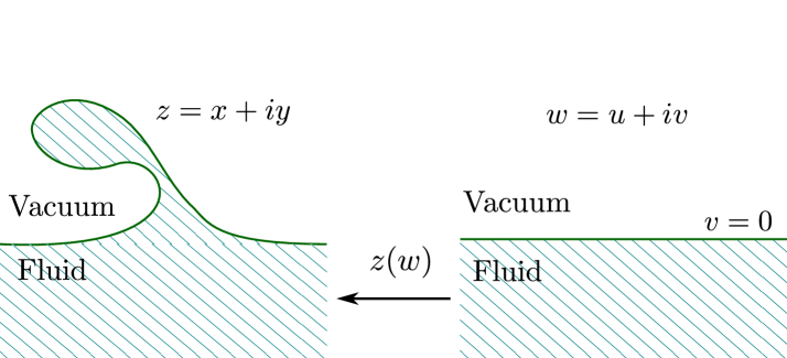
Figure 1: Shaded area represents the domain occupied by fluid in the physical plane $z=x+\mathrm{i}y$ (left) and the same domain in $w=u+\mathrm{i}v$ plane (right). Thick solid lines correspond to the fluid’s free surface.

We consider two-dimensional potential motion of ideal incompressible fluid with free surface of infinite depth. Fluid occupies the infinite region $-\infty<x<\infty$ in the horizontal direction $x$ and extends down to $y\to-\infty$ in the vertical direction $y$ as schematically shown on the left panel of Fig. 1. We assume that fluid is unperturbed both at $x\to\pm\infty$ and $y\to-\infty$.

We use a time-dependent conformal mapping

$$z(w,t)=x(w,t)+\mathrm{i}y(w,t)$$ (1)

of the lower complex half-plane $\mathbb{C}^{-}$ of the auxiliary complex variable $w\equiv u+\mathrm{i}v,\quad-\infty<u<\infty,$ into the area in $(x,y)$ plane occupied by the fluid. Here the real line $v=0$ is mapped into the fluid free surface (see Fig. 1) and $\mathbb{C}^{-}$ is defined by the condition $-\infty<v\leq 0$. Then the time-dependent fluid free surface is represented in the parametric form as

$$x=x(u,t),\ y=y(u,t).$$ (2)

A decay of perturbation of fluid beyond flat surface at $x(u,t)\to\pm\infty$ and/or $y\to-\infty$ requires that

$$z(w,t)\to w\ \text{for}\ |w|\to\infty,\ w\in\mathbb{C}^{-}.$$ (3)

The conformal mapping (1) imply that $z(w,t)$ is the analytic function of $w\in\mathbb{C^{-}}$ and

$$z_{w}\neq 0\ \text{for any}\ w\in\mathbb{C^{-}}.$$ (4)

Potential motion means that a velocity ${\bf v}$ of fluid is determined by a velocity potential $\Phi({\bf r},t)$ as ${\bf v}=\nabla\Phi$ with $\nabla\equiv(\frac{\p}{\p x},\frac{\p}{\p y})$. The incompressibility condition $\nabla\cdot{\bf v}=0$ implies the Laplace equation

$$\nabla^{2}\Phi=0$$ (5)

inside fluid, i.e. $\Phi$ is the harmonic function inside fluid. Eq. (5) is supplemented with a decaying boundary condition (BC) at infinity,

$$\nabla\Phi\to 0\ \text{for }\ |x|\to\infty\ \text{or}\ y\to-\infty.$$ (6)

The harmonic conjugate of $\Phi$ is a stream function $\Theta$ defined by

$$\Theta_{x}=-\Phi_{y}\ \text{and}\ \Theta_{y}=\Phi_{x}.$$ (7)

Similar to Eq. (6), we set without loss of generality a zero Dirichlet BC for $\Theta$ as

$$\Theta\to 0\ \text{}\ \text{for }\ |x|\to\infty\ \text{or}\ y\to-\infty.$$ (8)

We define a complex velocity potential $\Pi(z,t)$ as

$$\Pi=\Phi+\mathrm{i}\Theta.$$ (9)

is the complex coordinate. Then Eqs. (7) turn into Cauchy-Riemann equations ensuring the analyticity of $\Pi(z,t)$ in the domain of $z$ plane occupied by the fluid. A physical velocity with the components $v_{x}$ and $v_{y}$ (in $x$ and $y$ directions, respectively) is obtained from $\Pi$ as $\frac{d\Pi}{dz}=v_{x}-\mathrm{i}v_{y}$. The conformal mapping (1) ensures that the function $\Pi(z,t)$  (9) transforms into $\Pi(w,t)$ which is analytic function of $w$ for $w\in\mathbb{C^{-}}$ (in the bulk of fluid). Here and below we abuse the notation and use the same symbols for functions of either $w$ or $z$ (in other words, we assume that e.g. $\tilde{\Pi}(w,t)=\Pi(z(w,t),t)$ and remove $\tilde{~}{}$ sign). The conformal transformation (1) also ensures Cauchy-Riemann equations $\Theta_{u}=-\Phi_{v},\quad\Theta_{v}=\Phi_{u}$ in $w$ plane.

BCs at the free surface are time-dependent and consist of kinematic and dynamic BCs. A kinematic BC ensures that free surface moves with the normal velocity component $v_{n}$ of fluid particles at the free surface. Motion of the free surface is determined by a time derivative of the parameterization (2) while the kinematic BC is given by a projection into the normal direction as

$${\bf n}\cdot\left(x_{t},y_{t}\right)=v_{n}\equiv{\bf n}\cdot\nabla\Phi|_{x=x(u,t),\ y=y(u,t)},$$ (10)

where ${\bf n}=\frac{(-y_{u},x_{u})}{(x_{u}^{2}+y_{u}^{2})^{1/2}}$is the outward unit normal vector to the free surface and subscripts here and below means partial derivatives, $x_{t}\equiv\frac{\p x(u,t)}{\p t}$ etc.

Eq. (10) results in a compact expression

$$y_{t}x_{u}-x_{t}y_{u}=-\hat{H}\psi_{u}$$ (11)

for the kinematic BC as was found in Ref. Dyachenko et al. (1996), see also Ref. Dyachenko et al. (2019) for more details. Here

$$\psi(u,t)\equiv\Phi(u,v,t)|_{v=0}$$ (12)

is the Dirichlet BC for $\Phi$ at the free surface and

$$\hat{H}f(u)=\frac{1}{}\text{p.v.}\int^{+\infty}_{-\infty}\frac{f(u^{\prime})}{u^{\prime}-u}\mbox{d}u^{\prime}$$ (13)

is the Hilbert transform with p.v. meaning a Cauchy principal value of the integral. Real and imaginary parts of both $z$ and $\Pi$ at $v=0$ are related through $\hat{H}$ as follows

$$\tilde{x}\equiv x-u=-\hat{H}y,\quad\hat{H}x=y$$ (14)

and

$$\Theta|_{w=u}=\hat{H}\psi,\quad\psi=-\hat{H}\Theta|_{w=u},$$ (15)

see e.g. Appendix A of Ref. Dyachenko et al. (2019). Thus it is sufficient to find $y(u,t)$ and $\psi(u,t)$ while $x(u,t)$ and $\Theta(u,t)$ can be recovered from Eqs. (14) and (15).

A dynamic BC is given by the time-dependent Bernoulli equation (see e.g. Landau & Lifshitz (1989)) at the free surface,

$$\left.\left(\Phi_{t}+\dfrac{1}{2}\left(\nabla\Phi\right)^{2}+gy\right)\right|_{x=x(u,t),\ y=y(u,t)}=-P_{\alpha},$$ (16)

where $g$ is the acceleration due to gravity and $P_{\alpha}=-\frac{\alpha(x_{u}y_{uu}-x_{uu}y_{u})}{(x_{u}^{2}+y_{u})^{3/2}}$ is the pressure jump at the free surface due to the surface tension coefficient $\alpha$. Here without loss of generality we assumed that pressure is zero above the free surface (i.e. in vacuum). All results below apply both to surface gravity wave case ($g>0$) and Rayleigh-Taylor problem $(g<0)$. We also consider a particular case $g=0$ when inertia forces well exceed gravity force.

Eq. (16) can be transformed into

$$\psi_{t}y_{u}-\psi_{u}y_{t}+gyy_{u}=-\hat{H}\left(\psi_{t}x_{u}-\psi_{u}x_{t}+gyx_{u}\right)-\alpha\frac{\p}{\p u}\frac{x_{u}}{|z_{u}|}+\alpha\hat{H}\frac{\p}{\p u}\frac{y_{u}}{|z_{u}|},$$ (17)

thus representing the dynamic BC in the conformal variables, see Refs. Dyachenko et al. (2019) for details of such transformation.

Eqs. (11),(14) and (17) form a closed set of equations which is equivalent to Euler equations for dynamics of ideal fluid with free surface. The idea of using time-dependent conformal transformation like (1) to address systems equivalent/similar to Eqs. (11),(14) and (17) was exploited by several authors including Ovsyannikov (1973); Meison et al. (1981); Tanveer (1991, 1993); Dyachenko et al. (1996); Chalikov & Sheinin (1998, 2005); Chalikov (2016); Zakharov et al. (2002). We follow the analysis of Refs. Zakharov & Dyachenko (2012); Dyachenko et al. (2019) which found that Eqs. (11),(14) and (17) can be explicitly solved for the time derivatives $y_{t},\psi_{t}$ and rewritten in the non-canonical Hamiltonian form

$${\bf Q}_{t}=\hat{R}\frac{\delta H}{\delta{\bf Q}},\quad{\bf Q}\equiv\begin{pmatrix}y\\ \psi\end{pmatrix}$$ (18)

for the Hamiltonian variables $y(u,t)$ and $\psi(u,t),$ where$\hat{R}=\hat{\Omega}^{-1}=\begin{pmatrix}0&\hat{R}_{12}\\ \hat{R}_{21}&\hat{R}_{22}\end{pmatrix}$is $2\times 2$ skew-symmetric matrix operator with the components

$$\begin{split}&\hat{R}_{11}q=0,\ \hat{R}_{12}q=\frac{x_{u}}{J}q-y_{u}\hat{H}\left(\frac{q}{J}\right),\\ &\hat{R}_{21}q=-\frac{x_{u}}{J}q-\frac{1}{J}\hat{H}\left(y_{u}q\right),\quad\hat{R}_{21}^{\dagger}=-\hat{R}_{12},\\ &\hat{R}_{22}q=-\psi_{u}\hat{H}\left(\frac{q}{J}\right)-\frac{1}{J}\hat{H}\left(\psi_{u}q\right),\quad\hat{R}_{11}^{\dagger}=-\hat{R}_{11}.\end{split}$$ (19)

We call $\hat{R}=\hat{\Omega}^{-1}$ by the “implectic” operator (sometimes such type of inverse of the symplectic operator is also called by the co-symplectic operator, see e.g. Ref. Weinstein (1983)). Here the Hamiltonian $H$ is the total energy of fluid (kinetic plus potential energy in the gravitational field and surface tension energy) which is written in terms of the Hamiltonian variables as

$$H=-\frac{1}{2}\int\limits^{\infty}_{-\infty}\psi\hat{H}\psi_{u}\mbox{d}u+\frac{g}{2}\int\limits_{-\infty}^{\infty}y^{2}\,(1-\hat{H}y_{u})\mbox{d}u+\alpha\int\limits^{\infty}_{-\infty}\left(\sqrt{(1-\hat{H}y_{u})^{2}+y_{u}^{2}}-1+\hat{H}y_{u}\right)\mbox{d}u.$$ (20)

Eqs. (18) allows to define the Poisson bracket (see Ref. Dyachenko et al. (2019))

$$\begin{split}&\{F,G\}=\int\limits^{\infty}_{-\infty}\mbox{d}u\left(\frac{\delta F}{\delta y}\hat{R}_{12}\frac{\delta G}{\delta\psi}+\frac{\delta F}{\delta\psi}\hat{R}_{21}\frac{\delta G}{\delta y}+\frac{\delta F}{\delta\psi}\hat{R}_{22}\frac{\delta G}{\delta\psi}\right)\end{split}$$ (21)

which allows to rewrite Eq. (18) in terms of Poisson mechanics as

$$\begin{split}{\bf Q}_{t}=\{{\bf Q},H\}.\end{split}$$ (22)

Thus a functional $F$ is the constant of motion of Eq. (22) provided $\{{F},H\}=0.$

The Hamiltonian system (18)-(22) is the generalization of the results of Ref. Zakharov (1968). It was conjectured in Ref. Dyachenko & Zakharov (1994) that the system (14), (11) and (17) is completely integrable at least for the case of the zero surface tension. Since then the arguments pro and contra were presented, see e.g. Ref. Dyachenko et al. (2013a). Thus this question is still open.

The system (11),(14) and (17) has an infinite number of degrees of freedom. The most important feature of integrable systems is the existence of “additional” constants of motion which are different from “natural” motion constants (integrals) (see Refs. Arnold (1989); Zakharov & Faddeev (1971); Novikov et al. (1984)). For the system (11) , (14) and (17), the natural integrals are the energy $H$ (20), the total mass of fluid, and the horizontal component of the momentum. For $g=0,$ the vertical component of momentum is also the integral of motion. See Ref. Dyachenko et al. (2019) for the explicit expressions for these natural integrals.

In this paper we show that the system (11),(14) and (17) has a number of additional constants of motion. We cannot so far determine/estimate a total number of these constants. Instead we show examples of initial data such that the system has almost obvious, very simply constructed additional constants. We must stress that the number of known additional constants depends so far on the choice of initial data and can be made arbitrary large for the specific choices of initial data. Some of these new integrals of motion are functionals $y$ only. It follows from Eq. (21) that any functionals $F$ and $G,$ which depend only on $y$, commute with each other, i.e. $\{{F},G\}=0.$ We suggest that the existence of such commuting integrals of motion might be a sign of the Hamiltonian integrability of the free surface hydrodynamics. Such conjecture is in agreement with the history of the discovery of the Hamiltonian integrability of Korteweg de Vries equation, nonlinear Schrödinger and many other partial differential equations, see Refs. Gardner et al. (1967); Zakharov & Shabat (1972); Arnold (1989); Zakharov & Faddeev (1971); Novikov et al. (1984)).

Plan of the paper is the following. In Section 2 we introduce dynamic equations in the complex form for another unknowns $R$ and $V$ and consider an analytical continuation of solution into the upper complex half plane. Section 3 discusses non-persistence of pole solutions in both $R$ and $V$ variables within arbitrary small time while addressing that power law branch points are persistent. New constants of motion for gravity case but with zero surface tension are found in Section 4 for solutions of full hydrodynamic equations with simple complex poles in the original variables $z_{w}$ and $\Pi_{w}$. Section 5 provides another view of the new motion constants. Section 6 identifies new constants of motion to nonzero surface tension and second order poles. Section 7 discusses a global analysis for analytical continuation into multi-sheet Riemann surfaces and introduce a Kelvin theorem for phantom hydrodynamics. Section 8 provides a brief description of our numerical methods for simulation of free surface dynamics by spectrally accurate adaptive mesh refinement approach and a procedure for recovering of the structure of the complex singularities above fluid’s surface. Section 9 is devoted to the numerical results on free surface hydrodynamics simulations which provides a detailed verification of results of all other sections. Section 10 gives a summary of obtained results and discussion of future directions.

2 Dynamic equations in the complex form and analytical continuation of solution into the upper complex half plane

Dynamical Eqs. (11),(14) and (17) are defined on the real line $w=u$ with the analyticity of $z(w,t)$ and $\Pi(w,t)$ in $w\in\mathbb{C}^{-}$ taken into account through the Hilbert operator $\hat{H}.$ In this paper we consider also analytical continuation of these functions into the upper complex half plane $w\in\mathbb{C}^{+}.$ Both $z(w,t)$ and $\Pi(w,t)$ has time dependent complex singularities for $w\in\mathbb{C}^{+}$.

Using the Hilbert operator $\hat{H}$ (13), we introduce the operators

$$\hat{P}^{-}=\frac{1}{2}(1+\mathrm{i}\hat{H})\quad\text{and}\quad\hat{P}^{+}=\frac{1}{2}(1-\mathrm{i}\hat{H})$$ (23)

which are the projector operators of a function $q(u)$ defined at the real line $w=u$ into functions $q^{+}(u)$ and $q^{-}(u)$ analytic in $w\in\mathbb{C}^{-}$ and $w\in\mathbb{C}^{+}$, respectively, such that

$$q=q^{+}+q^{-}.$$ (24)

Here we assume that $q(u)\to 0$ for $u\to\pm\infty$. Eqs. (23) imply that

$$\hat{P}^{+}(q^{+}+q^{-})=q^{+}\quad\text{and}\quad\hat{P}^{-}(q^{+}+q^{-})=q^{-},$$ (25)

see more discussion of the operators (23) in Ref. Dyachenko et al. (2019).

Using Eqs. (9), (14), (15) and (23) we obtain that

$$\Pi=\psi+\mathrm{i}\hat{H}\psi=2\hat{P}^{-}\psi$$ (26)

and

$$z-u=-\hat{H}y+\mathrm{i}y=2\mathrm{i}\hat{P}^{-}y.$$ (27)

Analytical continuation of Eqs. (26) and (27) into the complex plane $w\in\mathbb{C}$ amounts to straightforward replacing $u$ by $w$ in the integral representation of $\hat{P}^{+}q(w)$ and $\hat{P}^{-}q(w)$ as detailed in Ref. Dyachenko et al. (2019).

Applying the projector $\hat{P}^{-}$ and using Eqs. (26), (27), one can rewrite (see Ref. Dyachenko et al. (2019)) the dynamical Eqs. (18), (19) in the complex form

$$z_{t}=\mathrm{i}Uz_{u},$$ (28)

$$\Pi_{t}=\mathrm{i}U\Pi_{u}-B-\mathcal{P,}$$ (29)

where

$$U\equiv\hat{P}^{-}(R\bar{V}+\bar{R}V)$$ (30)

is the complex transport velocity with

$$\mathcal{P}=-\mathrm{i}g(z-w)-2\mathrm{i}\alpha\hat{P}^{-}(Q_{u}\bar{Q}-Q\bar{Q}_{u}),$$ (31)

$$Q\equiv\frac{1}{\sqrt{z_{u}}}=\sqrt{R}$$ (32)

and

$$B\equiv\hat{P}^{-}(|V|^{2}).$$ (33)

A complex conjugation $\bar{f}(w)$ of $f(w)$ in Eqs. (30), (31), (33) and throughout this paper is understood as applied with the assumption that $f(w)$ is the complex-valued function of the real argument $w$ even if $w$ takes the complex values so that

$$\bar{f}(w)\equiv\overline{f(\bar{w})}.$$ (34)

That definition ensures the analytical continuation of $f(w)$ from the real axis $w=u$ into the complex plane of $w\in\mathbb{C.}$

Another equivalent complex form of the dynamical Eqs. (18), (19) are the “Dyachenko” equations (Dyachenko (2001))

$$\frac{\partial R}{\partial t} =\mathrm{i}\left(UR_{u}-RU_{u}\right),$$ (35)

$$\frac{\partial V}{\partial t} =\mathrm{i}\left[UV_{u}-RB_{u}\right]+g(R-1)-2\alpha R\hat{P}^{-}\frac{\p}{\p u}(Q_{u}\bar{Q}-Q\bar{Q}_{u}),$$ (36)

where

$$R=\frac{1}{z_{u}},$$ (37)

$$V=\mathrm{i}\frac{\p\Pi}{\p z}=\mathrm{i}R\Pi_{u}$$ (38)

are the new unknowns first introduced in Ref. Dyachenko (2001). Eqs. (35) and (36) can be obtained by differentiating Eqs. (28), (29) over $u$ and using the definitions (37) and (38), see also Ref. Dyachenko et al. (2019) for more details.

3 Local analysis: non-persistence of poles in $R$ and $V$ variables and persistence of power law branch points

All four functions $R$, $V$, $U$ and $B$ of Eqs. (30), (33), (35) and (36) must have singularities in the upper half-plane $w\in\mathbb{C}^{+}$ while being analytic for $w\in\mathbb{C}^{-}$. At the initial time $t=0,$ any singularity for $w\in\mathbb{C}^{+}$ are allowed including poles, branch points, etc. We are interested in singularities that keep their nature in the course of evolution to at least a finite duration of time. This “persistence” requirement is very restrictive. It would be extremely attractive to find solutions containing only pole-type singularities such that $R$, $V$, $U$ and $B$ would be the rational functions of $w$. There are examples of different reductions/models of free surface hydrodynamics which allows such rational solutions. They include a free surface dynamics for the quantum Kelvin-Helmholtz instability between two components of superfluid Helium (Lushnikov & Zubarev, 2018); an interface dynamic between ideal fluid and light highly viscous fluid Lushnikov (2004), and a motion of the dielectric fluid with a charged and ideally conducting free surface in the vertical electric field (Zubarev, 2000, 2002, 2008).

However, for Dyachenko Eqs. (30),(33), (35) and (36) without surface tension, which takes the following form

$$\frac{\partial R}{\partial t} =\mathrm{i}\left(UR_{u}-RU_{u}\right),$$ (39)

$$\qquad U =\hat{P}^{-}(R\bar{V}+\bar{R}V),\quad B=\hat{P}^{-}(|V|^{2}),$$ (40)

$$\frac{\partial V}{\partial t} =\mathrm{i}\left[UV_{u}-RB_{u}\right]+g(R-1),$$ (41)

rational solutions are not known and we conjecture that they cannot be constructed to satisfy $R(w)\neq 0$ and $|R(w)|<\infty$ for all $w\in\mathbb{C}^{-}$ (as required by the conformal mapping (1) with the condition (4)). The only known exception is the trivial case

$$g=0,\quad\frac{\partial R}{\partial t}\equiv 0,\quad\text{and}\quad V\equiv 0,$$ (42)

i.e. a stationary solution of fluid at rest without gravity. In that case any singularities (including rational solutions) are allowed in $R(w)$ for $w\in\mathbb{C}^{+}$ and these singularities remain constant in time. We notice that in Eqs. (39)-(41) and throughout this paper we use the partial derivatives over $w$ and $u$ interchangeably by assuming the analyticity in $w.$

In this section we provide the local analysis on existence vs. nonexistence of persistent poles singularities in Eqs. (39)-(41). The analysis is local because we use the Laurent series of solutions of free surface hydrodynamics at any moving point $w=a(t)$, $Im(a)>0$. It means that we are not restricted to rational solutions because such local analysis does not exclude the existence of branch points for $w\neq a(t),\ w\in\mathbb{C}^{+}$. In the next section we also provide the local analysis on the persistence of power law branch points.

We note that the conformal map (1) and the definition (37) imply that $R(w)\neq 0$ for $w\in\mathbb{C}^{-}$ and, respectively,

$$\bar{R}(w)\neq 0\ \text{for}\ w\in\mathbb{C}^{+}.$$ (43)

We stress that this is a fact of essential importance. Here and below we often omit the second argument $t$ when we focus on analytical properties in $w$.

Theorem 1: Eqs. (39)-(41) have no persistent in time solution, such that both $R$ and $V$ have only simple poles singularities at a moving point $w=a(t),$ and a residue $V_{-1}$ of $V$ is not identically zero in time.

We prove Theorem 1 “ad absurdum”. Simple poles imply that $V(w)$ and $R(w)$ at $w=a\in\mathbb{C}^{+}$ can be written as

$$V=\frac{V_{-1}}{w-a}+V_{reg},\quad$$ (44)

$$R=\frac{R_{-1}}{w-a}+R_{reg},\quad$$ (45)

where

$$V_{reg}=\sum\limits_{j=0}^{\infty}{V_{j}}{(w-a)^{j}}$$ (46)

and

$$R_{reg}=\sum\limits_{j=0}^{\infty}{R_{j}}{(w-a)^{j}}$$ (47)

are the regular parts of $V$ and $R$ (these regular parts are the analytic function at $w=a$). The coefficients $R_{j},\ V_{j},\ j=-1,0,\ldots$ and $a$ in Eqs. (44)-(47) are assumed to be the functions of $t$ only. In a similar way, below we designate by the subscript $``reg"$ the nonsingular part of the all functions at $w=a.$ The functions $U(w)$ and $B(w)$ (40) generally also have simple poles at $w=a$, so that we write them as

$$U=\frac{U_{-1}}{w-a}+U_{reg},\quad U_{reg}=\sum\limits_{j=0}^{\infty}{U_{j}}{(w-a)^{j}},$$ (48)

$$B=\frac{B_{-1}}{w-a}+B_{reg},\quad B_{reg}=\sum\limits_{j=0}^{\infty}{B_{j}}{(w-a)^{j}}.$$ (49)

To understand validity of these equations and find $U_{-1}$ and $B_{-1}$ we notice that using Eqs. (23)-(25) we can rewrite the definitions (40) as

$$\begin{split}&U=R\bar{V}+\bar{R}V-\hat{P}^{+}(R\bar{V}+\bar{R}V),\\ &B=V\bar{V}-\hat{P}^{+}(V\bar{V}).\end{split}$$ (50)

The functions $\hat{P}^{+}(R\bar{V}+\bar{R}V)$ and $\hat{P}^{+}(V\bar{V})$ are analytic at $w=a\in\mathbb{C}^{+}$ thus they only contribute to $U_{reg}$ and $B_{reg},$ respectively. The functions $\bar{R}$ and $\bar{V}$ are also analytic at $w=a$ with Taylor series representations

$$\bar{R}(w)\equiv R_{c}+\sum\limits_{j=1}^{\infty}{R_{c,j}}{(w-a)^{j}}.$$ (51)

and

$$\bar{V}(w)\equiv V_{c}+\sum\limits_{j=1}^{\infty}{V_{c,j}}{(w-a)^{j}},$$ (52)

where $R_{c}\equiv\bar{R}(a)$ and $V_{c}\equiv\bar{V}(a)$ are zero order terms and ${R_{c,j}}$, ${V_{c,j}}$ are the coefficients of the higher order terms of the respective power series.

Eqs. (50)-(52) imply that generally $U$ and $B$ have the same types of singularities as $R$ and $V$ except special cases when poles of either $R$ or $V$ are canceled out. Calculating residues of $R\bar{V}+\bar{R}V$ and $|V|^{2}$ at $w=a$ we obtain that

$$\begin{split}&U_{-1}=R_{c}V_{-1}+V_{c}R_{-1},\\ &B_{-1}=V_{c}V_{-1,}\\ &R_{c}\equiv\bar{R}(a)\neq 0,\quad V_{c}\equiv\bar{V}(a),\end{split}$$ (53)

where we used Eqs. (44)-(49), (51) and (52). Also $R_{c}=\bar{R}(a)\neq 0$ follows from the general condition (43).

According to Theorem 1’s assumption, $V_{-1}\neq 0$. Calculating the partial derivative of Eq. (44),

$$\frac{\partial V}{\partial t} =\frac{a_{t}V_{-1}}{(w-a)^{2}}+\frac{(V_{-1})_{t}}{w-a}+(V_{reg})_{t},$$ (54)

we see that the left-hand side (l.h.s.) of Eq. (41) has at most (if $a_{t}\neq 0$) the second order pole. At the same time, the right-hand side (r.h.s.) of Eq. (41) has the third order pole $\frac{-\mathrm{i}R_{c}V_{-1}^{2}}{(w-a)^{3}}$ because $R_{c}\neq 0,$ where we used Eqs. (53). It implies that $V_{-1}=0$ is required to match l.h.s and r.h.s. of Eq. (41) which contradicts the initial assumption thus completing the proof of Theorem 1.

Consider now a more difficult case $R_{-1}\neq 0$ and $V_{-1}=0.$ Then Eqs. (44)-(49) and (49)-(53) imply that $V(w)$ and $B(w)$ are the regular functions at $w=a.$ If $V_{c}\neq 0$ then $U(w)$ has a pole according to Eqs. (48) and (53). It leads to the formation of second order pole in Eq. (39) which is canceled out provided

$$a_{t}=\mathrm{i}\left[R_{0}V_{c}-U_{0}\right],$$ (55)

where $U_{0}$ cannot be obtained from the local analysis of this section because it requires to evaluate the projector in Eq. (50) which needs a global information about $V$ and $R$ in the complex plane $w\in\mathbb{C}.$

At the next order, $(w-a)^{-1}$, we obtain that

$$(R_{-1})_{t}=-2\mathrm{i}R_{-1}(U_{1}-R_{1}V_{c})$$ (56)

and

$$B_{1}={-\mathrm{i}g}{}+V_{1}V_{c},$$ (57)

where again $U_{1}$ and $B_{1}$ can be found only if $V$ and $R$ are known globally in the complex plane $w\in\mathbb{C}.$ The conditions (55)-(57) must be satisfied during evolution. Similar conditions can be obtained from terms of orders $(w-a)^{0},(w-a)^{1},\ldots$ to give equations for time derivatives of coefficients of the series of regular part of $R$ and $V$ (e.g. the order $(w-a)^{0}$ provides the explicit expressions for $(R_{0})_{t}$ and $(V_{0})_{t}$ etc).

We conclude that the local analysis does not exclude a possibility of the existence of the persistent in time solution with $R_{-1}\neq 0$ and $V_{-1}=0.$ The exceptional case, when the global information is not needed, is $V\equiv 0$ (it means that $U\equiv 0$ and $B\equiv 0$) which implies that Eq. (57) cannot be satisfied for $g\neq 0.$ Then by contradiction we conclude that

$$R_{-1}=0,\ \text{for}\ V\equiv 0\ \text{and}\ g\neq 0,$$ (58)

i.e. no persistent poles exist in that case even for the pole only in $R$ with $V$ analytic at that point.

Theorem 1 can be generalized to prove nonpersistence of the same higher order poles $R$ with $V.$ The analysis of that case is beyond the scope of this paper.

We note that the analysis of Ref. Tanveer (1993) assumed that both $\Pi_{u}$ and $z_{u}$ are analytic in the entire complex plane $w\in\mathbb{C}$ at $t=0$ (Ref. Tanveer (1993) actually considered periodic solutions with an additional symmetry in horizontal direction with the fluid domain mapped to the unit ball, but we can adjust results of that Ref. to our conformal map). In terms of $R$ and $V,$ it means that poles are possible only if $z_{u}$ has a regular $n$th order zero at $w=a$ with $n=1,2,\ldots$. Ref. Tanveer (1993) assumed $z_{u}(w=a,t=0)=0$ and $z_{uu}(w=a,t=0)\neq 0$, i.e. $n=1.$ Two cases were considered in Ref. Tanveer (1993) for $a\in\mathbb{C}^{+}$: (a) $\Pi_{u}(w=a,t)\neq 0$ and (b) $\Pi_{u}(w,t)\equiv 0$ in $\mathbb{C}$. The case (a) implies that $V_{-1}(w=a,t=0)\neq 0$ and $R_{-1}(w=a,t=0)\neq 0.$ Then our Theorem 1 above proves that such initial condition cannot lead to persistent pole solutions. It agrees with the asymptotic result of Ref. Tanveer (1993) that a couple of branch points are formed from that initial conditions during an infinite small duration of time. The case (b) of Ref. Tanveer (1993) means that $V\equiv 0$ for $t=0$ which has no poles as proven in Eq. (58). Refs. Kuznetsov et al. (1993, 1994) considered a related case $R\equiv 1$ and a pole in $V$ at $t=0$ which results in the formation of a couple of branch points in an infinite small duration of time. That result is again consistent with Theorem 1. Thus our results on the non-existence of persistent poles are in full agreement with the particular conditions of Refs. Tanveer (1993); Kuznetsov et al. (1993, 1994).

We also note that taking into account a nonzero surface tension, i.e. working with Eqs. (30),(33), (35) and (36) instead of Eqs. (39)-(41), immediately shows that pole singularity both for $R$ and $V$ is non-persistent because the dependence of surface tension terms of $Q=\sqrt{R}$ introduces the square root singularity into Eq. (36) which cannot be compensated by other terms with poles.

Contrary to poles analyzed above, power law branch points are persistent in time for free surface dynamics which can be shown by the local analysis qualitatively similar to the pole analysis above. The detailed analysis of the persistence of power branch points is however beyond the scope of this paper. The most common type of branch points, observed in our numerical experiments is $\gamma=\frac{1}{2}$ which is consistent with the results of Refs. Grant (1973); Tanveer (1991, 1993); Kuznetsov et al. (1993, 1994). Square root singularities have been also intensively studied based on the representation of vortex sheet in Ref. Moore (1979); Meiron et al. (1982); Baker et al. (1982); Krasny (1986); Caflisch & Orellana (1989); Caflisch et al. (1990); Baker & Shelley (1990); Shelley (1992); Caflisch et al. (1993); Baker et al. (1993); Cowley et al. (1999); Baker & Xie (2011); Zubarev & Kuznetsov (2014); Karabut & Zhuravleva (2014); Zubarev & Karabut (2018).

Particular solution of Eqs. (39)-(41) is Stokes wave which is a nonlinear periodic gravity wave propagating with the constant velocity  (Stokes, 1847, 1880). In the generic situation, when the singularity of Stokes wave is away from the real axis (non-limiting Stokes wave), the only allowed singularity in $\mathbb{C}$ is $\gamma=1/2$ as was proven in Ref. Tanveer (1991) for the first (physical) sheet of the Riemann surface and in Ref. Lushnikov (2016) for the infinite number of other (non-physical) sheets of Riemann surface. Refs. Dyachenko et al. (2013b, 2016); Lushnikov et al. (2017) provided detailed numerical verification of these singularities. The limiting Stokes wave is the special case $\gamma=1/3$ with $a=\mathrm{i}Im(a)$. Also Ref. Tanveer (1993) suggested the possibility in exceptional cases of the existence of $\gamma=1/n$ singularities with $n$ being any positive integer as well as singularities involving logarithms.

4 New constants of motion for gravity case but with zero surface tension

Assume that both functions $R$ and $V$ are analytic on a Riemann surface $\Gamma$. The complex plane of $w$ is the first sheet of this surface, which we assume to contain a finite number of branch points $w=w_{m},\ m=1,2,\ldots,M$.

We now address the question if $R$ could have isolated zeros at some other points of $\mathbb{C}^{+}.$ (We remind that $R(w)\neq 0$ for $w\in\mathbb{C}^{-}$ because the mapping (1) is conformal.) Assume that $R$ has a simple zero at $w=a(t)$, i.e. $R(a)=0$ and $R_{u}(a)\neq 0$. We assume that the functions $R$ and $V$ are analytic at that point witch implies through Eqs. (50) that the functions $U$ and $B$ (40) are also analytic at that point with the Taylor series

$$R=\qquad\,{R_{1}}{(w-a)}+{R_{2}}{(w-a)^{2}}+\ldots,\ R_{1}\neq 0,$$ (59)

$$V={V_{0}+V_{1}}{(w-a)}+{V_{2}}{(w-a)^{2}}+\ldots,$$ (60)

as well as we use the Taylor series

$$U={U_{0}+U_{1}}{(w-a)}+{U_{2}}{(w-a)^{2}}+\ldots,$$ (61)

$$B={B_{0}+B_{1}}{(w-a)}+{B_{2}}{(w-a)^{2}}+\ldots.$$ (62)

Similar to Section 3, by plugging in Eqs. (59)-(62) into Eqs. (39) and (41) and collecting terms of the same order of $(w-a)^{j}$ we obtain for $j=0$ that

$$a_{t}=-\mathrm{i}U_{0}$$ (63)

and

$$(V_{0})_{t}=-g.$$ (64)

The order $j=1$ results in

$$(R_{1})_{t}=0$$ (65)

and

$$(V_{1})_{t}=gR_{1}+\mathrm{i}(U_{1}V_{1}-B_{1}R_{1}).$$ (66)

Equations (64) and (65) are of fundamental importance. Eq. (65) states that both in absence and in presence gravity

$$R_{1}=\mbox{const}\equiv\frac{1}{c_{1}^{(1)}},$$ (67)

where $c_{1}^{(1)}$ is the complex time-independent constant. Eq.  (68) results in the trivial dependence on time,

$$V_{0}(t)=-gt+e_{1}^{(1)},$$ (68)

where $e_{1}^{(1)}$ is the complex constant defined by the initial condition, $e_{1}^{(1)}=V_{0}(t=0).$ Here the subscript $``1"$ stands for the first order of zeros of $R$ in Eq. (59). We conclude that each simple zero of function $R$ generates four additional real integrals of motion. Two of them are the real and imaginary parts of $c_{1}^{(1)}=1/R_{1}.$ Two others are the real and imaginary parts of $e_{1}^{(1)}=V_{0}(t)+gt.$ In addition, $V_{0}(t)$ is either obeys the trivial linear dependence on time for nonzero gravity $g\neq 0$ or coincide with $e_{1}^{(1)}$ for $g=0.$ Eq. (63) provides another important relation showing that $-\mathrm{i}U_{0}$ is “the transport velocity” which governs the propagation of the zeros of the function $R$ in the complex plane of $w$.

Taking into account all $N$ isolated simple zeros of $R$ at $w=a^{(j)},\ j=1,\ldots,N$ and designating by the superscript $``(j)"$ the corresponding $j$th zero, we obtain from Eqs. (67) and (68) that $R_{1}^{(n)}=\mbox{const}\equiv 1/c_{1}^{(n)}$ and $V_{0}^{(n)}(t)=-gt+e_{1}^{(n)}$. Then we notice that any difference $e_{1}^{(j)}-e_{1}^{(n)},\ j,n=1,\ldots N,\ j\neq n,$ is the true integral of motion even for $g\neq 0.$

We conclude that $N$ simple isolated zeros of $R,$ separated from branch points, imply for $g\neq 0$ the existence of $4N-1$ independent new constants of motion $Re(c_{1}^{(n)}),$ $Im(c_{1}^{(n)}),n=1,\ldots,N$, $Re(e_{1}^{(n)}-e_{1}^{(N)}),$ $Im(e_{1}^{(n)}-e_{1}^{(N)}),\ n=1,\ldots,N-1$, and $Im(e_{1}^{(N)})$ as well as one linear function of time $Re(V_{0}^{(N)})=-gt+Re(e_{1}^{(N)})$. For zero gravity $g=0$ we have $4N$ independent new constants of motion $Re(c_{1}^{(n)}),$ $Im(c_{1}^{(n)}),Re(e_{1}^{(n)}),$ $Im(e_{1}^{(n)}),\ n=1,\ldots,N$.

Section 9 below demonstrates, in a number of particular cases, the independence of these motion constants on time in full nonlinear simulations of Eqs. (39)-(41).

Using definitions (37) and (38), we obtain from Eqs. (59) and (60) that

$$\begin{split}&z_{w}=\frac{1}{R_{1}(w-a)}+(z_{w})_{reg},\\ &\Pi_{w}=\frac{-\mathrm{i}V_{0}}{R_{1}(w-a)}+(\Pi_{w})_{reg}.\end{split}$$ (69)

Eq. (67), (68) and (69) imply that the residues (i.e. the coefficients of $(w-a)^{-1}$ of Laurent series),

$$\underset{w=a}{Res}(z_{w})=\frac{1}{R_{1}}=c_{1}^{(1)}=const$$ (70)

and $\underset{w=a}{Res}(\Pi_{w})=\frac{-\mathrm{i}V_{0}}{R_{1}}=-\mathrm{i}c_{1}^{(1)}e_{1}^{(1)}=const,$ of both $z_{w}$ and $\Pi_{w}$ are constants of motion for $g=0$. For $g\neq 0,$ $\underset{w=a}{Res}(z_{w})$ remains the integral of motion while

$$\underset{w=a}{Res}(\Pi_{w})=-\mathrm{i}c_{1}^{(1)}[-gt+e_{1}^{(n)}],$$ (71)

i.e. it has the linear dependence on time. Section 5 provides another way to straightforward derivation that these residues are constants of motion.

A Poisson bracket (21) between any motion constant is a motion constant itself (see e.g. Ref. Arnold (1989)). Together such motion constants form a Lie algebra. We conjecture that this Lie algebra is commutative. However, in this paper we are able to prove only a weaker statement that

$$\{c_{1}^{(n)},c_{1}^{(k)}\}=0$$ (72)

for any $n,k=1,\ldots,N.$ The proof is almost trivial and relies on the fact that all $c_{1}^{(n)}$ integrals are determined by the shape of the free surface $z(u,t)$, ie.e they are functionals of $z$ only. Hence

$$\frac{\delta c_{1}^{(n)}}{\delta\psi}=0,\ n=1,\ldots,N,$$ (73)

and Eq. (72) immediately follows from the Poisson bracket definition (21). The question about an explicit calculation of Poisson brackets $\{c_{1}^{(n)},e_{1}^{(k)}\}$ and $\{e_{1}^{(n)},e_{1}^{(k)}\},$ $n,k=1,\ldots,N,$ remains open.

We note that the existence of the arbitrary number of the integrals of motion was not addressed in Ref. Tanveer (1993) because it focused on the particular case of analytic analytic initial data in the entire complex plane $w\in\mathbb{C}.$

5 Another view of the new motion constants

In this section we use the dynamical Eqs. (28), (29) with $\alpha=0.$ It is useful to introduce new functions

$$\rho\equiv z_{u}=\frac{1}{R}\ \text{and}\ W\equiv\Pi_{u}=-\mathrm{i}\frac{V}{R}.$$ (74)

Then differentiating Eqs. (28) and (29) over $u$ together with the definitions (74) imply that

$$\begin{split}&\rho_{t}=\mathrm{i}(U\rho)_{u},\\ &W_{t}=\mathrm{i}(UW)_{u}-B_{u}+\mathrm{i}g(\rho-1).\end{split}$$ (75)

Let us address a question about possible singularities of the functions $\rho$ and $W$. We assume that the functions $R$ and $V$ (37), (38) have only a finite number of branch points for $w\in C^{+}.$ Apparently, $\rho$ and $W$ generally inherit these branch points (with the only exception of the possible cancellation of some branch points because $W=-\mathrm{i}V/R)$ but they cannot have any additional branch point. In other way, if a branch point appears in $\rho$ and $W$ at some moment of time, then it immediately implies a branch point creation in both $R$ and $V.$

However, $\rho$ and $W$ can have poles in the domains of the regularity of $R$ and $V.$ Indeed, assume that $R$ has a regular pole of order $m$ at $w=a$ while $V$ is regular and nonzero at $w=a$. It means that at $w=a$ both $R$ and $V$ can be represented by Taylor series

$$R=\qquad\qquad\qquad\qquad{R_{m}}{(w-a)^{m}}+\ldots,\ R_{m}\neq 0,$$ (76)

$$V={V_{0}+V_{1}}{(w-a)}+{V_{2}}{(w-a)^{2}}+\ldots.$$ (77)

Then Eqs. (74),(76) and (77) imply Laurent series

$$\begin{split}&\rho=\sum\limits^{\infty}_{j=-m}(w-a)^{j}\rho_{j},\\ &W=\sum\limits^{\infty}_{j=-m}(w-a)^{j}W_{j}.\end{split}$$ (78)

Here $\rho_{-1}$ and $W_{-1}$ are the residues or $\rho$ and $W$ at $w=a$ which can be represented by the contour integrals

$$\rho_{-1}=\frac{1}{2\pi\mathrm{i}}\oint\limits_{C}\rho\,\mbox{d}w=\frac{1}{2\pi\mathrm{i}}\oint\limits_{C}\frac{\mbox{d}w}{R}$$ (79)

and

$$W_{-1}=\frac{1}{2\pi\mathrm{i}}\oint\limits_{C}W\,\mbox{d}w=-\frac{1}{2\pi}\oint\limits_{C}\frac{V\,\mbox{d}w}{R},$$ (80)

where $C$ is the counterclockwise closed contour around $w=0$ which is taken small enough to avoid including any branch point in the interior.

A direct integration of Eqs. (75) over the contour $C$ implies together with Eqs. (79) and (80) that

$$\frac{d}{dt}\rho_{-1}=0,$$ (81)

$$\frac{d}{dt}W_{-1}=\mathrm{i}g\rho_{-1},$$ (82)

which is another way to recover the results of Section 4 (Eqs. (70) and (71)) in terms of $\rho$ and $W.$ In particular, Eq. (81) means that $\rho_{-1}$ is the constant of motion and $W_{-1}$ is the motion constant only for $g=0$ while generally

$$W_{-1}=W_{-1}^{(0)}+\mathrm{i}g\rho_{-1}t,$$ (83)

with $W_{-1}^{(0)}$ being the complex constant.

Thus poles in $\rho$ and $W$ are persistent in time (at least during a finite time while $w=a$ remains a regular point of both $\rho$ and $W$) which suggests the following decomposition

$$\begin{split}&\rho=\rho_{rational}+\rho_{b},\\ &W=W_{rational}+W_{b},\end{split}$$ (84)

where $\rho_{rational}$ and $W_{rational}$ are the rational functions of $w$ while $\rho_{b}$ and $W_{b}$ generally have branch points.

Assume that at the initial time $t=0$, both $\rho$ and $W$ are purely rational, i.e. $\rho_{b}|_{t=0}=W_{b}|_{t=0}\equiv 0.$ As a simple particular case one can assume that these rational functions have only simple poles with residues $\rho_{-1}^{(k)}$ and $W_{-1}^{(k)}$ at $N$ points $w=a_{k},\ Im(a_{k})>0,\ k=1,2,\ldots,N$ as follows

$$\rho|_{t=0}=1+\sum\limits^{N}_{k=1}\frac{\rho_{-1}^{(k)}}{w-a_{k}},\quad W|_{t=0}=\sum\limits^{N}_{k=1}\frac{W_{-1}^{(k)}}{w-a_{k}},$$ (85)

where 1 in r.h.s of the first equation ensures the correct limit (3). Generally these points might be different for $\rho$ and $W$ but our particular choice of the same points corresponds to the common poles originating from the zeros of $R$ in Eqs. (74). This type of initial conditions is studied numerically in Section 9. Note that the initial conditions (85) imply logarithmic singularities at $w=a_{k},\ k=1,2,\ldots,N$ in both $z$ and $\Pi$ through the definitions (74) provided $\rho_{-1}^{(k)}\neq 0$ and $W_{-1}^{(k)}\neq 0$.

Bringing Eqs. (85) to the common denominator, we immediately conclude that $\rho|_{t=0}$ has $N$ zeros (counting according to their algebraic multiplicity) at some points $w=b_{k},\ k=1,2,\ldots,N$. Eq. (4) requires that $Im(b_{k})>0$ for all $k=1,2,\ldots,N$ which must be taken into account in choosing initial conditions (85) for simulations.

In a general position $W|_{w=b_{k}}\neq 0.$ Assume that $w=b_{k}$ is $m$th order zero of $\rho|_{t=0}$. Then Eqs. (74) imply that the Laurent series of both $R$ and $V$ have poles of order $m.$ According to Section 3 such poles are not persistent in time meaning that in arbitrary small time they turn into branch points.

The branch point at $w=b_{k}$ is generally moving with time, i.e. $b_{k}=b_{k}(t).$ At the initial time $t=0$, the point $w=b_{k}$ is separated from all poles $w=a_{j},\ j=1,2,.\ldots,N$ in Eqs. (85). It means that at least during a finite time $w=b_{k}$ will remain separated from from poles $w=a_{j}(t),\ j=1,2,.\ldots,N$ which move according to Eq. (63) (this equation is also valid for arbitrary $m$ as shown in Section 6 below for $m=2$, Eq. (91)). During that finite time one can write a decomposition (84) as

$$\begin{split}&\rho=1+\sum\limits^{m}_{j=1}\sum\limits^{N}_{k=1}\frac{\rho_{-j}^{(k)}}{(w-a_{k}(t))^{j}}+\rho_{b},\\ &W=\sum\limits^{m}_{j=1}\sum\limits^{N}_{k=1}\frac{W_{-j}^{(k)}(t)}{(w-a_{k}(t))^{j}}+W_{b},\end{split}$$ (86)

where the “non-rational” terms $\rho_{b}$ and $W_{b}$ are identically zero at $t=0.$ Here $\rho_{-1}^{(k)}$ is the motion constant and $W_{-1}^{(k)}(t)$ is the linear function of time according to Eqs. (81) and (83). Results of the numerical experiment of Section 9 support that decomposition scenario completely.

6 New constants of motion for nonzero surface tension and second order poles in $z_{w}$ and $\Pi_{w}$

If taking into account the nonzero surface tension, $\alpha\neq 0,$ then instead of Eqs. (39)-(41) we have to consider more general Eqs. (30),(33), (35) and (36). Expressing $Q=\sqrt{R}$ through $R$ we obtain from Eq. (36) that

$$\frac{\partial V}{\partial t}=\mathrm{i}\left[UV_{u}-R\hat{P}^{-}\frac{\p}{\p u}(|V|^{2})\right]+g(R-1)-\alpha R\hat{P}^{-}\frac{\p}{\p u}\left(\frac{R_{u}\sqrt{\bar{R}}}{\sqrt{R}}-\frac{\bar{R}_{u}\sqrt{R}}{\sqrt{\bar{R}}}\right).$$ (87)

Assume that initially $R$ and $V$ satisfy Eqs. (59)-(60). Plugging them into r.h.s. of Eq. (87), one obtains at the leading power of $w-a$ that

$$\frac{\partial V}{\partial t}\propto\frac{1}{\sqrt{w-a}},$$ (88)

i.e. a square root singularity appears in $V$ in the infinitely small time. Thus the analysis of Section 4 fails for nonzero surface tension. However, we can now consider the double zero in $R$, i.e. Eq. (59) is replaced by

$$R=\qquad\qquad\qquad\qquad{R_{2}}{(w-a)^{2}}+\ldots,\ R_{2}\neq 0,$$ (89)

$$V={V_{0}+V_{1}}{(w-a)}+{V_{2}}{(w-a)^{2}}+\ldots,$$ (90)

and, respectively, the square root disappears in $\sqrt{R}$.

Plugging Eqs. (61), (62),(89) and (90) into Eqs. (39) and (87), and collecting terms of the same order of $(w-a)^{j}$ we obtain, similar to Section 4, at order $j=0$ that

$$a_{t}=-\mathrm{i}U_{0}$$ (91)

and

$$(V_{0})_{t}=-g,$$ (92)

which are exactly the same as Eqs. (63) and (64) and which implies that Eq. (68) is now trivially replaced by

$$V_{0}(t)=-gt+e_{2}^{(1)},$$ (93)

where $e_{2}^{(1)}$ is the constant defined by the initial condition, $e_{2}^{(1)}=V_{0}(t=0).$ Here the subscript $``2"$ stands for the second order of zero of $R$ in Eq. (89).

The orders $j=1$ and $j=2$ result in

$$(R_{2})_{t}=\mathrm{i}R_{2}U_{1}$$ (94)

and

$$(V_{1})_{t}=\mathrm{i}V_{1}U_{1},$$ (95)

where we do not show an explicit expression for $(V_{2})_{t}$ which appears not much useful.

Excluding $U_{1}$ from Eqs. (94) and (95) we obtain the constant of motion

$$\frac{V_{1}}{R_{2}}=\mbox{const}\equiv f_{2}^{(1)}.$$ (96)

We note that the surface tension coefficient $\alpha$ does not contribute to Eqs. (93) and (96) ($\alpha$ contributes only to the expression for $(V_{2})_{t}$ and higher orders in powers of $w-a)$. Thus Eq. (96) is valid for arbitrary $g$ and $\alpha$.

Eqs. (37),(38),(76) and (77) imply that Eq. (69) is replaced by Laurent series

$$\begin{split}&z_{w}=\frac{1}{R_{2}(w-a)^{2}}-\frac{R_{3}}{R_{2}^{2}(w-a)}+O\left((w-a)^{0}\right),\\ &\Pi_{w}=\frac{-\mathrm{i}V_{0}}{R_{2}(w-a)^{2}}+\frac{\mathrm{i}(R_{3}V_{0}-R_{2}V_{1})}{R_{2}^{2}(w-a)}+O\left((w-a)^{0}\right).\end{split}$$ (97)

However, Eqs. (92) and (96) do not exhaust all integrals of motion for the case of the second order pole of this section. For that we note that the results of Section 5 on time independence of $\rho_{-1}=\underset{w=a}{Res}(z_{w})$ and linear dependence of $W_{-1}=\underset{w=a}{Res}(\Pi_{w})$ on time (see Eqs. (81) and (82)) are true for the second order pole as well as they remain valid for $\alpha\neq 0$. We note that it is possible to derive Eqs. (81) and (82) by direct computations in $R$ and $V$ variables, similar to the derivation of Eq. (96), but we do not provide it here because the analysis of Section 5 is much more elegant for these residues. Thus Eq. (81) imply that it is natural to replace the definition of the motion constant $c_{1}^{(1)}$ from Eq. (70) of Section 4 for the first order pole by

$$\underset{w=a}{Res}(z_{w})\equiv c_{2}^{(1)}=const$$ (98)

for the second order pole, where the subscript “2” means that second order. Using Eq. (93), one can also rewrite Eq. (83) as follows

$$\underset{w=a}{Res}(\Pi_{w})+\mathrm{i}\underset{w=a}{Res}(z_{w})V_{0}=const.$$ (99)

The explicit expressions for $\underset{w=a}{Res}(z_{w})$ and $\underset{w=a}{Res}(\Pi_{w})$ immediately follow from Eq. (97) giving that

$$\underset{w=a}{Res}(z_{w})=\frac{-R_{3}}{R_{2}^{2}},\quad\underset{w=a}{Res}(\Pi_{w})=-\mathrm{i}\underset{w=a}{Res}(z_{w})V_{0}-\frac{\mathrm{i}V_{1}}{R_{2}}.$$ (100)

Eqs. (96) and (100) also imply that Eq. (99) is not the independent integral of motion.

We now generalize the statement of Section 4 on the number of motion constants to the second order pole case of this section. Taking into account all $N$ isolated zeros of the second order of $R$ at $w=a^{(j)},\ j=1,\ldots,N$ and designating by the superscript $``(j)"$ the corresponding $j$th zero, we obtain $2N$ real independent integrals of motion $Re(f_{2}^{(j)}),Im(f_{2}^{(j)}),j=1,\ldots,N$ from Eq. (96); $2N-1$ real independent integrals of motion $Re(e_{2}^{(j)}-e_{2}^{(N)}),Im(e_{2}^{(j)}-e_{2}^{(N)}),\ j=1,\ldots N-1,$ $Im(e_{2}^{(N)})$ as well as one linear function of time $Re(V_{0}^{(N)})=-gt+Re(e_{2}^{(N)})$ (similar to Section 4, that number of integrals turns into $2N$ for $g=0$ by adding $Re(e_{2}^{(N)})$) from Eq. (93); and $2N$ real independent integrals of motion $Re(c_{2}^{(j)}),Im(c_{2}^{(j)}),j=1,\ldots,N$ from Eq. (98). Thus the total number of independent complex integrals of motion is either $6N-1$ for $g\neq 0$ or $6N$ for $g=0$. All these results for the motion constants are valid for nonzero surface tension $\alpha\neq 0.$ We note that if we look at the poles of the order higher than two, the number of the independent integrals of motion is increasing (with $\alpha\neq 0$ allowed for all even orders). However such general case of third and higher order poles is beyond the scope of this paper.

One can easily generalize the results of both this section and Section 4 by allowing a mixture of the terms with the highest first and the second order poles (correspond to Eqs. (59) and (89), respectively) at each of $N$ points of zero of $R.$ The corresponding number of the independent integral of motion can be easily recalculated for that more general case.

The constants of motion $c_{2}^{(j)},j=1,\ldots,N$ (98) are functionals of $z$ only, similar to $c_{1}^{(j)},j=1,\ldots,N$ of Section 4. It implies an immediate generalization of Eqs. (72) and (73) to

$$\{c^{(n)}_{m_{1}},c^{(k)}_{m_{2}}\}=0$$ (101)

and

$$\frac{\delta c_{m}^{(n)}}{\delta\psi}=0$$ (102)

for any $n,k=1,\ldots,N$ and any $1\leq m,m_{1},m_{2}\leq 2.$

7 Kelvin theorem for phantom hydrodynamics and global analysis

In this section we return to the analysis of the free surface hydrodynamics in terms of the functions $R$ (37) and $V$ (38) which satisfy the Dyachenko Eqs. (30), (32), (33), (35) and (36). Similar to Section 5, we assume that both $R$ and $V$ have a finite number of branch points and pole singularities for $w\in\mathbb{C}^{+}$. As discussed in Section 3, Eqs. (50)-(52) imply that generally the functions $U$ and $B$ have the same types of singularities as $R$ and $V$ except special cases of cancelation of singularities. Moreover, both $U$ and $B$ can have singularities only at points were $R$ and $V$ also have singularities. Also all four functions $R$, $V$, $U$ and $B$ are analytic for $w\in\mathbb{C}^{-}$. We note that beyond branch point our analysis cannot fully exclude the appearance of essential singularities. However, all our numerical simulations of Section 9 indicate only a formation of branch points which is also consistent with the assumption of this section that the only possible singularities of are poles and branch points. See also Ref. Lushnikov (2016) for similar discussion in the particular case of Stokes wave.

We stress that the main task of the theory is to address the analytic properties of $R$ and $V$ in the entire complex plane $w\in\mathbb{C}$. Moreover, we consider an analytical continuation of these functions into the Riemann surfaces which we call by $\Gamma_{R}(w)$ and $\Gamma_{V}(w)$, respectively. It means that we need a global analysis beyond the local analysis of Sections 3-5. Little we know about these surfaces. If either $R$ or $V$ would be a purely rational function, then the corresponding Riemann surface would have a genus zero (see e.g. Ref. (Dubrovin et al., 1985). However, the results of Section 3 suggest that such rational solutions are unlikely to exist for any finite duration of time. The local analysis of Section 3 suggests that a branch point in $V$ implies that $R$ also has a branch point of the same type at that point. Then we expect that a covering map exists from $\Gamma_{R}(w)$ onto $\Gamma_{V}(w).$ Then from Eq. (50) we conclude that $U$ has the same Riemann surface as $\Gamma_{R}(w)$ while $B$ has the same Riemann surface as $\Gamma_{V}(w).$ We conjecture that in the general case, branch points of $\Gamma_{R}(w)$ and $\Gamma_{V}(w)$ are of square root type, i.e. their genuses are nonzero. We also conjecture, based on results of Section 3, that $V(w)$ generally has no poles for $w\in\mathbb{C}$ with the same valid for $B(w$). We conjecture that in a general position $\Gamma_{R}(w)$ and $\Gamma_{V}(w)$ are non-compact surfaces with the unknown total number of sheets. Our experience with the Stokes wave (Lushnikov, 2016) suggests that generally the number of sheets is infinite. Some exceptional cases like found in Refs. Karabut & Zhuravleva (2014); Zubarev & Karabut (2018) have only a finite number of sheets of Riemann surface (these solutions however have diverging values of $V$ and $R$ at $w\to\infty$). We suggest that the detailed study of such many- and infinite-sheet Riemann surfaces is one of the most urgent goal in free surface hydrodynamics. This topic is however beyond the scope of this paper.

Both Riemann surfaces $\Gamma_{V}(w)$ and $\Gamma_{R}(w)$ appear after we define the conformal mapping (1). There is another Riemann surface, which we call by $G(z),$ appearing before the conformal mapping. Indeed, we can look at the complex velocity $V$ inside the fluid’s in the complex $z$ plane using the definition (38). An analytical continuation of $V(z,t)$ to outside of fluid defines $G(z)$. For stationary waves such continuation had been considered since 19th century, see e.g. Ref. Lamb (1945). $\Gamma_{V}(w)$ is the composition of $G(z)$ and $z(w)$ as $\Gamma(w)=G(z(w))$. The analytical continuation of the time-dependent Bernoulli Eq. (16) also allows to recover a fluid pressure in $z$ plane.

The analytically continued function $V(z,t)$ describes a flow of the imaginary (fictional) fluid on the Riemann surface $G(z)$. We call the corresponding theory “the phantom hydrodynamics”. We introduce that new concept in effort to find a physical interpretation of new motion integrals found in Sections 4-5. The idea of using the circulation over complex contour in the domain of analyticity of the analytical extension as the integral of motion was also introduced Crowdy (2002) in quite different physical settings of the rotating Hele-Shaw problem and the viscous sintering problem. For Hele-Shaw problem (in the approximation of the Laplace growth equation) the infinite number of the integrals of motion were also discovered in Ref. Richardson (1972) and later used in Ref. (Mineev-Weinstein et al., 2000) to show the integrability of that equation in a sense of the existence of infinite number of integrals of motion and its relation to the dispersionless limit of the integrable Toda hierarchy.

Thereafter we assume that the non-persistence of poles is valid for any order of poles both in $V$ and $R$ (as was proved for more restricted cases in Theorem 1 and 2 of Section 3 (it also means that we fully exclude a trivial case given by Eq. (42)). Then $R$ can be analytically continued to the same surface as $\Gamma_{V}$ without the introduction of additional singularities, i.e. $\Gamma_{R}=\Gamma_{V}$. Respectively, one can consider both Eqs. (79) and (80) on the whole surface $\Gamma_{V}$ beyond just $w\in\mathbb{C}.$ Now $C$ in Eqs. (79) and (80) is any closed and small enough contour on $\Gamma_{V}$, which moves together with the surface. It means that poles of both $\rho$ and $W$ on other sheets of $\Gamma_{V}$ generate integrals of motion and the total number of these integrals is unknown. One can consider these integrals on the physical surface $G.$ As far as $\frac{dw}{R}=dz$, one can rewrite r.h.s. of Eq. (80) as $-\frac{1}{2\pi}\oint\limits V\mbox{d}z$ and interpret a conservation of $W_{-1}$ at $g=0$ as a “generalized Kelvin theorem” valid for the phantom hydrodynamics (see e.g. Landau & Lifshitz (1989) for the Kelvin theorem of the usual hydrodynamics). Notice however, that this generalized Kelvin theorem can be formulated only after the conformal mapping of the surface $G$ to the surface $\Gamma_{V}.$

8 Numerical simulations of free surface hydrodynamics through the additional time dependent conformal mapping

8.1 Basic equations for simulations and spectrally accurate adaptive mesh refinement

We performed simulations of Dyachenko Eqs. (30), (32), (33), (35) and (36) using pseudo-spectral numerical method based on Fast Fourier transform (FFT) coupled with an additional conformal mapping (Ref. Lushnikov et al. (2017))

$$q=q^{*}+2\,\text{arctan}{\left[\frac{1}{L}\tan{\frac{w-w^{*}}{2}}\right]}.$$ (103)

Eq. (103) provides the mapping from our standard conformal variable $w=u\ Iv$ into the new conformal variable $q$. Here $L,q^{*},w^{*}\in\mathbb{R}$ are the parameters of that additional conformal mapping. The details of the numerical method are provided in Ref. Lushnikov et al. (2017). Here and below we assume without loss of generality that both $R$ and $V$ are the periodic functions of $w$ with the period $2\pi$ (if the period would be different then one can rescale independent variables $w$ and $t$ as well as $g$ and $\alpha$ to ensure $2\pi$ periodicity while keeping the same form of Eqs. (30),(33), (35) and (36)). To recover the limit of decaying solution at $|u|\to\infty$ considered in previous sections, we take the limit of large spatial period (before rescaling to $2\pi$). In terms of rescaled variables, it means that the distance of complex singularities of interest to the real line $u=w$ must be much smaller than $2\pi$. However the analytical results of previous sections are valid for the periodic case also. See also Ref. Dyachenko et al. (2016)) for the detailed discussion of the periodic case compared with the decaying case. We also note that the conformal map (103) conserves $2\pi$ periodicity of both $R$ and $V$.

The goal of our simulations was to reach a high and a well-controlled numerical precision while maintaining the analytical properties in the complex plane. The reason of using the new conformal variable (103) for simulations is that a straightforward representation of $R$ and $V$ by Fourier series (while ensuring the analyticity of both $R$ and $V$ for $w\in\mathbb{R}$) would turn much less efficient as the lowest complex singularity at $w=w_{c}\equiv u_{c}+\mathrm{i}v_{c}$ of $R$ or/and $V$ approaches the real line during dynamics. Such approach would imply a slow decay of the Fourier coefficients as

$$\propto e^{-v_{c}|k|}\quad\text{for}\quad k\gg 1,$$ (104)

where $k$ is the Fourier wavenumber. It was found in Ref. Lushnikov et al. (2017) that the conformal mapping (103) allows to move the singularity $w=w_{c}$ significantly away from the real line. It was shown in that Ref. that the optimal choice of the parameter $L$ is

$$L=L_{optimal}\simeq\left(\frac{v_{c}}{2}\right)^{1/2}$$ (105)

which ensures a mapping of $w=w_{c}$ into $q=q_{c},$ $Im(q_{c})\approx(2v_{c})^{1/2}\gg v_{c}$ for $v_{c}\ll 1$ and the fastest possible convergence of Fourier modes in $q$ variable as

$$\propto e^{-(2v_{c})^{1/2}|k|}\quad\text{for}\quad k\gg 1.$$ (106)

The parameters $u^{*}$ and $q^{*}$ of Eq. (103) are $u^{*}=u_{c}$ and $q^{*}=2\arctan[L\tan{({u^{*}}/{2})}]$. The introduction of these parameters is a modification of the results of Ref. Lushnikov et al. (2017) to account for the motion of complex singularities in the horizontal direction. The scaling (106) is greatly beneficial compared with the scaling (104) for $v_{c}\ll 1$ because to reach the same numerical precision one needs to take into account a factor $\sim(v_{c}/2)^{1/2}$ less Fourier modes. E.g., Ref. Lushnikov et al. (2017) demonstrated $\sim 10^{6}$ fold speed up of simulations of Stokes wave with $v_{c}\simeq 10^{-11}.$ In our time-dependent simulations described below we routinely reached down to $v_{c}\simeq 10^{-6}$. It is definitely possible to extend our simulations for significantly smaller $v_{c}$ which is however beyond the scope of this paper which is focused on numerical verifications of analytical results of above sections.

Our simulation method is based on the representation of $R$ and $V$ in Fourier series in $q$ variable as $R(q,t)=\sum\limits_{k=0}^{-\infty}R_{k}(t)e^{\mathrm{i}kq}$ and $V(q)=\sum\limits_{k=0}^{-\infty}V_{k}(t)e^{\mathrm{i}kq}$, where $R_{k}(t)$ and $V_{k}(t)$ are Fourier modes for the integer wavenumber $k.$ These modes are set to zero for $k>0$ which ensures analyticity of $R$ and $V$ for $w\in\mathbb{C}^{-}.$ For simulations we truncated Fourier series to the finite sums $R(q,t)=\sum\limits_{k=0}^{-N}R_{k}(t)e^{\mathrm{i}kq}$ and $V(q)=\sum\limits_{k=0}^{-N}V_{k}(t)e^{\mathrm{i}kq}$, where the integer $N$ is a time dependent and chosen large enough at each $t$ to ensure about round-off double precision $\sim 10^{-16}$. Eqs. (30),(33), (35) and (36) were rewritten in $q$ variable with the main difficulty to numerically calculate the projector $\hat{P}^{-}$ (defined by Eq. (23) in $u$ variable but must be numerically calculated in $q$ variable) which we did based on Ref. Lushnikov et al. (2017). We used the uniform grid in $q$ for FFT which we call the computational domain. In $u$ variable such grid implies a highly non-uniform grid which focuses on the domain closest to the lowest complex singularity, see Ref. Lushnikov et al. (2017) for details. In other words, our numerical method provides a spectrally accurate adaptive mesh refinement.

During dynamics we fixed $N$, $u^{*}$ and $L$ for a finite period of time during which Fourier spectrum was resolved up to prescribed tolerance (typically we choose that tolerance $\sim 10^{-13}$ for the double precision simulations). The advancing in time was achieved by the six order Runge-Kutta method with the adaptive time step to both maintain the numerical precision and satisfy the numerical stability. The de-aliasing (see e.g. Ref. Boyd (2001)) was not required because after each time step we set all positive Fourier modes to zero to ensure analyticity for $w\in\mathbb{C}^{-}.$ If Fourier spectrum at some moment of time turned too wide to meet the tolerance (this occurs due to the motion of the lowest singularity $w_{c}$ in $\mathbb{C}^{+}$) then we first attempted to adjust $u^{*}$ and $L$ to make the spectrum narrower to meet the tolerance. This is achieved through the approximation of $u_{c}=u^{*}$ by the location of the maximum of the Jacobian ${|z_{u}|^{2}}$ at the real line $w=u$ while the updated value of $L$ was obtained by decreasing $L$ by a factor $2^{1/2}.$ Alternative procedure to find more accurate values of $v_{c}$ (and respectively more accurate value of $L$ through Eq. (103)) is to either use the asymptotic of Fourier series as in Refs. Dyachenko et al. (2013b, 2016) or perform the least-square-based rational approximation of solution (described below) to find an updated value of $w_{c}$ and, respectively to update $u^{*}$ and $L$. After finding a new values of $u^{*}$ and $L$, the spectral interpolation was performed to the new grid with the updated values $u^{*}$ and $L$. That step cannot be performed with FFT because the change of $u^{*}$ and $L$ causes a nonlinear distortion of the uniform grid compared with the previous value of $L$. Instead, straightforward evaluations of Fourier series at each new value of $q$ were performed requiring $\sim N^{2}$ flops (while FFT requires only $\sim N\log N$ flops). However, such change of $L$ and/or $u^{*}$ was required typically once a few hundreds or even many thousands of time steps so the added numerical cost from that $N^{2}$ flops step was moderate. If such first attempt to update $u^{*}$ and $L$ was not sufficient to meet the tolerance, $N$ was also additionally increased by the spectral interpolation to the new grid in $q$ by adding extra zeroth Fourier modes (i.e. increasing $N$) and calculating numerical values on the new grid through FFT.

8.2 Recovering of motion of singularities for $w\in\mathbb{C}^{+}$ by the least square rational approximation

The simulation approaches of Section 8.1 results in the numerical approximation of $R$ and $V$ on the real line $w=u$ for each $t$. To recover the structure of complex singularities of $R$ and $V$ for $w\in\mathbb{C}^{+}$ for each $t$ we used the least-square rational approximation based on the Alpert-Greengard-Hagstrom (AGH) algorithm  Alpert et al. (2000) adapted to water waves simulations in Ref. Dyachenko et al. (2016). Contrary to the analytical continuation of Fourier series (see e.g. Dyachenko et al. (2013b, 2016)), AGH algorithm allows the analytical continuation from the real line $w=u$ into $w\in\mathbb{C}^{+}$ well above the lowest singularity $w=w_{c}.$ AGH algorithm is based on approximation of the function $f(u)$ with the function values given on the real line $w=u$ by the rational function in the least square sense. The rational approximant is then straightforward to analytically continue to the complex plane by replacing $u$ by $w$. AGH algorithm overcomes numerical instabilities typical for Padé approximation (see e.g G. A. Baker & Graves-Morris (1996)) which is based on value of function and its derivative in a single point, see Refs. Gonnet et al. (2011); Dyachenko et al. (2016) for more discussion. AGH algorithm robustly recovers poles in solution while branch cuts are approximated by a set of poles as follows

$$g(\zeta)=\frac{1}{2\pi}\int\limits_{C}\dfrac{\rho(\zeta^{\prime})\mbox{d}\zeta^{\prime}}{\zeta-\zeta^{\prime}}\simeq\sum\limits_{n=1}^{N}\dfrac{\sigma_{n}}{\zeta-\zeta_{n}},$$ (107)

where the function $g(\zeta)$ has s single branch cut along the contour $C$ in the complex plane of $\zeta$ with the $\rho(\zeta)$ being a jump of $g(\zeta)$ at the branch cut. R.h.s. of Eq. (107) approximates $g(\zeta)$ by simple poles located at $\zeta=\zeta_{n}\in C,\ n=1,\ldots,N$ with the residues $\sigma_{n},\ n=1,\ldots,N$. A generalization to multiple branch cut is straightforward. Ref. Dyachenko et al. (2016) demonstrated for the particular case of Stokes wave that $\rho(\zeta)$ can be robustly recovered from $\zeta_{n}$ and $\sigma_{n}$ by increasing $N$ with the increase of the numerical precision. For fixed $N$, r.h.s. of Eq. (107) approximates $g(\zeta)$ with high precision for all points $\zeta\in\mathbb{C}$ located away from $C$ by a distance several times exceeding the distance between neighboring $\zeta_{n}.$ In numerical examples below we distinguish actual poles of $g(w)$ from the artificial poles which occur in approximation of branch cuts, as in Eq. (107), by changing the numerical precision (the actual poles remains the same while the number of poles in approximation (107) increases with the increase of the numerical precision). Alternative way is to look at the dynamics of poles: while actual poles move continuously with time and their residues either remain constant or change gradually in time (in accordance with the analysis of Sections 4-6), the poles approximating branch cuts quickly change both their positions and residues with their number $N$ also changing as seen in numerical examples of Section 9 below.

To take into account $2\pi$ periodicity of our simulation in $w$ variable we define an auxiliary conformal transformation

$$\zeta=\tan\frac{w}{2}$$ (108)

which maps the stripe $-<Re(w)<$ into the complex $\zeta$ plane. Also $w\in\mathbb{C}^{+}(\mathbb{C}^{-})$ imply that $\zeta\in\mathbb{C}^{+}(\mathbb{C}^{-})$, see also Ref. Dyachenko et al. (2016) on more details of the mapping (108). $\zeta$ variable is convenient to use in AGH algorithm (Dyachenko et al. (2016)) which is assumed below.

While the simulations of dynamics were performed in double precision arithmetic, AGH algorithm was performed in variable precision (typically we used 512 bits, i.e. approximately 128 digits). It is also possible to use a variable precision for dynamics (as was done in Ref. Dyachenko et al. (2016) for Stoke wave) to improve a numerical approximation of branch cuts which is however beyond the scope of this paper.

9 Recovering a motion of singularities from simulations and comparison with analytical results

The initial data for $z_{u}$ and $\Pi_{u}$ (which immediately implies the initial data for $R$ and $V$ through the definitions (37) and (38)) were chosen in the rational form for the variable $\zeta$ (108) which ensures $2\pi$ periodicity in $w$ variable. Below we count a number poles per period, i.e. inside a single stripe $-<Re(w)<$ which is the same number as in the complex plane of $\zeta.$

9.1 A pair of simple poles in initial conditions and a formation of oblique jet

Consider an initial condition in the form of a pair of simple poles at $w=a_{1}(0)$ and $w=a_{2}(0)$ both for $z_{u}$ and $\Pi_{u}$ as follows

$$\begin{split}&z_{u}=1-q\left[\cot\left(\frac{w-a_{1}(0)}{2}\right)-\cot\left(\frac{w-a_{2}(0)}{2}\right)\right]\\ &\quad=1-q\left[\frac{1+\zeta\tan{\frac{a_{1}(0)}{2}}}{\zeta-\tan{\frac{a_{1}(0)}{2}}}-\frac{1+\zeta\tan{\frac{a_{2}(0)}{2}}}{\zeta-\tan{\frac{a_{2}(0)}{2}}}\right],\\ &\Pi_{u}=\mathrm{i}c\left(1-z_{u}\right),\end{split}$$ (109)

where $a_{1}(0),a_{2}(0)\in\mathbb{C}^{+},$ $c,q\in\mathbb{C}$ are constants and we used the trigonometric identity

$$\cot{(a-b)}=\frac{1+\tan{a}\tan{b}}{\tan{a}-\tan{b}}.$$ (110)

Eqs. (109) and (37) and (38) imply that $R=1/z_{u}$ is analytic and has simple zeros at $w=a_{1}$ and $w=a_{2}$ while $V$ is analytic and nonzero at these points provided $q\neq 0$ and $c\neq 0$ which corresponds to the case of Eqs. (59) and (60).

The conformal map (1) requires that $z_{u}\neq 0$ for $w\in\mathbb{C}^{-}$. Solving for $z_{u}=0$ in the first Eq. of (109) results in

$$w_{\pm}=2\arctan\left[\frac{{A_{1}}+{A_{2}}\pm\sqrt{\left(1-4q^{2})(A_{2}-A_{1})^{2}+4q(A_{1}A_{2}+1)(A_{1}-A_{2})\right)}}{2(1-q[A_{1}-A_{2}])}\right],$$

$$A_{1}\equiv\tan{\frac{a_{1}(0)}{2}},\quad A_{2}\equiv\tan{\frac{a_{2}(0)}{2}}$$ (111)

which provides a restriction on allowed numerical values of $q,a_{1}(0)$ and $a_{2}(0)$ to ensure that $w_{\pm}\in\mathbb{C}^{+}.$

We choose

$$a_{1}(0)=0.3\mathrm{i},\quad a_{2}(0)=0.6\mathrm{i},\quad c=0.64/q\quad\text{and}\quad q=0.4\exp\left(\frac{3\pi}{5}i\right).$$ (112)

Eqs. (9.1) and (112) result in

$$w_{+}=0.465388\ldots+\mathrm{i}\,0.532846\ldots\quad\text{and}\quad w_{-}=-0.465388\ldots+\mathrm{i}\,0.367154\ldots,$$ (113)

i.e. $w_{\pm}\in\mathbb{C}^{+}$ in this case as required. Taylor series expansions of $z_{u}$ and $\Pi_{u}$ (109) at $w=w_{\pm}\in\mathbb{C}^{+}$ and $t=0$ reproduce Eqs. (44) and (45) in the variables $R$ and $V$ with $R_{-1}\neq 0$ and $V_{-1}\neq 0$. Then Theorem 1 of Section 3 proves that solutions (44) and (45) are not persistent in time. Generally we expect a formation of a pair of square root branch points from $w=w_{\pm}$ at arbitrary small time $t>0$ which is also consistent with Refs. Tanveer (1993); Kuznetsov et al. (1993, 1994). The initial poles at $w=a_{1}(0)$ and $w=a_{2}(0)$ are expected to be persistent for at least a finite time duration according to the results of Section 4.

Figure 2a shows profiles of free surface at various times obtained from simulations of Dyachenko Eqs. (30), (32), (33), (35) and (36) with the initial conditions (109),(112) and $g=\alpha=0.$ Figures  2b-2d demonstrate both a persistence in time of poles originating from $w=a_{1}(0),\ w=a_{2}(0)$ and a formation of branch cuts at $w=w_{\pm}.$ Figure 2b shows the positions of complex singularities of $z_{u}$ in the complex plane $w\in\mathbb{C}$ at small times when the branch cuts originating from $w=w_{\pm}$ have small lengths. Figure  2d shows these positions at larger times when lengths of these branch cuts increases up to $\sim 1$. Figure  2c provides a zoom-in of the left branch cut of Figure  2b. The motion of two poles originating at $w=a_{1}(0)$ and $w=a_{2}(0)$ is shown by thick dots in these Figures. Branch cuts are numerically approximated in AGH algorithm by a set of poles according to Eq. (107) with neighboring poles connected by solid lines in Figure  2d. An increase of the numerical precision results in the increase of number of these artificial poles approximating the branch cuts. There are several ways to determine a type of branch point, see e.g. Refs. Dyachenko et al. (2013b, 2016). Such detailed study of branch point type is however outside the scope of this paper. We nonly demonstrate a square root branch point existence below in Figure 5a by a direct fit of the free surface profile.We also note from simulations that at larger times the poles start absorbing into branch cuts which is consistent with the assumption of Section 4 that the conservation of the residues is guaranteed only at small enough times. The study of such absorbtion is beyond the scope of this paper.

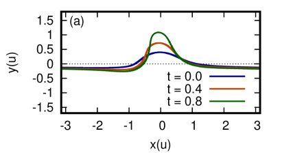
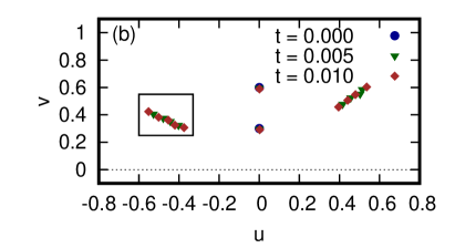
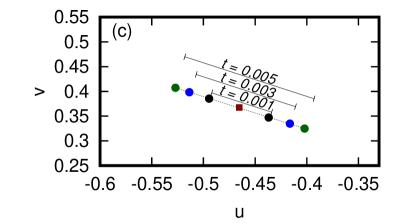
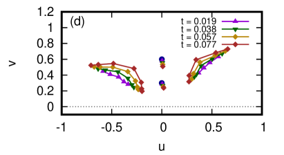
Figure 2: Simulations with the initial conditions (109),(112) and $g=\alpha=0.$ (a) Profiles of free surface at different times. (b) Complex singularities of $z_{u}$ recovered by AGH algorithm at small times including the initial time $t=0.$ Two persistent poles recovered by AGH algorithm are shown by thick dots of different style moving near the imaginary axis. It is seen that these two poles, originating from the initial conditions (their initial positions are exactly at the imaginary axis according to Eq. (112)), only slightly move away from the initial positions at these early times. Two initial zeros of $z_{u}$ located at $w=w_{\pm}$ according to Eq. (113) turn into two short branch cuts at arbitrary short times. Each branch cut connects two branch points. These branch cuts are revealed in AGH algorithm by a dense set of poles located near $w=w_{\pm}$ with the number of these poles growing with time. (c) The schematic zoom into a small area around $w=w_{-}$ (in (b) that area is shown by the rectangular frame around the left branch cut) to display the extension of branch cut with time. The small filled square shows the point $w=w_{-}$. The length of each branch cut grows approximately linearly with time. (d) The same as in (b) but at larger times when the length of branch cuts reaches $\sim 1.$ Poles approximating branch cuts are connected by solid lines.

Figure 3a and 3b demonstrate that the residues of both $z_{u}$ and $\Pi_{u}$ are the integrals of motions for $g=0$ fully confirming the analytical results of Eqs. (70) and (71). Figure 3c zooms into trajectories of motion of poles $w=a_{1}(t)$ and $w=a_{2}(t)$ in $w$ plane. Figure 3d shows a time dependence of the pole positions $w=a_{1}(t)$ and $w=a_{2}(t)$ and compares it with the result of the time integration of Eq. (63). The difference between analytical curves and numerical ones are nearly visually indistinguishable. For that comparison $U$ was calculated numerically at each moment of time from $R$ and $V$ by using the definition (30) and applying AGH algorithm to recover $U_{0}(t)$ ($U_{0}$ is defined in Eq. (61)). Only at larger times, when the distance from the branch cuts to either $a_{1}$ or $a_{2}$ turns comparable with the spacing between poles approximating branch cut in AGH algorithm, the difference between analytical and numerical values becomes noticeable as expected from the discussion of Section 8.2.

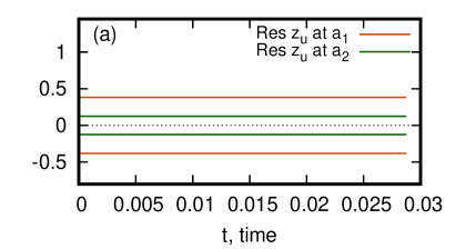
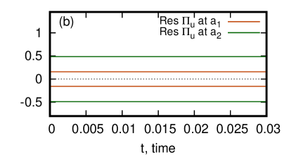
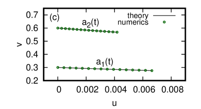
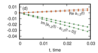
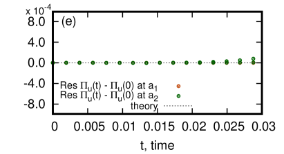
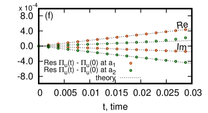
Figure 3: (a) The residues of $z_{u}$ at $w=a_{1}(t)$ and $w=a_{2}(t)$ as functions of $t$ compared with Eq. (70). (b) The residues of $\Pi_{u}$ at $w=a_{1}(t)$ and $w=a_{2}(t)$ compared with Eq. (71). (c) Trajectories of $w=a_{1}(t)$ and $w=a_{2}(t)$ in $w$ plane compared with the result of the integration of the analytical expression (63). (d) A dependence of real and imaginary parts of $a_{1}$ and $a_{2}$ on $t$ for the same data as in (b). (a)-(d) is shown for the same simulation as in Figure 2 (with $g=0$). (e) and (f) are the same type of plots as as (a) and (b) except a nonzero gravity $g=0.04$ is added in the simulation with all other parameters the same as in the simulations of Figure 2.

Assuming $g=0.04$ with all other numerical parameters as above, we obtain simulation results similar to shown in Figure 2  because the simulation time remains relatively small so that the effect of nonzero $g$ is small for free surface profiles. However, the residue of $\Pi_{u}$ is not constant any more but attains the linear dependence on time as follows from Eq. (71). Then Figures 3a and 3b (the case $g=0$) are replaced by new Figures 3e and 3f (the case $g=0.04).$ There is again the excellent agreement between simulations and the theoretical curves given by Eqs. (70) and (71).

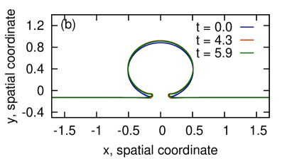
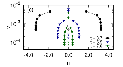
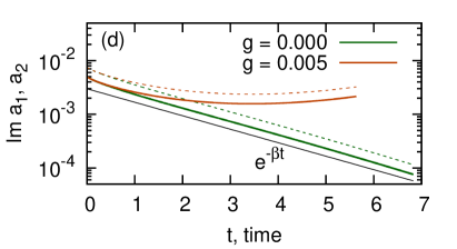
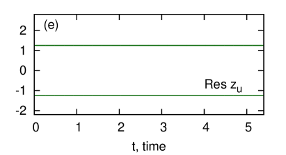
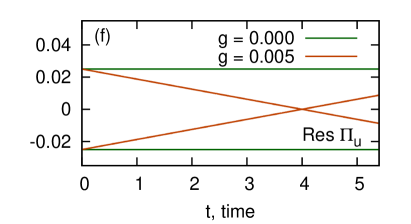
Figure 4: Simulations with the initial conditions (109),(114) and $\alpha=0.$ (a) and (b): profiles of free surface at different times for $g=0$ and $g=0.005$, respectively. (c) Positions of two persistent poles (originate at $w=a_{1}(0)$ and $w=a_{2}(0),$ shown by small open circles, triangles and rhombus) and branch cuts (thick dots and triangles connected by solid lines) are shown at different $t$ for simulation with $g=0.$ These poles and branch cuts determine the mushroom type shape of (a). There are other branch cuts well above (not shown) which determine only a background of the free surface height outside of the mushroom. (d) Vertical positions for both poles (solid and dashed lines) for $g=0$ and $g=0.005$ vs. $t$ in log scale. The exponential dependence $\propto e^{-\beta t}$, $\beta\simeq 0.578329$ is also shown for the comparison. (e) The residues of $z_{u}$ at $w=a_{1}(t)$ and $w=a_{2}(t)$ extracted from the simulations are constant in time both for $g=0$ and $g=0.005$ in agreement with Eq. (70). (f) The residues of $\Pi_{u}$ at $w=a_{1}(t)$ and $w=a_{2}(t)$ are either constant or liner function of $t$ depending on $g$ and are visually indistinguishable from Eq. (71).

We now consider the initial conditions (109) for another set of numerical values

$$a_{1}(0)=0.0050\,\mathrm{i},\,a_{2}(0)=0.0075\,\mathrm{i},\ q=1.25\mathrm{i},\,c=0.02.$$ (114)

Eqs. (9.1) and (114) result in $w_{+}=0.0790677\ldots+\mathrm{i}\,0.00625\ldots\quad\text{and}\quad w_{-}=-0.0790677\ldots+\mathrm{i}\,0.00625\ldots,$ i.e. $w_{\pm}\in\mathbb{C}^{+}$ in this case as required. Similar to the previous simulations description of this section, Taylor series expansion of $z_{u}$ and $\Pi_{u}$ (109) at $w=w_{\pm}\in\mathbb{C}^{+}$ and $t=0$ reproduces Eqs. (44) and (45) in the variables $R$ and $V$ with $R_{-1}\neq 0$ and $V_{-1}\neq 0$. Then Theorem 1 of Section 3 proves that solutions (44) and (45) are not persistent in time. At $w=w_{\pm}$ we again expect a formation of a pair of square root branch points at arbitrary small time $t>0$. The initial poles at $w=a_{1}(0)$ and $w=a_{2}(0)$ are expected to be persistent for at least a finite time duration according to the results of Section 4.

Figure 4a shows profiles of free surface at various times obtained from simulations of Dyachenko Eqs. (30), (32), (33), (35) and (36) with the initial conditions (109),(114) and $g=\alpha=0.$ Figures  4b shows a simulation with the same parameters except $g=0.005$ and $\alpha=0.$ It is seen at Figures 4a and  4b that the inial free surface has a form of disk standing on the nearly flat surface. Then this disk moves upwards with almost constant velocity (for $g=0$) forming a mushroom with a narrow neck (stipe). For $g=0.005$ that upward motion is quickly suppressed by the nonzero gravity. Figures  4c demonstrate both a persistence in time of two poles originating from $w=a_{1}(0),\ w=a_{2}(0)$ and a self-similar dynamics of branch cuts originating from $w=w_{\pm}.$ Figure 4d shows a time dependence of position of two poles moving strictly in the vertical direction. Contrary to the previous numerical example, both poles are never absorbed into branch cut and they are persistent at all times. Figure 4e and 4f demonstrate that the dynamics of residues of both $z_{u}$ and $\Pi_{u}$ is in full agreement with Eqs. (70) and (71) both for $g=0$ and $g\neq 0.$ Log-linear scaling of Figure 4c also demonstrates that at large time an d $g=0$ both poles and surrounding branch cuts evolve in a self-similar way (if we rescale with time both $u$ and $v$) approaching the real line with a spatial scaling $\propto e^{-\beta t}$, where $\beta\simeq 0.578329$ is obtained from the numerical fit of the curves of Figure  4d.

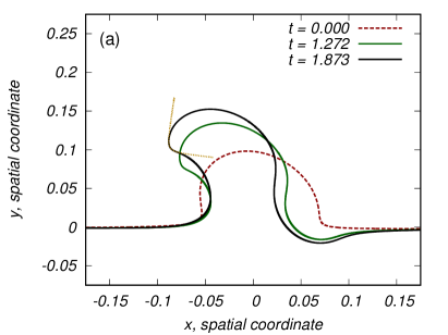
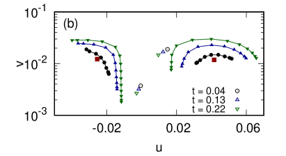
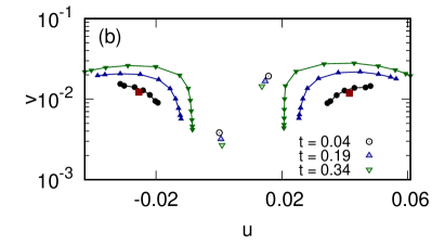
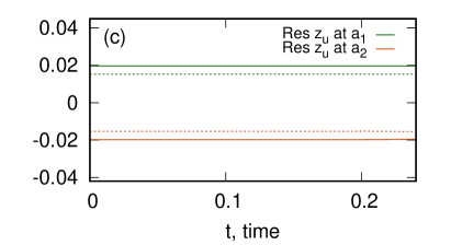
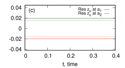
Figure 5: Simulations of the initial conditions (109),(115), $g=\alpha=0$ and either (116) (left panels) or (117) (right panels). (a) The shape of the surface. Dotted line on the left panel shows a fit of the overturning portion of the wave to the square root dependence $z=q\,(w-w_{c})^{1/2}+z_{0}$, where fitting parameters are $z_{0}=0.0923+0.0961\,\mathrm{i}$ and $q=0.595329+4.48567\,\mathrm{i}$ while $w_{c}=-0.02348+3.2923\cdot 10^{-6}\,\mathrm{i}$ is recovered from AGH algorithm as the position the lowest end of the branch cut. (b) A motion of poles (small open circles and triangles) and branch cuts (filled circles and triangles connected by solid lines) in $w$ plane. The small filled squares show the point $w=w_{\pm}$ from Eq. (9.1). (c) Residues of $z_{u}$ extracted from simulations are constant in time in agreement with Eq. (70). A similar statement is true for residues of $\Pi_{u}$ in accordance with Eq. (71) (not shown).

Two more sets of the initial conditions (109) have initial poles away from the imaginary axis and are given by

$$a_{1}(0)=0.004\,\mathrm{i},\,a_{2}(0)=0.016+0.020\,\mathrm{i},\ q=0.025e^{\mathrm{i}0.71\pi}$$ (115)

with either

$$c=0.03-0.02\mathrm{i}$$ (116)

or

$$c=0.02.$$ (117)

Eqs. (9.1) and (115) result in $w_{+}=0.0415052\ldots+\mathrm{i}\,0.0117937\ldots\quad\text{and}\quad w_{-}=-0.0255052\ldots+\mathrm{i}\,0.0122063\ldots,$ i.e. $w_{\pm}\in\mathbb{C}^{+}$ in these cases as required. Figure 5a shows jets propelled in the direction oblique to the imaginary axis which is more pronounced in the case (116) (left panel in Figure 5a). The initial poles at $w=a_{1}(0)$ and $w=a_{2}(0)$ are again persistent in time with residues obeying Eqs. (70)and (71) as shown in Figures 5b and 5c. Also a fit to the square root dependence shown on left Figure 5a by a dotted line corresponds to the square root branch point at the lowest end of the left branch cut as seen in Figure 5b.

9.2 Simulations with second order poles

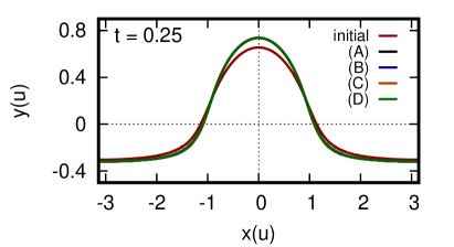
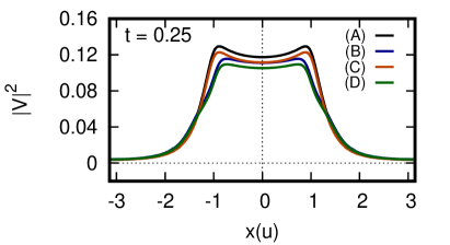
Figure 6: (Left) Free surface profiles resulting from simulations for the cases (A), (B), (C) and (D) of Eq. (124) at $t=0.25$ compared with the initial profile at $t=0.$ (Right) $|V|^{2}$ at the free surface for the same cases.

Consider an initial condition in the form of the second order pole at $w=a(0)$ both in $z_{u}$ and $\Pi_{u}$ as follows

$$z_{u} =1+\frac{q}{\cos(w-a(0))-1}=1-\frac{q(\zeta^{2}+1)}{2\cos^{2}\frac{a}{2}(\zeta-\tan\frac{a}{2})^{2}},$$ (118)

$$\Pi_{u} =\mathrm{i}c(1-z_{u}),$$ (119)

where $a(0)\in\mathbb{C}^{+},$ $c\neq 0,q\neq 0\in\mathbb{C}$ are the constants and we used the identity (110).

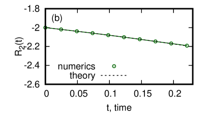
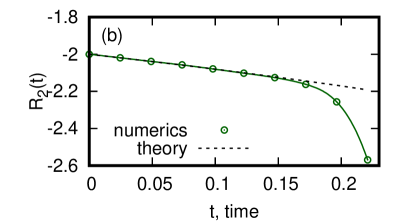
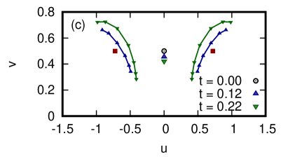
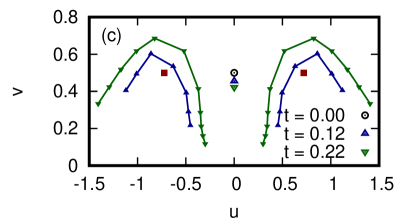
Figure 7: Data extracted from simulations for the cases (A) (left panels) and (B) (right panels) of Eq. (124). (a) A dependence of $Im(a)$ on $t$ in Eq. (97) compared with the result of the integration of the analytical expression (91) ($a$ is purely imaginary in these cases). For each moment of time the location of $w=a=\mathrm{i}Im(a)$ was found as the solution of $R(w)=0$ by the Newton’s method. (b) A dependence of $R_{2}$ on $t$ in Eq. (97) compared with the result of the integration of the analytical expression (94). $R_{2}$ is purely real in these cases. In both (a) and (b), $U_{0}(t)$ and $U_{1}(t)$ were obtained from AGH algorithm similar to Section 9.1. (c) Motion of the pole (small open circle and triangles) and branch cuts (filled triangles connected by solid lines) in $w$ plane for $z(w,t)$. The small filled squares show the points $w=w_{\pm}$ from Eq. (123).

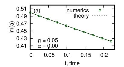
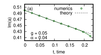
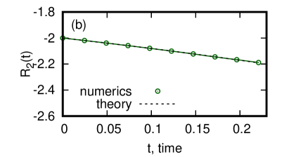
Figure 8: Similar results to Figure 7a and 7b but for the cases (C) (left panels) and (D) (right panels) of Eq. (124).

The initial conditions (118) and (119) together with Eqs. (37) and (38) imply that both $R$ and $V$ are analytic at $w=a(0)$ for $t=0$ with their Taylor series coefficients satisfying

$$R_{0}(0)=R_{1}(0)=R_{3}(0)=0,\ R_{2}(0)=-\frac{1}{2q}\neq 0,V_{0}(0)=c\neq 0,\ V_{1}(0)=0,$$

$$V_{2}(0)=\frac{c}{2q}\ \text{at}\ w=a$$ (120)

for $t=0.$ Thus $R$ has a second order zero while $V$ is nonzero at $w=a(0)$ provided $q\neq 0$ and $c\neq 0$ which corresponds to the case of Eqs. (89) and (90). Then the analytical results of Section 6 predict a persistence of second order poles at $w=a(t)$ of both $z_{u}$ and $\Pi_{u}$ for at least a finite duration of time for arbitrary values of $g$ and $\alpha$. We study four separate cases $g=\alpha=0;g=0,\alpha\neq 0;g\neq 0,\alpha=0;g\neq 0,\alpha\neq 0.$

The conformal map (1) requires that $z_{u}\neq 0$ for $w\in\mathbb{C}^{-}$. Solving for $z_{u}=0$ in Eq. (118) results in

$$w_{\pm}=2\arctan\left[\frac{2A\pm(1+A^{2})\sqrt{q(2-q)}}{2-q[A^{2}+1]}\right],\quad A\equiv\tan{\frac{a(0)}{2}}$$ (121)

which provides a restriction on allowed numerical values of $q$ and $a(0)$ to ensure that $w_{\pm}\in\mathbb{C}^{+}.$

We choose numerical values

$$c=0.5,\quad q=0.25\quad\text{and}\quad a(0)=0.5\mathrm{i}$$ (122)

for all four cases. Eqs. (121) and (122) result in

$$w_{+}=0.722734\ldots+\mathrm{i}\,0.5\quad\text{and}\quad w_{-}=-0.722734\ldots+\mathrm{i}\,0.5,$$ (123)

i.e. $w_{\pm}\in\mathbb{C}^{+}$ in this case as required. Taylor series expansion of $z_{u}$ and $\Pi_{u}$ (109) at $w=w_{\pm}\in\mathbb{C}^{+}$ and $t=0$ reproduces Eqs. (44) and (45) in the variables $R$ and $V$ with $R_{-1}\neq 0$ and $V_{-1}\neq 0$. Then Theorem 1 of Section 3 proves that solutions (44) and (45) are not persistent in time. Similar to the discussion of Section 9.1, we expect a formation of a pair of square root branch points at an arbitrary small time $t>0$.

Figures 6a and  6b show profiles of free surface and $|V|^{2}$ obtained from simulations of Dyachenko Eqs. (30), (32), (33), (35) and (36) with the initial conditions (118),(119),(122) and four particular cases

$$(A)g=\alpha=0;\ (B)g=0,\,\alpha=0.04;\ (C)g=0.05,\alpha=0;\ \text{and}\ (D)g=0.05,\alpha=0.04.$$ (124)

Figures  7a and 7b show time dependencies of the second order pole of both $z_{w}(w,t)$ and $\Pi_{w}(w,t)$ at $w=a(t)$ as well as the coefficient $R_{2}(t)$ of Taylor series (89) (also enter into Eqs. (97)) compared with a time integration of Eqs. (91) and (94). It confirms a persistence in time of second order poles originating from $w=a(0)$ for the initial conditions (118) and (119). We also recovered $V_{1}(t)$ from simulations (not shown in Figures) which together with $R_{2}(t)$ allowed to confirm the integral of motion (96).

Figure 7c shows the positions of complex singularities of $z$ in the complex plane $w\in\mathbb{C}.$ The branch cuts form at arbitrary small time $t>0$ from the points $w=w_{\pm}$ (123). It is seen that the nonzero surface tension on the right panel of Figure 7c results in a significantly faster extension of these branch cuts compared with the zero surface tension case on the left panel. This is consistent with the results of Ref. Dyachenko & Newell (2016) that an addition of surface tension results in quick approach of singularities to the real line. Similar to simulations of Section 9.1, at larger times the poles start absorbing into branch cuts. The deviation between analytical and numerical results in right panels of Figures 7a and 7b at later times is due to the faster approach of branch cuts to the pole position for $\alpha\neq 0$ thus resulting in AGH algorithm to loose the numerical precision as expected from the discussion of Section 8.2. We also note that our use of $z$ (instead of using $z_{u}$ in Section 9.1) to obtain Figures 7a-7c is due to the convenience of recovering simple poles in AGH algorithm compared with the second order poles. Indeed, $z$ has the first order pole at $w=a$ as obtained from the integration of Eq. (97) over $w$. Generally such integration produces also a logarithmic branch point $w=a$ from the simple pole in Eq. (97) which would imply a formation of multiple poles approximating that branch point by AGH algorithm in Figure 7c. However, the particular initial conditions (118) and (119) imply through Eqs. (96),(98)-(100),(9.2) that $V_{1}(t)=R_{3}(t)=0,$ i.e. $\underset{w=a}{Res}(\Pi_{w})=\underset{w=a}{Res}(z_{w})=0$ thus removing a logarithmic branch point $w=a.$ The absence a logarithmic branch point $w=a$ in Figure 7c also provides another confirmation of the persistence of the second order pole in $z_{u}$ at $w=a$ and the validity of the motion integrals (96) and (98)-(100).

Figure 8 shows results similar Figures  7a and 7b but with $g\neq 0.$ The positions of complex singularities are not shown because they are nearly the same as in Figure  7c.

We conclude that in this section we verified with a high numerical precision a conservation of both complex integrals of motion of Section 4 and all three independent complex integrals of motions for the second order pole case of Section 6.

10 Conclusion and Discussion

The main result of this paper is the existence of new integrals of motion in free surface hydrodynamics. These integrals are closely tied to the existence of solutions with poles of the first and the second orders in both $z_{w}$ and $\Pi_{w}.$ The residues of $z_{w}$ are the integral of motion while residues of $\Pi_{w}$ are the linear function of time for nonzero gravity turning into the integrals of motion for zero gravity. The residues of $z_{w}$ at different points commute with each other in the sense of underlying non-canonical Hamiltonian dynamics. It provides an argument in support of the conjecture of complete integrability of free surface hydrodynamics in deep water. We also suggested to treat the analytical continuation of the free surface dynamics outside of the physical fluid as the phantom hydrodynamics on the multi-sheet Riemann surface. That phantom hydrodynamics allows a generalized Kelvin theorem. We expect that generally a number of sheets will be infinite with generic solutions to involve poles and square root branch points in multiple sheets.

For future work we suggest an extension to the general case of the poles of arbitrary order in $z_{w}$ and $\Pi_{w}$ to count the total number of independent integrals of motion. We propose to also study the expected pole solutions in other (nonphysical) sheets of Riemann surface. The commutativity properties between different integral of motion need to be studied in the general case.

11 Acknowledgements.

The work of A.I.D., P.M.L. and V.E.Z. was supported by the state assignment “Dynamics of the complex systems ”. The work of P.M.L. was supported by the National Science Foundation, grant DMS-1814619. The work of S.A.D. was supported by the National Science Foundation, grant number DMS-1716822. The work of V.E.Z. was supported by the National Science Foundation, grant number DMS-1715323. The work of A.I.D. and V.E.Z. described in sections 2, 3 and 6 was supported by the Russian Science Foundation, grant number 19-72-30028.

References

- Alpert et al. (2000) Alpert, Bradley, Greengard, Leslie & Hagstrom, Thomas 2000 Rapid evaluation of nonreflecting boundary kernels for time-domain wave propagation. SIAM J. Num. Anal. 37, 1138–1164.
- Arnold (1989) Arnold, V. I. 1989 Mathematical Methods of Classical Mechanics. Springer.
- Baker et al. (1993) Baker, Gregory, Caflisch, Russel E. & Siegel, Michael 1993 Singularity formation during Rayleigh–Taylor instability. Journal of Fluid Mechanics 252, 51–78.
- Baker et al. (1982) Baker, Gregory R., Meiron, Daniel I. & Orszag, Steven A. 1982 Generalized vortex methods for free-surface flow problems. Journal of Fluid Mechanics 123, 477–501.
- Baker & Shelley (1990) Baker, G. R. & Shelley, M. J. 1990 On the connection between thin vortex layers and vortex sheets. Journal of Fluid Mechanics 215, 161–194.
- Baker & Xie (2011) Baker, Gregory R. & Xie, Chao 2011 Singularities in the complex physical plane for deep water waves. J. Fluid Mech. 685, 83–116.
- Boyd (2001) Boyd, J. P. 2001 Chebyshev and Fourier Spectral Methods: Second Revised Edition. Dover Publications.
- Caflisch & Orellana (1989) Caflisch, R. & Orellana, O. 1989 Singular Solutions and Ill–Posedness for the Evolution of Vortex Sheets. SIAM Journal on Mathematical Analysis 20 (2), 293–307.
- Caflisch et al. (1990) Caflisch, R., Orellana, O. & Siegel, M. 1990 A Localized Approximation Method for Vortical Flows. SIAM Journal on Applied Mathematics 50 (6), 1517–1532.
- Caflisch et al. (1993) Caflisch, Russel E., Ercolani, Nicholas, Hou, Thomas Y. & Landis, Yelena 1993 Multi-valued solutions and branch point singularities for nonlinear hyperbolic or elliptic systems. Communications on Pure and Applied Mathematics 46 (4), 453–499.
- Chalikov & Sheinin (1998) Chalikov, D. & Sheinin, D. 1998 Direct modeling of one-dimensional nonlinear potential waves. Adv. Fluid Mech 17, 207–258.
- Chalikov & Sheinin (2005) Chalikov, D. & Sheinin, D. 2005 Modeling of extreme waves based on equation of potential flow with a free surface. Journal of Computational Physics 210, 247–273.
- Chalikov (2016) Chalikov, Dmitry V. 2016 Numerical Modeling of Sea Waves. Springer.
- Cowley et al. (1999) Cowley, Stephen J., Baker, Greg R. & Tanveer, Saleh 1999 On the formation of Moore curvature singularities in vortex sheets. J. Fluid Mech. 378, 233–267.
- Crowdy (2002) Crowdy, D. G. 2002 On a class of geometry-driven free boundary problems. SIAM. J. Appl. Math. 62, 945–954.
- Dubrovin et al. (1985) Dubrovin, B. A., Fomenko, A. T. & Novikov, S. P. 1985 Modern Geometry: Methods and Applications: Part II: The Geometry and Topology of Manifolds. Springer.
- Dyachenko (2001) Dyachenko, Alexander I. 2001 On the dynamics of an ideal fluid with a free surface. Dokl. Math. 63 (1), 115–117.
- Dyachenko et al. (2013a) Dyachenko, A. I., Kachulin, D. I. & Zakharov, V. E. 2013a On the nonintegrability of the free surface hydrodynamics. JETP Letters 98, 43–47.
- Dyachenko et al. (1996) Dyachenko, Alexander I., Kuznetsov, Evgenii A., Spector, Michael & Zakharov, Vladimir E. 1996 Analytical description of the free surface dynamics of an ideal fluid (canonical formalism and conformal mapping). Phys. Lett. A 221, 73–79.
- Dyachenko et al. (2019) Dyachenko, A. I., Lushnikov, P. M. & Zakharov, V. E. 2019 Non-canonical Hamiltonian structure and Poisson bracket for two-dimensional hydrodynamics with free surface. Journal of Fluid Mechanics 869, 526–552.
- Dyachenko & Zakharov (1994) Dyachenko, Alexander I. & Zakharov, Vladimir E. 1994 Is free surface hydrodynamics an integrable system? Phys. Lett. A 190 (2), 144–148.
- Dyachenko & Newell (2016) Dyachenko, Sergey & Newell, Alan C. 2016 Whitecapping. Stud. Appl. Math. 137, 199–213.
- Dyachenko et al. (2013b) Dyachenko, Sergey A., Lushnikov, Pavel M. & Korotkevich, Alexander O. 2013b The complex singularity of a Stokes wave. JETP Letters 98 (11), 675–679.
- Dyachenko et al. (2016) Dyachenko, Sergey A., Lushnikov, Pavel M. & Korotkevich, Alexander O. 2016 Branch Cuts of Stokes Wave on Deep Water. Part I: Numerical Solution and Padé Approximation. Studies in Applied Mathematics 137, 419–472.
- G. A. Baker & Graves-Morris (1996) G. A. Baker, Jr. & Graves-Morris, P. R. 1996 Padé Approximants, 2nd ed.,. Cambridge: Cambridge Univ. Press.
- Gardner et al. (1967) Gardner, Clifford S., Greene, John M., Kruskal, Martin D. & Miura, Robert M. 1967 Method for Solving the Korteweg-deVries Equation. Phys. Rev. Lett. 19, 1095.
- Gonnet et al. (2011) Gonnet, Pedro, Pachon, Ricardo & Trefethen, Lloyd N. 2011 Robust rational interpolation and least-squares. Electronic Transactions on Numerical Analysis 1388, 146–167.
- Grant (1973) Grant, Malcolm A. 1973 The singularity at the crest of a finite amplitude progressive Stokes wave. J. Fluid Mech. 59(2), 257–262.
- Karabut & Zhuravleva (2014) Karabut, E. A. & Zhuravleva, E. N. 2014 Unsteady flows with a zero acceleration on the free boundary. J. Fluid Mech. 754, 308–331.
- Krasny (1986) Krasny, Robert 1986 A study of singularity formation in a vortex sheet by the point–vortex approximation. Journal of Fluid Mechanics 167, 65–93.
- Kuznetsov et al. (1993) Kuznetsov, E.A., Spector, M.D. & Zakharov, V.E. 1993 Surface singularities of ideal fluid. Physics Letters A 182 (4-6), 387 – 393.
- Kuznetsov et al. (1994) Kuznetsov, E. A., Spector, M. D. & Zakharov, V. E. 1994 Formation of singularities on the free surface of an ideal fluid. Phys. Rev. E 49, 1283–1290.
- Lamb (1945) Lamb, H. 1945 Hydrodynamics. Dover Books on Physics.
- Landau & Lifshitz (1989) Landau, L. D. & Lifshitz, E. M. 1989 Fluid Mechanics, Third Edition: Volume 6. New York: Pergamon.
- Lushnikov & Zubarev (2018) Lushnikov, P.M. & Zubarev, N.M. 2018 Exact solutions for nonlinear development of a Kelvin-Helmholtz instability for the counterflow of superfluid and normal components of Helium II. Phys. Rev. Lett. 120, 204504.
- Lushnikov (2004) Lushnikov, P. M. 2004 Exactly integrable dynamics of interface between ideal fluid and light viscous fluid. Physics Letters A 329, 49 – 54.
- Lushnikov (2016) Lushnikov, Pavel M. 2016 Structure and location of branch point singularities for Stokes waves on deep water. Journal of Fluid Mechanics 800, 557–594.
- Lushnikov et al. (2017) Lushnikov, Pavel M., Dyachenko, Sergey A. & Silantyev, Denis A. 2017 New conformal mapping for adaptive resolving of the complex singularities of Stokes wave. Proc. Roy. Soc. A 473, 20170198.
- Meiron et al. (1982) Meiron, Daniel I., Baker, Gregory R. & Orszag, Steven A. 1982 Analytic structure of vortex sheet dynamics. Part 1. Kelvin–Helmholtz instability. Journal of Fluid Mechanics 114, 283–298.
- Meison et al. (1981) Meison, D., Orzag, S. & Izraely, M. 1981 Applications of numerical conformal mapping. J. Comput. Phys. 40, 345–360.
- Mineev-Weinstein et al. (2000) Mineev-Weinstein, Mark, Wiegmann, Paul B & Zabrodin, Anton 2000 Integrable structure of interface dynamics. Phys. Rev. Lett. 84 (22), 5106–5109.
- Moore (1979) Moore, D. W. 1979 The spontaneous appearance of a singularity in the shape of an evolving vortex sheet. Proceedings of the Royal Society of London A: Mathematical, Physical and Engineering Sciences 365 (1720), 105–119.
- Novikov et al. (1984) Novikov, S., Manakov, S. V., Pitaevskii, L. P. & Zakharov, V. E. 1984 Theory of Solitons: The Inverse Scattering Method. Springer.
- Ovsyannikov (1973) Ovsyannikov, Lev V. 1973 Dynamics of a fluid. M.A. Lavrent’ev Institute of Hydrodynamics Sib. Branch USSR Ac. Sci. 15, 104–125.
- Richardson (1972) Richardson, S. 1972 Hele Shaw flows with a free boundary produced by the injection of fluid into a narrow channel. Journal of Fluid Mechanics 56, 609–618.
- Shelley (1992) Shelley, M. J. 1992 A study of singularity formation in vortex–sheet motion by a spectrally accurate vortex method. Journal of Fluid Mechanics 244, 493–526.
- Stokes (1847) Stokes, George G. 1847 On the theory of oscillatory waves. Transactions of the Cambridge Philosophical Society 8, 441–455.
- Stokes (1880) Stokes, George G. 1880 On the theory of oscillatory waves. Mathematical and Physical Papers 1, 197–229.
- Tanveer (1991) Tanveer, S. 1991 Singularities in water waves and Rayleigh-Taylor instability. Proc. R. Soc. Lond. A 435, 137–158.
- Tanveer (1993) Tanveer, S. 1993 Singularities in the classical Rayleigh-Taylor flow: formation and subsequent motion. Proc. R. Soc. Lond. A 441, 501–525.
- Weinstein (1983) Weinstein, A. 1983 The local structure of Poisson manifolds. J. Differential Geometry 18, 523–557.
- Zakharov (1968) Zakharov, Vladimir E. 1968 Stability of periodic waves of finite amplitude on a surface. J. Appl. Mech. Tech. Phys. 9 (2), 190–194.
- Zakharov & Dyachenko (2012) Zakharov, Vladimir E. & Dyachenko, Alexander I. 2012 Free-surface hydrodynamics in the conformal variables , arXiv: 1206.2046.
- Zakharov et al. (2002) Zakharov, Vladimir E., Dyachenko, Alexander I. & Vasiliev, Oleg A. 2002 New method for numerical simulation of nonstationary potential flow of incompressible fluid with a free surface. European Journal of Mechanics B/Fluids 21, 283–291.
- Zakharov & Faddeev (1971) Zakharov, V. E. & Faddeev, L. D. 1971 Korteweg-de Vries equation: A completely integrable Hamiltonian system. Functional Analysis and Its Applications 5, 280–287.
- Zakharov & Shabat (1972) Zakharov, V. E. & Shabat, A. B. 1972 Exact theory of 2-dimensional sef-focusing and one-dimensional self-modulation of waves in nonlinear media. Sov. Phys. JETP 34, 62.
- Zubarev (2000) Zubarev, N M 2000 Charged-surface instability development in liquid helium: An exact solution. JETP Lett. 71, 367–369.
- Zubarev (2002) Zubarev, N M 2002 Exact solutions of the equations of motion of liquid helium with a charged free surface. J. Exp. Theor. Phys. 94, 534–544.
- Zubarev (2008) Zubarev, N. M. 2008 Formation of Singularities on the Charged Surface of a Liquid-Helium Layer with a Finite Depth. Journal of Experimental and Theoretical Physics 107, 668–678.
- Zubarev & Karabut (2018) Zubarev, N. M. & Karabut, E. A. 2018 Exact Local Solutions for the Formation of Singularities on the Free Surface of an Ideal Fluid. JETP Letters 107, 412–417.
- Zubarev & Kuznetsov (2014) Zubarev, N M & Kuznetsov, E A 2014 Singularity Formation on a Fluid Interface During the Kelvin-Helmholtz Instability Development. J. Exp. Theor. Phys. 119, 169–178.