Critical behavior in graphene: spinodal instability at room temperature

Abstract

At a critical spinodal in-plane stress $\tau_{C}$ a planar crystalline graphene layer becomes mechanically unstable. We present a model of the critical behavior of the membrane area near $\tau_{C}$ and show that it is in complete agreement with path-integral simulations and with recent experiments based on interferometric profilometry and Raman spectroscopy. Close to the critical stress, $\tau_{C}$, the in-plane strain behaves as $\left(\tau_{C}-\tau\right)^{1/2}$ for $\tau<\tau_{C}$.

Since the first experimental characterization of graphene as a two-dimensional (2D) one-atom thick solid membrane,(Novoselov et al., 2004, 2005) a huge amount of experimental and theoretical work has been devoted to this material.(Amorim et al., 2014; Roldan et al., 2017) The very existence of a crystalline 2D membrane was unexpected from general symmetry arguments by the Mermin-Wagner theorem.(Mermin and Wagner, 1966) The surface corrugation of the layer was considered as an important mechanism for the modification of its electronic properties(Deng and Berry, 2016) as well as an stabilizing factor for the planar morphology of the layer.(Fasolino et al., 2007)

A well-known model to explain the stabilization of the planar layer assumes that the amplitude of the out-of-plane fluctuations follows a power-law, i.e., $\left\langle h^{2}\right\rangle\varpropto N^{1-(\eta/2)}$, with $N$ being the number of atoms in the sheet, and $\eta$ an anomalous exponent $\eta\sim 0.8-0.85$.(Doussal and Radzihovsky, 2018) The anharmonic coupling between the out-of-plane and in-plane phonon modes increases the bending rigidity of the layer, so that for long wavelengths the bending constant becomes dependent on the wavevector as $\kappa(k)\propto k^{-\eta}$. The theoretical framework for this model is the self-consistent screening approximation (SCSA) applied to a tensionless membrane, that also predicts that the membrane should display a negative Poisson ratio, $\nu=-1/3$.(Doussal and Radzihovsky, 2018) Several classical simulations of out-of-plane fluctuations of graphene have been analyzed by following this theoretical model.(Fasolino et al., 2007; Los et al., 2016; Hašík et al., 2018) However, to the best of our knowledge there is no experimental confirmation that the behavior of graphene is described by an anomalous exponent $\eta\sim 0.8-0.85$. On the contrary, there are experimental data(Politano et al., 2012) and computer simulations(Los et al., 2016) supporting that the Poisson ratio of a graphene layer is positive $(\nu\sim 0.16)$ and differs from the predicted auxetic value of $\nu=-1/3$.

Recent analytical investigations offer an alternative explanation for the stability of the planar morphology of the layer. By a perturbational treatment of anharmonicity, it is predicted that free-standing graphene displays a small but finite acoustic sound velocity in the out-of-plane direction, caused by the bending of the layer. (Adamyan et al., 2016; Bondarev et al., 2018) Similar results were derived by different analytical perturbational approaches.(Amorim et al., 2014; Michel et al., 2015) A finite sound velocity $v$ implies that the free-standing layer displays a finite surface tension, $\sigma=\rho v^{2},$ where $\rho$ is the density of the layer. The surface tension $\sigma$ acts as an intrinsic tensile stress that is responsible for the observed stability of a planar graphene layer. Classical(Ramírez and Herrero, 2017) and quantum(Herrero and Ramírez, 2018) simulations of free-standing graphene are in excellent agreement with the theory presented in Refs. Adamyan et al., 2016 and Bondarev et al., 2018.

Relevant physical information on the intrinsic stability of a planar layer can be gained by studying the approach to its limit of mechanical stability. In recent papers(Ramírez and Herrero, 2017, 2018) we have shown that at a critical compressive in-plane stress $\tau_{C}$ a planar graphene layer becomes mechanically unstable. At this applied stress $\tau_{C}$, the flat membrane is unstable against long-wavelength bending fluctuations. For $\tau>\tau_{C}$ the layer forms wrinkles, i.e., periodic and static undulations, with amplitudes several orders of magnitude larger than those arising from thermal fluctuations. Such wrinkles have been often observed experimentally.(Bao et al., 2009; Hattab et al., 2012; Bao et al., 2012; Zhang et al., 2013; Bai et al., 2014; Deng and Berry, 2016; Meng et al., 2013) The purpose of this work is to give a simple model of the critical behavior of the planar layer close to $\tau_{C}$. We compare this model with quantum simulations of a free-standing layer and confirm its validity by the agreement to experiments that monitored the strain of the layer through two complementary techniques: interferometric profilometry and Raman spectroscopy.(Nicholl et al., 2017)

Quantum path-integral molecular-dynamics (PIMD) simulations of graphene are performed as a function of the applied in-plane stress $\tau$ at temperature $T=$ 300 K.(Ceperley, 1995; Herrero and Ramírez, 2014) The empirical interatomic LCBOPII model was employed for the calculation of interatomic forces and potential energy.(Los et al., 2005) The simulations were done in the $N\tau T$ ensemble with full fluctuations of the simulation cell.(Tuckerman, 2002) The simulation cell contains $N=960$ carbon atoms and 2D periodic boundary conditions were applied. The in-plane stress $\tau$ is the lateral force per unit length at the boundary of the simulation cell. All results presented here correspond to a planar (i.e. not wrinkled) morphology of the membrane. Technical details of the quantum simulations are identical to those reported in our previous studies of graphene and are not repeated here.(Herrero and Ramírez, 2016, 2017, 2018; Ramírez and Herrero, 2018)

Our simulations at 300 K focus on the dependence of the membrane area with the applied in-plane stress $\tau$. The area of the 2D simulation cell is $NA_{p}$, $A_{p}$ being the in-plane area per atom. The pair ($A_{p},\tau)$ are thermodynamic conjugate variables.(Fournier and Barbetta, 2008; Tarazona et al., 2013) In addition, the real area $NA$ was estimated by triangulation of the surface, which six triangles filling each hexagon of the lattice. The six triangles share the barycenter of the hexagon as a common vertex. The physical significance of the real area $A$ of the membrane can be inferred from recent experiments using x-ray photoelectron (XPS)(Pozzo et al., 2011) and Raman spectroscopy.(Nicholl et al., 2017) This area $A$ is related to the average covalent CC distance while the in-plane area $A_{p}$ yields the average in-plane lattice constant. The difference between both has been referred earlier as the hidden area of the membrane.(Nicholl et al., 2015, 2017) An ongoing discussion in the field of lipid bilayer membranes is that their thermodynamic properties should be better described using the notion of a real area $A$ rather than its in-plane projection $A_{p}$.(Fournier and Barbetta, 2008; Waheed and Edholm, 2009; Chacón et al., 2015) The real area and the negative surface tension ($A,-\sigma$) are a pair of conjugate variables. (Fournier and Barbetta, 2008; Tarazona et al., 2013)

The surface tension $\sigma$ determines the long-wavelength limit of the acoustic bending modes (ZA) of the layer. The dispersion relation of the ZA modes in this limit can be described as(Ramírez et al., 2016)

$$\rho\omega^{2}=\sigma k^{2}+\kappa k^{4},\;$$ (1)

where $k$ is the module of the wavevector and isotropy in the 2D $k-$space is assumed. Numerical details of the Fourier analysis of the amplitude of the out-of-plane atomic fluctuations to obtain the parameters $\sigma$ and $\kappa$ from computer simulations, are given in Ref. Ramírez et al., 2016. At constant temperature, the surface tension $\sigma$ and the in-plane stress $\tau$ of the planar layer are related as:(Ramírez et al., 2016; Ramírez and Herrero, 2017)

$$\sigma=\sigma_{0}-\tau,$$ (2)

where $\sigma_{0}$ is the surface tension for vanishing in-plane stress. From the Fourier analysis of atomic trajectories in PIMD simulations, one derives $\sigma_{0}\sim 0.1$ N/m at 300 K.(Ramírez and Herrero, 2018)

For a layer made of $N$ atoms, the bending mode with largest wavelength (or smallest $k$ module) is $k_{N}=2\pi/(NA_{p})^{1/2}$. The critical surface tension, $\sigma_{C}$ , corresponds to the appearance of a soft bending mode with wavenumber $\omega(k_{N})=0$. Taking into account Eqs. (1) and (2),

$$\sigma_{C}=-\kappa k_{N}^{2}=\sigma_{0}-\tau_{C}\>.$$ (3)

The critical surface tension displays a significant finite size effect, $\sigma_{C}\propto N^{-1}$. It vanishes ($\sigma_{C}=0)$ in the thermodynamic limit. Meanwhile the critical in-plane stress displays a compressive positive value $\tau_{C}=\sigma_{0}$ in this limit.

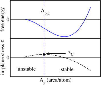
Figure 1: Sketch of the dependence of the Helmholtz free energy and the in-plane stress of a solid membrane as a function of its projected area. At the critical (spinodal) point the in-plane stress takes on its maximum compressive value, $\tau_{C}$. The spinodal point is the limit for the mechanical stability of a planar membrane. $\tau_{C}$ displays a size effect as described by Eq. (3) in the main text.

The physical origin of the bending instability at $\tau_{C}$ can be understood on a common basis with other critical phenomena in condensed matter, e.g., cavitation of liquid helium and sublimation of noble-gas solids under tensile stress.(Maris, 1991; Boronat et al., 1994; Bauer et al., 2000; Herrero, 2003) For any solid membrane at a given temperature the free energy $F$ depends on the in-plane surface area $A_{p}$ as displayed qualitatively in Fig. 1. If a compressive stress ($\tau>0)$ is applied the in-plane area $A_{p}$ decreases. However, since the in-plane stress $\tau=-dF/dA_{p}$ has a maximum at the inflection point of $F$ vs $A_{p}$, there is an upper limit to the compressive stress the planar layer can sustain. At this spinodal stress, $\tau_{C,},$ $d^{2}F/dA_{p}^{2}=0$ and from a Taylor expansion of the free energy at the spinodal area, $A_{p,C}$, one gets for $\tau<\tau_{C}$

$$\tau-\tau_{C}\varpropto-(A_{p}-A_{p,C})^{2}\>.$$ (4)

The critical behavior of the in-plane area $A_{p}$ implies a nonlinear stress-strain relation. Here the stress is a quadratic function of the strain. Note that the critical in-plane stress, $\tau_{C},$ depends on the finiteness of the graphene sample, as can be seen from Eq. (3).

The real surface area $A$ depends on the average distance of strong covalent CC bonds.(Pozzo et al., 2011) The long wavelength bending of the layer does not critically change neither the covalent distance nor the real area $A$ of the membrane.(Ramírez and Herrero, 2018) One expects here a Hooke’s law:

$$\tau-\tau_{C}\varpropto-(A-A_{C})\>,$$ (5)

where $A_{C}$ is the real area at the spinodal point.

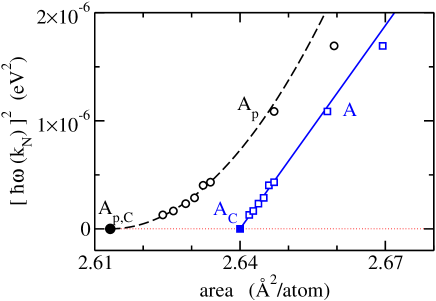
Figure 2: Square of the energy quantum of the bending mode with wavevector $k_{N}$ vs. the in-plane (open circles) and the real area (open squares) of the membrane at 300 K. The wavevector $k_{N}$ correspond to the bending mode with the longest wavelength in the simulation cell. The wavenumber vanishes $(\omega=0$) at the critical (spinodal) point. The broken line is a quadratic fit of $\left(\hbar\omega\right)^{2}$ for $A_{p}<2.64$ $\textrm{\AA}^{2}$/atom. The full line is a linear fit of $\left(\hbar\omega\right)^{2}$ for $A<2.65$ $\textrm{\AA}^{2}$/atom. The critical areas ($A_{p,C}$ and $A_{C}$) obtained from the fits are represented as full symbols.

The critical values $A_{p,C}$ and $A_{C}$ were obtained from the PIMD simulations in the following way. For the wavevector with smallest module in the simulation cell, $k_{N}$, one gets according to Eqs. (1$-$3):

$$\omega{}^{2}\propto-(\tau-\tau_{C})\>.$$ (6)

The results of $\left(\hbar\omega\right)^{2}$ for the wavevector $k_{N}$ derived at 300 K are plotted in Fig. 2. The values correspond to simulations at several in-plane stresses in the range $0.4>\tau>-1$ N/m. The squared energies $\left(\hbar\omega\right)^{2}$ are shown as a function of the projected area $A_{p}$ (open circles), and as a function of the real area $A$ (open squares). As the layer is compressed, the area of the membrane and the phonon energy, $\hbar\omega$, decrease and approach the critical point.

At the critical (spinodal) point, the wavenumber of the bending mode vanishes ($\omega=0$). The quadratic fit of $\left(\hbar\omega\right)^{2}$, performed in the region where $A_{p}<$ 2.64 $\textrm{\AA}^{2}$/atom, is displayed as a broken line in Fig. 2. The vertex of the parabola corresponds to the critical in-plane area: $A_{p,C}=2.613$ $\textrm{\AA}^{2}$/atom. The linear fit of $\left(\hbar\omega\right)^{2}$, performed in the region $A<$ 2.65 $\textrm{\AA}^{2}$/atom, is plotted by a full line in Fig. 2. The extrapolated value of the real area at the spinodal point is $A_{C}=2.64$ $\textrm{\AA}^{2}$/atom. Near the critical point, $(\hbar\omega)^{2}$ varies linearly with the in-plane stress $\tau$ [see Eq. (6)]. The value of the critical stress derived from this dependence is $\tau_{C}=0.5$ N/m (see Fig. 4 of Ref. Ramírez and Herrero, 2018).

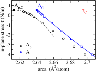
Figure 3: Simulation results for the in-plane stress as a function of the in-plane area $A_{p}$ (open circles) and as a function of the real area $A$ (open squares). Close to the spinodal tension, $\tau_{C},$ the state equation $\tau(A_{p})$ is a parabola (broken line) with its vertex at the critical point. For large tensile stresses ($\tau<-0.5$ N/m) the simulation results for $\tau(A_{p})$ (open circles) lie in a curve nearly parallel to $\tau(A)$. The full line for $\tau(A)$ is a guide to the eye.

The critical values, $\tau_{C}$ and $A_{p,C}$, are helpful data to analyze the equation of state $\tau(A_{p})$ of graphene as derived from the simulations. The function $\tau(A_{p})$ is displayed in Fig. 3 as open circles. The result resembles the sketch displayed in Fig. 1. The broken line is a quadratic f it using the critical point (closed circle) and the open circles with $A_{p}<$ 2.64 $\textrm{\AA}^{2}$/atom. The critical point ($A_{p,C},\tau_{C}$) is the vertex of the parabola. The parabola provides an excellent description of the equation of state for stresses within the critical region $\tau_{C}>\tau>\tau_{C}-1\;\textrm{N/m}$.

In Fig. 3, the simulation results for $\tau(A$) (open squares) follow a linear Hooke’s law, as expected from Eq. (5). At large tensile stresses ($\tau<-0.5$ N/m), i.e., outside the critical region, the functions $\tau(A_{p})$ (open circles) and $\tau(A$) (full line) are nearly parallel. The equation of state $\tau(A_{p})$ displays a crossover from a non-Hookean quadratic behavior in the critical region ($\tau\gtrsim-0.5$ N/m) to a Hookean linear behavior at larger tensile stresses ($\tau\lesssim-0.5$ N/m).

The crossover in the equation of state $\tau(A_{p})$ is a result that should be reproduced by other simulations of graphene. In fact, the curves $\tau(A_{p})$ derived at 300 K by classical Monte Carlo simulations (see Fig.2 of Ref. Los et al., 2016) seems to agree with our analysis. Also recent simulations on a BN monolayer display a critical behavior entirely similar to the one described here for graphene.(Calvo and Magnin, 2016) More important is that the equations of state derived from the simulations, $\tau(A_{p})$ and $\tau(A)$, can be directly compared with recent experiments. Stress-strain curves of free-standing graphene were obtained by two complementary techniques: interferometric profilometry and Raman spectroscopy.(Nicholl et al., 2017) These techniques are complementary in the sense that they are applied to the same sample but interferometric profilometry measures the strain $\epsilon_{Int}$ corresponding to the in-plane area $A_{p}$, while Raman spectroscopy measures the strain $\epsilon_{Ram}$ corresponding to the real area $A$.(Nicholl et al., 2017) With the purpose of comparison to the experiments, we define the linear strains from our simulation data as

$$\epsilon_{Ap}=\frac{(A_{p}-A_{p,C})}{2A_{P.C}}\>;\>\epsilon_{A}=\frac{(A-A_{C})}{2A_{C}}\>.$$ (7)

The factor 2 in the denominator converts surface into linear strain. Here the stress is measured as the surface tension referred to its critical value

$$\sigma_{rel}=\sigma-\sigma_{C}=-(\tau-\tau_{C})\>.$$ (8)

We have considered the experimental stress-strain curves of samples A and B of Ref. Nicholl et al., 2017. The graphene samples have an unknown built-in stress. Thus the two experimental stress-strain curves, $\epsilon_{Int}(\sigma)$ and $\epsilon_{Ram}(\sigma)$, of a given sample have been shifted along the horizontal axis by a constant stress. The experimental curves $\epsilon_{Int}$($\sigma)$ were fitted to the critical relation given by Eq. (4)

$$\epsilon_{Int}(\sigma)=D(\sigma-\sigma_{C})^{1/2}\>,$$ (9)

where $D$ and $\sigma_{C}$ are fitting constants. The result for $\sigma_{C}$ is 0.16 N/m for sample A and 0.1 N/m for sample B.

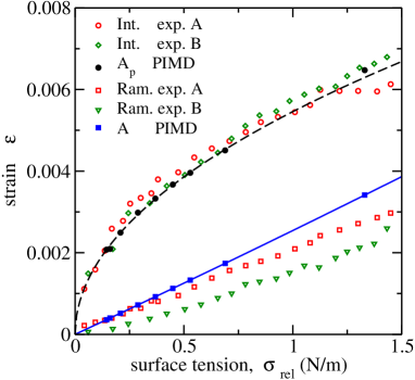
Figure 4: Open symbols are experimental stress-strain curves for samples A and B from Ref. Nicholl et al., 2017. The experimental strain was monitored by interferometric profilometry (Int.) and Raman spectroscopy (Ram.) The experimental stress of sample A was shifted by a adding a constant of $-0.16$ N/m, and those of sample B by $-0.1$ N/m. The strains derived from PIMD simulations are shown as closed circles for the in-plane area $A_{p}$, and as closed squares for the real area $A$. The broken line is the analytical stress-strain curve corresponding to the parabola (broken line) in Fig. 3. The full line is a guide to the eye.

The shifted experimental curves, $\epsilon_{Int}$($\sigma_{rel})$ and $\epsilon_{Ram}$($\sigma_{rel})$, for samples A and B are shown in Fig. 4 as open symbols.(Nicholl et al., 2017) The PIMD result for $\epsilon_{Ap}(\sigma_{rel})$ (closed circles) displays a nearly quantitative agreement to the experimental data in Fig. 4. The difference between simulation and experiment is of the same order as the difference between the experimental results of specimens A and B. The broken line in Fig. 4 corresponds to the state points described by the critical parabola (broken line) in Fig. 3. The strain measured by interferometric profilometry $\epsilon_{Int}$ covers the whole critical region of the planar layer. The critical behavior of the in-plane area is the physical explanation for the strong nonlinearity of the experimental $\epsilon_{Int}$ curves. In our simulations, the critical behavior of $\epsilon_{Ap}$ is solely due to the thermal fluctuations of flexural phonons. In real graphene devices, the presence of static wrinkles would cause an additional increase in the measured strain $\epsilon_{Int}$. This might be a reason to explain the stress-strain curve for a third sample C in the experiments by Nicholl et al., whose strain is shifted with respect to those of samples A and B towards higher values.(Nicholl et al., 2017)

The $\epsilon_{Ram}(\sigma_{rel})$ curves are nearly linear. The inverse slope $d\sigma_{rel}/d\epsilon_{Ram}=2B$ is proportional to the 2D modulus of hydrostatic compression, $B$, of the layer. $B$ is defined by the inverse of the compressibility of the real surface area $A$.(Ramírez and Herrero, 2017) The 2D compressional modulus $B$ predicted by the employed potential model is somewhat smaller than that derived from the experimental $\epsilon_{Ram}(\sigma_{rel})$ curves.

Summarizing, we have given a simple model of the critical behavior of a planar graphene layer close to the compressive stress at which it becomes unstable. The excellent agreement between stress-strain curves derived from the model, from PIMD simulations, and from previous experiments, provides insight into the mechanical properties of a free-standing graphene layer. The high-quality experimental stress-strain results of Ref. Nicholl et al., 2017 can be quantitatively explained by the effect of the applied stress on the equilibrium thermal fluctuations of the layer area at room temperature.