Consistent derivation of the Hawking effect for both non-extremal and extremal Kerr black holes

Abstract

It is believed that extremal black holes do not emit Hawking radiation as understood by taking extremal limits of non-extremal black holes. However, it is debated whether one can make such conclusion reliably starting from an extremal black hole, as the associated Bogoliubov coefficients which relate ingoing and outgoing field modes do not satisfy the required consistency condition. We address this issue in a canonical approach firstly by presenting an exact canonical derivation of the Hawking effect for non-extremal Kerr black holes. Subsequently, for extremal Kerr black holes we show that the required consistency condition is satisfied in the canonical derivation and it produces zero number density for Hawking particles. We also point out the reason behind the reported failure of Bogoliubov coefficients to satisfy the required condition.

I Introduction

In a landmark article Hawking (1975), Hawking pioneered the idea of black hole radiation. In particular, by considering quantum fields in static, charged or rotating black hole spacetimes, he showed that the asymptotic observers would perceive thermal particle creation which is referred to as the Hawking effect. In order to derive the Hawking effect, he used ingoing and outgoing null coordinates for describing the scalar field modes. In last four decades the Hawking effect has been an extensively studied topic of modern physics. However, there are some related issues which are still debated, particularly involving the case of extremal black holes.

It is usually believed that extremal black holes do not exhibit Hawking radiation as one would conclude by taking the extremal limits of non-extremal black holes. However, whether one can make such conclusion starting from an extremal black hole is still debated in the literature Vanzo (1997); Liberati et al. (2000); Alvarenga et al. (2003a, b). These debates stem from the fact that the associated Bogoliubov transformation coefficients that relate the ingoing and the outgoing field modes do not satisfy the required consistency relation arising from the commutator brackets between the creation and annihilation operators of the field modes. Therefore, these Bogoliubov coefficients which are used for computing number density of Hawking quanta, are not reliable. Consequently, for extremal black holes it is an important question to ask whether one could find a fully consistent derivation to conclude about the vanishing Hawking radiation.

In this article, our aims are two fold. Firstly, we show that using the so called near-null coordinates which were introduced for computing Hawking effect in Schwarzschild spacetime Barman et al. (2018), one can perform an exact canonical derivation for non-extremal rotating Kerr black holes. The usage of these near-null coordinates were necessitated due to the fact that null coordinates cannot be used to construct a non-trivial matter field Hamiltonian. Consequently, a Hamiltonian based canonical derivation of the Hawking effect for a Kerr black hole is still missing.

Secondly, for extremal Kerr black holes, we show that the analogous consistency condition which arises from the requirement of the Poisson bracket of field modes and their conjugate momenta be simultaneously satisfied for different observers, is also fulfilled. Further, we show that in the canonical derivation the associated number density operator for the Hawking quanta vanishes for the extremal Kerr black holes. This feature reaffirms that the extremal Kerr black holes do not emit Hawking radiation. Additionally, the canonical derivation of the Hawking effect for Kerr black holes as presented here provide the initial stage for the study of Hawking effect in the context of the so called polymer quantization Ashtekar et al. (2003); Halvorson (2004), a canonical quantization method used in loop quantum gravityAshtekar and Lewandowski (2004); Rovelli (2004); Thiemann (2007). It appears that the existence of a new length scale could substantially affect the Unruh effect Hossain and Sardar (2016a, b); Hossain and Sardar (2015) as well as Hawking effect in Schwarzschild spacetime Barman et al. (2017). However, the question remains whether such claims can be subjected to experimental verification even if in principle. Given Kerr black holes are the only physically viable black holes, the study of Hawking effect for the Kerr black holes in canonical formulation assumes additional importance.

In the section II, we begin with a brief discussion about the Kerr spacetime. In particular, we emphasize that unlike Schwarzschild spacetime a Kerr black hole spacetime has two horizons, of which the outer one is the event horizon. Then we discuss the properties of the corresponding null geodesics and null coordinates. In the section III, we review the key aspects of the canonical formulation. We consider a minimally coupled massless scalar field in a Kerr black hole spacetime. Then we consider two asymptotic observers; one near past null infinity $\mathscr{I}^{-}$ and another near future null infinity $\mathscr{I}^{+}$. Following Barman et al. (2018), we then define the pair of near-null coordinates to be used for canonical derivation. We then construct the Hamiltonian densities associated with the Fourier modes of the field as seen by these two observers. In the section IV, we consider non-extremal Kerr black holes and then present the canonical derivation of the Hawking effect as represented by the thermal distribution of the Hawking quanta. Subsequently, in the section V we study the case for extremal Kerr black holes.

II The Kerr spacetime

The spacetime geometry outside of a rotating black hole is described by the Kerr metric which is an exact vacuum solution of the Einstein equation in general relativity. It is further generalized by the advent of Kerr-Newman metric where one includes a net charge to a rotating black hole. However, it is rather a theoretical construct given a charged astrophysical body is unlikely to be found in nature. On the other hand the abundance of rotating Kerr black holes in our universe and the recent discovery of gravitational waves from their merger Abbott et al. (2016a, b); Abbott et al. (2016c); Abbott et al. (2017) makes them interesting astrophysical objects to investigate further.

II.1 Metric and horizons in Kerr spacetime

The Kerr spacetime is described by two parameters, namely the mass of the black hole $M$ and its angular momentum per unit mass $a$. Using the natural units where speed of light $c$ and Planck constant $\hbar$ are set to unity, one can express the corresponding invariant distance element using Boyer-Lindquist coordinates Boyer and Lindquist (1967) as

$$ds^{2}=-\frac{1}{\rho^{2}}(\Delta-a^{2}\sin^{2}{\theta})dt^{2}+\frac{\rho^{2}}{\Delta}dr^{2}+\rho^{2}d\theta^{2}$$

$$~{}+\frac{\Sigma}{\rho^{2}}\sin^{2}{\theta}~{}d\phi^{2}-\frac{2a}{\rho^{2}}(r^{2}+a^{2}-\Delta)\sin^{2}{\theta}~{}dtd\phi~{},$$ (1)

where $\rho^{2}=r^{2}+a^{2}\cos^{2}{\theta}$, $\Sigma=(r^{2}+a^{2})^{2}-a^{2}\Delta\sin^{2}{\theta}$ and $\Delta=r^{2}+a^{2}-r_{s}r$ with $r_{s}=2GM$ being the Schwarzschild radius corresponding to mass $M$ Kerr (2007); Poisson (2007); Dadhich (2013); Schutz (1985); Raine and Thomas (2005); Carroll (2004); D’Inverno (1992); Padmanabhan (2010); Heinicke and Hehl (2014); Krasinski (1978); Teukolsky (2015); Visser (2007); Smailagic and Spallucci (2010). The metric components diverge at both $\rho^{2}=0$ and $\Delta=0$. In particular, the Kretschmann scalar is singular at $\rho^{2}=0$, which signifies a curvature singularity and cannot be removed by any coordinate transformation. On the other hand, $\Delta=0$ corresponds to a coordinate singularity and it gives the position of two horizons at $r=r_{h}$ and $r=r_{c}$ where

$$r_{h}=\tfrac{1}{2}(r_{s}+\sqrt{r_{s}^{2}-4a^{2}}~{})~{},~{}r_{c}=\tfrac{1}{2}(r_{s}-\sqrt{r_{s}^{2}-4a^{2}}~{})~{}.$$ (2)

The outer horizon, located at $r_{h}$, is the event horizon with the surface gravity $\mathrm{\varkappa}_{h}=\sqrt{r_{s}^{2}-4a^{2}}/(2r_{s}r_{h})$. The inner horizon is located at $r_{c}$ and it is a Cauchy horizon with surface gravity $\mathrm{\varkappa}_{c}=\sqrt{r_{s}^{2}-4a^{2}}/(2r_{s}r_{c})$. Due to the frame-dragging effect Poisson (2007); Schutz (1985), an inertial observer experiences an angular velocity in Kerr spacetime, given by

$$\Omega\equiv\Omega(r,\theta)=\frac{g^{t\phi}}{g^{tt}}=\frac{arr_{s}}{\Sigma}~{}.$$ (3)

We may mention that the study as presented here can be generalized for the Kerr-Newman black holes Newman et al. (1965); Adamo and Newman (2014); Newman and Janis (1965) by using $\Delta=r^{2}+a^{2}+r_{Q}^{2}-r_{s}r$, where $r_{Q}^{2}=Q^{2}G/4\pi\epsilon_{0}$ with charge $Q$ and Coulomb’s force constant $1/4\pi\epsilon_{0}$.

II.2 Null trajectories in Kerr spacetime

In Kerr spacetime the governing equations for null geodesics Poisson (2007) can be expressed as

$$\dot{t}=\frac{r^{2}+a^{2}}{\Delta},~{}\dot{r}=\pm 1~{},~{}\dot{\theta}=0~{},~{}\dot{\phi}=\frac{a}{\Delta}~{},$$ (4)

where the overhead dot denotes derivative with respect to an affine parameter. Due to the frame dragging effect the azimuthal angle $\phi$ cannot be kept constant along any ingoing or outgoing null trajectory, unlike in Schwarzschild spacetime. However, using the Eqn. (4) one can show that along the ingoing null trajectories, the coordinates $v=t+r_{\star}$ and $\psi=\phi+r_{\sharp}$ are constants where

$$dr_{\star}=\frac{r^{2}+a^{2}}{\Delta}dr~{}~{},~{}~{}dr_{\sharp}=\frac{a}{\Delta}dr~{}.$$ (5)

Similarly, along the outgoing null trajectories the coordinates $u=t-r_{\star}$ and $\chi=\phi-r_{\sharp}$ are constants. Here $r_{\star}$ denotes the tortoise coordinate in analogy to the one in Schwarzschild spacetime. Depending on whether the Kerr black hole is extremal or non-extremal, the expression of the coordinates $r_{\star}$ and $r_{\sharp}$ in terms of radial coordinate $r$ differ.

II.3 Number density of Hawking quanta

In order to study the Hawking effect we consider the scenario where Kerr spacetime is formed after the collapse of matters starting from a Minkowski spacetime in the past. The detailed evolution of the collapsing matters are not relevant for our study. To capture this aspect of change in metric over time, yet to avoid the technical difficulties that are associated with the field quantization in a single time-dependent metric, Hawking considered two different asymptotic observers, one at past null infinity $\mathscr{I}^{-}$, and other at future null infinity $\mathscr{I}^{+}$, each having time-independent but different metric. The vacuum states corresponding to these two observers differ from each other as their metric are different.

To represent the Hawking quanta, in the given spacetime with metric $g_{\mu\nu}$, we consider a minimally coupled massless free scalar field $\Phi(x)$ which is described by the action

$$S_{\Phi}=\int d^{4}x\left[-\frac{1}{2}\sqrt{-g}g^{\mu\nu}\nabla_{\mu}\Phi(x)\nabla_{\nu}\Phi(x)\right]~{}.$$ (6)

The Hawking effect is realized by computing the Bogoliubov transformation coefficients between these two observers at the past and the future null infinities respectively. The expectation value of the number density operator corresponding to the Hawking quanta of frequency $\omega$ is given by Hawking (1975)

$$N_{\omega}=\frac{1}{e^{2\pi(\omega-m\Omega_{h})/\mathrm{\varkappa}_{h}}-1}~{},$$ (7)

where $\mathrm{\varkappa}_{h}$ and $\Omega_{h}$ are the surface gravity and the angular velocity $\Omega$ at the event horizon respectively. Here $m$ denotes the azimuthal quantum number of the modes. By comparing the Eqn. (7) with the blackbody distribution we may read off the corresponding Hawking temperature as $T_{H}=\mathrm{\varkappa}_{h}/(2\pi k_{B})$ with $k_{B}$ being the Boltzmann constant.

III canonical formulation

The particle creation in a curved spacetime is directly connected to the dynamical nature of the spacetime metric. In the case of black hole radiation, it arises as the spacetime evolves from being Minkowskian in the past to a specific black hole spacetime in future due to the collapse of matters. In order to perform Hamiltonian based canonical derivation of the Hawking effect in Kerr spacetime we follow a similar approach by considering two asymptotic observers near past and future null infinities, each having time-independent but different metric. Subsequently, we compute expectation value of the Hamiltonian density operator for the field modes of the future observer in the vacuum state of the past observer and then read off the number density of the Hawking quanta.

III.1 Reduced scalar field action

In the Kerr spacetime with axial symmetry, one can decompose the scalar field in terms of spheroidal harmonics $e^{im\phi}\mathscr{S}_{lm}(\theta)$ as $\Phi(x)=\sum_{l,m}e^{im\phi}\mathscr{S}_{lm}(\theta)~{}\varphi_{lm}(r,t)/\sqrt{r^{2}+a^{2}}$. However, in order to emphasize a key aspect of Kerr spacetime we perform the reduction in two steps. Firstly, we express the scalar field as $\Phi(t,r,\theta,\phi)=\sum_{lm}e^{im\phi}~{}\Phi_{lm}(t,r,\theta)$. After carrying out the integration over azimuthal angle $\phi$, the action (6) reduces to $S_{\Phi}=\sum_{ll^{\prime}m}S_{ll^{\prime}m}$ where

$$S_{ll^{\prime}m} = \int dtdrd\theta\sqrt{-g}\left[-\tfrac{1}{2}g^{tt}\partial_{t}\Phi_{l^{\prime}m}^{*}\partial_{t}\Phi_{lm}\right.$$ (8)

$$-~{}~{}\left.\tfrac{i}{2}m~{}g^{t\phi}(\partial_{t}\Phi_{l^{\prime}m}^{*}\Phi_{lm}-\Phi_{l^{\prime}m}^{*}\partial_{t}\Phi_{lm})\right.$$

$$\left.-~{}~{}\tfrac{1}{2}g^{rr}\partial_{r}\Phi_{l^{\prime}m}^{*}\partial_{r}\Phi_{lm}-\tfrac{1}{2}g^{\theta\theta}\partial_{\theta}\Phi_{l^{\prime}m}^{*}\partial_{\theta}\Phi_{lm}\right.$$

$$\left.~{}~{}~{}~{}~{}~{}~{}~{}~{}~{}~{}~{}~{}~{}~{}~{}~{}~{}~{}~{}~{}~{}~{}~{}-\tfrac{1}{2}m^{2}g^{\phi\phi}\Phi_{l^{\prime}m}^{*}\Phi_{lm}\right]~{}.$$

We note that if one redefines the field further as

$$\Phi_{lm}(t,r,\theta)\equiv e^{-im\Omega t}~{}\tilde{\Phi}_{lm}(t,r,\theta)~{},$$ (9)

then the terms in the action (8) involving temporal derivative of fields simplify to

$$S_{ll^{\prime}m} = \int dtdrd\theta\sqrt{-g}\left[-\tfrac{1}{2}g^{tt}\partial_{t}\tilde{\Phi}_{l^{\prime}m}^{*}\partial_{t}\tilde{\Phi}_{lm}\right.$$ (10)

$$-\left.\tfrac{1}{2}g^{rr}\partial_{r}(e^{-im\Omega t}\tilde{\Phi}_{l^{\prime}m})^{*}\partial_{r}(e^{-im\Omega t}\tilde{\Phi}_{lm})\right.$$

$$-\left.\tfrac{1}{2}g^{\theta\theta}\partial_{\theta}(e^{-im\Omega t}\tilde{\Phi}_{l^{\prime}m})^{*}\partial_{\theta}(e^{-im\Omega t}\tilde{\Phi}_{lm})\right.$$

$$-\left.\tfrac{1}{2}m^{2}\left(g^{\phi\phi}-\Omega g^{t\phi}\right)\tilde{\Phi}_{l^{\prime}m}^{*}\tilde{\Phi}_{lm}~{}\right]~{}.$$

In the regions near the past and the future null infinities where the relevant observers for realizing Hawking effect are located, the redefined field can be expressed as $\tilde{\Phi}_{lm}(t,r,\theta)\simeq\mathscr{S}_{lm}(\theta)~{}\varphi_{lm}(r_{\star},t)/\sqrt{r^{2}+a^{2}}$. The same approximation for the field is also possible in the region near the event horizon $\Delta\to 0$ where the term $\Omega$ becomes $\Omega_{h}$ which is the angular velocity of the event horizon. By using orthogonality condition $\int d(\cos{\theta})\mathscr{S}_{lm}(\theta)\mathscr{S}^{*}_{l^{\prime}m}(\theta)=\delta_{l,l^{\prime}}$, we achieve the final form of the reduced action as $S_{\Phi}=\sum_{lm}S_{lm}$ in the regions near horizon as well as near null infinities, where

$$S_{lm}\simeq\int dtdr_{\star}\left[\tfrac{1}{2}\partial_{t}\varphi^{*}_{lm}\partial_{t}\varphi_{lm}-\tfrac{1}{2}\partial_{r_{\star}}\varphi^{*}_{lm}\partial_{r_{\star}}\varphi_{lm}\right]~{}.$$ (11)

The action (11) represents a scalar field in 1+1 dimensional flat spacetime.

III.2 Frequency shift due to frame dragging

The solutions to the field equation corresponding to the action (11) can be expressed as

$$\varphi_{lm}(r,t)\sim\frac{1}{\sqrt{2\pi\tilde{\omega}}}e^{-i\tilde{\omega}(t\pm r_{\star})}~{}.$$ (12)

However, in order to understand the full dynamics of the physical field $\Phi$, one needs to consider the solutions (12) together with the relation (9) which provides additional time-dependence. In particular, if one reads off the frequency, as defined as the eigenvalue of the operator $i\partial_{t}$, then it would be $\tilde{\omega}$ for redefined field mode $\varphi_{lm}$ (12). On the other hand, the frequency, say $\omega$, of the physical field mode $\Phi_{lm}$ (9) would be $\omega=\tilde{\omega}+m\Omega$. The Hawking effect is realized through the modes which travel out from the region very close to the event horizon. Therefore, for these modes the frequency $\tilde{\omega}$ can be related to the physical frequency $\omega$ as Ford (1975); Hod (2011); Menezes (2017, 2018); Lin and Soo (2013); Miao et al. (2012); Iso et al. (2006)

$$\tilde{\omega}=\omega-m\Omega_{h}~{}.$$ (13)

This key feature of frequency shift in the Kerr spacetime is reflected through the expression of the expectation value of the number density operator (7).

III.3 The observers $\mathbb{O}^{-}$ and $\mathbb{O}^{+}$

III.3.1 Near-null coordinates

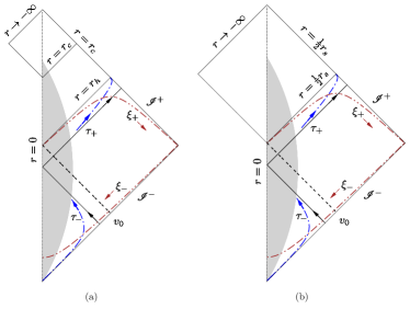
Figure 1: Simplified Penrose diagrams for (a) non-extremal and (b) extremal Kerr black holes. The black hole is formed through matter collapse which is depicted by the shaded region. A null ray leaving from $\mathscr{I}^{-}$ before $v_{0}$ would end up on $\mathscr{I}^{+}$ whereas a null ray leaving after $v_{0}$ would end up being inside the black hole.

The field modes (12) are usually expressed in terms of the null coordinates $v$ and $u$ as $\tilde{\varphi}_{lm}\sim e^{-i\tilde{\omega}v}$ or $\tilde{\varphi}_{lm}\sim e^{-i\tilde{\omega}u}$. Therefore, the Hawking effect is conveniently understood using Bogoliubov transformation coefficients between field modes of the two observers, each are described by null coordinates (see Fig.1). However, the usage of the null coordinates do not lead to a true matter Hamiltonian that can describe the dynamics of these modes. Therefore, in the pursuit of a canonical derivation of the Hawking effect we need to look for coordinates which are not null. By following the approach as prescribed in Barman et al. (2018) we define a set of near-null coordinates by slightly deforming the outgoing and the ingoing null coordinates. In particular, for the observer located near the past null infinity $\mathscr{I}^{-}$, say observer $\mathbb{O}^{-}$, the near-null coordinates are defined as

$$\tau_{-}=t-(1-\epsilon)r_{\star}~{}~{};~{}~{}\xi_{-}=-t-(1+\epsilon)r_{\star}~{},$$ (14)

where the parameter $\epsilon$ is considered to be small such that $\epsilon\gg\epsilon^{2}$. In a similar manner we define the near-null coordinates for the observer located near the future null infinity $\mathscr{I}^{+}$, say observer $\mathbb{O}^{+}$, as

$$\tau_{+}=t+(1-\epsilon)r_{\star}~{}~{};~{}~{}\xi_{+}=-t+(1+\epsilon)r_{\star}~{}.$$ (15)

We are considering the scenario where the black hole is formed after the collapse of matters staring from a Minkowskian spacetime. Therefore, for the past observer $\mathbb{O}^{-}$, the definition of tortoise coordinate in (14) is trivial i.e. $dr_{\star}=dr$. We may note that the timelike characteristics of the coordinates $\tau_{\pm}$ is maintained for the range $0<\epsilon<2$. However, for simplicity here we consider the parameter $\epsilon$ to be small.

III.3.2 Field Hamiltonian

For the past observer $\mathbb{O}^{-}$, the 1+1 dimensional reduced spacetime is described by the Minkowski metric $ds^{2}=-dt^{2}+dr_{\star}^{2}=-dt^{2}+dr^{2}$. Therefore, the invariant line element can be written using near-null coordinates (14) as

$$ds^{2}_{-}=\tfrac{\epsilon}{2}[-d\tau_{-}^{2}+d\xi_{-}^{2}+\tfrac{2}{\epsilon}d\tau_{-}d\xi_{-}]\equiv\tfrac{\epsilon}{2}~{}g^{0}_{\mu\nu}dx_{-}^{\mu}dx_{-}^{\nu}~{},$$ (16)

where flat metric $g^{0}_{\mu\nu}$ is conformally transformed. With respect to the future observer $\mathbb{O}^{+}$, the Kerr black hole is already formed. Nevertheless, as far as the dynamics of the 1+1 dimensional reduced scalar field action (11) is concerned, even for the observer $\mathbb{O}^{+}$, the underlying metric can be expressed as $ds^{2}=-dt^{2}+dr_{\star}^{2}$. Using the near-null coordinates (15), this invariant line-element becomes

$$ds^{2}_{+}=\tfrac{\epsilon}{2}[-d\tau_{+}^{2}+d\xi_{+}^{2}+\tfrac{2}{\epsilon}d\tau_{+}d\xi_{+}]\equiv\tfrac{\epsilon}{2}~{}g^{0}_{\mu\nu}dx^{\mu}_{+}dx^{\nu}_{+}~{}.$$ (17)

Therefore, we may express the reduced scalar field action (11) for both observers as

$$S_{\varphi}=\int d\tau_{\pm}d\xi_{\pm}\left[-\tfrac{1}{2}\sqrt{-g^{0}}g^{0\mu\nu}\partial_{\mu}\varphi\partial_{\nu}\varphi\right]~{}.$$ (18)

For brevity of notation we have omitted the subscripts from the redefined field $\varphi_{lm}$.

In order to derive the scalar field Hamiltonian, we consider spatial slicing of the reduced spacetime labelled by the coordinate $\tau_{\pm}$. From Eqns. (16) and (17), one can show that corresponding lapse function $N=1/\epsilon$, shift vector $N^{1}=1/\epsilon$ and determinant of the spatial metric $q=1$. The scalar field Hamiltonian then can be written as

$$H_{\varphi}^{\pm}=\int d\xi_{\pm}\;\tfrac{1}{\epsilon}\left[\left\{\tfrac{1}{2}\Pi^{2}+\tfrac{1}{2}(\partial_{\xi_{\pm}}\varphi)^{2}\right\}+\Pi~{}\partial_{\xi_{\pm}}\varphi\right]~{},$$ (19)

where the superscript $(\pm)$ refers to the Hamiltonian for the observer $\mathbb{O}^{+}$ and $\mathbb{O}^{-}$ respectively. The field $\varphi$ and its conjugate momentum $\Pi$ satisfy the Poisson bracket

$$\{\varphi(\tau_{\pm},\xi_{\pm}),\Pi(\tau_{\pm},\xi_{\pm}^{\prime})\}=\delta(\xi_{\pm}-\xi_{\pm}^{\prime})~{}.$$ (20)

Using Hamilton’s equation, the field momentum $\Pi$ can be expressed as

$$\Pi(\tau_{\pm},\xi_{\pm})=\epsilon\;\partial_{\tau_{\pm}}\varphi-\partial_{\xi_{\pm}}\varphi~{}.$$ (21)

We note from the Eqn. (19) that at the value of the parameter $\epsilon=0$, the Hamiltonian becomes ill-defined. This signifies the necessity of near-null coordinates in order to study the Hawking effect using a Hamiltonian approach.

III.3.3 Fourier modes

For both the observers, the spatial volume $V_{\pm}=\int d\xi_{\pm}\sqrt{q}$ formally diverges as $\sqrt{q}=1$. Therefore to avoid dealing with explicitly diverging quantities, we consider a finite fiducial box during the intermediate steps of computations, such that

$$V_{\pm}=\int_{\xi_{\pm}^{L}}^{\xi_{\pm}^{R}}d\xi_{\pm}\sqrt{q}={\xi_{\pm}^{R}}-{\xi_{\pm}^{L}}~{}.$$ (22)

Subsequently, we define the respective Fourier modes of the scalar field for the observers $\mathbb{O}^{+}$ and $\mathbb{O}^{-}$ as

$$\varphi(\tau_{\pm},\xi_{\pm}) = \tfrac{1}{\sqrt{V_{\pm}}}\sum_{k}\tilde{\phi}^{\pm}_{k}e^{ik\xi_{\pm}}~{},$$

$$\Pi(\tau_{\pm},\xi_{\pm}) = \tfrac{1}{\sqrt{V_{\pm}}}\sum_{k}\sqrt{q}~{}\tilde{\pi}^{\pm}_{k}e^{ik\xi_{\pm}}~{},$$ (23)

where $\tilde{\phi}^{\pm}_{k}=\tilde{\phi}^{\pm}_{k}(\tau_{\pm})$, $\tilde{\pi}^{\pm}_{k}=\tilde{\pi}^{\pm}_{k}(\tau_{\pm})$ are the complex-valued mode functions. The finite volume of the fiducial box leads to the definition of Kronecker delta and Dirac delta as $\int d\xi_{\pm}\sqrt{q}e^{i(k-k^{\prime})\xi_{\pm}}=V_{\pm}\delta_{k,k^{\prime}}$ and $\sum_{k}e^{ik(\xi_{\pm}-\xi_{\pm}^{\prime})}=V_{\pm}\delta(\xi_{\pm}-\xi_{\pm}^{\prime})/\sqrt{q}$ . The definition of these two deltas together imply $k\in\{k_{s}\}$ where $k_{s}=2\pi s/V_{\pm}$ with $s$ being a nonzero integer. These definitions help us to express the scalar field Hamiltonians (19) in terms of the Fourier modes as $H_{\varphi}^{\pm}=\sum_{k}\tfrac{1}{\epsilon}\left(\mathcal{H}_{k}^{\pm}+\mathcal{D}_{k}^{\pm}\right)$ where the Hamiltonian densities and diffeomorphism generators are

$$\mathcal{H}_{k}^{\pm}=\tfrac{1}{2}\tilde{\pi}^{\pm}_{k}\tilde{\pi}^{\pm}_{-k}+\tfrac{1}{2}k^{2}\tilde{\phi}^{\pm}_{k}\tilde{\phi}^{\pm}_{-k}~{},$$ (24)

and

$$\mathcal{D}_{k}^{\pm}=-\tfrac{ik}{2}(\tilde{\pi}^{\pm}_{k}\tilde{\phi}^{\pm}_{-k}-\tilde{\pi}^{\pm}_{-k}\tilde{\phi}^{\pm}_{k})~{},$$ (25)

respectively. The corresponding Poisson brackets are

$$\{\tilde{\phi}^{\pm}_{k},\tilde{\pi}^{\pm}_{-k^{\prime}}\}=\delta_{k,k^{\prime}}~{}.$$ (26)

III.4 Relation between Fourier modes

In order to find relations between the field modes and their conjugate momenta for the two observers, we note that $\varphi(\tau_{-},\xi_{-})=\varphi(\tau_{+},\xi_{+})$, given the field is scalar. The field momentum follows a relation $\Pi(\tau_{+},\xi_{+})=(\partial\xi_{-}/\partial\xi_{+})\Pi(\tau_{-},\xi_{-})$ Barman et al. (2018). A simple way to understand this relation is as follows. In order to realize the Hawking effect, the past observer considers ingoing modes with null coordinate $v$ constant whereas the future observer considers the outgoing modes with null coordinate $u$ constant. Using these restrictions together with expressions of the momenta (21), one can arrive at the given relation between the two momenta. Having these relations between the field and the field momentum, one can obtain the relations between their Fourier modes and respective conjugate momenta as

$$\tilde{\phi}^{+}_{\kappa}=\sum_{k}\tilde{\phi}^{-}_{k}F_{0}(k,-\kappa)~{};~{}\tilde{\pi}^{+}_{\kappa}=\sum_{k}\tilde{\pi}^{-}_{k}F_{1}(k,-\kappa)~{},$$ (27)

where we have considered Fourier modes on fixed spatial hyper-surfaces. The coefficient functions $F_{n}(k,\kappa)$ are given by

$$F_{n}(k,\kappa)=\frac{1}{\sqrt{V_{-}V_{+}}}\int d\xi_{+}\left(\tfrac{\partial\xi_{-}}{\partial\xi_{+}}\right)^{n}~{}e^{ik\xi_{-}+i\kappa\xi_{+}}~{},$$ (28)

where $n=0,1$. These coefficient functions are analogous to the Bogoliubov coefficients in the covariant formulation. In particular we note that for $k,\kappa>0$ the coefficient functions $F_{n}(-k,-\kappa)$ are analogous to the Bogoliubov mixing coefficients $\beta_{\omega\omega^{\prime}}$ whereas $F_{n}(k,-\kappa)$ are analogous to the Bogoliubov coefficients $\alpha_{\omega\omega^{\prime}}$ of Hawking (1975). Using representation of Dirac delta distribution $\delta(\mu)=\tfrac{1}{2\pi}\int dx~{}e^{i\mu x}$ and by setting $\mu=1$, $x=(\pm k\xi_{-}+\kappa\xi_{+})$ there one can obtain a relation

$$F_{1}(\pm k,\kappa)=\mp\left(\tfrac{\kappa}{k}\right)F_{0}(\pm k,\kappa)~{}.$$ (29)

In other words, the evaluation of only one coefficient function, say $F_{0}(\pm k,\kappa)$, is sufficient for the subsequent analysis.

III.5 Poisson bracket consistency condition

The requirement that two different Poisson brackets $\{\tilde{\phi}^{-}_{k},\tilde{\pi}^{-}_{-k^{\prime}}\}=\delta_{k,k^{\prime}}$ and $\{\tilde{\phi}^{+}_{\kappa},\tilde{\pi}^{+}_{-\kappa^{\prime}}\}=\delta_{\kappa,\kappa^{\prime}}$ be simultaneously satisfied, demands a relation between the coefficient functions $F_{0}(\pm k,\kappa)$. In particular, by using the Eqn. (29), we may express this consistency requirement as

$$\mathbb{S}_{-}(\kappa)-\mathbb{S}_{+}(\kappa)=1~{},$$ (30)

where $\mathbb{S}_{\pm}(\kappa)=\sum_{k>0}(\kappa/k)|F_{0}(\pm k,\kappa)|^{2}$. This condition is analogous to the consistency condition between Bogoliubov coefficients Alvarenga et al. (2003b) which arises from the imposition of the commutator bracket between the creation and annihilation operators of the field modes for two asymptotic observers.

III.6 Relation between Hamiltonian densities and diffeomorphism generators

Using relations (27) and (29) one can express the Hamiltonian density $\mathcal{H}_{\kappa}^{+}$ for the observer $\mathbb{O}^{+}$ in terms of the Hamiltonian density $\mathcal{H}_{k}^{-}$ of the observer $\mathbb{O}^{-}$ as

$$\mathcal{H}_{\kappa}^{+}=h_{\kappa}^{1}+\sum_{k>0}\left(\frac{\kappa}{k}\right)^{2}\left[\right|F_{0}(-k,\kappa)|^{2}+|F_{0}(k,\kappa)|^{2}]~{}\mathcal{H}_{k}^{-}~{},$$ (31)

where $h_{\kappa}^{1}=\sum_{k\neq k^{\prime}}(\kappa^{2}/2kk^{\prime})F_{0}(k,-\kappa)F_{0}(-k^{\prime},\kappa)\{\tilde{\pi}^{-}_{k}\tilde{\pi}^{-}_{-k^{\prime}}+kk^{\prime}\tilde{\phi}^{-}_{k}\tilde{\phi}^{-}_{-k^{\prime}}\}$. $h_{\kappa}^{1}$ is being linear in $\phi^{-}_{k}$ and its conjugate momentum, the vacuum expectation value of its quantum counterpart vanishes. Similarly, the diffeomorphism generators of the two observers can be related as

$$\mathcal{D}_{\kappa}^{+}=d_{\kappa}^{1}+\sum_{k>0}\left(\frac{\kappa}{k}\right)^{2}\left[\right|F_{0}(-k,\kappa)|^{2}+|F_{0}(k,\kappa)|^{2}]~{}\mathcal{D}_{k}^{-}~{},$$ (32)

where $d_{\kappa}^{1}=\sum_{k\neq k^{\prime}}(i\kappa^{2}/2k)~{}\{F_{0}(-k,\kappa)F_{0}(k^{\prime},-\kappa)~{}\tilde{\pi}^{-}_{-k}\tilde{\phi}^{-}_{k^{\prime}}-F_{0}(k,-\kappa)F_{0}(-k^{\prime},\kappa)~{}\tilde{\pi}^{-}_{k}\tilde{\phi}^{-}_{-k^{\prime}}\}$ which is also linear in field mode and its conjugate momentum.

III.7 Fock quantization and the vacuum state

The scalar field under consideration is real-valued which imposes condition on the Fourier modes as $\tilde{\phi}^{*}_{k}=\tilde{\phi}_{-k}$. This implies that the real and imaginary parts of field modes are not independent. A suggested way to implement this reality condition is to suitably redefine real and imaginary parts for different domains in terms of a real-valued mode function Hossain et al. (2010); Barman et al. (2018) which leads the Hamiltonian density to represent a simple harmonic oscillator as

$$\mathcal{H}_{k}^{\pm}=\frac{1}{2}\pi^{2}_{k}+\frac{1}{2}k^{2}\phi^{2}_{k}~{},~{}~{}~{}\{\phi^{2}_{k},\pi^{2}_{k^{\prime}}\}=\delta_{k,k^{\prime}}~{},$$ (33)

where $\phi_{k}$ and $\pi_{k}$ are the redefined real-valued field modes. Further, this redefinition makes diffeomorphism generator to vanish i.e. $\mathcal{D}_{k}^{-}=0$.

The Fock quantization of massless free scalar field can be viewed as the Schrödinger quantization of only positive frequency oscillator modes. We may now restrict ourselves with the modes where $k,\kappa>0$ so that the mode frequency can be identified as $\tilde{\omega}=\kappa$ and so on. The energy spectrum for each of these oscillator modes is given by $\hat{\mathcal{H}}_{k}^{-}|n_{k}\rangle=(\hat{N}_{k}^{-}+\tfrac{1}{2})k|n_{k}\rangle=(n+\tfrac{1}{2})k|n_{k}\rangle$ where $\hat{N}_{k}^{-}$ is the corresponding number operator, $|n_{k}\rangle$ are its eigen-states with integer eigenvalues $n\geq 0$. The Hawking effect is realized by computing the expectation value of the Hamiltonian density operator $\hat{\mathcal{H}}_{\kappa}^{+}\equiv(\hat{N}_{\kappa}^{+}+\tfrac{1}{2})$ corresponding to the observer $\mathbb{O}^{+}$ in the vacuum state $|0_{-}\rangle=\Pi_{k}|0_{k}\rangle$ corresponding to the observer $\mathbb{O}^{-}$. Therefore, the expectation value of the number density operator corresponding to the Hawking quanta of frequency $\tilde{\omega}=\kappa$, after using the Eqn. (30) along with the Eqn. (31), can be expressed as

$$N_{\tilde{\omega}}=N_{\kappa}\equiv\langle 0_{-}|\hat{N}_{\kappa}^{+}|0_{-}\rangle=\mathbb{S}_{+}(\kappa)~{},$$ (34)

where we have used the properties $\langle 0_{k}|\hat{\phi}_{k}|0_{k}\rangle=0$ and $\langle 0_{k}|\hat{\pi}_{k}|0_{k}\rangle=0$. For Fock quantization, the number density operator employed in Barman et al. (2018) is equivalent to the number density operator (34).

IV Non-extremal Kerr black holes

In order to explicitly evaluate the coefficient function $F_{0}(k,\kappa)$ we require the expression of tortoise coordinate $r_{\star}$ which depends crucially on the fact whether the given Kerr black hole is extremal or non-extremal. Therefore, we deal with these two cases separately. Using the Eqn. (5) one can compute the expression of $r_{\star}$ for non-extremal black hole, with suitable choice of integration constants, as

$$r_{\star}=r+\frac{1}{2\mathrm{\varkappa}_{h}}\ln\left[(r-r_{h})\mathrm{\varkappa}_{h}\right]-\frac{1}{2\mathrm{\varkappa}_{c}}\ln\left[(r-r_{c})\mathrm{\varkappa}_{c}\right]~{},$$ (35)

where $\mathrm{\varkappa}_{h}$ and $\mathrm{\varkappa}_{c}$ denote the surface gravity at the outer and the inner horizon of the Kerr spacetime respectively.

IV.1 Relation between spatial coordinates $\xi_{-}$ and $\xi_{+}$

In order to establish the relation between the coordinates $\xi_{-}$ and $\xi_{+}$, following Barman et al. (2018), we consider a pivotal point $\xi_{-}^{0}$ on a $\tau_{-}=constant$ hyper-surface. A spacelike interval on this hyper-surface can be written as

$$(\xi_{-}-\xi_{-}^{0})_{|\tau_{-}}=2(r_{\star}^{0}-r_{\star})_{|\tau_{-}}=2(r^{0}-r)_{|\tau_{-}}\equiv\Delta~{},$$ (36)

where $r^{0}$ is a pivotal value corresponding to $\xi_{-}^{0}$. In deriving Eqn. (36) we have used fact that for the observer $\mathbb{O}^{-}$ the spacetime was Minkowskian. In a similar manner we can express a spacelike interval on a $\tau_{+}=constant$ hyper-surface as

$$(\xi_{+}-\xi_{+}^{0})_{|\tau_{+}}=\Delta+\frac{1}{\mathrm{\varkappa}_{h}}\ln\left(1+\frac{\Delta}{\Delta_{h}}\right)-\frac{1}{\mathrm{\varkappa}_{c}}\ln\left(1+\frac{\Delta}{\Delta_{c}}\right)~{},$$ (37)

where $\Delta_{h}\equiv 2(r^{0}-r_{h})_{|\tau_{+}}$, $\Delta_{c}\equiv 2(r^{0}-r_{c})_{|\tau_{+}}$. Further, we have identified the interval $2(r-r^{0})_{|\tau_{+}}$ as $\Delta$ using geometric optics approximation. We choose the pivotal values $\xi_{-}^{0}=\Delta_{h}$ and $\xi_{+}^{0}=\xi_{-}^{0}+\frac{1}{\mathrm{\varkappa}_{h}}\ln(\mathrm{\varkappa}_{h}\xi_{-}^{0})-\frac{1}{\mathrm{\varkappa}_{c}}\ln(1+\mathrm{\varkappa}_{h}\xi_{-}^{0}/\sigma)$. These choices lead to the relation

$$\xi_{+}=\xi_{-}+\frac{1}{\mathrm{\varkappa}_{h}}\ln(\mathrm{\varkappa}_{h}\xi_{-})-\frac{1}{\mathrm{\varkappa}_{c}}\ln\left(1+\frac{\mathrm{\varkappa}_{h}\xi_{-}}{\sigma}\right)~{},$$ (38)

where $\sigma=\mathrm{\varkappa}_{h}(\Delta_{c}-\Delta_{h})$. The modes that give rise to the Hawking radiation, travel out from the region very close to the horizon and for them $\mathrm{\varkappa}_{h}\xi_{-}\ll 1$. Consequently for these modes, the relation (38) can be approximated as

$$\xi_{+}\approx\tfrac{1}{\mathrm{\varkappa}_{h}}\ln(\mathrm{\varkappa}_{h}\xi_{-})~{}.$$ (39)

We note from the Eqn. (39) that the full domain of the coordinate $\xi_{+}$ is $(-\infty,\infty)$ whereas it is $(0,\infty)$ for $\xi_{-}$ i.e. the domains are the same as implied by the Eqn. (38). However, as mentioned earlier, we shall restrict ourselves within a finite fiducial box during the intermediate steps in our analysis.

IV.2 Evaluation of coefficient functions $F_{0}(\pm k,\kappa)$

From the Eqns. (30) and (31) we observe that the consistency condition and the Hamiltonian density both require the expression of $F_{0}(k,\kappa)$ and for non-extremal Kerr black hole it can be written as

$$F_{0}(\pm k,\kappa)=\int\frac{d\xi_{-}}{\sqrt{V_{-}V_{+}}}(\mathrm{\varkappa}_{h}\xi_{-})^{-1}e^{\pm ik\xi_{-}+i(\kappa/\mathrm{\varkappa}_{h})\ln(\mathrm{\varkappa}_{h}\xi_{-})}~{}.$$ (40)

The integrand being oscillatory in nature, the coefficient function $F_{0}(k,\kappa)$ (40) is formally divergent. In order to regulate this integral we introduce the standard ‘$i\delta$’ regulator, with small $\delta>0$, as follows

$$F_{0}^{\delta}(\pm k,\kappa) = \int\frac{d\xi_{-}}{\sqrt{V_{-}V_{+}}}(\mathrm{\varkappa}_{h}\xi_{-})^{-1}~{}e^{-(\delta\mp i)k\xi_{-}}$$ (41)

$$~{}\times~{}e^{(\delta+i\kappa/\mathrm{\varkappa}_{h})\ln(\mathrm{\varkappa}_{h}\xi_{-})}~{}.$$

In the limit $\delta\to 0$, the regulated expression $F_{0}^{\delta}(\pm k,\kappa)$ reduces to $F_{0}(\pm k,\kappa)$. We may mention that the regularization scheme employed in Barman et al. (2018) differs slightly from the one used here. By introducing variables $b_{\pm}=(\delta\mp i)k/\mathrm{\varkappa}_{h}$, $b_{0}=(\delta+i\kappa/\mathrm{\varkappa}_{h})$ and $\xi=(b_{\pm}\mathrm{\varkappa}_{h}\xi_{-})$, we can express regulated coefficient function as

$$F_{0}^{\delta}(\pm k,\kappa)=\frac{b_{\pm}^{-b_{0}}}{\mathrm{\varkappa}_{h}\sqrt{V_{-}V_{+}}}\int d\xi~{}e^{-\xi}~{}\xi^{b_{0}-1}=\frac{b_{\pm}^{-b_{0}}\Gamma(b_{0})}{\mathrm{\varkappa}_{h}\sqrt{V_{-}V_{+}}}~{},$$ (42)

where $\Gamma(b_{0})$ is the Gamma function. Given the fiducial box has a finite volume, we have added two boundary terms $\Delta I^{L}=\int_{0}^{\xi^{L}}d\xi e^{-\xi}\xi^{b_{0}-1}$ and $\Delta I^{R}=\int_{\xi^{R}}^{\infty}d\xi e^{-\xi}\xi^{b_{0}-1}$ to make the Gamma function complete. Both of these terms vanish when one removes the volume regulators by taking the limit $\xi^{L}\equiv(b_{\pm}\mathrm{\varkappa}_{h}\xi_{-}^{L})\to 0$ and $\xi^{R}\equiv(b_{\pm}\mathrm{\varkappa}_{h}\xi_{-}^{R})\to\infty$. We note an useful property

$$F_{0}^{\delta}(-k,\kappa)=e^{(\pi-2\delta)\kappa/\mathrm{\varkappa}_{h}-i\delta\pi}~{}F_{0}^{\delta}(k,\kappa)~{},$$ (43)

where we have used $(\delta\pm i)=e^{\pm i(\pi/2-\delta)}+\mathcal{O}(\delta^{2})$. The Eqn. (43) shows that these coefficient functions satisfy a relation analogous to the Bogoliubov coefficients Hawking (1975) for non-extremal Kerr black hole.

IV.3 Consistency condition

The Eqn. (42) together with the relation $k:=k_{s}=(2\pi s/V_{-})$ leads

$$\mathbb{S}^{\delta}_{+}(\kappa)=\frac{\kappa~{}|\Gamma(b_{0})|^{2}e^{-(\pi-2\delta)\kappa/\mathrm{\varkappa}_{h}}}{\mathrm{\varkappa}_{h}^{2-2\delta}(2\pi)^{1+2\delta}}~{}\left(\frac{\zeta(1+2\delta)}{V_{-}^{-2\delta}V_{+}}\right)~{},$$ (44)

where $\zeta(1+2\delta)=\sum_{s=1}^{\infty}s^{-(1+2\delta)}$ is the Riemann zeta function. Furthermore, the Eqn. (43) implies that $\mathbb{S}^{\delta}_{-}(\kappa)=e^{(2\pi-4\delta)\kappa/\mathrm{\varkappa}_{h}}~{}\mathbb{S}^{\delta}_{+}(\kappa)$. Given $\zeta(1)$ is divergent, it is clear that in order to keep the term $\mathbb{S}^{\delta}_{\pm}$ finite one needs to remove volume regulators $\xi_{-}^{L}$ and $\xi_{-}^{R}$ along with the integral regulator $\delta$. To find the required dependency among the regulators, we use the regulated expression (42) such that the consistency condition (30) becomes

$$\frac{\sinh((\pi-2\delta)\kappa/\mathrm{\varkappa}_{h})}{\pi~{}(\kappa/\mathrm{\varkappa}_{h})^{-1}|\Gamma(b_{0})|^{-2}}=\frac{(\mathrm{\varkappa}_{h}V_{+})(2\pi/\mathrm{\varkappa}_{h}V_{-})^{2\delta}}{\zeta(1+2\delta)}~{}.$$ (45)

Using Gamma function identity $\Gamma(z)\Gamma(1-z)=\pi/\sin\pi z$, zeta function identity $\lim_{\delta\to 0}[\delta~{}\zeta(1+\delta)]=1$ and the Eqn. (39) one can show that the consistency condition demands $\mathrm{\varkappa}_{h}\xi_{-}^{L}\sim e^{-1/2\delta}$, i.e. the volume regulator $\xi_{-}^{L}$ and integral regulator $\delta$ should be varied together. Once this limit is taken other volume regulator $\xi_{-}^{R}$ drops off from the expression of $\mathbb{S}^{\delta}_{+}(\kappa)$.

IV.4 Number density of Hawking quanta

Therefore, the expectation value of the number density operator (34) for a non-extremal Kerr black hole becomes

$$N_{\kappa}=\lim_{\delta\to 0}\mathbb{S}^{\delta}_{+}(\kappa)=\frac{1}{e^{2\pi\kappa/\mathrm{\varkappa}_{h}}-1}~{}.$$ (46)

The wave number $\kappa$ in the Eqn. (46) corresponds to the redefined field $\varphi_{lm}$. Therefore, following the relation (13) together with $\tilde{\omega}=\kappa>0$, the number density of Hawking quanta of frequency $\omega$ corresponding to the physical field mode $\Phi_{lm}$ becomes

$$N_{\omega}=\frac{1}{e^{2\pi(\omega-m\Omega_{h})/\mathrm{\varkappa}_{h}}-1}~{},$$ (47)

which represents a blackbody distribution at the Hawking temperature $T_{H}\equiv\mathrm{\varkappa}_{h}/(2\pi k_{B})=\sqrt{r_{s}^{2}-4a^{2}}/(4\pi k_{B}r_{s}r_{h})$. Clearly, the Hawking temperature for non-extremal Kerr black hole Iyer and Kumar (1979); Murata and Soda (2006); Ding and Jing (2009); Agullo et al. (2010) depends both on its mass $M$ and the angular momentum parameter $a$.

V Extremal Kerr black holes

We note that in the extremal limit $a\to\tfrac{1}{2}r_{s}$, the Hawking temperature vanishes for a non-extremal Kerr black hole. However, in this limit the expression of the tortoise coordinate (35) becomes singular. Given the tortoise coordinate is crucial in deriving the Hawking effect in Kerr spacetime Liberati et al. (2000); Alvarenga et al. (2003b); Angheben et al. (2005); Gao (2003), one is naturally led to ask whether this limit can be taken reliably. This provides a strong motivation to study extremal Kerr black hole independently in its own right. Using the definition (5) and a suitable choice of integration constant, the expression of the tortoise coordinate for the extremal Kerr black hole i.e. with $a=r_{s}/2$, becomes

$$r_{\star}=r+r_{s}\ln\left(\frac{2r-r_{s}}{r_{s}}\right)-\frac{r_{s}^{2}}{2r-r_{s}}~{},$$ (48)

which differs qualitatively compared to the expression (35) for non-extremal black hole.

V.1 Relation between spatial coordinates $\xi_{-}$ and $\xi_{+}$

In order to establish the relation between spatial coordinates $\xi_{-}$ and $\xi_{+}$ for extremal Kerr black hole, as earlier we consider a pivotal point $\xi_{-}^{0}$ on a $\tau_{-}=constant$ hyper-surface. A spacelike interval on this hyper-surface can be expressed as

$$(\xi_{-}-\xi_{-}^{0})_{|\tau_{-}}=2(r_{\star}^{0}-r_{\star})_{|\tau_{-}}=2(r^{0}-r)_{|\tau_{-}}\equiv\Delta~{},$$ (49)

where $r^{0}$ corresponds to $\xi_{-}^{0}$. On the other hand, using the Eqn. (48), a spacelike interval on a $\tau_{+}=constant$ hyper-surface, as seen by the observer $\mathbb{O}^{+}$, can be expressed as

$$(\xi_{+}-\xi_{+}^{0})_{|\tau_{+}}=\Delta+2r_{s}\ln\left(1+\tfrac{\Delta}{\Delta_{0}}\right)-\tfrac{2r_{s}^{2}}{\Delta+\Delta_{0}}+\tfrac{2r_{s}^{2}}{\Delta_{0}}~{},$$ (50)

where $\Delta_{0}\equiv 2(r^{0}-r_{s}/2)_{|\tau_{+}}$ and again we have identified the interval $2(r-r^{0})_{|\tau_{+}}$ as $\Delta$ using geometric optics approximation. By choosing $\xi_{-}^{0}=\Delta_{0}$ and $\xi_{+}^{0}=\xi_{-}^{0}+2r_{s}\ln(\xi_{-}^{0}/\sqrt{2}r_{s})-2r_{s}^{2}/\xi_{-}^{0}$, we can express the relation as

$$\xi_{+}=\xi_{-}+2r_{s}\ln\left(\frac{\xi_{-}}{\sqrt{2}r_{s}}\right)-\frac{2r_{s}^{2}}{\xi_{-}}~{}.$$ (51)

Here we note that $\xi_{+}\approx\xi_{-}$ in the region where $(\xi_{-}/\sqrt{2}r_{s})\gg 1$ whereas $\xi_{+}\approx-2r_{s}^{2}/\xi_{-}$ for the region where $(\xi_{-}/\sqrt{2}r_{s})\ll 1$. Additionally, at $(\xi_{-}/\sqrt{2}r_{s})=1$, the logarithmic term $\ln\left(\xi_{-}/\sqrt{2}r_{s}\right)$ vanishes. Therefore, we may approximate the relation (51) as

$$\xi_{+}\approx\xi_{-}-\frac{2r_{s}^{2}}{\xi_{-}}~{}.$$ (52)

This approximation allows one to perform simpler analytical computations of the coefficient functions (28). We may also note from the Eqn. (51) that the full domain of the coordinate $\xi_{+}$ is $(-\infty,\infty)$ whereas it is $(0,\infty)$ for $\xi_{-}$ as also implied by the Eqn. (52). However, as mentioned earlier, we shall restrict ourselves within a finite fiducial box during the intermediate steps.

V.2 Evaluation of coefficient functions $F_{0}(\pm k,\kappa)$

By using the relation (52), the coefficient functions $F_{0}(\pm k,\kappa)$ (28) for an extremal Kerr black hole can be expressed as

$$F_{0}(\pm k,\kappa)=\int\frac{d\xi_{-}}{\sqrt{V_{-}V_{+}}}\left(1+\frac{2r_{s}^{2}}{\xi^{2}_{-}}\right)e^{i(\kappa\pm k)\xi_{-}-i2r_{s}^{2}\kappa/\xi_{-}}.$$ (53)

Similar to the case of non-extremal Kerr black hole, the integral (53) is also formally divergent. Therefore, we introduce the standard ‘$i\delta$’ regulation scheme with small $\delta>0$, as follows

$$F_{0}^{\delta}(\pm k,\kappa) = \int\frac{d\xi_{-}}{\sqrt{V_{-}V_{+}}}\left(1+\frac{2r_{s}^{2}}{\xi^{2}_{-}}\right)~{}e^{-(\delta+i)2r_{s}^{2}\kappa/\xi_{-}}$$ (54)

$$~{}~{}~{}\times~{}~{}e^{-\left[\delta|\kappa\pm k|-i(\kappa\pm k)\right]~{}\xi_{-}}~{}.$$

It is easy to check that in the limit $\delta\to 0$, the regulated expression $F_{0}^{\delta}(\pm k,\kappa)$ reduces to $F_{0}(\pm k,\kappa)$. By introducing the variables $b_{\pm}=\sqrt{2}r_{s}\left[\delta|\kappa\pm k|-i~{}(\kappa\pm k)\right]$, $b_{0}=\sqrt{2}r_{s}\kappa(\delta+i)$ and $\xi=(\xi_{-}/\sqrt{2}r_{s})$, we can express the regulated coefficient function as

$$F_{0}^{\delta}(\pm k,\kappa)=\frac{\sqrt{2}~{}r_{s}}{\sqrt{V_{-}V_{+}}}\int_{\xi^{L}}^{\xi^{R}}d\xi\left(1+\xi^{-2}\right)~{}e^{-b_{\pm}\xi-b_{0}/\xi}~{},$$ (55)

where $\xi^{L}=(\xi_{-}^{L}/\sqrt{2}r_{s})$ and $\xi^{R}=(\xi_{-}^{R}/\sqrt{2}r_{s})$ are the lower and upper limits of the integration associated with the fiducial box. We note that there is a possibility of $(\kappa-k)=0$ i.e. $b_{-}=0$, which changes the characteristics nature of the integral. Therefore, we evaluate this case separately.

V.2.1 Evaluation of $F_{0}^{\delta}(-\kappa,\kappa)$

For the case when $b_{-}=0$, one can evaluate the integral by defining an auxiliary variable $t=b_{0}/\xi$ as

$$F_{0}^{\delta}(-\kappa,\kappa) = \frac{\sqrt{2}~{}r_{s}}{\sqrt{V_{-}V_{+}}}\left[\frac{\xi^{R}+b_{0}^{-1}}{e^{b_{0}/\xi^{R}}}-\frac{\xi^{L}+b_{0}^{-1}}{e^{b_{0}/\xi^{L}}}\right.$$ (56)

$$- \left.~{}b_{0}\Gamma\left(0,\frac{b_{0}}{\xi^{R}}\right)+~{}b_{0}\Gamma\left(0,\frac{b_{0}}{\xi^{L}}\right)\right]~{},~{}$$

where $\Gamma\left(0,x\right)=\int_{x}^{\infty}dt~{}t^{-1}e^{-t}$ is the incomplete Gamma function. For convenience, we define the parameters $\gamma\equiv(V_{-}/V_{+})$ and $m_{\star}\equiv(\kappa V_{-}/2\pi)=(|b_{0}|V_{-}/2\pi\sqrt{2}r_{s})$. Using these parameters for sufficiently small $\xi^{L}$ and sufficiently large $\xi^{R}$ one can express the Eqn. (56) as

$$|F_{0}^{\delta}(-\kappa,\kappa)|^{2}=\gamma\left[1+\mathcal{O}\left(\frac{\ln(m_{\star})}{m_{\star}}\right)\right]~{}.$$ (57)

Clearly, when one removes the volume regulator by taking the limit $m_{\star}\to\infty$, the coefficient function $|F_{0}^{\delta}(-\kappa,\kappa)|^{2}$ reduces to $\gamma$.

V.2.2 Evaluation of $F_{0}^{\delta}(\pm k,\kappa)$ with $(\kappa\pm k)\neq 0$

For the case when $b_{\pm}\neq 0$, we may define an auxiliary variable $t=b_{\pm}\xi$ together with $z_{\pm}^{2}=4~{}b_{0}b_{\pm}$ to evaluate the coefficient functions $F_{0}^{\delta}(\pm k,\kappa)$ (55) in terms of the modified Bessel functions of second kind whose integral representations are given by $\mathit{K}_{\nu}(z)=2^{-1}(z/2)^{\nu}\int_{0}^{\infty}dt~{}t^{-(\nu+1)}~{}e^{-(t+z^{2}/4t)}$ Olver et al. (2010); DLMF . By using the identity $\mathit{K}_{\nu}(z)=\mathit{K}_{-\nu}(z)$, we can express regulated coefficient functions as

$$F_{0}^{\delta}(\pm k,\kappa)=\frac{\sqrt{2}~{}r_{s}}{\sqrt{V_{-}V_{+}}}\left(\frac{b_{0}+b_{\pm}}{b_{0}~{}b_{\pm}}\right)\left[z_{\pm}\mathit{K}_{1}(z_{\pm})\right]~{},$$ (58)

where two boundary terms $\Delta I_{L}~{}(\sim e^{-b_{0}/\xi^{L}})$ and $\Delta I_{R}~{}(\sim e^{-b_{\pm}\xi^{R}})$ are added to complete the limits of integration. In the limits $\xi^{L}\to 0$ and $\xi^{R}\to\infty$ both these terms vanish. We may note here that the asymptotic expressions of the modified Bessel function are given as $\mathit{K}_{1}(z)\approx\tfrac{1}{z}$ for $z\ll 1$ and $\mathit{K}_{1}(z)\sim\sqrt{\tfrac{\pi}{2z}}e^{-z}$ for $z\gg 1$ Abramowitz and Stegun (1964).

V.3 Consistency condition

In order to satisfy the consistency condition we demand that the regulated coefficient functions $F_{0}^{\delta}(\pm k,\kappa)$ satisfy the Eqn. (30). For the case when $b_{\pm}\neq 0$, the regulated expressions of the summations can be written as

$$\mathbb{S}_{\pm}^{\delta}(\kappa)=\frac{1}{\kappa~{}V_{-}V_{+}}\sum_{k>0}\frac{k}{(\kappa\pm k)^{2}}\left|z_{\pm}\mathit{K}_{1}(z_{\pm})\right|^{2}~{}.$$ (59)

In order to carry out the summations, as in the Eqn. (30), we may recall that $k:=k_{s}=2\pi s/V_{-}$ and $\kappa:=\kappa_{s^{\prime}}=2\pi s^{\prime}/V_{+}$ where $s$ and $s^{\prime}$ are positive definite integers. Therefore, we can express the lhs of Eqn. (30) for extremal Kerr black hole as

$$\mathbb{S}^{\delta}_{-}(\kappa)-\mathbb{S}^{\delta}_{+}(\kappa)=|F_{0}^{\delta}(-\kappa,\kappa)|^{2}+\frac{\gamma\zeta(2)}{2\pi^{2}}+\frac{\gamma~{}\mathcal{S}(1,\infty)}{4\pi^{2}m_{\star}}~{}.~{}~{}$$ (60)

Here the auxiliary summation function $\mathcal{S}(s_{0},s_{1})$ is introduced as

$$\mathcal{S}(s_{0},s_{1}) = \sum_{s=s_{0}}^{s_{1}}\left[\frac{2m_{\star}}{s^{2}}\left\{|\tilde{z}\mathit{K}_{1}(\tilde{z})|^{2}-1\right\}\right.$$ (61)

$$+ \left.\frac{(s-m_{\star})}{s^{2}}\left\{|\tilde{z}\mathit{K}_{1}(\tilde{z})|^{2}-|\tilde{z}\mathit{K}_{1}(|\tilde{z}|)|^{2}\right\}\right],~{}~{}~{}$$

where $\tilde{z}\equiv\tilde{z}(s)=\sqrt{4|b_{0}|^{2}s/m_{\star}}~{}(\delta+i)$. In order to arrive at the Eqn. (60) we have included the possibility of $(\kappa-k)=0$ which in turn demands that $\gamma$ must be a ratio of two positive definite integers i.e. $\gamma$ must be a rational number.

Given the function $\mathit{K}_{1}(z)$ satisfies $\lim_{z\to 0}\left|z\mathit{K}_{1}(z)\right|=1$, $\lim_{z\to\infty}\left|z\mathit{K}_{1}(z)\right|=0$ and it has no other pole, there exist upper bounds $d_{1}$ and $d_{2}$ such that $\left|\tilde{z}\mathit{K}_{1}(\tilde{z})\right|^{2}\leq d_{1}$ and $\left|\tilde{z}\mathit{K}_{1}(|\tilde{z}|)\right|^{2}\leq d_{2}$ for all allowed values of $\tilde{z}$. For a given value of $|b_{0}|$ the removal of volume regulator $V_{-}\to\infty$ is achieved by taking the limit $m_{\star}\to\infty$. In such limit we may choose two numbers $\lambda_{1}$ and $\lambda_{2}$ such that $|\tilde{z}(\lambda_{1}m_{\star})|=2|b_{0}|\sqrt{\lambda_{1}}\ll 1$ and $|\tilde{z}(\lambda_{2}m_{\star})|\gg 1$. We note that for a given $|b_{0}|$ and sufficiently large $m_{\star}$, both $\lambda_{1}m_{\star}\gg 1$ and $\lambda_{2}m_{\star}\gg 1$. Consequently, we may express the summation as

$$\mathcal{S}(1,\infty)=\mathcal{S}(\lambda_{1}m_{\star},\lambda_{2}m_{\star})+\mathcal{S}(\lambda_{2}m_{\star}+1,\infty)~{}.$$ (62)

where we have used $\mathcal{S}(1,\lambda_{1}m_{\star}-1)=0$ as the corresponding $|\tilde{z}|\ll 1$. Given the form of $\mathcal{S}(s_{0},s_{1})$, we can approximate the summation by an integration for large $s$. Thereafter, we can establish an inequality

$$\mathcal{S}(\lambda_{1}m_{\star},\lambda_{2}m_{\star})\leq(d_{1}+d_{2})\left[\ln\left(\frac{\lambda_{2}}{\lambda_{1}}\right)+\frac{\lambda_{2}-\lambda_{1}}{\lambda_{2}\lambda_{1}}\right]~{}.$$ (63)

Similarly, the asymptotic form of $\mathit{K}_{1}(\tilde{z})$ leads to

$$\mathcal{S}(\lambda_{2}m_{\star}+1,\infty)=\frac{\pi}{2\delta}e^{-4|b_{0}|\delta\sqrt{\lambda_{2}}}\left[1+\mathcal{O}(\delta)\right]~{}.$$ (64)

We note the critical role that is played by the integral regulator $\delta$ in the Eqn. (64). In particular, in the absence of the integral regulator $\delta$ the summation would have diverged. In the limit $m_{\star}\to\infty$. i.e. when the volume regulators are removed for a fixed $\delta$, we can express the Eqn. (60) as

$$\mathbb{S}_{-}(\kappa)-\mathbb{S}_{+}(\kappa)=\gamma\left[1+\frac{1}{2\pi^{2}}~{}\zeta(2)\right]~{}.$$ (65)

Using the value of the Riemann zeta function $\zeta(2)=\tfrac{1}{6}\pi^{2}$, we conclude that in order to satisfy the required consistency condition one must demand $\gamma=(12/13)$ which is indeed a rational number as required. Together with the Eqn. (52) we may express the consistency condition also as

$$\left(\frac{\xi_{-}^{L}}{\sqrt{2}r_{s}}\right)=12\left(\frac{\sqrt{2}r_{s}}{\xi_{-}^{R}}\right)~{}.$$ (66)

Clearly, the requirement that Poisson brackets of both observers be simultaneously satisfied also for extremal Kerr black holes, demands that the volume regulators $\xi_{-}^{L}$ and $\xi_{-}^{R}$ are not to be treated independently but should be varied together as given in the Eqn. (66). We may also point out that when volume regulators are removed then the integral regulator $\delta$ fully drops off from the expression.

V.4 On inconsistency of Bogoliubov coefficients

We would like to note that as reported in Alvarenga et al. (2003b); Liberati et al. (2000); Alvarenga et al. (2003a), the Bogoliubov coefficients for extremal black holes fail to satisfy the analogous consistency condition $\int d\omega^{\prime}d\omega^{\prime\prime}(\alpha_{\omega\omega^{\prime}}\alpha_{\omega^{\prime\prime}\omega^{\prime}}^{*}-\beta_{\omega\omega^{\prime}}\beta_{\omega^{\prime\prime}\omega^{\prime}}^{*})=1$. The key reason behind this failure of the Bogoliubov coefficients lies in the improper approximation made in the relation between the null coordinates, given by $u=C/(v_{0}-v)$ Alvarenga et al. (2003b). This relation is used in evaluation of the Bogoliubov coefficients and is analogous to the Eqn. (52) between the near-null coordinates here. It may be emphasized that one would encounter the same failure in satisfying the consistency condition even here, had one used the approximation $\xi_{+}\approx-(2r_{s}^{2}/\xi_{-})$ instead of the Eqn. (52). Firstly, this approximation would fail to fully cover the domain of $\xi_{+}$, given the domain of $\xi_{-}$ is $(0,\infty)$. This is unlike the analogous approximation for non-extremal Kerr black hole $\xi_{+}\approx\ln(\mathrm{\varkappa}_{h}\xi_{-})/\mathrm{\varkappa}_{h}$ (39) which covers the full domain of $\xi_{+}$. Secondly, this approximation would have lead the expression $b_{\pm}$ to be $\sim(\pm k)$ rather than $\sim(\kappa\pm k)$. Due to this one would have missed the possibility of $(\kappa-k)=0$ which directly gives rise to the leading term $|F_{0}^{\delta}(-\kappa,\kappa)|^{2}$ in the consistency condition (60). Furthermore, even the term $\zeta(2)$ in the same consistency condition originates because $|b_{-}|^{2}\neq|b_{+}|^{2}$. Without these terms being present even here one would have failed to satisfy the required consistency condition. We may add that for non-extremal Kerr black hole even if one considers the relation to be $\xi_{+}\approx\xi_{-}+\ln(\mathrm{\varkappa}_{h}\xi_{-})/\mathrm{\varkappa}_{h}$, the conclusion there remains unaffected.

V.5 Number density of Hawking quanta

We have shown that the expectation value of the number density operator corresponding to the Hawking quanta in Fock quantization can be expressed in terms of $\mathbb{S}_{+}(\kappa)$ (34). For convenience, we define the following auxiliary summation

$$\mathcal{S}_{+}(s_{0},s_{1})=\sum_{s=s_{0}}^{s_{1}}\frac{(s-m_{\star})}{s^{2}}\left|\tilde{z}\mathit{K}_{1}(|\tilde{z}|)\right|^{2}~{}.$$ (67)

The regulated expression of the summation $\mathbb{S}_{+}(\kappa)$ can then be written as

$$\mathbb{S}^{\delta}_{+}(\kappa)=\frac{\gamma}{4\pi^{2}m_{\star}}\left[\mathcal{S}_{+}(m_{\star},\lambda_{2}m_{\star})+\mathcal{S}_{+}(\lambda_{2}m_{\star}+1,\infty)\right]~{}.$$ (68)

As earlier, for large $m_{\star}$ we can approximate the summation by an integration to establish an inequality as

$$\mathcal{S}_{+}(m_{\star},\lambda_{2}m_{\star})\leq d_{2}\left[\ln\left(\lambda_{2}\right)-1+\frac{1}{\lambda_{2}}\right]~{}.$$ (69)

Similarly, by using the asymptotic form of $\mathit{K}_{1}(\tilde{z})$, we can evaluate

$$\mathcal{S}_{+}(\lambda_{2}m_{\star}+1,\infty)=\frac{\pi}{2}e^{-4|b_{0}|\sqrt{\lambda_{2}}}\left[1+\mathcal{O}\left(\frac{1}{\lambda_{2}}\right)\right]~{}.$$ (70)

We note from the Eqn. (69) and (70) that their leading terms are independent of $m_{\star}$. Therefore, in the limit ${m_{\star}\to\infty}$, the Eqn. (68) implies that $\mathbb{S}^{\delta}_{+}(\kappa)\leq 0$. On the other hand, by definition $\mathbb{S}^{\delta}_{+}(\kappa)\geq 0$ and hence

$$\lim_{m_{\star}\to\infty}\mathbb{S}^{\delta}_{+}(\kappa)=0~{}.$$ (71)

We note that when volume regulators are removed then the integral regulator $\delta$ also drops off fully. Therefore, the expectation value of the number density operator (34) associated with the Hawking quanta of physical frequency $\omega$ for extremal Kerr black hole is given by

$$N_{\tilde{\omega}}=N_{\omega-m\Omega_{h}}=\langle\hat{N}_{\kappa}^{+}\rangle=0~{},$$ (72)

where $\tilde{\omega}=\kappa>0$. In other words, the extremal Kerr black hole does not emit Hawking radiation.

VI Discussion

In summary, we have shown here that one can perform an exact derivation of the Hawking effect using Hamiltonian based canonical formulation for both non-extremal and extremal Kerr black holes. In order to do so we have extended the scope of the so-called near-null coordinates which were recently introduced for canonical derivation of Hawking effect in Schwarzschild spacetime Barman et al. (2018). In the context of extremal Kerr black holes it is usually believed that extremal black holes do not emit Hawking radiation as one would conclude by taking the extremal limits of non-extremal black holes. However, whether one can make such conclusion starting from an extremal black hole is debated in the literature Vanzo (1997); Liberati et al. (2000); Alvarenga et al. (2003a, b). These debates stem from the fact that the associated Bogoliubov coefficients that relate the ingoing and the outgoing field modes do not satisfy the required consistency condition. Therefore, these Bogoliubov coefficients are not considered to be reliable for extremal black holes. In the canonical formulation the analogous consistency condition arises from the requirement of the Poisson bracket of field modes and their conjugate momenta be simultaneously satisfied for different observers. Here we have shown that in the canonical derivation the required consistency condition is satisfied also for extremal Kerr black holes. We have also pointed out the reason behind the reported failure of Bogoliubov coefficients to satisfy the required condition. Further, we have shown that the expectation value of the associated number density operator vanishes for the extremal Kerr black holes. This aspect reaffirms that the extremal Kerr black holes do not emit Hawking radiation.

The canonical derivation of the Hawking effect for Kerr black holes as presented here provides an initial stage for the study of Hawking effect in the context of the so called polymer quantization Ashtekar et al. (2003); Halvorson (2004), specially as applied in Hossain and Sardar (2016a, b); Hossain and Sardar (2015); Barman et al. (2017). Additionally, the method as developed for Kerr spacetime can be generalized for other similar spacetimes such as Reissner-Nordström and Kerr-Newman Fabbri et al. (2001); Dehghani (2010); Kamali and Pedram (2016); Liu (2007); Jiang et al. (2006); Wu and Cai (2002); Zhang and Zhao (2006); Vieira et al. (2014); Iso et al. (2006); Umetsu (2010); Lin and Soo (2013) in a straightforward manner.

References

• Hawking (1975) S. W. Hawking, Comm. Math. Phys. 43, 199 (1975).
• Vanzo (1997) L. Vanzo, Phys. Rev. D55, 2192 (1997), eprint arXiv:gr-qc/9510011.
• Liberati et al. (2000) S. Liberati, T. Rothman, and S. Sonego, Phys. Rev. D62, 024005 (2000), eprint arXiv:gr-qc/0002019.
• Alvarenga et al. (2003a) F. G. Alvarenga, A. B. Batista, J. C. Fabris, and G. T. Marques (2003a), eprint arXiv:gr-qc/0309022.
• Alvarenga et al. (2003b) F. G. Alvarenga, A. B. Batista, J. C. Fabris, and G. T. Marques, Phys. Lett. A320, 83 (2003b), eprint arXiv:gr-qc/0306030.
• Barman et al. (2018) S. Barman, G. M. Hossain, and C. Singha, Phys. Rev. D97, 025016 (2018), eprint arXiv:1707.03614.
• Ashtekar et al. (2003) A. Ashtekar, S. Fairhurst, and J. L. Willis, Class.Quant.Grav. 20, 1031 (2003), eprint arXiv:gr-qc/0207106.
• Halvorson (2004) H. Halvorson, Studies in history and philosophy of modern physics 35, 45 (2004), eprint arXiv:quant-ph/0110102.
• Ashtekar and Lewandowski (2004) A. Ashtekar and J. Lewandowski, Class.Quant.Grav. 21, R53 (2004), eprint arXiv:gr-qc/0404018.
• Rovelli (2004) C. Rovelli, Quantum Gravity, Cambridge Monographs on Mathematical Physics (Cambridge University Press, 2004).
• Thiemann (2007) T. Thiemann, Modern Canonical Quantum General Relativity, Cambridge Monographs on Mathematical Physics (Cambridge University Press, 2007).
• Hossain and Sardar (2016a) G. M. Hossain and G. Sardar, Class. Quant. Grav. 33, 245016 (2016a), eprint arXiv:1411.1935.
• Hossain and Sardar (2016b) G. M. Hossain and G. Sardar (2016b), eprint arXiv:1606.01663.
• Hossain and Sardar (2015) G. M. Hossain and G. Sardar, Phys. Rev. D92, 024018 (2015), eprint arXiv:1504.07856.
• Barman et al. (2017) S. Barman, G. M. Hossain, and C. Singha (2017), eprint arXiv:1707.03605.
• Abbott et al. (2016a) B. P. Abbott et al. (Virgo, LIGO Scientific), Phys. Rev. Lett. 116, 061102 (2016a), eprint arXiv:1602.03837.
• Abbott et al. (2016b) B. P. Abbott et al. (Virgo, LIGO Scientific), Phys. Rev. Lett. 116, 241103 (2016b), eprint arXiv:1606.04855.
• Abbott et al. (2016c) B. P. Abbott et al. (Virgo, LIGO Scientific), Phys. Rev. X6, 041015 (2016c), eprint arXiv:1606.04856.
• Abbott et al. (2017) B. P. Abbott et al. (VIRGO, LIGO Scientific), Phys. Rev. Lett. 118, 221101 (2017), eprint arXiv:1706.01812.
• Boyer and Lindquist (1967) R. H. Boyer and R. W. Lindquist, Journal of Mathematical Physics 8, 265 (1967).
• Kerr (2007) R. P. Kerr, in Kerr Fest: Black Holes in Astrophysics, General Relativity and Quantum Gravity Christchurch, New Zealand, August 26-28, 2004 (2007), eprint arXiv:0706.1109.
• Poisson (2007) E. Poisson, A Relativist’s Toolkit: The Mathematics of Black-Hole Mechanics (Cambridge University Press, 2007).
• Dadhich (2013) N. Dadhich, Gen. Rel. Grav. 45, 2383 (2013), eprint arXiv:1301.5314.
• Schutz (1985) B. F. Schutz, A first course in general relativity (Cambridge University Press, 1985).
• Raine and Thomas (2005) D. Raine and E. Thomas, Black Holes: An Introduction (Imperial College Press, 2005).
• Carroll (2004) S. Carroll, Spacetime and Geometry: An Introduction to General Relativity (Addison Wesley, 2004).
• D’Inverno (1992) R. D’Inverno, Introducing Einstein’s Relativity (Clarendon Press, 1992).
• Padmanabhan (2010) T. Padmanabhan, Gravitation: Foundations and Frontiers (Cambridge University Press, 2010), 1st ed.
• Heinicke and Hehl (2014) C. Heinicke and F. W. Hehl, Int. J. Mod. Phys. D24, 1530006 (2014), eprint arXiv:1503.02172.
• Krasinski (1978) A. Krasinski, Annals Phys. 112, 22 (1978).
• Teukolsky (2015) S. A. Teukolsky, Class. Quant. Grav. 32, 124006 (2015), eprint arXiv:1410.2130.
• Visser (2007) M. Visser, in Kerr Fest: Black Holes in Astrophysics, General Relativity and Quantum Gravity Christchurch, New Zealand, August 26-28, 2004 (2007), eprint arXiv:0706.0622.
• Smailagic and Spallucci (2010) A. Smailagic and E. Spallucci, Phys. Lett. B688, 82 (2010), eprint arXiv:1003.3918.
• Newman et al. (1965) E. T. Newman, R. Couch, K. Chinnapared, A. Exton, A. Prakash, and R. Torrence, J. Math. Phys. 6, 918 (1965).
• Adamo and Newman (2014) T. Adamo and E. T. Newman, Scholarpedia 9, 31791 (2014), eprint arXiv:1410.6626.
• Newman and Janis (1965) E. T. Newman and A. I. Janis, J. Math. Phys. 6, 915 (1965).
• Ford (1975) L. H. Ford, Phys. Rev. D12, 2963 (1975).
• Hod (2011) S. Hod, Phys. Rev. D84, 044046 (2011), eprint arXiv:1109.4080.
• Menezes (2017) G. Menezes, Phys. Rev. D95, 065015 (2017), eprint arXiv:1611.00056.
• Menezes (2018) G. Menezes, Phys. Rev. D97, 085021 (2018), eprint arXiv:1712.07151.
• Lin and Soo (2013) C.-Y. Lin and C. Soo, Gen. Rel. Grav. 45, 79 (2013), eprint arXiv:0905.3244.
• Miao et al. (2012) Y.-G. Miao, Z. Xue, and S.-J. Zhang, Int. J. Mod. Phys. D21, 1250018 (2012), eprint arXiv:1102.0074.
• Iso et al. (2006) S. Iso, H. Umetsu, and F. Wilczek, Phys. Rev. D74, 044017 (2006), eprint hep-th/0606018.
• Hossain et al. (2010) G. M. Hossain, V. Husain, and S. S. Seahra, Phys.Rev. D82, 124032 (2010), eprint arXiv:1007.5500.
• Iyer and Kumar (1979) B. R. Iyer and A. Kumar, Pramana 12, 103 (1979), ISSN 0973-7111.
• Murata and Soda (2006) K. Murata and J. Soda, Phys. Rev. D74, 044018 (2006), eprint arXiv:hep-th/0606069.
• Ding and Jing (2009) C. Ding and J. Jing, Gen. Rel. Grav. 41, 2529 (2009).
• Agullo et al. (2010) I. Agullo, J. Navarro-Salas, G. J. Olmo, and L. Parker, Phys. Rev. Lett. 105, 211305 (2010), eprint arXiv:1006.4404.
• Angheben et al. (2005) M. Angheben, M. Nadalini, L. Vanzo, and S. Zerbini, JHEP 05, 014 (2005), eprint arXiv:hep-th/0503081.
• Gao (2003) S. Gao, Phys. Rev. D68, 044028 (2003), eprint arXiv:gr-qc/0207029.
• Olver et al. (2010) F. Olver, N. I. of Standards, T. (U.S.), D. Lozier, R. Boisvert, and C. Clark, NIST Handbook of Mathematical Functions Paperback and CD-ROM (Cambridge University Press, 2010).
• (52) DLMF, NIST Digital Library of Mathematical Functions, f. W. J. Olver, A. B. Olde Daalhuis, D. W. Lozier, B. I. Schneider, R. F. Boisvert, C. W. Clark, B. R. Miller and B. V. Saunders, eds.
• Abramowitz and Stegun (1964) M. Abramowitz and I. Stegun, Handbook of Mathematical Functions: With Formulas, Graphs, and Mathematical Tables, Applied mathematics series (Dover Publications, 1964).
• Fabbri et al. (2001) A. Fabbri, D. J. Navarro, and J. Navarro-Salas, Nucl. Phys. B595, 381 (2001), eprint arXiv:hep-th/0006035.
• Dehghani (2010) M. Dehghani, Phys. Lett. A374, 3012 (2010).
• Kamali and Pedram (2016) A. D. Kamali and P. Pedram, Gen. Rel. Grav. 48, 58 (2016), eprint arXiv:1603.07976.
• Liu (2007) W. Liu, Astrophys. Space Sci. 310, 81 (2007).
• Jiang et al. (2006) Q.-Q. Jiang, S.-Q. Wu, S.-Z. Yang, and D.-Y. Chen, Commun. Theor. Phys. 46, 1001 (2006).
• Wu and Cai (2002) S. Q. Wu and X. Cai, Gen. Rel. Grav. 34, 605 (2002), eprint arXiv:gr-qc/0111044.
• Zhang and Zhao (2006) J. Zhang and Z. Zhao, Phys. Lett. B638, 110 (2006), eprint arXiv:gr-qc/0512153.
• Vieira et al. (2014) H. S. Vieira, V. B. Bezerra, and C. R. Muniz, Annals Phys. 350, 14 (2014), eprint arXiv:1401.5397.
• Umetsu (2010) K. Umetsu, Int. J. Mod. Phys. A25, 4123 (2010), eprint arXiv:0907.1420.