Antilizer: Run Time Self-Healing Security for Wireless Sensor Networks

Abstract.

Wireless Sensor Network (WSN) applications range from domestic Internet of Things systems like temperature monitoring of homes to the monitoring and control of large-scale critical infrastructures. The greatest risk with the use of WSNs in critical infrastructure is their vulnerability to malicious network level attacks. Their radio communication network can be disrupted, causing them to lose or delay data which will compromise system functionality. This paper presents Antilizer, a lightweight, fully-distributed solution to enable WSNs to detect and recover from common network level attack scenarios. In Antilizer each sensor node builds a self-referenced trust model of its neighbourhood using network overhearing. The node uses the trust model to autonomously adapt its communication decisions. In the case of a network attack, a node can make neighbour collaboration routing decisions to avoid affected regions of the network. Mobile agents further bound the damage caused by attacks. These agents enable a simple notification scheme which propagates collaborative decisions from the nodes to the base station. A filtering mechanism at the base station further validates the authenticity of the information shared by mobile agents. We evaluate Antilizer in simulation against several routing attacks. Our results show that Antilizer reduces data loss down to 1% (4% on average), with operational overheads of less than 1% and provides fast network-wide convergence.

1. Introduction

Wireless Sensor Networks (WSNs) are systems that consist of many small, resource constrained sensor nodes. WSNs have been successfully applied to many Internet of Things applications providing ubiquitous connectivity and information-gathering capabilities (Milenković et al., 2006; Pascale et al., 2012). The natural evolution of WSNs is to make them part of larger systems. These systems use WSN data as input to other processes. Example systems include smart infrastructure systems such as water/waste distribution networks, precision agriculture farms, and energy distribution grids (Rajkumar et al., 2010; Mo et al., 2012).

The risk of the inclusion of WSNs into larger systems is that their operational environment is often open to the public, and difficult to secure. WSNs rely on radio networks that are easy to disrupt and subvert. This makes them a potential target for cyber-attacks (Kavitha and Sridharan, 2010). Attacks can be simple radio level attacks such as jamming, or more sophisticated network level attacks where one or more sensor nodes are compromised and made to behave in a malicious manner. Attacks can cause data loss and increase data collection latency which will disrupt the functioning of the system that relies upon data collected by the WSN (Tomić and McCann, 2017).

Extensive research efforts have been put into hardening WSN network protocols with the use of various cryptographic mechanisms and pairwise key sharing schemes (e.g. (Perrig et al., 2002; Zhu et al., 2003; Karlof et al., 2004)) or building intrusion detection schemes (e.g. (Banerjee et al., 2005; da Silva et al., 2005; Krontiris et al., 2008)). These approaches do not provide a mechanism for a WSN to recover from malicious intrusion nor prevent disruption to the WSN or the application relying on data collected by the WSN. Recent attacks such as Mirai (Kolias et al., 2017) have shown the very real danger of WSNs being attacked by rouge nodes and that this problem has not yet been effectively solved. The challenge lies in the fact that the severe resource constraints and uncontrolled operational environments of sensor nodes weaken the effectiveness of current state-of-the-art security techniques.

Very few security approaches address both intrusion detection and autonomous intrusion prevention for WSNs (Sultana et al., 2014; Lu et al., 2015; Samian and Seah, 2017). The few that do, rely on an evaluation of a node’s behaviour from either locally or globally collected information. The global information approach is done at the base-station which creates scalability limits and provides a single point of failure to an attacker. The local information approach is done at the node level and combines surveillance techniques, such as overhearing and probing, and collaborations among the nodes such as voting. The greatest weakness of the local approach is that the information shared by collaborating nodes can be easily falsified. We argue that a node ’trusting data from its neighbours’ introduces an additional attack vector to be exploited. A much more robust security approach should only use information that is collected, and therefore trusted, by the node itself. The challenges are how to interpret potentially noisy data and successfully categorise malicious events from routine network changes.

In this paper, we present Antilizer, a run-time security solution for WSNs that is able to detect network level attacks and at the same time adapt its communication decisions to avoid the affects of the detected attack. Antilizer utilizes a self-referenced trust model at each node to evaluate the behaviour of its one-hop neighbours. Neighbour communication information is self-collected via network overhearing which is a data collection method that is difficult to falsify. This allows us to collect network metrics by counting the number of transmissions, receptions and other communication events without using the content of the communication. The network metrics are mapped to a trust value using a kernel-based technique. This notion of trust is used by a node when it makes communication decisions regarding node collaboration (e.g. data routing, data aggregation) or environmental awareness (e.g. adaptive duty cycling based on received signal strengths). In the example of data routing, self-referenced trust ensures that communication avoids affected areas to prevent its loss during a network level attack. The main difference between our self-referenced trust model and existing trust-based models is that ours depends only on self-collected information, rather than on potentially dishonest information provided by other nodes.

Upon detection of a malicious neighbour, there is the need to send the position of the malicious node to the base station. We use an agent-based notification scheme that introduces ANTs (Antilizer Notification Tickets). The ANT travels to the base station and informs nodes along the way that changes in the network behaviour are the result of malicious activity. The ANTs reduce the number of false positive detections and constrain the damage of the attack to a single neighbourhood in the network. The authenticity of the information carried by the ANT is verified at the base station via a filtering mechanism.

The contributions of the paper are as follows:

1. A self-referenced trust model which enables each node to build knowledge about its neighbourhood using only self-collected information and map this knowledge to a trust model of its neighbourhood using a kernel-based approach to generate a trust value for each neighbour.

2. An agent-based notification scheme which distributes information in the network to ensure the normal network operation upon the detection of an attack. Our scheme overcomes the problem of distinguishing between genuine and malicious network level changes and provides a global view of network behaviour essential for complete network recovery.

3. A filtering mechanism at the base station which verifies the authenticity of the information distributed by the agent-based notification scheme.

4. An implementation of Antilizer in the Contiki operating system (Contiki operating system, page). Its effectiveness and efficiency is evaluated in the case of node collaboration for secure data routing.

Antilizer is agnostic to WSN operating system and routing layers and achieves low overheads of less than $1$% on average and a detection reliability of $99.3$%. It was evaluated on various sized networks, against different attack scenarios and at a range of attack intensities. Antilizer does not require off-line processing or training, provides a guarantee of zero performance penalty in the presence of no attack, and is an inspiration for further exploration of the use of learning-based methods on sensor nodes.

The remainder of this paper is organized as follows: Sec. 2 surveys the related work. Sec. 3 discusses the system model and our assumptions. Sec. 4 gives an overview of Antilizer. The design details are given in Sec. 5, Sec 6 and Sec. 7. In Sec. 8 and Sec. 9 we present the implementation and evaluation of Antilizer, respectively. We end the paper in Sec. 10 with brief concluding remarks.

2. Related work

Antilizer is a combination of two broad categories of security systems for WSNs, trust-based and automated response systems.

Trust-based security schemes. There is a large body of theoretical and practical results for WSN trust-based security schemes. These use the approach of monitoring neighbours for behavioural anomalies to achieve reliable network communication (Yan et al., 2014; Guo et al., 2017). We only discuss schemes that use network metrics in a similar way to Antilizer.

Trust-based methods such as (Tajeddine et al., 2012) work in a centralized manner which requires a global view of the network. All of the network information for each node has to be passed to the base station for processing. This approach assumes that the data can be safely sent to and returned from the base station and that the base station can handle the processing for the entire network. Antilizer does not have these limitations because each node creates its own trust model of its neighbours. This fully distributed approach improves scalability, lowers energy consumption and makes the solution less vulnerable to malicious activity.

Fully distributed schemes (Chen et al., 2011; Karkazis et al., 2012; Bao et al., 2012; Chen et al., 2016) exist that use different metrics to evaluate trustworthiness. Network-based indication schemes (Karkazis et al., 2012; Chen et al., 2011) are trust management protocols that use metrics in the same way as Antilizer. The scheme presented in (Karkazis et al., 2012) can only detect a single attack (selective forwarding) due to its use of single metric (forwarding indication). Antilizer uses more metrics and can detect a wider range of attacks. The scheme presented in (Chen et al., 2011) detects a wider range of attacks. Antilizer has much better performance than (Chen et al., 2011), it has a higher rate of detection of malicious nodes and is better able to mitigate the effects of attacks by maintaining a higher packet-delivery ratio across the network.

We do not compare ourselves to the schemes presented in (Bao et al., 2012; Chen et al., 2016) because they use metrics collected from neighbour nodes with the assumption that the information that they receive is trustworthy. This assumption is dangerous because a malicious node can provide false information and subvert both schemes. Antilizer uses network metrics that it has collected itself using overhearing of its local neighbours without using the content of the communication. This approach prevents malicious nodes from spreading false information in the network. In (Samian and Seah, 2017), the authors propose a scheme to filter false recommendation created by dishonest nodes. This scheme is limited to only detect attacks that falsify information, and can not detect attacks that subvert a network in other ways, such as not following a protocol.

Automated response systems. There are very few WSN security schemes that detect attacks and prevent the disruption from the attack. Antilizer does both. Examples of systems that do provide an automated response upon detecting malicious activity are (Sultana et al., 2014; Lu et al., 2015). Neither scheme is trust based, in contrast to Antilizer.

Kinesis (Sultana et al., 2014) uses policy specification to select an appropriate response to a detected attack. The selected response action is based on a voting scheme which requires interaction and message exchange between nodes in the same neighbourhood. The final decision to revoke or reprogram a node is made only by the base station. This approach can be slow to detect an attack, and can itself be compromised by altering communication with the base station or using dishonest nodes.

The work in (Lu et al., 2015) addresses queue-based protocols. It monitors the queues to detect metric deviation and discover malicious behaviour. This approach cannot be adapted to distance vector routing protocols such as RPL without the addition of queues. Antilizer monitors a larger range of metrics than just message queue lengths, and is therefore responsive to a greater variety of attack types or behavioural changes.

3. System Model

Before we present the security architecture of Antilizer, we define its system model and our assumptions.

Network Model. We consider a WSN that has multiple devices $\mathcal{N}=\mathcal{S}\cup\mathcal{R}$ communicating in a multi-hop fashion, where $\mathcal{S}$ is the set of all sensor nodes generating and relaying data packets, and $\mathcal{R}$ is the set of all roots/base stations collecting data packets from the network. In this paper we only use one base station $\mathcal{R}$. The network operates over a finite-horizon period consisting of discrete time slots $t\in\{1,2,\ldots,t_{f}\}$, $t_{f}<\infty$. We define $\mathcal{N}_{x}(t)\subseteq\mathcal{N}$ to be the set of one-hop neighbours that node $x\in\mathcal{N}$ can communicate with during time slot $t$. The network is modelled as a time-varying weighted graph $G(\mathcal{N},\mathcal{L})$. $\mathcal{L}$ is the set of all possible wireless links for the node pairs $x,y\in\mathcal{N}$. The entry $(x,y)\in\mathcal{L}$ is the communication link between the source node $x$ and the destination node $y$.

Security Model. We consider the base station as trusted with a secure mechanism of disseminating updates (use of cryptographic keys or secure channels) to the network. The base station makes the final decision on whether to initiate a request for revoking or reprogramming potentially malicious nodes. Even with secure communication from the base station, any individual sensor may become untrusted and potentially malicious over time. We assume that each node trusts itself. The majority of nodes in any neighbourhood are non-malicious. The existence of a majority of non-malicious nodes ensures the existence of at least one alternative, non-malicious, route to the base station.

Threat Model. Assuming the OSI network architecture model as it is applied to WSN, we address attacks specific to the network layer. This layer provides data routing for network communication. Attacks at this layer aim to reduce or delay the flow of sensor data to the base station (Tomić and McCann, 2017). An attacker disrupts the flow of data by undertaking one or more of the following malicious activities:

• Falsify information - The attacker intentionally sends false information to other nodes to affect their routing decisions. Examples include the sinkhole (node advertises the false rank) and sybil attacks (node presents multiple identities in the network). Both attacks result in the compromise of transmission routes.

• Fail to transmit - The attacker does not obey routing decisions and fails to act as a router for its neighbours. This attack degrades successful data reception by the base station. Examples range from the most severe case of failing to forward any data packets in the case of blackhole attack, to the selective forwarding attack where data of only a small set of neighbours is forwarded.

• Data Injection - The attacker can inject false information, replay overheard information, or flood the network with a high rate of communication. This attack forces the nodes to waste energy due to increased message reception and interference in the network. The result reduces the ability of the network to carry useful data to the base station.

While we aim to cover the major network level attacks for WSN we realize that this categorization is not exhaustive nor can be given the very nature of security. The approach that we present is engineered to be extensible to new attacks and can be updated when new security issues arise over time. We assume that the percentage of the network affected by an attack is dependant upon the percentage of the network nodes that have become malicious. The percentage of malicious nodes varies from non-intrusive (1% to 3%) to intrusive (up to 10%).

4. Overview of Antilizer

In this section we introduce Antilizer, a novel self-healing security solution for WSNs. Each node collects information to create a trust model of their neighbours. If a node detects any malicious activity from one of its neighbours, it changes its trust of its neighbour, and adapts its communication decisions based on that trust. When a malicious node is detected, it notifies the base station with the ID of the suspected node. The base station then authenticates this network security information. Antilizer arranges these tasks into five modules, each briefly explained below and depicted in Fig. 1.

Information Collection. Each node uses its own radio to overhear the communication and collect information such as a number of transmissions, number of receptions, for each neighbour. This information is recorded every time slot $t$, as mentioned in the network model. These network metrics are used to build a profile of each neighbour in reception range. As network metrics are overheard without using the content of the communication, the node can not be affected by dishonest information shared by its neighbours.

Trust Inference. The collected information is used as an input to the Expected Similarity Estimation method (EXPoSE) (Schneider et al., 2016). In Antilizer we adapt this method to the resource constraints of sensor nodes by the use of approximations to reduce the storage complexity. The node uses the expected similarity of collected information sets over time to infer a trust value for each neighbour. A neighbour is considered trusted if the two consecutive sets are similar, or the difference between two consecutive sets is small. If two consecutive sets are not similar, their difference will be large, and the associated node will be considered malicious.

Detection and Adaptation. Large changes in the collected information of a neighbour over time indicates malicious behaviour. This causes the detecting node to reduce its trustworthiness towards that neighbour. Accordingly, the node autonomously adapts its decisions regarding collaboration with that less trusted neighbour. We illustrate this via an example of data routing. The node maps neighbour trust values to a weight used in the routing algorithm’s objective function. Less trusted neighbours are punished and the data is routed around those neighbours.

Notification. Trust models are built in a completely distributed way, each node has a unique view of the network. To strengthen an individual node’s judgement and prevent the disruption of the network, nodes need to inform the base station of potential malicious nodes, and their neighbours of changes to the network caused by suspected malicious behaviour. Antilizer uses a simple but smart notification scheme where information is spread by mobile agents.

Consider a routing example. When a node detects an anomalous behaviour in its current parent neighbour (the node to which it routes data), the neighbour will be punished by low trust value. The node will then change its parent from that neighbour to another with a higher trust. After it changes parents, it triggers an ANT that travels along the route from the node to the base station carrying the ID of the potentially malicious parent. The ANT also informs the neighbours of the new parent that its metrics will be changing in the short term due to a potential security issue. In this example, ANTs bound the damage caused by an attack and stop the spread of distrust in the network.

Information Authentication. The information that is passed by an ANTs to the base station is used to determine an appropriate reaction to a potentially malicious node, such as to revoke or reboot that node. To verify the authenticity of the information, we use a filtering mechanism. If the information is verified as correct, the malicious node will be punished. Otherwise, the information will be discarded and considered as malicious, and as an indication of further malicious activity.

A detailed description of individual modules is given in the further sections.

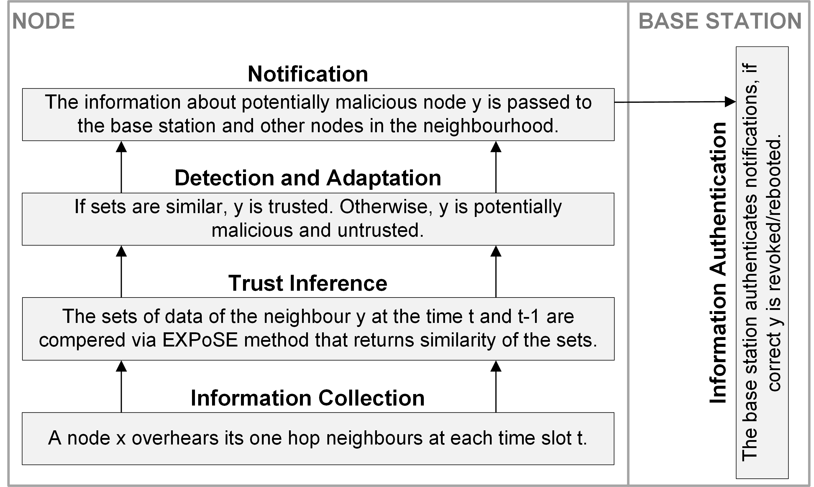
Figure 1. The Antilizer architecture.

5. A Self-Referenced Trust Model to Detect Potentially Malicious Nodes

This section describes the Antilizer trust model in detail. First, we give an explanation of the network metrics used for neighbourhood surveillance and our method of collecting information through overhearing. Then, we present in detail how we use the network metrics with the EXPoSE method to infer trust.

5.1. Neighbourhood Surveillance with Network Overhearing

WSN nodes make communication decisions regarding collaboration with a neighbour node without taking into account that the neighbour might become malicious and violate the underlying protocol rules. For example, a malicious neighbour can alter data or falsify shared information. To address this problem, we introduce trustworthiness as an additional metric to be used by a node when making these decisions.

Network Overhearing. Nodes collect network behaviour information for all of their one-hop neighbours. Information collection is done by overhearing radio packet transmissions in their reception range even if they are not intended recipients (Paris et al., 2013). The use of overheard information does not guarantee the capture of all one-hop neighbour information. Fig. 2 illustrates where node B can overhear packets sent from D to E; however, it cannot hear any packets that E might have received from G. Additionally, leaf nodes such as G, do not perform any forwarding tasks; thus not all of their metric can be measured. Despite these limitations, the information collected using network overhearing is sufficient to describe nodes’ behaviour and infer their trust values.

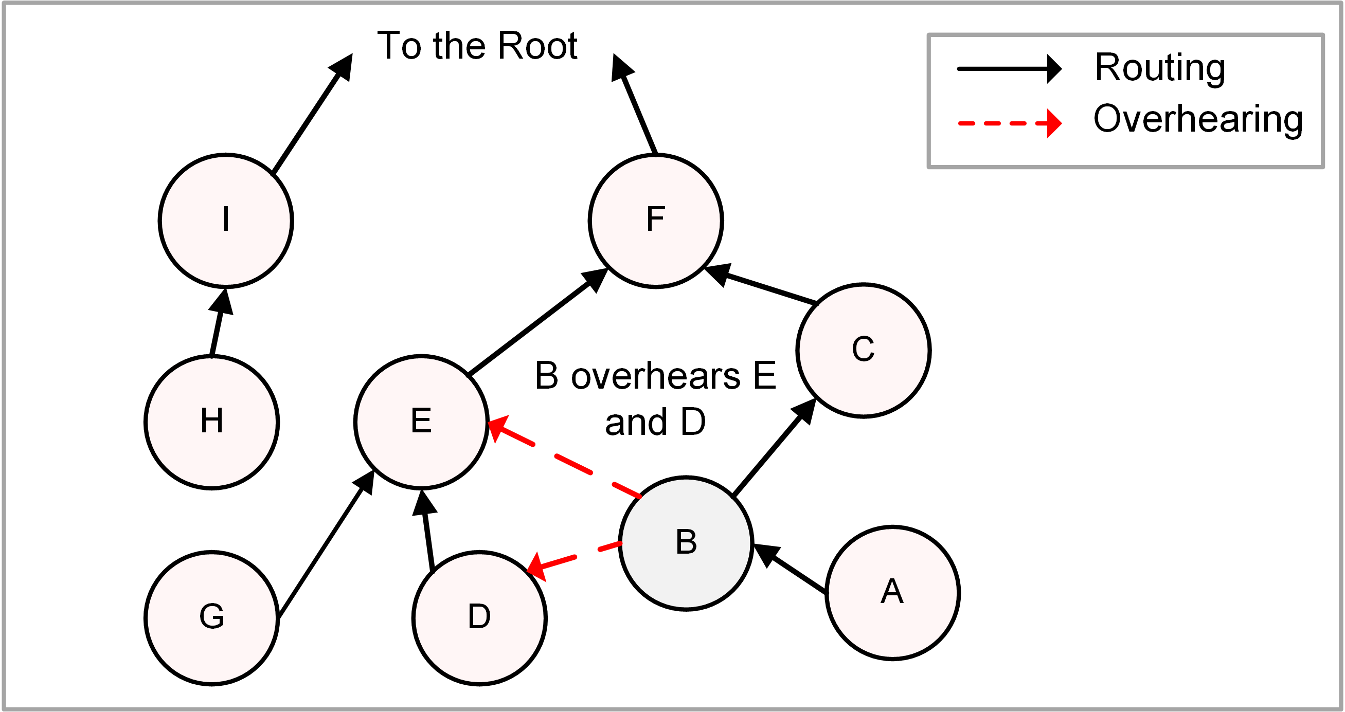
Figure 2. The overhearing phenomenon.

Network Metrics. The use of overhearing overcomes the problem of using potentially dishonest information. Node $x$ trusts only itself and the information that it can overhear without using the content of the communication. This information is stored as a set of network metrics. Table 1 lists the metrics collected by node $x$ for each of its one-hop neighbours $y\in\mathcal{N}_{x}(t)$ within a given time slot. These are added to a network metric vector $\mathbf{v}_{x,y}(t)\in\mathbb{R}^{d}$ at every time slot $t$, where $d=3$ is the number of metrics.

Table 1. Network metrics retrieved via overhearing

Metrics	Description
Tx	the number of packets the node $y$ transmitted to its neighbours
Rx/Tx	the ratio of the number of received and the number of transmitted packets at node $y$ (forwarding indication)
Rank	the average rank of the node $y$

5.2. Temporal Similarity of Network Metrics

The network metrics collected via overhearing change over time. They do not follow a specific distribution. The use of a parametric solution, such as a Gaussian distribution, reduces the reliability of the results obtained. Instead of assuming a certain distribution, we exploit a state-of-the-art non-parametric technique called the Expected Similarity Estimation method (EXPoSE) (Schneider et al., 2016). We choose ExPoSE because of its proven accuracy and its ability to be altered to work on low-power devices such as sensor nodes. We use EXPoSE with a set of approximations to reduce its storage requirements. Without these approximations EXPoSe would be unusable on resource-restricted sensor nodes.

Network Metrics Similarity. In the EXPoSE method, the network metrics are combined into a vector $\mathbf{v}_{x,y}(t)$ for each time slot $t$. The vectors are then mapped into Hilbert space $\mathcal{H}$. The mapping is done using the function $\phi$ at every time slot $t$. The change between two consecutive vectors is described through the expected similarity measure defined below.

Definition 1 (Expected similarity).

Given a node $x$ and $y\in\mathcal{N}_{x}(t)$, the expected similarity between the vector $\mathbf{v}_{x,y}(t)$ at time $t$ and its previous version at time $(t-i)$, $\mathbf{v}_{x,y}(t-i)$, for $i=1,2,...,n$ with $n$ being the number of past vectors, is defined as

(1) $$\eta(\mathbf{v}_{x,y}(t)) = \sum_{i=1}^{n}k(\mathbf{v}_{x,y}(t),\mathbf{v}_{x,y}(t-i))$$

$$= \sum_{i=1}^{n}\langle\phi(\mathbf{v}_{x,y}(t)),\phi(\mathbf{v}_{x,y}(t-i))\rangle.$$

The kernel function $k(\cdot,\cdot)$ computes the inner product of two vectors in $\mathbb{R}^{d}$ after mapping them into higher dimensional Hilbert space $\mathcal{H}\in\mathbf{R}^{d^{\prime}}(d^{\prime}\geq d$) through a mapping function $\phi(\cdot)$. The term $\langle\cdot,\cdot\rangle$ denotes the inner product of the two vectors. For more information regarding the definition of the kernel function, we refer readers to (Hsu et al., 2003).

Although the kernel function $k(\cdot,\cdot)$ allows the computation of the inner product without ’visiting’ the high dimensional Hilbert space $\mathcal{H}$, it does not support the computation of the inner product in an incremental manner. The computation of the inner product in a incremental way is important to the implementation of this method on resource-constrained sensor nodes. Incremental updates allow the accurate capture of the data stream dynamics of $\mathbf{v}_{x,y}(t)$ in way that requires minimal computation and storage. This is achieved because $\eta(\mathbf{v}_{x,y}(t))$ does not have to be recomputed at every time slot $t$. We realise incremental updates through the use of a kernel approximation (KEA) vector which we defined below.

KEA Vector. By using the KEA vector, $\mathbf{$\mathrm{\SIUnitSymbolMicro}\text{/}$}_{x,y}(t)$, Eq. (1) becomes:

(2) $$\eta(\mathbf{v}_{x,y}(t)) = \langle\phi(\mathbf{v}_{x,y}(t)),\frac{1}{n}\sum_{i=1}^{n}\phi(\mathbf{v}_{x,y}(t-i))\rangle$$

$$= \langle\phi(\mathbf{v}_{x,y}(t)),\mathbf{$\frac{\mathrm{\SIUnitSymbolMicro}}{}$}_{x,y}(t)\rangle$$

where $\mathbf{$\mathrm{\SIUnitSymbolMicro}\text{/}$}_{x,y}(t)$ can be updated in an incremental manner as:

(3) $${$\frac{\mathrm{\SIUnitSymbolMicro}}{}$}_{x,y}(t)=\gamma\phi(\mathbf{v}_{x,y}(t-1))+(1-\gamma){$\frac{\mathrm{\SIUnitSymbolMicro}}{}$}_{x,y}(t-1).$$

The term $\gamma\in[0,1]$ denotes an automatic decay factor that controls the speed at which the trust metric will change to the occurrence of new information. A larger $\gamma$ results in the faster decay of past information.

The KEA vector ${$\mathrm{\SIUnitSymbolMicro}\text{/}$}_{x,y}(t)$ is computed using the overheard network metrics collected in previous time slots, $\mathbf{v}_{x,y}(t^{\prime})$, where $t^{\prime}<t$. The metrics used for the update of ${$\mathrm{\SIUnitSymbolMicro}\text{/}$}_{x,y}(t)$ need to come from a trusted, non-malicious node. The network metrics generated from potentially malicious nodes are detectable when they first occur because the difference between the current and past metrics will be large. As time continues $\mathbf{$\mathrm{\SIUnitSymbolMicro}\text{/}$}_{x,y}(t)$ will change to incorporate the new network metrics.

To prevent the adaptation of $\mathbf{$\mathrm{\SIUnitSymbolMicro}\text{/}$}_{x,y}(t)$ to a malicious node we define a parameter $\alpha$ to determine which overheard network metrics get included in the KEA vector. When $\eta(\mathbf{v}_{x,y}(t))>\alpha$ the network metrics for that time slot $t$ will not be used to update the KEA vector, (i.e. ${$\mathrm{\SIUnitSymbolMicro}\text{/}$}_{x,y}(t)={$\mathrm{\SIUnitSymbolMicro}\text{/}$}_{x,y}(t-1)$), as the new behaviour is likely to be malicious. According to our extensive simulations in Sec. 9.3, $\alpha\in[0.7,0.9]$ ensures the detection of more than $98.6$% anomalies with low rate of false positives ($\sim 3.6$%) (see Fig. 10).

Mapping Function Approximation. We use the radial basis function (RBF) (Hsu et al., 2003) as the kernel function to compute KEA. RBF has been widely used in many machine learning applications, including non-parametric regression, clustering and neural networks. We can not directly use RBF because it transforms data vectors into an infinite dimensional space (i.e. $\phi(\mathbf{v}_{x,y}(t))\in\mathbb{R}^{\infty}$ and $\mathbf{$\mathrm{\SIUnitSymbolMicro}\text{/}$}_{x,y}(t)\in\mathbb{R}^{\infty}$) whose storage would exceed that of a sensor node. We fix this problem with the use of a Monte Carlo approximation of the RBF mapping function. An inverse Fourier transform is used to approximate the Gaussian RBF kernel (Rahimi and Recht, 2008). The approximation function $\hat{\phi}(\mathbf{v})$ is given by the Euler equation:

(4) $$\hat{\phi}(\mathbf{v}_{x,y}(t))=\frac{1}{\sqrt{m}}exp(i\mathbf{Z\mathbf{v}_{x,y}(t)})$$

where $i$ denotes the imaginary unit ($i^{2}=-1$), $\mathbf{Z}$ is a $m\times d$ matrix where each element $\mathbf{Z_{i,j}}\sim\mathcal{N}(0,1/\sigma^{2})$, and $m$ represents the number of Monte Carlo samples. The operation in Eq. 4 is depicted in Fig. 3. The Euler equation results in $2m$ elements where the odd elements store the real parts and the even elements store the imaginary parts of the complex number.

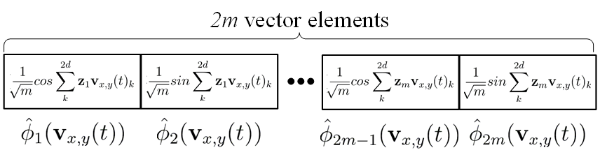
Figure 3. Approximation of the mapping function $\hat{\phi}(\mathbf{v}_{x,y}(t))$ results in $2m$ elements.

The expected similarity $\eta(\mathbf{v}_{x,y}(t))$ in Eq. 2 then becomes:

(5) $$\eta(\mathbf{v}_{x,y}(t))\approx\langle\hat{\phi}(\mathbf{v}_{x,y}(t)),\frac{1}{n}\sum_{i=1}^{n}\hat{\phi}(\mathbf{v}_{x,y}(t-i))\rangle$$

where $1/n\sum_{i=1}^{n}\hat{\phi}(\mathbf{v}_{x,y}(t-i))$ is computed in an incremental manner with Eq. (3).

The expected similarity computation method which uses Monte Carlo approximation is given in Alg. 1. The computational complexity of Alg. 1 reduces from $O(mnd)$ to $O(m\log d)$ for all $t$, where $m$ denotes the number of Monte Carlo samples, $n$ denotes the number of past vectors, and $d$ denotes the number of network metrics obtained at every time $t$ (Schneider et al., 2016). This reduction in complexity is a result of $\phi(\mathbf{v}_{x,y}(\cdot))$ not having to be recomputed in each time slot. Note that, $\eta(\mathbf{v}_{x,y}(t))\in[0,1]$ is normalized by the $1/\sqrt{m}$ in Eq. (4).

Input :  $\mathbf{v}_{x,y}(t)$: the network metrics of $y$ observed from $x$ at time $t$

$\mathbf{$\mathrm{\SIUnitSymbolMicro}\text{/}$}_{x,y}(t)$: the KEA vector of $y$ observed from $x$ at time $t$

$\sigma^{2}$: the standard deviation for Monte Carlo sampling

$\mathbf{z}$: the vector of $m$ Gaussian samples from $\mathcal{Z}~{}(0,1/\sigma^{2})$

$\alpha$, $\gamma$: the parameters to control KEA vector adaptation

Output : $\eta(\mathbf{v}_{x,y}(t))$: the expected similarity of the network metrics of $y$ observed from $x$ at time $t$

1 $\hat{\phi}(\mathbf{v}_{x,y}(t))\leftarrow 0,\mathbf{$\mathrm{\SIUnitSymbolMicro}\text{/}$}_{x,y}(1)\leftarrow\hat{\phi}(\mathbf{v}_{x,y}(1)),\eta(\mathbf{v}_{x,y}(t))\leftarrow 0$

2 /* STEP 1: mapping function approximation */

3 for $j\Leftarrow 1,2...,m$ do

4       $\hat{\phi}_{j}(\mathbf{v}_{x,y}(t))\leftarrow\frac{1}{\sqrt[]{m}}exp(i\mathbf{z}\cdot\mathbf{v}_{x,y}(t))$

5      

6 end for

7/* STEP 2: compute expected similarity */

8 $\eta(\mathbf{v}_{x,y}(t))\leftarrow\langle\phi(\mathbf{v}_{x,y}(t)),\mathbf{$\mathrm{\SIUnitSymbolMicro}\text{/}$}_{x,y}(t)\rangle$

9 /* STEP 3: update KEA vector for time $t+1$ */

10 if $k>1$ and $\eta(\mathbf{v}_{x,y}(t))<\alpha$ then

11       ${$\mathrm{\SIUnitSymbolMicro}\text{/}$}_{x,y}(t)=\gamma\phi(\mathbf{v}_{x,y}(t-1))+(1-\gamma){$\mathrm{\SIUnitSymbolMicro}\text{/}$}_{x,y}(t-1)$

12 end if

return $\eta(\mathbf{v}_{x,y}(t))$

Algorithm 1 Expected similarity $\eta(\mathbf{v}_{x,y}(t))$ computation

In the next section we show how the similarity measure is mapped to a trust value and used to enhance the objective function of the routing algorithm.

6. Application of the Self-Referenced Trust Model to Data Routing

In this section we describe how the trust, computed from the similarity measure of network metrics, is used in the routing algorithm to affect routing decisions. The routing is an example of node collaboration where communication decisions can be based on the notion of trust. First, we discuss the class of routing protocols that can benefit from our scheme. Then, we show how our trust metric can be used by a routing algorithm objective function to avoid areas affected by a network level attack.

6.1. Distance Vector Routing Protocols: RPL as an Example

Antilizer can be applied to any distance-vector routing protocol where a distance measure (e.g. hop count, or respective link qualities) is used to determine the best packet forwarding route. In this paper we use RPL (Routing Protocol for Low-Power and Lossy Networks) (Brandt et al., 2012). RPL is a standardized IPv6-based multi-hop routing solution widely used in WSNs. It is an appropriate protocol for the evaluation of Antilizer because it requires an objective function where the trustworthiness can be added as an additional metric. It is important to mention that Antilizer affects only the objective function; therefore, it can be easily applied to any other routing protocol based on a distance-based objective function.

An objective function defines how a node translate one or more network metrics and constraints into a $\rm Rank$ value. $\rm Rank$ is used to determine the best neighbour to forward data to the base station. The $\rm Rank$ between the node $x$ and its neighbours $y\in\mathcal{N}_{x}(t)$ is given by

(6) $$\rm Rank_{x}(t)=\left\{\begin{array}[]{l l}\underset{y\in\mathcal{N}_{x}(t)}{\min}(p_{x,y}(t)+\rm Rank_{y}(t))&\quad x\notin\mathcal{R}\vspace{0.2em}\\ {\rm RootRank}_{x}&\quad x\in\mathcal{R}\end{array}\right.$$

where $p_{x,y}(t)>0$ denotes the penalty of using the link $(x,y)$ at time slot $t$, and ${\rm RootRank}_{x}\geq 0$ is the smallest $\rm Rank$ value in the routing tree. The smallest $\rm Rank$ value in a correctly operating network belongs to the root $x$.

The $mrhof$ objective function is used in the Contiki implementation of RPL. It defines $p_{x,y}(t)$ as a moving average function that uses the expected number of transmissions (ETX) as the routing measure (Contiki operating system, page):

(7) $$p_{x,y}(t)=\textsf{ALPHA}p_{x,y}(t-1)+(1-\textsf{ALPHA})\textsf{ETX}_{x,y}(t)$$

where $\textsf{ALPHA}=\{0.15,0.3\}$. In our work we add the trustworthiness of individual nodes to the routing measure. This enhanced objective function is given next.

6.2. Trust-based RPL Objective Function

The expected similarity $\eta(\mathbf{v}_{x,y}(t))$ of the network metric vector $\mathbf{v}_{x,y}(t)$ at time $t$ is included in the $\rm Rank$ computation in Eq. (6) through the link penalty function in Eq. (7). It is included as subjective ’penalty’, or weighting function, called the Subjective Trust.

Definition 2 (Subjective Trust).

Given a node $x$ and its one-hop neighbour $y\in\mathcal{N}_{x}(t)$, the subjective trust $\tau_{x,y}(t)$ is the penalty that $x$ gives to $y$ at time $t$. Its value is defined through the hyperbolic function:

(8) $$\tau_{x,y}(t)=-csch(k\eta(\mathbf{v}_{x,y}(t))-k)+csch(-k)+1$$

where $csch(\cdot)$ denotes the hyperbolic cosecant function, and $k$ is a parameter used to control the detection sensitivity of our solution.

This function provides the continuous transient where $\tau_{x,y}(t)\approx 1$ for all $\eta(\mathbf{v}_{x,y}(t))\leq\alpha$. For $\eta(\mathbf{v}_{x,y}(t))>\alpha$, the value of $\tau_{x,y}(t)$ grows exponentially. By adjusting $\alpha$ and $k$, the sensitivity of the scheme can be controlled. Fig. 4 illustrates the hyperbolic function where $\alpha=0.75$ and $k=6$. Function $f(x)$ takes as an input the expected similarity $\eta(\mathbf{v}_{x,y}(t))$ obtained in Alg. 1 and it returns the subjective trust $\tau_{x,y}(t)$.

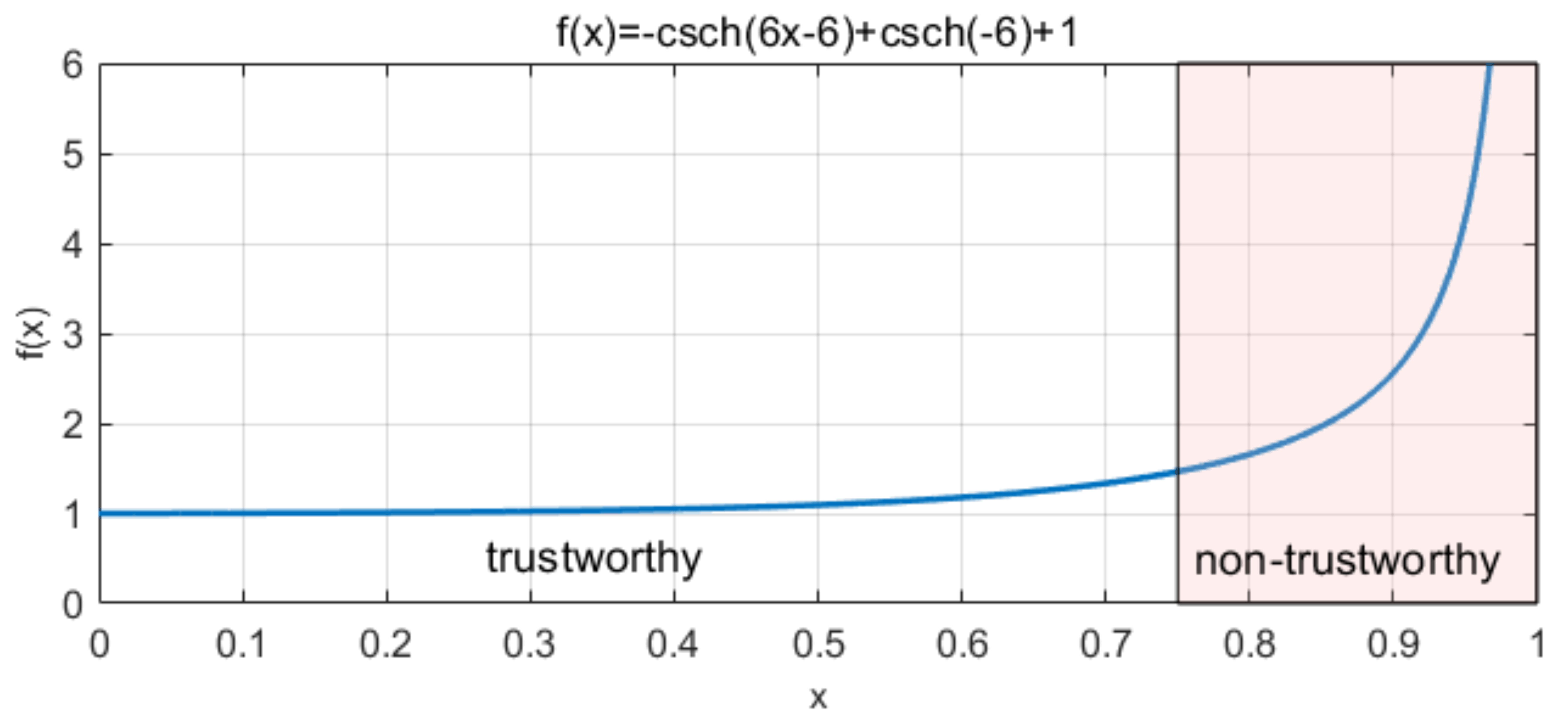
Figure 4. Hyperbolic cosecant function with $k=6$.

As can be observed from Def. 2, $\tau_{x,y}(t)$ is bounded between $1$ and $\infty$, i.e. $\tau_{x,y}(t)\in[1,\infty]$. $\tau_{x,y}(t)=1$ indicates that node $y$ is $100$% trustworthy from the perspective of node $x$. Large values of $\tau_{x,y}(t)$ indicate the reduction of trustworthiness towards the node $y$. This measure of the trustworthiness of individual nodes is then used as a weighting function in the link penalty function $p_{x,y}(t)$ in Eq. (7):

(9) $$\small\hat{p}_{x,y}(t)=\textsf{ALPHA}\hat{p}_{x,y}(t-1)+(1-\textsf{ALPHA})\tau_{x,y}(t)\textsf{ETX}_{x,y}(t).$$

The addition of trustworthiness directly affects a nodes routing decisions and ensures that it avoids malicious nodes so that the flow of data is not obstructed during an attack.

Remark 1 (Zero performance penalty in no attack scenario).

The hyperbolic function illustrated in Fig. 4 ensures a high penalty when potentially malicious behaviour is detected. It also guarantees optimal performance (i.e. as when default objective function of RPL is used) in no attack scenario, that is, $\hat{p}_{x,y}(t)\approx p_{x,y}(t)$.

Next, we present an agent-based notification scheme to address the limitations of the proposed trust-based scheme.

7. Mobile agent-based notification scheme to stop the disruption of the network

While the self-referenced trust model proposed in Sec. 5 is able to detect potentially malicious change and adapt node’s communication decisions such that the affected area is avoided, it has its own limitations. The scheme can not completely prevent the disruption to the network because the network will eventually require reconfiguration to handle the malicious node, and the adaptation of one node may be interpreted as malicious behaviour by another. To address these issues, we present a notification scheme that uses mobile agents called ANTs (Antilizer Notification ticket) to inform the base station of suspected malicious behaviour, to bound the damage of the attack to a specific area, and prevent the spread of distrust in the network.

First, we introduce the features of ANTs and their working principle. We show how these are applied to the routing example. Finally, we discuss how the information carried by ANTs can be authenticated at the base station.

7.1. Overview of the ANT and ANT’s Features

When node $x$ detects a change in network behaviour of its parent $y$, it reduces its trustworthiness. In the example of routing this leads to $x$ changing the routing path (i.e. $x$ chooses a node with the lowest rank in the neighbourhood). At the same time, $x$ creates an ANT which does the following:

1. It migrates from the node $x$ to its new parent $y^{\prime}$ while carrying the ID of the potentially malicious node (i.e. $x$’s old parent $y$).

2. After it successfully migrates to $y^{\prime}$, it triggers a broadcast message to all one-hop neighbours of $y^{\prime}$, $\mathcal{N}_{y^{\prime}}(t)$, to notify them of potential malicious activity in the neighbourhood, and to prevent the spread of distrust caused by network variations.

3. The ANT then moves to the next hop along the established route and repeats this process until it reaches the base-station.

4. The ANT delivers the ID of the potentially malicious node to the base-station which decides if node $y$ should be revoked/reprogrammed (may involve human interaction).

Next, we further discuss the features of this notification scheme, as well as the introduced overhead.

Protection at Low Overheads. As described before, an ANT does two operations: it travels to the base-station along the RPL tree, and it broadcasts a one-hop message at each hop in the route. Given a node which has a route to the base station of $z$-hops, the number of extra messages introduced by each ANT is $2z+1$. ANT messages require no more than one data packet of less than $160$ bytes. Therefore, the operations done by ANTs are very lightweight and with low operational overhead as shown in Sec. 9.3 (less than $1$%).

Guarantees for No Attack Scenarios. ANTs will be created only by nodes that detect a change in network behaviour of their parent. No ANT will be spawned when no attacks occur, and no extra communication is required. Our experimental results in Sec. 9.3 show that the percentage of false positive detections is less then 3.4% for $\alpha\in[0.7,0.9]$, and there is a zero performance penalty when Antilizer is run no attack scenario.

Distinguishes Genuine Change from Malicious Behaviour. When node $x$ detects a malicious behaviour in $y$ it changes to an alternative route through $y^{\prime}$ (which has the lowest rank in the neighbourhood) and sends its ANT towards the base station (see Fig. 5). This change increases the traffic of $y^{\prime}$. From the perspective of its neighbours $n_{1}$ and $n_{2}$, $y^{\prime}$ is likely to be seen as malicious due to its increasing $\rm T_{x}$ and $\rm R_{x}$. As a result, node $y^{\prime}$ is penalized by this false positive detection, and $n_{1}$ and $n_{2}$ switch their routes to $n_{3}$, which further spreads distrust. If this spread is left unchecked, nodes will run out of ’safe’ routes and RPL will be unable to converge to a stable routing tree.

In our scheme, an ANT created by $x$ triggers a broadcast message at its new RPL-tree parent $y^{\prime}\in\mathcal{N}_{x}(t)$. The ANT informs all of the one-hop neighbours of $\mathcal{N}_{y^{\prime}}(t)$ (e.g. nodes $n_{1}$ and $n_{2}$) of the change at $x$. Now instead of flagging $y^{\prime}$ as potentially malicious, nodes allow a certain period of time (a refractory period) to adapt to the new network behaviour caused by the change of routes of $x$. ANTs reduce the number of false positive detections which improves Antilizer performance and bounds the damage of an attack to a specific area.

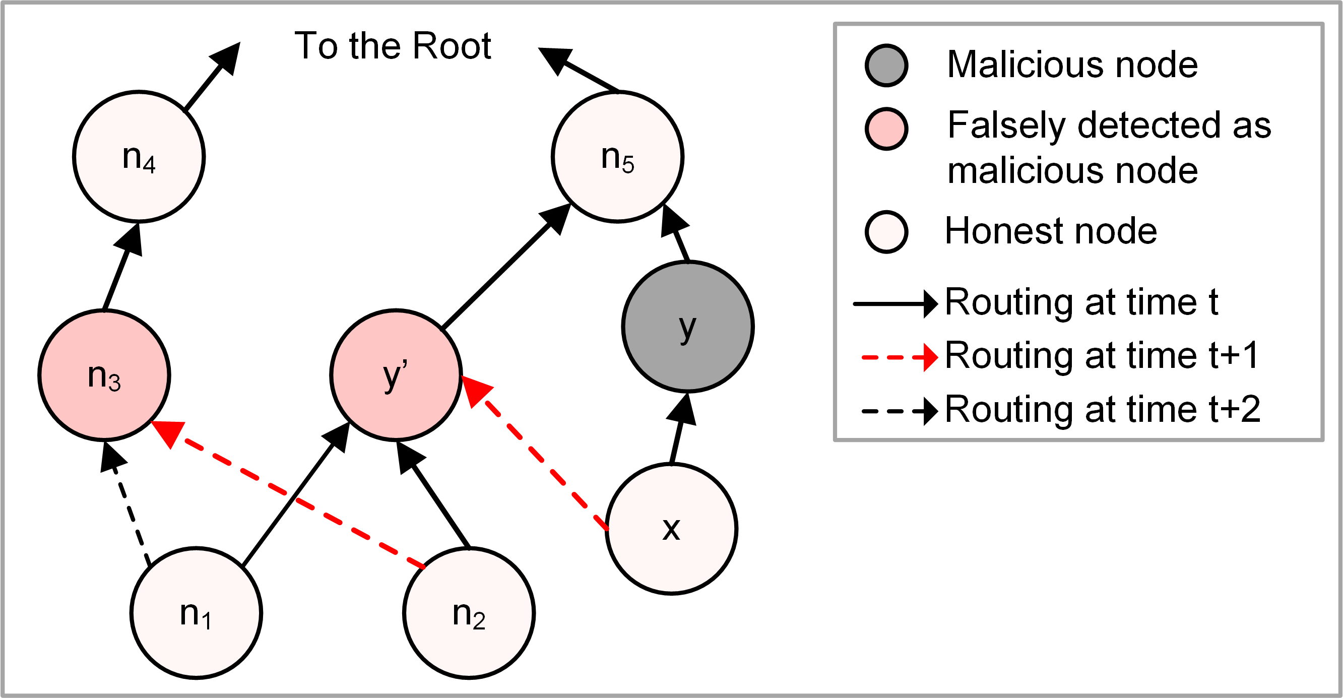
Figure 5. An illustration of a attacker’s neighbourhood (node $y$ is the attacker that has been chosen by node $x$ as its parent, $x$ and $n_{1}$-$n_{5}$ are honest nodes).

To validate the authenticity of the information provided by ANTs at the base station, we use a filtering mechanism described next.

7.2. Credibility of Information carried by ANTs

Here we discuss the potential drawbacks of our notification scheme and scenarios when it can be compromised.

Filtering mechanism to authenticate information. An attacker can use ANTs to flood a network. The attacker can create a number of ’falsified’ ANTs by switching between its parents. The base-station would quickly be able to identify this as malicious activity as ANTs would arrive at high frequency from a single source. The flooding of ANTs would also not prevent a node from routing away from a malicious neighbour. The filtering mechanism at the base station that is run for individual time slot is presented in Alg. 2. Parameters $\theta_{b}$ and $\theta_{n}$ are user defined, depending on the requirements on mechanism sensitivity.

Input :  $\rm ANT(a_{1},a_{2})$: The ANT that carries the ID of the blacklisted node ($a_{1}$) and the ID of node that reported blacklisting ($a_{2}$)

$\rm ANT_{\text{data}}\in\mathrm{R}^{ixj}$: A matrix which individual entries indicate how many times nodes $\{1,\ldots,i\}$ have been blacklisted by nodes $\{1,\ldots,j\}$ where $i,j\in{\mathcal{S}}$

$\theta_{b},\theta_{n}$: Parameters that control the filtering mechanism

$n$: A number of $\rm ANT(a_{1},a_{2})$ that arrived within time slot

Output : $c\in\{\textsf{GD},\textsf{CA},\textsf{FP}\}$

1 $\rm ANT\leftarrow\mathbf{0}$

2 for $l\Leftarrow 1\cdots n$ do

3       $\rm ANT(a_{1},a_{2})\leftarrow\rm ANT_{(}a_{1},a_{2})+1$

4      

5 end for

6for $k\Leftarrow 1\cdots i$ do

7       if $|\rm ANT(i,k)|>\theta_{b}$ /*where $|\rm ANT(i,k)|$ indicates the number of non-zero elements of vector*/ then

8             $c\leftarrow\textsf{GA}$ /*Genuine attack, $i$ is malicious*/

9            

10       end if

11      else if $|\rm ANT(i,k)|<\theta_{b}$ and $\rm max(\rm ANT(i,k))\geq\theta_{n}$ then

12             $c\leftarrow\textsf{CA}$ /*Compromised ANT by $k$ for which $\rm ANT(i,k)$ is max*/

13            

14       end if

15      else

16             $c\leftarrow\textsf{FP}$ /*False positive*/

17            

18       end if

19      

20 end for

return $c$

Algorithm 2 Filtering mechanism to authenticate information

Encryption to avoid information alteration. Our attacker model does not assume the alteration of packet’s content. To mitigate these sorts of attacks there is the need of encrypting the content of ANT messages. This is a natural extension of this work. Encryption alone is usually not sufficient as an attacker could fetch encrypted packets and replay them. Once again, using the filtering mechanism the base station would detect a large number of ANTs being send from a single node and would be able to identify malicious behaviour.

Blacklisting to ensure avoidance. Lastly, we discuss the cost of losing some ANTs. As Antilizer ensures routing around the affected areas, nodes will never re-establish routes through potentially malicious nodes until these are re-approved by the base station. If the base station does not receive any ANT reporting malicious activity, the area affected by that node will still be avoided.

8. Implementation

We implemented Antilizer in Contiki (Contiki operating system, page) version 3.1, an open source operating system for WSNs and IoT. Contiki provides an IPv6 stack (uIPv6) and the RPL routing protocol. Our implementation used both. In this section, we describe key aspects of our implementation.

Mac and IPv6. For the MAC layer, a CSMA/CA driver was used with default settings in Contiki. The neighbour table size is set to 50. The radio duty cycling is disabled during all our experiments. The maximum transmission attempts to re-send a packet is 5. In regards to the IPv6 stack, the packet reassembly service is disabled. The UIP_CONF_IGNORE_TTL is set to zero to ignore the TTL flag in the packet headers. The HC6 SICSlowpan header compression is used.. The application layer generates UDP packets at a fixed rate of one every four seconds. The size of a data packet is 160 bytes (8 bytes for payload and the rest is used for IPv6 header).

Attacks. Each compromised node $x_{c}\in\mathcal{N}$ is able to initiate one or more of the malicious activities described in Sec. 3. We give a specific description of our attack implementation below:

1. Sinkhole attack - The node $x_{c}$ advertises falsified rank information (i.e. it claims that it’s a sink, $\rm Rank_{x_{c}}(t)={\rm RootRank}_{x}$, $x\in\textrm{R}$.

2. Blackhole - A compromised node $x_{c}$ advertises falsified rank information to lure the traffic and then fails to forward any data received from it’s neighbours.

3. Hello Flood - The node $x_{c}$ broadcasts hello packets at a very high rate to all of its one-hop neighbours $y\in\mathcal{N}_{x_{c}(t)}$.

Routing objective function and metrics retrieval. The RPL routing protocol is used with the ETX objective function and default settings. The RPL_MOP_NO_DOWNWARD_ROUTES option is enabled since downward routing is not used in our experiments. DIO_INTERVAL_MIN and DIO_INTERVAL_DOUBLINGS broadcast routing metadata every $512$ to $1024$ms.

To implement overhearing, we extended the Contiki network link stats module. The data is stored in a separate neighbour table used only by Antilizer. The network metrics $\rm T_{x}$ and $\rm R_{x}$ are collected by callbacks in link stats, whereas the public functions are used to retrieve the $\rm Rank$ metric. The minimum $\rm Rank$ with hysteresis objective function (rpl-mrhof.c) is used as the base when no malicious behaviour is detected. The expected similarity value is calculated every $20$ seconds for each node in the neighbour table, and used as a weight for the calculation of that node’s $\rm Rank$.

Notification via ANTs. The ANTs were implemented using RPL ICMP6 messages and RPL broadcast messages. When a node changes it’s next hop neighbour due to a change in rank weight from Antilizer, it produces an ANT. The first hop of the ANT goes from the node to its new upstream next hop and contains the IPv6 ID of the node considered malicious. When the ANT is received by the new upstream node, the receiver sends an IPv6 broadcast to all of it’s one hop neighbours. The ANT eventually arrives at the base station where it is verified, and its data used.

9. Experimental Evaluation

In this section, we present the results of an extensive simulation study to evaluate the performance of Antilizer.

9.1. Experimental Setup

We performed our evaluation by using the Contiki simulator Cooja. As a routing protocol, we use the RPL. We consider networks with $25$, $50$ and $100$ nodes randomly distributed over a $100$m$\times 100$m, $200$m$\times 200$m, $400$m$\times 400$m area, respectively. Each node has a $\rm T_{x}$ range of $50$m and periodically sends out data every 4 seconds with an initial random offset.

To configure Antilizer we set the number of Monte Carlo samples to $m=200$ with the standard deviation set to $\sigma^{2}=0.35$. We use a hyperbolic cosecant function depicted in Fig. 4. The parameter $\alpha$ is set to $0.75$ as explained in Sec. 9.3. The duration of a time slot is set to $20$ seconds.

We consider a set of attack scenarios in the simulations:

1. A single attacker in the network exploiting one of three attacks defined in Sec. 8,

2. A multi-attacker case where the attackers belong to the same category of attacks (i.e. we vary an attack for non-intrusive to an intrusive scenario with $10$% of the nodes being malicious).

Simulations are run for $4$ hours of simulation time with the attack starting time at $20$ minutes for a $25$ nodes simulation or $40$ minutes for a $50$ nodes and $100$ nodes simulation.

9.2. Performance Metrics

The effectiveness of Antilizer is evaluated based on the following metrics:

• End-to-End (E2E) Data Loss - Ratio between the total number of packets successfully received by the base station and the number of packets sent by the nodes.

• Average End-to-End (E2E) Delay - Average time needed for a packet to travel between the source and the base station.

• Overhead - The percentage of additional messages created upon an incident detection compared to the total number of messages sent in the network.

• Detection Reliability - Successful detection rate and the false positive detection rate for various simulation scenarios.

We first evaluate the performance of Antilizer with no attack scenario to show that there is a zero performance penalty. We then evaluate the performance of Antilizer with malicious nodes in the network. Our results show that our system can detect data loss with high reliability and route around affected areas. These changes reduce the loss rate that has been caused by the attacks, as well as the data delivery delay.

9.3. Performance Results

Below, we present the simulation results of our evaluation of Antilizer for varied attack scenarios and topologies.

No Attack Scenario. Figure 6 presents the performance of Antilizer with no attack scenario. We show that there is a zero performance penalty if Antilizer is run in the network with no attacker.

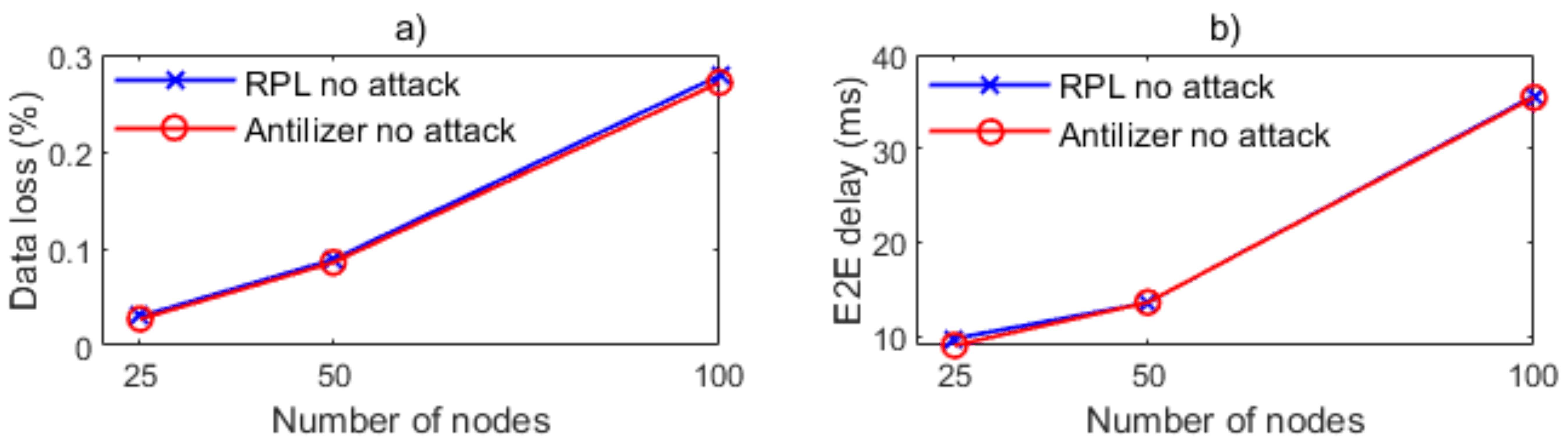
Figure 6. Antilizer performance for no attack scenario in $25$, $50$ and $100$ nodes network: (a) Data loss. (b) E2E delay.

Sinkhole Attack. Antilizer detects a change in the rank and an increase in receptions and transmissions during a sinkhole attack. Once detected, nodes reroute communication whilst triggering the notification scheme. From the Figure 7 we can see that there is no notable impact on E2E data loss; however routes are compromised so that data is delayed. Results show that Antilizer keeps the E2E delay in the presence of sinkhole attack close to normal latency. The overheads are very low.

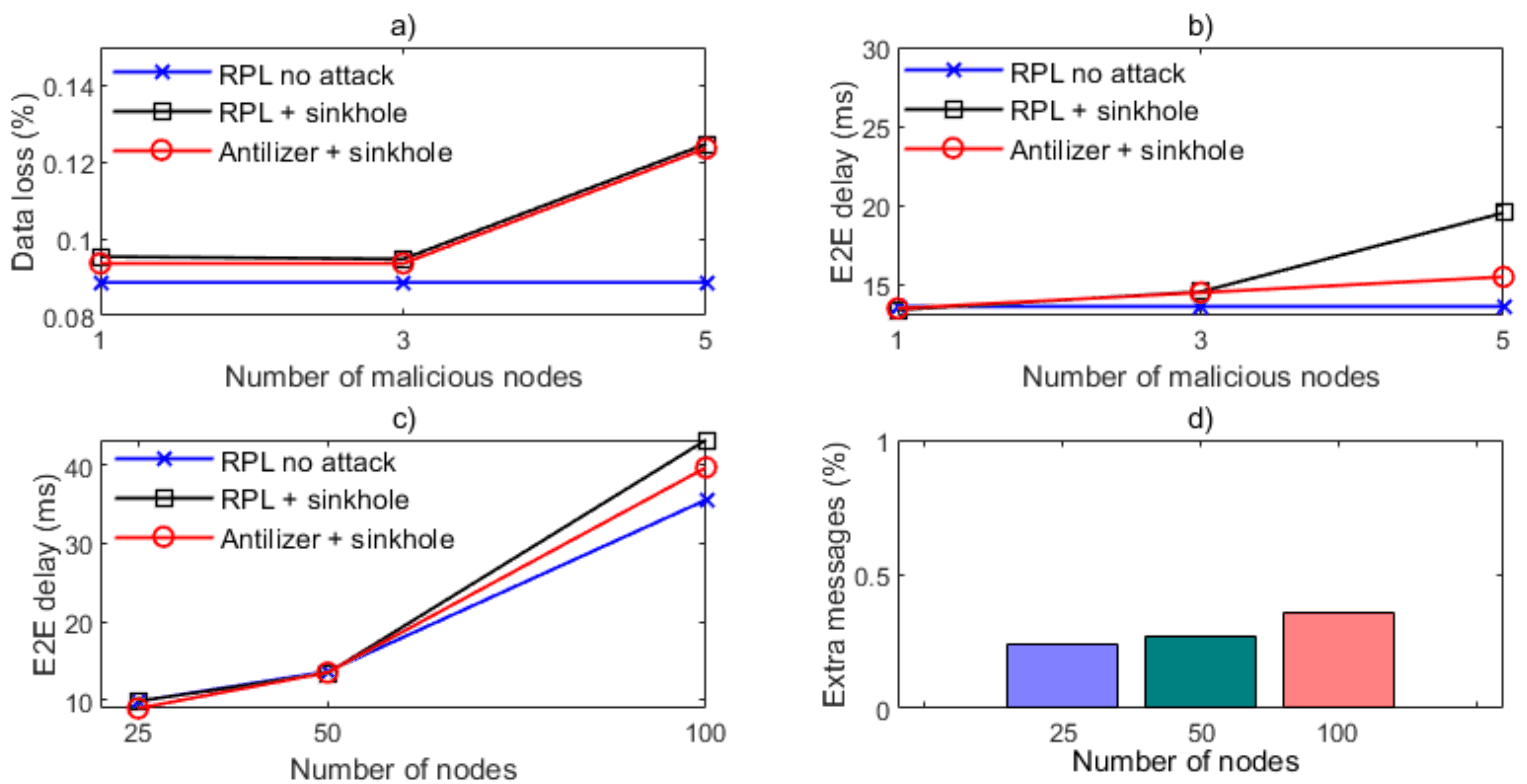
Figure 7. Antilizer performance for sinkhole attack: (a) - (b) Data loss and E2E delay ($50$ nodes, multiple attackers) c) - d) Data loss and Overhead ($25$, $50$ and $100$ nodes, single attacker).

Blackhole Attack. During a blackhole attack, Antilizer detects the drop in transmissions and nodes reroute data whilst triggering the notification scheme. Figure 8 shows that Antilizer reduces the data loss down to 1%, but also it keeps the transmission delay closer to normal latency. The overhead introduced is less then 0.5% across varied attack intensities.

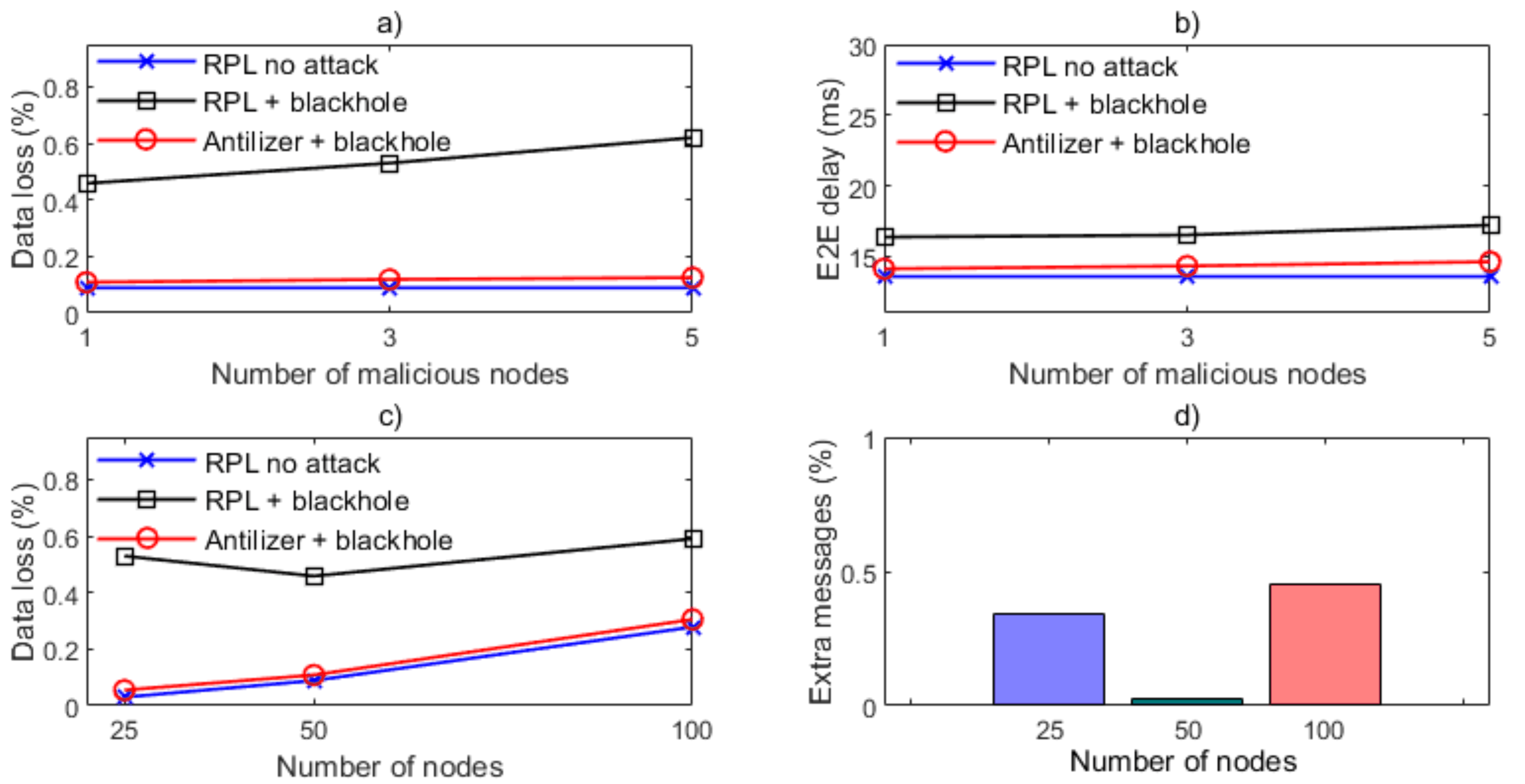
Figure 8. Antilizer performance for blackhole attack: (a) - (b) Data loss and E2E delay ($50$ nodes, multiple attackers) c) - d) Data loss and Overhead ($25$, $50$ and $100$ nodes, single attacker).

Hello Flood Attack. Nodes detect an increase in the transmissions of an attacker. The attack drastically increases the overall number of packets in the network. The transmission delays increase accordingly as can be seen in Fig. 9. Due to the nature of the attack, it is not possible to reroute around the affected regions completely as additional packets are spread across the whole network. However, all nodes are able to detect the attack and send ANTs to the base station. The average time needed for a node to detect and report a hello attacker to the base station is up to two time slots ($40$ seconds). Therefore, its effects could be prevented by the base station in a very short period.

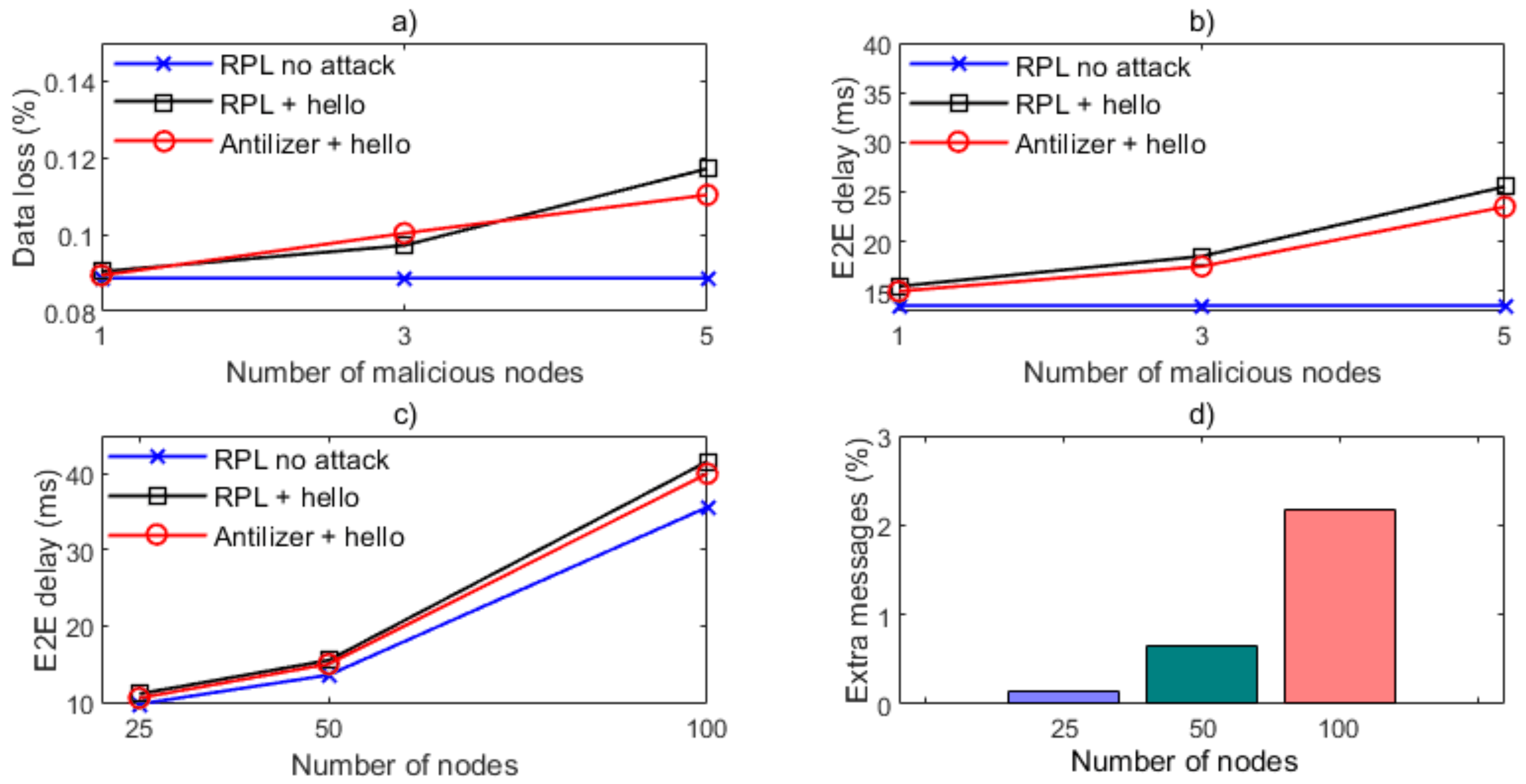
Figure 9. Antilizer performance for hello attack: (a) - (b) Data loss and E2E delay ($50$ nodes, multiple attackers) c) - d) Data loss and Overhead ($25$, $50$ and $100$ nodes, single attacker).

Detection Reliability. The reliability of our detection scheme and its dependence on the choice of parameter $\alpha$ is shown in Fig. 10. We performed extensive simulations of three attacks with a single attacking node in a network of $50$ nodes. Detection rates were calculated as average rates per node. The results show that on average for $\alpha\in[0.7,0.9]$ Antilizer can identify more that 98.6% anomalies with only around 3.6% false positive detections. While $\alpha=0.9$ gives the lowest number of false positives, we opted for more conservative approach and $\alpha=0.75$ which ensures a good sensitivity to all attacks with $99.3$% detection reliability.

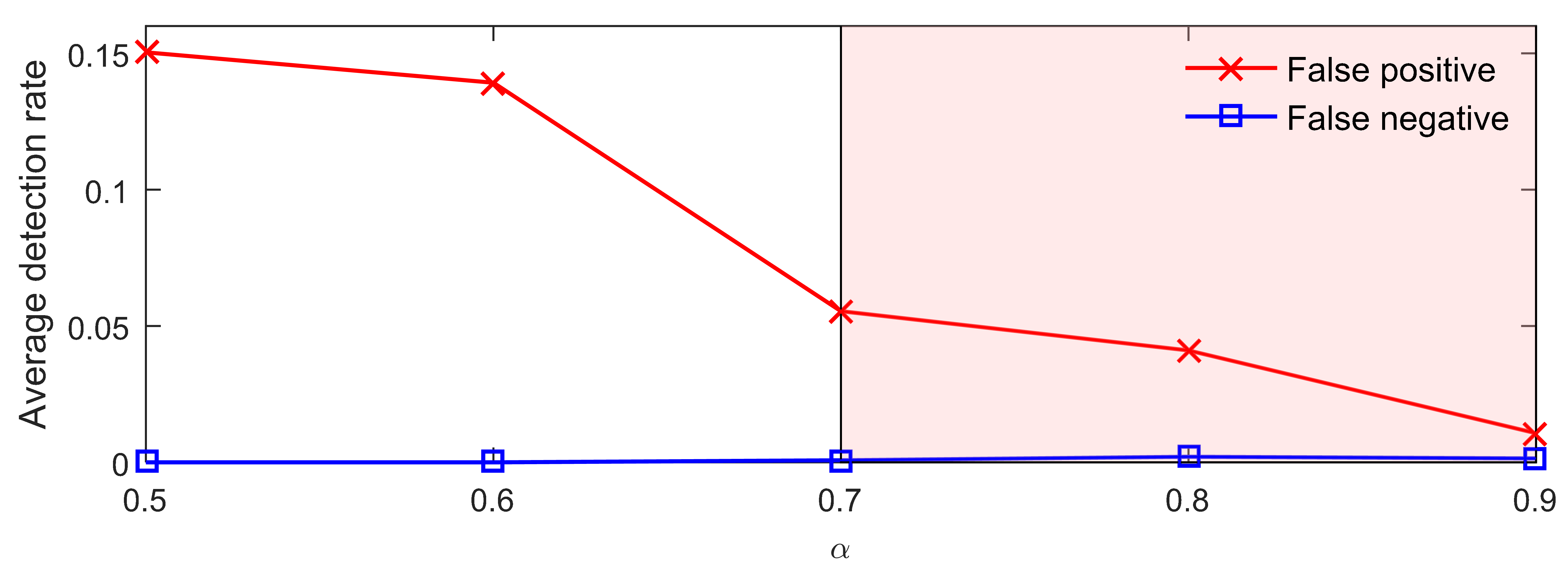
Figure 10. Antilizer detection reliability for $\alpha\in[0.5,0.9]$ in $50$ nodes network (average of four attacks, a single attacker).

10. Conclusions

In this paper, we presented Antilizer, a novel self-healing scheme to defend against attacks aimed at network communications. Upon detecting malicious activities, the system allows data to flow around affected regions so that the network functionality is not compromised. Our experimental results showed high effectiveness in terms of data loss rate requiring low operational overheads for varied attack scenarios.

As part of our future work, we plan to test Antilizer in real test-bed experiments. Also, we plan to improve the attack diagnosis component by exploiting reinforcement-learning schemes. This would support the decision making process at the base station and further improve Antilizer performance.

References

- (1)
- Banerjee et al. (2005) S. Banerjee, C. Grosan, and A. Abraham. 2005. IDEAS: intrusion detection based on emotional ants for sensors. 5th Int. Conf. on Intell.t Sys. Design and Appl. (2005), 344–349.
- Bao et al. (2012) F. Bao, I. R. Chen, M. Chang, and J. H. Cho. 2012. Hierarchical trust management for wireless sensor networks and its applications to trust-based routing and intrusion detection. IEEE Tran. on Netw. and Serv. Manag. 9, 2 (2012), 169–183.
- Brandt et al. (2012) A. Brandt et al. 2012. RPL: IPv6 Routing Protocol for Low-Power and Lossy Networks. RFC 6550. https://doi.org/10.17487/rfc6550
- Chen et al. (2011) D. Chen, G. Chang, D. Sun, J. Li, J. Jia, and X. Wang. 2011. TRM-IoT: A trust management model based on fuzzy reputation for internet of things. Comput. Sci. Inf. Syst. 8 (2011), 1207–1228.
- Chen et al. (2016) I. R. Chen, J. Guo, and F. Bao. 2016. Trust Management for SOA-Based IoT and Its Application to Service Composition. IEEE Trans. on Serv. Comput. 9, 3 (2016), 482–495.
- Contiki operating system (page) Contiki operating system. Web page. Retrieved March 23, 2017 from http://www.contikios.org/
- da Silva et al. (2005) A. P. R. da Silva, M. H. T. Martins, B. P. S. Rocha, A. A. F. Loureiro, L. B. Ruiz, and H. C. Wong. 2005. Decentralized Intrusion Detection in Wireless Sensor Networks. Proc. of the 1st ACM Int. Workshop on Quality of Service & Security in Wireless and Mobile Netw. (2005), 16–23.
- Guo et al. (2017) J. Guo, IR. Chen, and J. J.P. Tsai. 2017. A survey of trust computation models for service management in internet of things systems. Comp. Commun. 97 (2017), 1 – 14.
- Hsu et al. (2003) CW. Hsu, CC. Chang, CJ Lin, et al. 2003. A practical guide to support vector classification. (2003).
- Karkazis et al. (2012) P. Karkazis, H. C. Leligou, L. Sarakis, T. Zahariadis, P. Trakadas, T. H. Velivassaki, and C. Capsalis. 2012. Design of primary and composite routing metrics for RPL-compliant Wireless Sensor Networks. Int. Conf. on Telecommun. and Multimedia (2012), 13–18.
- Karlof et al. (2004) C. Karlof, N. Sastry, and D. Wagner. 2004. TinySec: A Link Layer Security Architecture for Wireless Sensor Networks. Proc. of the 2nd Int. Conf. on Embedded Netw. Sensor Sys. (2004), 162–175.
- Kavitha and Sridharan (2010) T. Kavitha and D. Sridharan. 2010. Security Vulnerabilities in Wireless Sensor Networks: A Survey. J. of Inf. Assurance and Security 5 (2010), 31–44.
- Kolias et al. (2017) C. Kolias, G. Kambourakis, A. Stavrou, and J. Voas. 2017. DDoS in the IoT: Mirai and Other Botnets. Computer 50, 7 (2017), 80–84.
- Krontiris et al. (2008) I. Krontiris, T. Giannetsos, and T. Dimitriou. 2008. LIDeA: A Distributed Lightweight Intrusion Detection Architecture for Sensor Networks. Proc. of the 4th Int. Conf. on Security and Privacy in Commun. Netw., Article 20 (2008), 10 pages.
- Lu et al. (2015) Z. Lu, Y. E. Sagduyu, and J. H. Li. 2015. Queuing the trust: Secure backpressure algorithm against insider threats in wireless networks. 2015 IEEE Conf. on Comp. Commun. (2015), 253–261.
- Milenković et al. (2006) A. Milenković, C. Otto, and E. Jovanov. 2006. Wireless Sensor Networks for Personal Health Monitoring: Issues and an Implementation. Comput. Commun. 29, 13–14 (2006), 2521–2533.
- Mo et al. (2012) Y. Mo et al. 2012. Cyber-physical Security of a Smart Grid Infrastructure. Proc. of the IEEE 100, 1 (2012), 195–209.
- Paris et al. (2013) S. Paris, C. Nita-Rotaru, F. Martignon, and A. Capone. 2013. Cross-layer Metrics for Reliable Routing in Wireless Mesh Networks. IEEE/ACM Trans. Netw. 21, 3 (2013), 1003–1016.
- Pascale et al. (2012) A. Pascale, M. Nicoli, F. P. Deflorio, B. D. Chiara, and U. Spagnolini. 2012. Wireless sensor networks for traffic management and road safety. IET Intell. Trans. Sys. 6, 1 (2012), 67–77.
- Perrig et al. (2002) A. Perrig, R. Szewczyk, J. D. Tygar, V. Wen, and D. E. Culler. 2002. SPINS: Security Protocols for Sensor Networks. Wirel. Netw. 8, 5 (2002), 521–534.
- Rahimi and Recht (2008) A. Rahimi and B. Recht. 2008. Random features for large-scale kernel machines. Advances in Neural Inf. Process. Syst. (2008), 1177–1184.
- Rajkumar et al. (2010) R. Rajkumar, I. Lee, L. Sha, and J. Stankovic. 2010. Cyber-physical systems: The next computing revolution. Design Automation Conference (2010), 731–736.
- Samian and Seah (2017) N. Samian and W. KG Seah. 2017. Trust-based Scheme for Cheating and Collusion Detection in Wireless Multihop Networks. 14th EAI Int. Conf. on Mobile and Ubiquitous Systems: Computing, Networking and Services (2017), 7–10.
- Schneider et al. (2016) M. Schneider, W. Ertel, and F. Ramos. 2016. Expected similarity estimation for large-scale batch and streaming anomaly detection. Mach. Learn. 105, 3 (2016), 305–333.
- Sultana et al. (2014) S. Sultana, D. Midi, and E. Bertino. 2014. Kinesis: A Security Incident Response and Prevention System for Wireless Sensor Networks. Proc. of the 12th ACM Conf. on Emb. Netw. Sensor Sys. (2014), 148–162.
- Tajeddine et al. (2012) A. Tajeddine, A. Kayssi, and A. Chehab. 2012. CENTER: A centralized trust-based efficient routing protocol for wireless sensor networks. 10th Int. Conf. on Privacy, Security and Trust (2012), 195–202.
- Tomić and McCann (2017) I. Tomić and J. A. McCann. 2017. A Survey of Potential Security Issues in Existing Wireless Sensor Network Protocols. IEEE Internet of Things Journal 4, 6 (2017), 1910–1923.
- Yan et al. (2014) Z. Yan, P. Zhang, and A. V. Vasilakos. 2014. A survey on trust management for Internet of Things. Journal of Netw. and Comp. Applications 42 (2014), 120 – 134.
- Zhu et al. (2003) S. Zhu, S. Setia, and S. Jajodia. 2003. LEAP: Efficient Security Mechanisms for Large-scale Distributed Sensor Networks. Proc. of the 10th ACM Conf. on Comp. and Commun. Security (2003), 62–72.