Multipole sensitivity to phase variation in pion photo-and electroproduction analyses

Abstract

We use the Athens Model Independent Analysis Scheme (AMIAS) to examine the validity of using the Fermi-Watson theorem in the multipole analyses of pion photoproduction and electroproduction data. A standard practice in this field is to fix the multipoles’ phases from $\pi N$ scattering data, making use of the Fermi - Watson theorem. However, these phases are known with limited accuracy and the effect of this uncertainty on the obtained multipole extraction has not been fully explored yet. Using AMIAS we constrain the phases within their experimentally determined uncertainty. We first analyze sets of pseudodata of increasing statistical precision and subsequently we apply the methodology for a re-analysis of the Bates/Mainz electroproduction data. It is found that the uncertainty induced by the $\pi N$ phases uncertainty to the extracted solutions would be significant only in the analysis of data with much higher precision than the current available experimental data.

PACS. 13.60.Rj -Baryon production – 14.20.Gk -Baryon resonances $(S=0)$ – 24.10.Lx Monte Carlo simulations – 25.20.Lj Photoproduction reactions

1 Introduction

Compton scattering, pion photoproduction, and pion - nucleon scattering are related by unitarity through a common S matrix [1] and the Fermi-Watson (FW) [2] theorem requires the $(\gamma,\pi)$ and $(\pi,\pi)$ channels to have the same phase below the two-pion threshold. Multipole analyses below this threshold are subject to this theoretical constraint which requires all multipoles with different character but the same quantum numbers $I,l,J$ to have the same phase $\pm n\pi$ which is the same as the corresponding $\pi N$ scattering phase shift. The pion photoproduction multipole phases and the scattering phase shifts are related through [2]:

$$A^{I}_{l\pm}=|A^{I}_{l\pm}|e^{i\left(\delta_{IlJ}+n\pi\right)}$$ (1)

where $\delta_{IlJ}$ is the pion - nucleon scattering phase shift, $I$ is the isospin quantum number, $l$ the angular momentum, $J$ the total angular momentum and ”$\pm$” is used to distinguish whether $J$ and the spin are parallel or anti-parallel. $A^{I}_{l}=\{E^{I}_{l},M^{I}_{l},L^{I}_{l}\}$ denotes the electric, magnetic or longitudinal nature of the multipole. As $\pi N$ scattering phase shifts are easier to measure and therefore are known with higher precision, this theoretical constraint provides a very powerful tool in photoproduction (and electroproduction) multipole analyses. Multipoles are complex functions of the center mass energy $W$ and by applying the FW theorem the number of unknown parameters is halved since only the moduli of the multipoles $|A_{l\pm}^{I}|$ needs to be determined. It has been widely used in multipole analyses of both pion photoproduction data [3, 4, 5, 6, 7] and pion electroproduction data [8, 9, 10, 11].

The values of the $\pi N$ scattering phase shifts are known from the analyses of $\pi N$ scattering data, e.g. ref. [12]. The FW applies well beyond the two pion threshold as the $\pi N$ inelasticities are very small [5, 13]. For example, in the pion photoproduction data analysis by Grushin [14] where both the real and imaginary parts of the $\ell\leq 1$ multipoles were determined without using the FW theorem it was found that the mean difference between the $\delta_{33}^{\gamma,\pi N}$ and the pion - nucleon scattering phase shift was only $-(2.3\pm 0.5)^{\circ}$ over the energy range $E_{\gamma}^{lab}=250-500$ $MeV$.

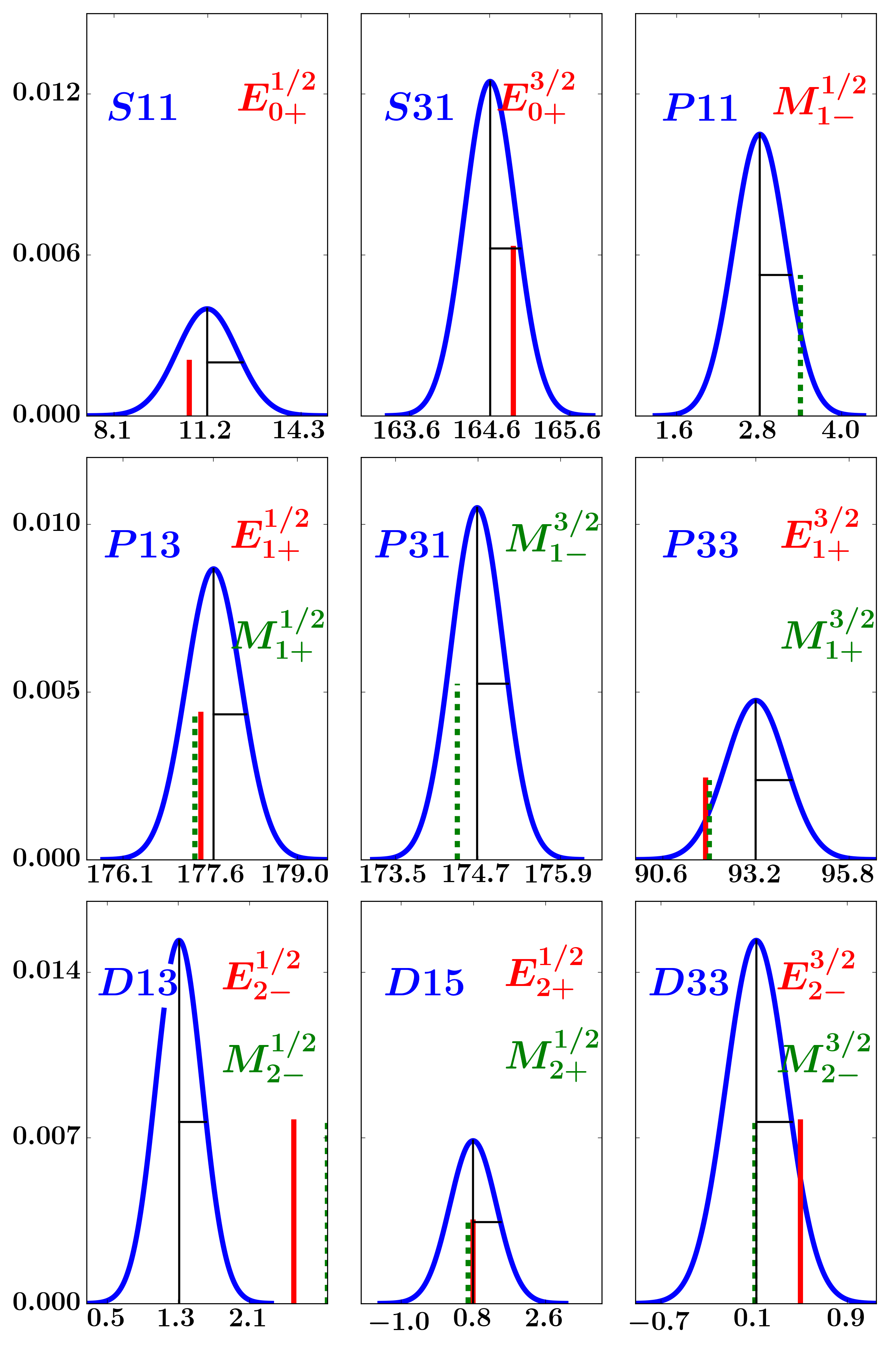
Figure 1: Plotted as normal distributions with $N[\mu,2\sigma]$ are the nine reported pion-nucleon scattering phase shifts of the single energy analysis WI08 [15] at $W_{cm}=1234.5$ $MeV$. Vertical lines show the MAID07 model values [16] for the corresponding pion photoproduction multipole phases ($\pm n\pi$), coded as red-continuous line for the Electric multipoles and green-dotted line for the Magnetic. The distributions are normalized to unity and are given in degrees.

Fig. 1 shows the nine $\pi N$ phases reported in ref. [12] as part of the WI08 partial wave analysis at $W=1235$ $MeV$ at the photon point. The exact numerical values are available online [15]. Each phase is plotted as a Gaussian, $N[\mu,2\sigma]$, with the same mean value ($\mu$) and double the statistical uncertainty ($\sigma$) derived from the experimental $\pi N$ data. The MAID07 model prediction [16] for the corresponding pion photoproduction multipole phases ($\pm n\pi$), at the same kinematics, is also shown. The $\pi N$ phases are known with limited accuracy, and although multipole analyses use them as if they are known with infinite precision, the effect of this uncertainty on the extracted multipoles has not been explored yet. Using the Athens Model Independent Analysis Scheme (AMIAS) we achieve this by constraining the phases within their experimentally determined uncertainty, making the analysis Bayessian.

The following sections are organized as follows: In Sec. 2 we discuss the methodology for multipole extraction with the AMIAS and the inclusion of parameters with known uncertainties. In Sec. 3 we detail the creation of pion photoproduction pseudodata of predetermined statistical precision. The multipole content of those pseudodata is derived in Sec. 4 validating the methodology described in Sec. 2. In Sec. 5 we apply the same methodology for a re-analysis of the Bates/Mainz electroproduction data [10] measured at $Q^{2}=0.127$ $GeV^{2}/c^{2}$ and $W=1232$ $MeV$. Concluding remarks are given in Sec. 6.

2 Methodology

The methodology employed is the implementation of the Chew, Goldenberg, Low and Nambu (CGLN) theoretical framework [17] for single energy multipole analyses in the Athens Model Independent Analysis Scheme (AMIAS) [18, 19]. The AMIAS method is based on statistical concepts and relies heavily on Monte Carlo and simulation techniques, and it thus requires High Performance Computing as it is computationally intensive. The method identifies and determines with maximal precision parameters that are sensitive to the data by yielding their Probability Distribution Functions (PDF). The AMIAS is computationally robust and numerically stable. It has been successfully applied in the analysis of data from nucleon photo-and electroproduction resonance [7, 18, 20], lattice QCD simulations [21] and medical imaging [22].

AMIAS requires that the parameters to be extracted from the experimental data are explicitly linked via a theory or a model [18]. In the case of pion photoproduction this requirement is provided by the CGLN theory as in ref. [7] and in the case of electroproduction as in ref. [18]. The multipoles are connected to the pion photoproduction observables via the CGLN [17] amplitudes $\left(F_{i},i=1,6\right)$:20pt

$$\begin{split}F_{1}={}&\sum_{l=0}^{\infty}[\left(lM_{l+}+E_{l+}\right)P^{\prime}_{l+1}(x)\\ &+\left(\left(l+1\right)M_{l-}+E_{l-}\right)P^{\prime}_{l-1}(x)]\end{split}$$ (2)

$$F_{2}={}\sum_{l=1}^{\infty}\left[\left(l+1\right)M_{l+}+lM_{l-}\right]P^{\prime}_{l}(x)$$ (3)

$$\begin{split}F_{3}={}&\sum_{l=1}^{\infty}[\left(E_{l+}-M_{l+}\right)P^{\prime\prime}_{l+1}(x)\\ &+\left(E_{l-}+M_{l-}\right)P^{\prime\prime}_{l-1}(x)]\end{split}$$ (4)

$$F_{4}={}\sum_{l=2}^{\infty}\left[M_{l+}-E_{l+}-M_{l-}-E_{l-}\right]P^{\prime\prime}_{l}(x)$$ (5)

$$F_{5}={}\sum_{l=0}^{\infty}\left[(l+1)L_{l+}P^{\prime}_{l+1}(x)-lL_{l-}P^{\prime}_{l-1}(x)\right]$$ (6)

$$F_{6}={}\sum_{l=1}^{\infty}\left[lL_{l-}-(l+1)L_{l+}\right]P^{\prime}_{l}(x)$$ (7)

where $x=\cos(\theta)$ is the cosine of the scattering angle and $P^{\prime}_{l}$ are the derivatives of the Legendre polynomials. Multipoles $A_{l\pm}=\{E_{l\pm},M_{l\pm},L_{l\pm}\}$ refer to the electric, magnetic or longitudinal nature of the photon respectively. At the real photon point, longitudinal degrees of freedom in the photon’s polarization vanish identically and the $\gamma N\to\pi N$ reaction is described solely by the CGLN amplitudes $F_{1}$ to $F_{4}$.

From isospin conservation in the pion-nucleon system it follows that the multipoles can be expressed in terms of definite isospin [23, 24], namely, the $A^{1/2}$ and $A^{3/2}$ multipoles. These are obtained from the reaction channel multipoles and the relations [24]:

$$A^{1/2} ={}\frac{A_{p\pi^{0}}}{3}+\frac{\sqrt{2}A_{n\pi^{+}}}{3}, A^{3/2} ={}A_{p\pi^{0}}-\frac{A_{n\pi^{+}}}{\sqrt{2}}$$ (8)

In contrast to the standard practice adhered up to now where the multipole phases are considered as if known with infinite precision [5, 10] and therefore treated as fixed parameters of the problem we allow those phases to vary within their experimentally determined uncertainty obtained from $\pi N$ experiments. This allows the prior knowledge on the multipole phases to be incorporated in the analysis.

To ascertain the magnitude of the effect this phase variation induces on the derived multipoles we examine three sets of pseudodata where each set was created with predetermined and increasing statistical precision. For each pseudodata set three multipole analyses were performed differentiated by the manner in which the multipole phases were treated; during the first analysis phases were fixed to the values of the generating model, during the second analysis phases were fixed to the SAID-WI08 [12, 15] model dependent analysis values and during the third multipole phases were allowed to vary with Gaussian weight, with mean value and twice the standard deviation of that reported by the SAID-WI08 single energy solution [12, 15]. In implementing the phase variation, and according to eq. 1, we imposed that during the variation procedure all multipoles with the same quantum numbers $I,l,J$ had the exact same phase $\pm\pi$. In contrast, multipole phases with different quantum numbers were varied independently.

3 Creation of pseudodata

20pt

$$d\sigma_{0} =\operatorname{Re}\left[F_{1}^{*}F_{1}+F_{2}^{*}F_{2}+\sin^{2}\theta\left(F_{3}^{*}F_{3}/2+F_{4}^{*}F_{4}/2+F_{2}^{*}F_{3}+F_{1}^{*}F_{4}+\cos\theta F_{3}^{*}F_{4}\right)-2\cos\theta F_{1}^{*}F_{2}\right]\rho$$

$$\hat{\Sigma} =-\sin^{2}\theta\operatorname{Re}\left[\left(F_{3}^{*}F_{3}+F_{4}^{*}F_{4}\right)/2+F_{2}^{*}F_{3}+F_{1}^{*}F_{4}+\cos\theta F_{3}^{*}F_{4}\right]\rho$$

$$\hat{T} =\sin\theta\operatorname{Im}\left[F_{1}^{*}F_{3}-F_{2}^{*}F_{4}+\cos\theta\left(F_{1}^{*}F_{4}-F_{2}^{*}F_{3}\right)-\sin^{2}\theta F_{3}^{*}F_{4}\right]\rho$$

$$\hat{P} =-\sin\theta\operatorname{Im}\left[2F_{1}^{*}F_{2}+F_{1}^{*}F_{3}-F_{2}^{*}F_{4}-\cos\theta\left(F_{2}^{*}F_{3}-F_{1}^{*}F_{4}\right)-sin^{2}\theta F_{3}^{*}F_{4}\right]\rho$$

$$\hat{E} =\operatorname{Re}\left[F_{1}^{*}F_{1}+F_{2}^{*}F_{2}-2\cos\theta F_{1}^{*}F_{2}+\sin^{2}\theta\left(F_{2}^{*}F_{3}+F_{1}^{*}F_{4}\right)\right]\rho$$

$$\hat{F} =\sin\theta\operatorname{Re}\left[F_{1}^{*}F_{3}-F_{2}^{*}F_{4}-\cos\theta\left(F_{2}^{*}F_{3}-F_{1}^{*}F_{4}\right)\right]\rho$$

$$\hat{G} =\sin^{2}\theta\operatorname{Im}\left[F_{2}^{*}F_{3}+F_{1}^{*}F_{4}\right]\rho$$

$$\hat{H} =\sin\theta\operatorname{Im}\left[2F_{1}^{*}F_{2}+F_{1}^{*}F_{3}-F_{2}^{*}F_{4}+\cos\theta\left(F_{1}^{*}F_{4}-F_{2}^{*}F_{3}\right)\right]\rho$$

Table 1: The CGLN content of the four single ($d\sigma_{0}$, $\hat{\Sigma}$, $\hat{T}$, $\hat{P}$) and four beam-target ($\hat{E}$, $\hat{F}$,$\hat{G}$, $\hat{H}$) polarization observables. The definitions $\rho=q/k$ and $\hat{O}=O/d\sigma_{0}$ are used. Angle $\theta$ is the center of mass scattering angle.

We have created pseudodata for the four single $(d\sigma_{0}$, $\hat{\Sigma}$, $\hat{T}$, $\hat{P})$ and four double beam-target $(\hat{E}$, $\hat{F}$, $\hat{G}$, $\hat{H})$ polarization observables for the $\gamma p\to p\pi^{0}$ and $\gamma p\to n\pi^{+}$ reactions. The definitions used for the observables are the same as in ref. [13]. To create the pseudodata the MAID07 multipole solution at the photon point and at center mass energy $W=1234.5$ $MeV$ was inserted in the CGLN multipole series, Eqs. 2-5, which were then used to construct the photoproduction observables defined in Table 1. A schematic of this “forward procedure” is given in Fig. 2. The observables were subsequently randomized according to the process: 20pt

$$\begin{split}O_{i}^{k}=&{}O_{i}^{k}+N[\mu,\sigma]\cdot O_{i}^{k}\\ \sigma_{O_{i}^{k}}=&{}N[\mu,\sigma]\cdot O_{i}^{k}\end{split}$$ (9)

where $O$ is the MAID07 model prediction, $k$ distinguishes between each of the spin observables, $i$ labels the angle, $N[\mu,\sigma]$ is a normal distribution with known mean $(\mu)$ and standard deviation $\sigma$ and $\sigma_{O_{i}^{k}}$ is the uncertainty attributed to the $i^{th}$ angular measurement of the $k^{th}$ observable.

Using Eq. 9 we created 9000 sets of pseudodata. Each pseudodata set consisted of $288$ datapoints; $18$ evenly spaced angular measurements in the dynamical region $\theta_{cm}\in[5^{\circ}:175^{\circ}]$ for each of the eight polarization observables listed in Table 1 for each proton target reaction. The angle $\theta_{cm}$ is defined as the angle between the incoming photon and the produced pion in the center of mass frame.

The generated values and uncertainties of the pseudodata sets are shown to have the required behavior [25, 26]. by examining the resulting $\chi^{2}$ distribution. The $\chi^{2}$ distribution resulting by comparing each dataset to the generator, shown in Fig. 3, is correctly described by the $\chi^{2}$ distribution with degrees of freedom equal to the number of datapoints $(=288)$ of the datasets.

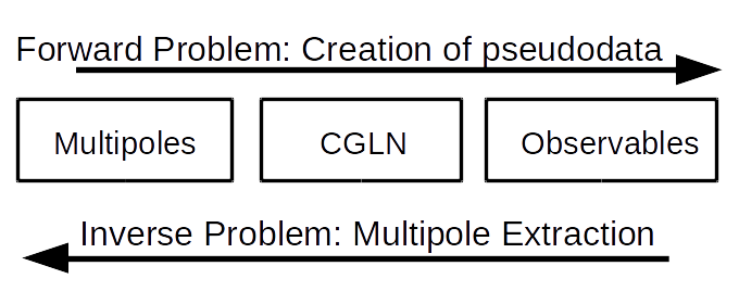
Figure 2: Multipole extraction in nucleon resonance photoproduction is an inverse problem in which the parameters to be extracted (multipoles) are connected to the experimental quantities via the CGLN formalism. To create pseudodata a forward procedure is followed in which known multipole input is used to form the CGLN amplitudes and subsequently the photoproduction observables.

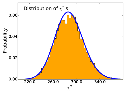
Figure 3: Histogram of the resulting $\chi^{2}$s as the generating model is passed without fitting through each dataset. Each dataset contains 288 datapoints. The histogram is described accurately by a $\chi^{2}$ distribution of degrees of freedom equal to the number of datapoints of each set.

The methodology followed in creating the pseudodata through eq. 9 allows to control the precision of the generated pseudodata. Three distinct classes of pseudodata were created; each class featuring pseudodata of statistical uncertainty a) $2.0$, b) $1.0$ and c) $0.16$ times the statistical uncertainty of the most precise pion photoproduction data [27] available to date. Fig. 4 show pseudodata for the differential cross section ($d\sigma_{0}/d\Omega$), the beam asymmetry ($\hat{\Sigma}$), the target asymmetry ($\hat{T}$) and the recoil target asymmetry ($\hat{P}$) for the two proton target reactions. The blue circles are used for pseudodata of relative uncertainty $2.0$, the green diamonds for pseudodata of relative uncertainty $1.0$ and the black triangles for relative uncertainty $0.16$. The continuous magenta curve is the generator. The pseudodata present some qualitative similarities to experimental data; the forward peak in the $\gamma\pi\to n\pi^{+}$ differential cross section, the absence of such peak in the $\gamma\pi\to p\pi^{0}$ differential cross section and larger uncertainties in the very forward and backward angles. The generated pseudodata also provide spin observables which have never been measured before, e.g. the beam-target $\hat{E}$, and full angular coverage.

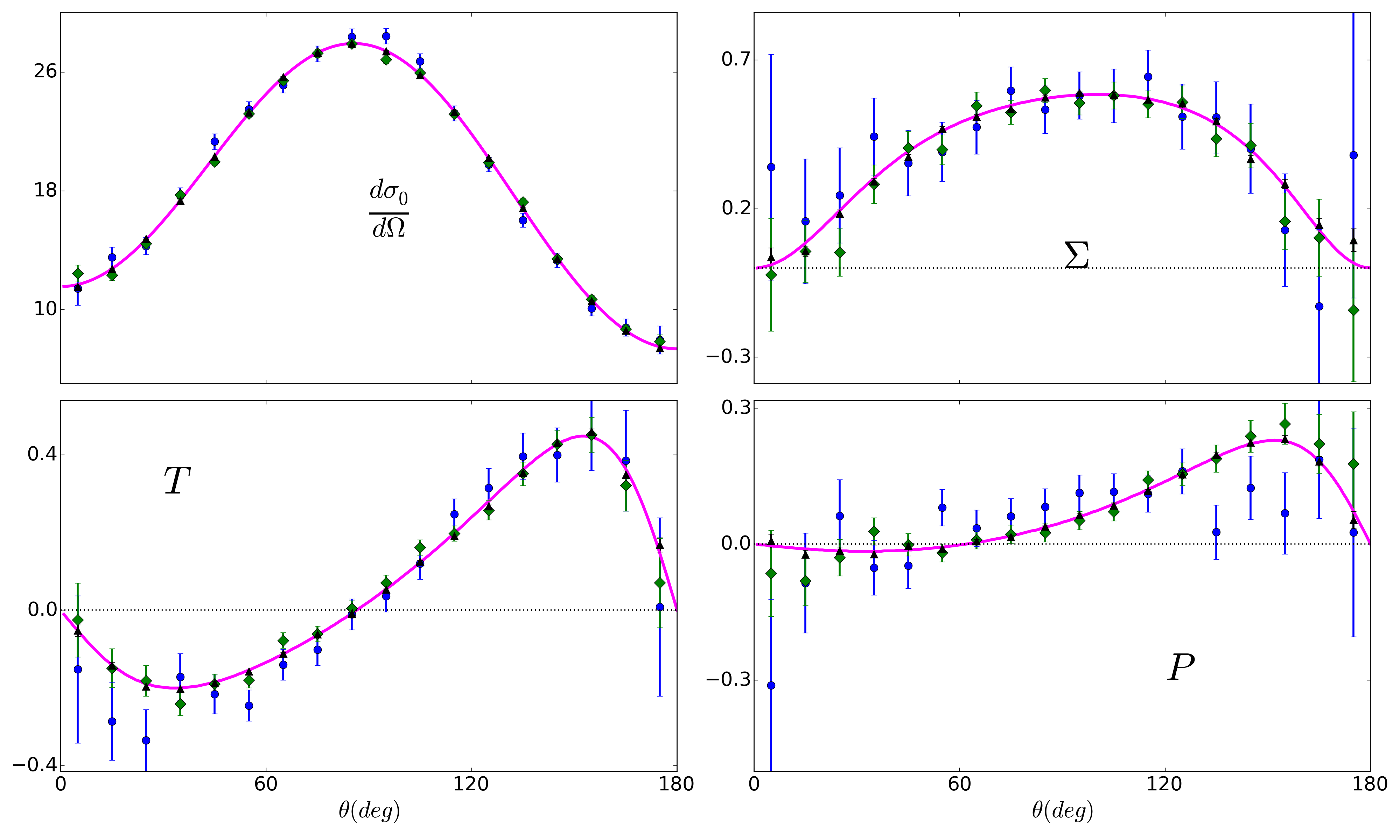
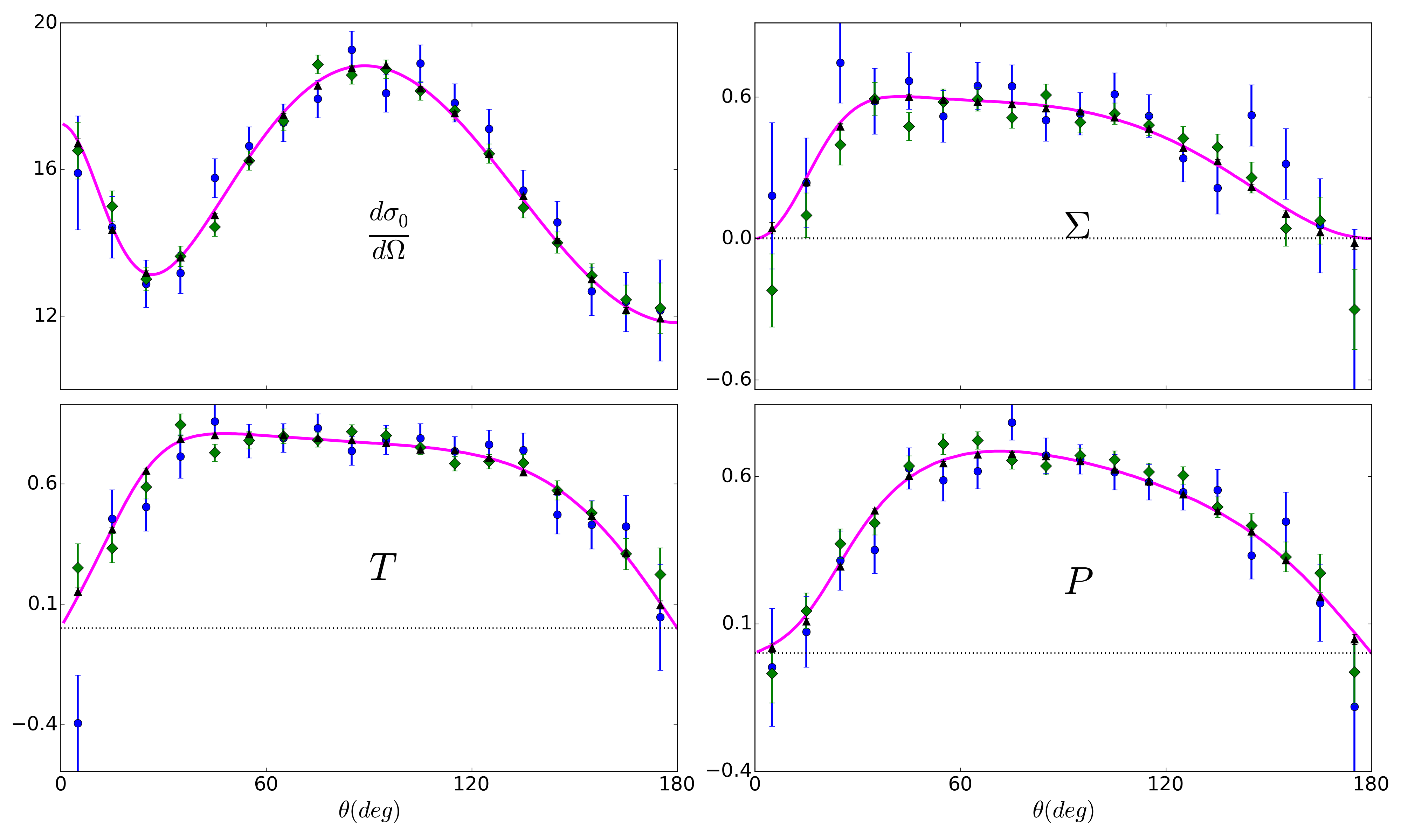
Figure 4: Illustration of the three sets of pseudodata with increasing precision for the differential cross section and the three single spin observables of the $\gamma p\to p\pi^{0}$ reaction (top four panels) and the $\gamma p\to n\pi^{+}$ reaction (bottom four panels). With blue circles are pseudodata of relative precision $2.0$, with green diamonds of relative precision $1.0$ and with black triangles of relative precision $0.16$. The precision of each dataset is given in relation to the precision of current experimental measurements [7, 27]. The continuous magenta curve is the MAID07 prediction (generator). The differential cross sections are given in units of $10^{-3}/m_{\pi}$.

4 Results

We applied the methodology presented in Sec. 2 to the pseudodata and we extracted values for all multipole amplitudes with relative angular momentum $\ell\leq 2$. Higher multipoles and up to all orders were frozen to the generating model values. The multipole amplitude PDFs derived from the AMIAS analyses were fitted with Gaussians and numerical results were extracted. Table LABEL:tab:fw_paper_tab_moduli lists the mean value $\pm 34\%$ uncertainty ($1\sigma$) for the derived multipoles for two distinct analyses: Column “MD07” and “W108” refer to analyses where the multipole phases were fixed to the MAID07 values (which is the generating model) or the WI08 solution respectively. Column “Varied” denotes analyses where the multipole phases were varied in a Gaussian manner with $N[\mu,2\sigma]$ where the mean value is taken from the WI08 $W$-dependent solution and the standard deviation, $\sigma$, the derived uncertainty of the WI08 single energy fit.

The derived multipole values and uncertainties are in good statistical agreement with the generator input. The derived multipole uncertainty from each pseudodata set for the analyses with the phases fixed, listed as “MD07” and “W108” in Table LABEL:tab:fw_paper_tab_moduli, is reduced according to the statistical precision of each set. The pseudodata sets, Set A, Set B and Set C were created with relative uncertainties $2.0$, $1.0$, and $0.16$ respectively. This is reflected in our results as the uncertainty associated with a specific multipole amplitude derived from Set A is reduced by a factor of $2.0$ and $12.5$ when derived from Sets B and C respectively. This behavior indicates that the AMIAS method yields exact uncertainties with a precise statistical meaning [18, 19]. Fig. 5 shows the PDFs of some selected amplitudes derived from the analysis of each pseudodata set with the multipole phases fixed to the MAID07 (generator) values. As expected the derived uncertainty of each multipole amplitude is seen to decrease according to the statistical precision of the analyzed pseudodata.

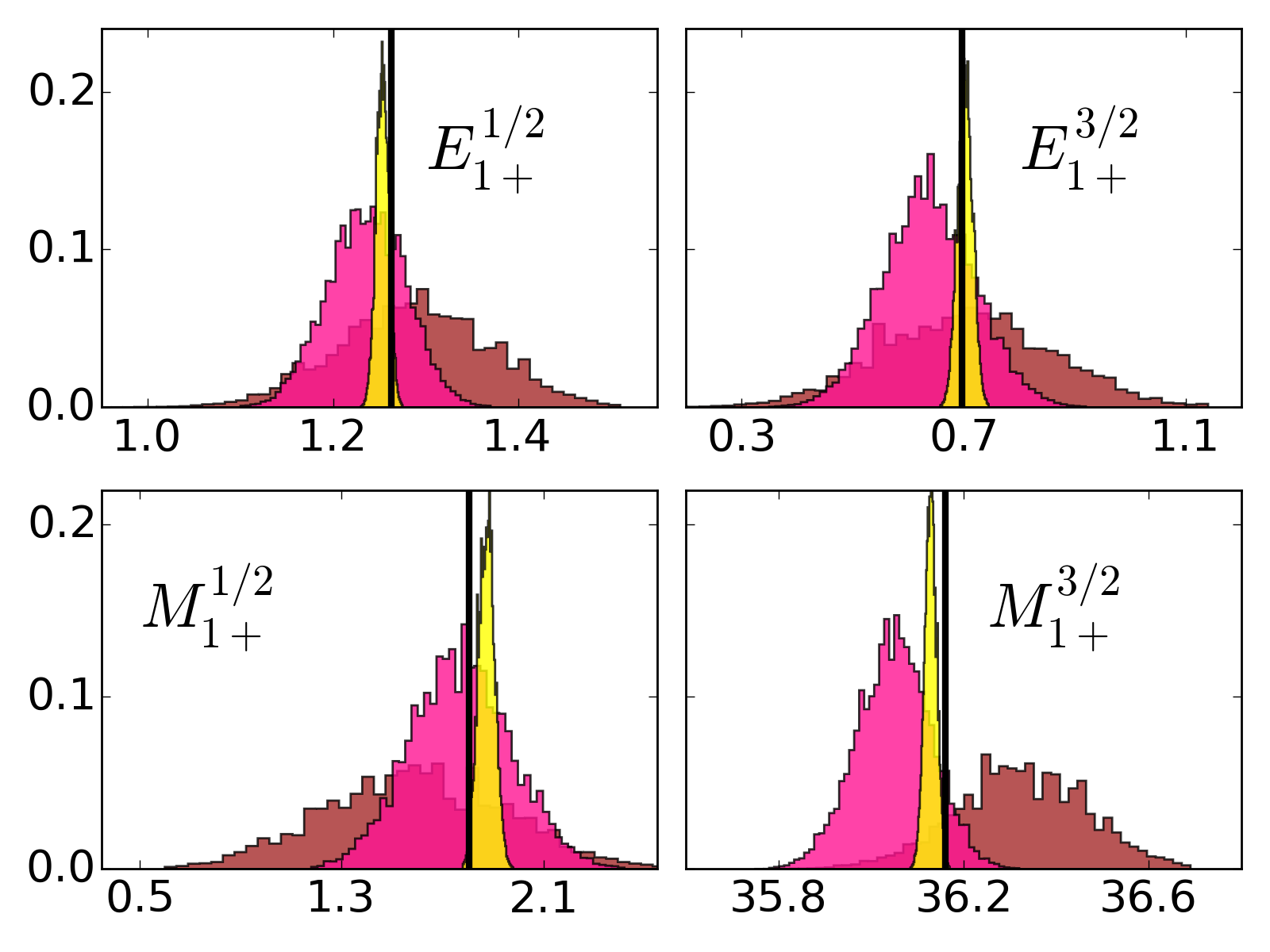
Figure 5: Probability Distribution Functions for the moduli of selected amplitudes derived from set A (brown), set B (magenta) and set C (yellow). The black vertical lines are the generator values (MAID07). Amplitudes are given in units of $10^{-3}/m_{\pi}$.

Regarding the analyses of the pseudodata sets A and B, which are characterized by uncertainties greater or equal to current experimental data, the derived results are statistically equivalent whether the analysis was carried with the multipole phases fixed to the generator values (MAID07), to the WI08 solution, or they were allowed to vary within the allowed experimental uncertainty. This is exhibited in Fig. 6 for the case of the $M_{1+}^{1/2}$ amplitude. It demonstrates that data of the currently available precision are not sensitive to such small changes or variations in the multipole phase. The standard practice in multipole analyses, to treat these phases as if known with infinite precision, does not induce additional model bias to the derived multipoles. Regarding the analyses of set C we note significant differences in the derived multipole mean values when phases change from the MAID07 values to the WI08 solution while the derived uncertainty remains unchanged. When the multipole phases are allowed to vary the derived multipole mean values are shifted while their associated uncertainty is increased. This increase is more prominent in the background multipole amplitudes $M_{1+}^{1/2}$ and $E_{0+}^{3/2}$. Fig. 6 shows this behavior for the case of the $M_{1+}^{1/2}$ amplitude.

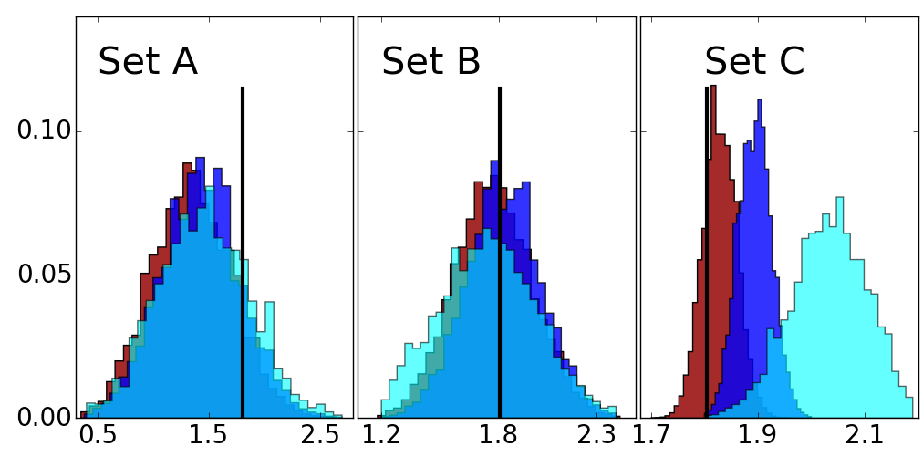
Figure 6: Probability Distribution Functions (PDFs) for the modulus of $M_{1+}^{1/2}$ derived from different pseudodata sets, each with increasing statistical precision. The PDFs are color coded according to the treatment of multipole phases during each analysis; brown (phases fixed to MAID07), blue (phases fixed to SAID-WI08) and cyan (phases varied with Gaussian weight. The black vertical lines is the generator value (MAID07). Amplitudes are given in units of $10^{-3}/m_{\pi}$.

For the analyses with “Varied” phases known, Normal distributions were utilized for the phase randomization. The analyses of pseudodata sets A and B yield phases nearly identical to the Normal distributions used for the phase variation. This indicates that data of such precision do not exhibit sensitivity to the magnitude of the phase variation we imposed. The derived phases from set C, the most precise analyzed pseudodata set, emerge significantly narrower than the Normal distributions utilized to vary them. Fig. 7 shows the PDF of the $E_{0+}^{1/2}$ phase derived from each pseudodata set. The phase PDFs derived from set A and B exactly match the distribution used to vary the phase and which is marked by a black continuous curve. The $E_{0+}^{1/2}$ phase derived from set C emerges much narrower.

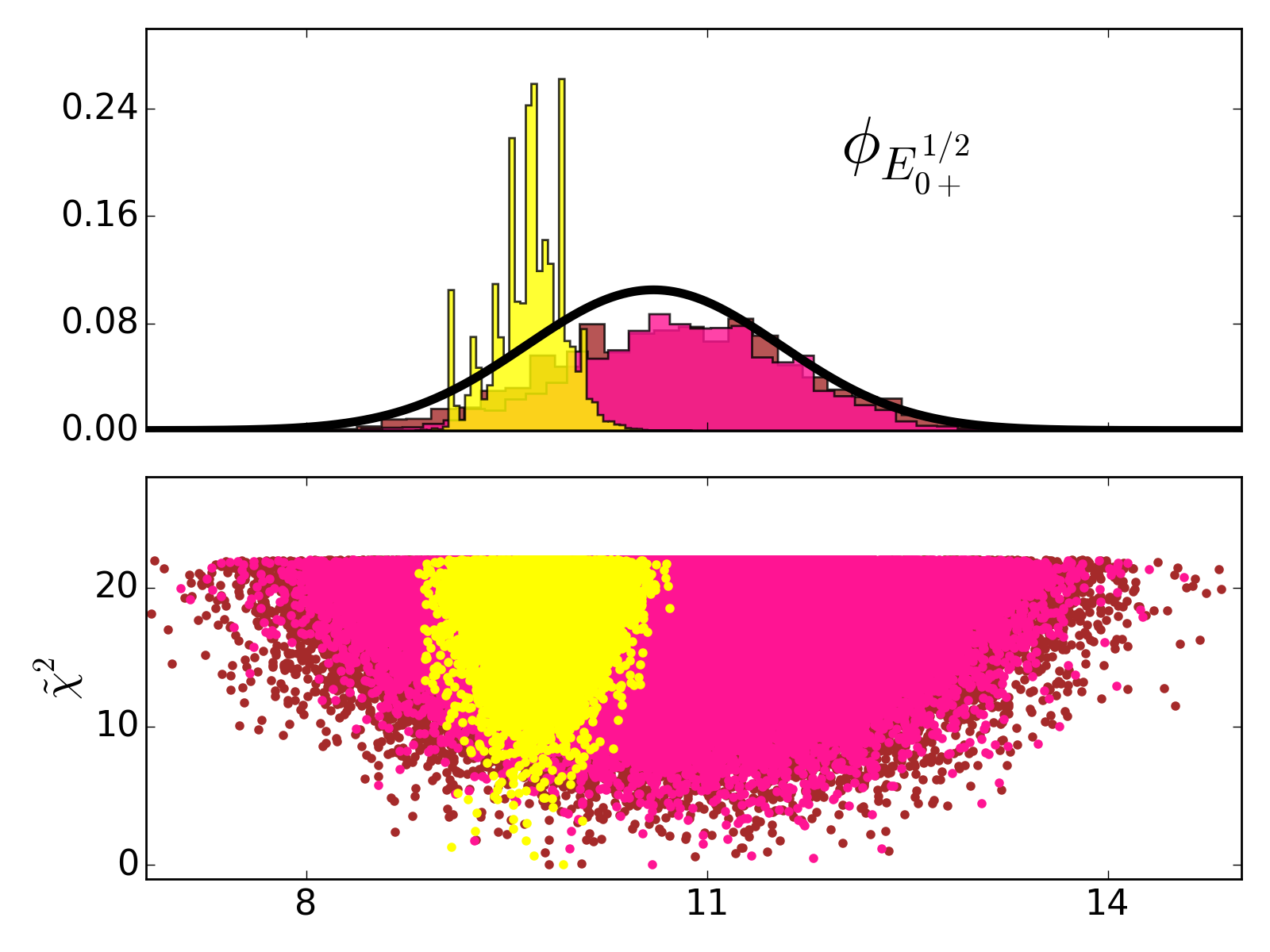
Figure 7: Top: Probability Distribution Functions normalized for the phase of $E_{0+}^{1/2}$ derived from set A (brown), set B (magenta) and set C (yellow). Phases are given in degrees. The black Normal is the distribution used to sample the MC space. Bottom: Scatter plot of $\tilde{\chi}^{2}$ VS $\phi_{E_{0+}^{1/2}}$ where $\tilde{\chi}^{2}=\chi^{2}-\chi^{2}_{min}$.

5 Example: Application to the Bates and Mainz data at $Q^{2}=0.127$ $(GeV/c)^{2}$

The methodology of Sec. 2 was applied for a re-analysis of the $H(e,e^{\prime},p)\pi^{0}$ Bates/Mainz measurements performed at $Q^{2}=0.127$ $GeV^{2}/c^{2}$ and $W=1232$ $MeV$. The detailed description and analysis of this data can be found in ref. [10]. The data set consists of cross section results for $\sigma_{TT}$, $\sigma_{LT}$, $\sigma_{0}$, $\sigma_{E2}$ and the polarized beam cross section $\sigma_{LT^{\prime}}$. The observables are defined as in ref. [24].

As the data concern $\gamma p\to p\pi^{0}$ measurements, model input (MAID07) was used to allow the isospin separation of multipoles and only few multipoles were derived. The derived parameters are the $l=0$ charge multipole amplitudes (the $A_{p\pi^{0}}$ multipoles of Eq. 8) and the $l=1$ resonant multipole amplitudes with isospin $I=3/2$. The $I=1/2$ multipoles were fixed to the MAID07 model values. We performed two new analyses of the data: in the first, the multipole phases were fixed to the $\pi N$ values [15]; in the second the $P_{33}$ phase was varied with Gaussian weight, with mean value the $\pi N$ scattering phase shift value and five times the experimental standard deviation ($\sigma$) of the scattering phase shift. The derived multipoles, which are listed in Table 2, were (statistically) identical in both cases; the phase variation did not induce any changes to the derived multipole amplitudes. Our results are in good agreement with earlier analyses of the same data [10, 18]. The Electric-to-Magnetic and Coulomb-to-Magnetic ratios, EMR and CMR respectively, are also given. These are defined as $EMR=E_{1+}^{3/2}/M_{1+}^{3/2}$ and $CMR=E_{1+}^{3/2}/S_{1+}^{3/2}$, where the Coulomb multipole $S_{1+}^{3/2}$ is connected to the longitudinal multipole, the photon’s momentum $q$ and the photon’s energy $\omega$ through the relation $S_{1+}^{3/2}=\frac{\vec{q}_{cm}}{\omega_{cm}}L_{1+}^{3/2}$. EMR and CMR serve as the accepted gauge of the magnitude of the deformation of the proton [28].

Table 2: Moduli of extracted amplitudes from the Bates/Mainz data. Results are with the phases fixed to $\pi N$ values [15] and with a $5\sigma$ Gaussian variation of the $P_{33}$ phase.

Multipole	Fixed	Varied	Ref. [10]
$I^{3/2}$ multipole amplitudes
$M_{1+}$	40.0 $\pm$ 0.8	40.0 $\pm$ 0.8	$41.4\pm 0.3$
$E_{1+}$	1.1 $\pm$ 0.3	1.1 $\pm$ 0.3	$0.95\pm 0.12$
$L_{1+}$	1.08 $\pm$ 0.13	1.09 $\pm$ 0.13	$1.26\pm 0.08$
Reaction channel multipole amplitudes
$E_{0+}$	3.3 $\pm$ 1.0	3.2 $\pm$ 1.0	2.9
$L_{0+}$	1.5 $\pm$ 0.5	1.6 $\pm$ 0.5	2.3
Ratios
$EMR(\%)$	$-2.8\pm 0.8$	$-2.8\pm 0.8$	$-2.3\pm 0.3$
$CMR(\%)$	$-5.5\pm 0.7$	$-5.5\pm 0.7$	$-6.1\pm 0.2$

6 Summary and Conclusions

Using the AMIAS methodology we explored the possible influence of the use of the Fermi-Watson theorem in pion photoproduction analyses. The current practice of using fixed (with no uncertainty) values was examined and compared to analyses where the $\pi N$ phase values and their uncertainty were used as prior knowledge. The AMIAS was used for the first time to allow prior knowledge to be incorporated into experimental analyses. Sets of pseudodata of increasing statistical precision were analyzed and their multipole content was derived. In the case of pseudodata of comparable statistical precision to the most recent pion photoproduction data the derived multipoles emerged nearly identical in mean value and uncertainty. The experimental phase uncertainty induced significant changes in the derived multipole amplitude PDFs when the analyzed pseudodata were created with precision six times the statistical precision of current experimental data.

The same methodology was applied to the $H(e,e^{\prime},p)\pi^{0}$ Bates/Mainz data measured at $Q^{2}=0.127$ $GeV^{2}/c^{2}$ and $W=1232$ $MeV$ where even a $5\sigma$ phase variation of the experimentally derived phase values did not induce any changes to the derived multipoles. We conclude that for the current precision of pion photo-and electroproduction data the $\pi N$ phases taken from pion-nucleon scattering as perfectly known is justified. However, for the new generation of data aspiring to distinguish among different models of nucleon structure, the type of analysis presented here where the experimentally derived phases are allowed to vary will need to be implemented.

References

- [1] G. Blanpied, M. Blecher, A. Caracappa et al. transition and proton polarizabilities from measurements of , , and . Phys. Rev. C, 64(2):025203, 2001.
- [2] K. M. Watson. Some general relations between the photoproduction and scattering of mesons. Phys. Rev., 95:228–236, Jul 1954.
- [3] G. Blanpied, M. Blecher, A. Caracappa et al. Transition from Simultaneous Measurements of and . Phys. Rev. Lett., 79(22):4337, 1997.
- [4] R. Beck, H. P. Krahn, J. Ahrens et al. Measurement of the Ratio in the Transition using the reaction and . Phys. Rev. Lett., 78:606–609, Jan 1997.
- [5] R. Beck, H. P. Krahn, J. Ahrens et al. Determination of the e 2/m 1 ratio in the n→ (1232) transition from a simultaneous measurement of p (→, p) 0 and p (→, +) n. Phys. Rev. C, 61(3):035204, 2000.
- [6] Martin Kotulla. Real Photon Experiments: and . In Shapes of Hadrons, volume 904, pages 203–212. AIP Publishing, 2007.
- [7] L. Markou, E. Stiliaris and C. N. Papanicolas. On hadron deformation: A model independent extraction of EMR from pion photoproduction data. Eur. Phys. J. A, 54(7):115, 2018.
- [8] V. V. Frolov, G. S. Adams, A. Ahmidouch et al. Electroproduction of the resonance at high momentum transfer. Phys. Rev. Lett., 82:45–48, Jan 1999.
- [9] C. Mertz, C. E. Vellidis, R. Alarcon et al. Search for quadrupole strength in the electroexcitation of the . Phys. Rev. Lett., 86:2963–2966, Apr 2001.
- [10] N. Sparveris, R. Alarcon, A. M. Bernstein et al. Investigation of the conjectured nucleon deformation at low momentum transfer. Phys. Rev. Lett., 94(2):022003, 2005.
- [11] S. Stave, M. O. Distler, I. Nakagawa, N. Sparveris et al. Lowest-Q2 measurement of the reaction: Probing the pionic contribution. Eur. Phys. J. A, 30(3):471–476, 2006.
- [12] RL Workman, RA Arndt, WJ Briscoe, MW Paris, and II Strakovsky. Parameterization dependence of t-matrix poles and eigenphases from a fit to n elastic scattering data. Phys. Rev. C, 86(3):035202, 2012.
- [13] R.L. Workman, M.W. Paris, W.J. Briscoe, L. Tiator, S. Schumann, M. Ostrick, and S.S. Kamalov. Model dependence of single-energy fits to pion photoproduction data. Eur. Phys. J. A, 47(11), 2011.
- [14] V Grushin. Photoproduction of Pions on Nucleons and Nuclei. In Proceedings of the Lebedev Physics Institute Academy of Science of the USSR, volume 186. Nova Science Publishers, New York and Budapest, 1989.
- [15] INS Data Analysis Center. http://gwdac.phys.gwu.edu/.
- [16] D. Drechsel, S. S. Kamalov, and L. Tiator. Unitary Isobar Model - MAID2007. Eur. Phys. J., A34:69–97, 2007.
- [17] GF Chew, ML Goldberger, FE Low, and Yoichiro Nambu. Relativistic dispersion relation approach to photomeson production. Phys. Rev., 106(6):1345, 1957.
- [18] E. Stiliaris and C. N. Papanicolas. Multipole extraction: A novel, model independent method. In AIP Conference Proceedings, volume 904, pages 257–268. AIP, 2007.
- [19] C. N. Papanicolas and E. Stiliaris. A novel method of data analysis for hadronic physics. arXiv preprint arXiv:1205.6505, 2012.
- [20] C. Alexandrou, C. N. Papanicolas, and M. Vanderhaeghen. Colloquium. Rev. Mod. Phys., 84:1231–1251, Sep 2012.
- [21] C. Alexandrou, T. Leontiou, C. N. Papanicolas, and E. Stiliaris. Novel analysis method for excited states in lattice QCD: The nucleon case. Phys. Rev. D, 91(1):014506, 2015.
- [22] C. N. Papanicolas, L. Koutsantonis, and E. Stiliaris. A Novel Analysis Method for Emmision Tomography.
- [23] F.A. Berends, A. Donnachie, and D.L. Weaver. Photoproduction and electroproduction of pions (i) dispersion relation theory. Nuclear Physics B, 4(1):1 – 53, 1967.
- [24] D Dreschsel and Lothar Tiator. Threshold pion photoproduction on nucleons. J. Phys. G: Nucl. Part. Phys., 18(3):449, 1992.
- [25] J. L. Friar and J. W. Negele. The determination of the nuclear charge distribution of from elastic electron scattering and muonic X-rays. Nucl. Phys. A, 212(1):93–137, 1973.
- [26] J. L. Friar and J. W. Negele. The determination of the nuclear charge distribution of 12c from elastic electron scattering. Nucl. Phys. A, 240(2):301–333, 1975.
- [27] P. Adlarson , J.R.M. Annand [A2 Collaboration]. Measurement of photoproduction on the proton at MAMI C. Phys. Rev. C, 92(2):024617, 2015.
- [28] C. N. Papanicolas and A. M. Bernstein. Shapes of hadrons. AIP conference proceedings. 2007.