High-energy and Very-high-energy emission from stellar-mass black holes moving in gaseous clouds

Abstract

We investigate the electron-positron pair cascade taking place in the magnetosphere of a rapidly rotating black hole. Because of the spacetime frame dragging, the Goldreich-Julian charge density changes sign in the vicinity of the event horizon, which leads to an occurrence of a magnetic-field aligned electric field, in the same way as the pulsar outer-magnetospheric accelerator. In this lepton accelerator, electrons and positrons are accelerated in the opposite directions, to emit copious gamma-rays via the curvature and inverse-Compton processes. We examine a stationary pair cascade, and show that a stellar-mass black hole moving in a gaseous cloud can emit a detectable very-high-energy flux, provided that the black hole is extremely rotating and that the distance is less than about 1 kpc. We argue that the gamma-ray image will have a point-like morphology, and demonstrate that their gamma-ray spectra have a broad peak around 0.01–1 GeV and a sharp peak around 0.1 TeV, that the accelerators become most luminous when the mass accretion rate becomes about 0.01% of the Eddington rate, and that the predicted gamma-ray flux little changes in a wide range of magnetospheric currents. An implication of the stability of such a stationary gap is discussed.

1 Introduction

By the Imaging Atmospheric Cherenkov Telescopes (IACTs), 76 very-high-energy (VHE) gamma-ray sources have been found on the Galactic Plane. So far, 19 of them have been identified as pulsar wind nebulae, 10 of them as supernova remnants adjacent to molecular clouds, whereas 36 of them are still remained unidentified. To consider the nature of such unidentified VHE sources in TeV energies, a hadronic cosmic-ray cascade model has been proposed (Ginzburg & Syrovatskii, 1964; Blandford & Eichler, 1987). In this model, charged particles such as protons are accelerated in the blast waves of a supernova remnant (SNR) and enter a dense molecular cloud. Then proton-proton collisions take place, leading to subsequent $\pi^{0}$ decays. The resultant $\gamma$-rays will show a single power-law spectrum between GeV and 100 TeV, reflecting the energy distribution of the parent cosmic rays. Its VHE emission morphology will become extended and the centroid of the VHE image will be located close to the peak of the gas density. Thus, if a VHE source positionally coincides with a dense molecular cloud with an extended morphology, and if the spectrum shows a single power-law between GeV and 100 TeV, it strongly suggest that the emission is due to the $\pi^{0}$ decay resulting from $p$-$p$ collisions.

On the other hand, there is an alternative scenario for a VHE emission from the magnetosphere of a rotating black hole (BH). This BH lepton accelerator model, or the BH-gap model, was first proposed by Beskin et al. (1992). Then Hirotani & Okamoto (1998); Neronov & Aharonian (2007); Rieger & Aharonian (2008); Levinson & Rieger (2011); Globus & Levinson (2014); Broderick & Tchekhovskoy (2015); Hirotani & Pu (2016); Levinson & Segev (2017) extended this pioneering work and quantified the BH-gap models. In the present paper, we proposed that a BH gap is activated when a rapidly rotating BH enters a molecular cloud or a gaseous cloud, and that its maximum possible $\gamma$-ray fluxes can be observable with the near-future IACTs such as the CTA, provided that the stellar-mass BH is extremely rotating and its distance is within 1 kpc. The morphology of such a gap emission is predicted to be point-like, and its spectrum will show two peaks around 0.1 GeV and 0.1 TeV.

On these grounds, to discriminate the physical origin of the VHE emissions, it is essential to examine if the source is extended or point-like, if the VHE peak coincides with the molecular density peak or not, and if the $\gamma$-ray spectrum is power-law or bimodal. We therefore briefly describe the observations of individual TeV sources in the next section. Then we describe the interactions between a BH and a gaseous cloud in § 3, a stationary BH gap model in § 4, and the results in § 5. In the final section, we highlight the difference of the present model from alternative $\gamma$-ray emission models from dense molecular clouds, and discuss the electrodynamical stability of stationary BH gap solutions.

2 Very-high-energy gamma-ray observations of the galactic plane

In this section, we describe the VHE observations of individual sources along the galactic plane, focusing on those associated with molecular clouds or unidentified.

It was pointed out that the VHE emission from HESS J1457-593 positionally coincides with a giant molecular cloud (GMC) complex, which overlaps the southern rim of SNR G318.2+01 with the typical $\mbox{H}_{2}$ number density of $40\mbox{ cm}^{-3}$ (Hofverberg et al., 2010). A two-dimensional Gaussian fit gives the source size of $\sigma_{1}=0.31^{\circ}$ and $\sigma_{2}=0.17^{\circ}$ along the major and minor axes, respectively. However, the source has a non-Gaussian morphology, which is likely further decomposed into two compact or point-like components in the north-south direction. Here, we define that a TeV source is compact if its angular size, $\sigma\equiv\sqrt{\sigma_{1}\sigma_{2}}$, is smaller than the angular resolution ($\sim 0.1^{\circ}$) of the present IACTs like the H. E. S. S., and define that a TeV source is point-like if $\sigma<0.5^{\circ}$. Therefore, if we observe the source with the new IACTs, Cherenkov Telescope Array (CTA), we may be able to decompose HESS J1457-593 into northern and southern compact and/or point-like components, both of which coincide with the peaks of ${}^{12}\mbox{CO}(J:1\rightarrow 0)$ line emission in the southern part of SNR G318.2+01. Interestingly, another dense molecular cloud exits about $0.5^{\circ}$ west of HESS J1457-593 and overlaps the southern rim of SNR G318.2+01; however, this dense molecular cloud does not show any detectable TeV emissions. It may be due to the propagation effect of the cosmic rays in the SNR shell; however, it may be due to a coincidental passage of one or two BHs in the GMC that positionally coincides with HESS J1457-593.

Subsequently, Aharonian et al. (2008a, b, c) reported the positional coincidence of six TeV sources, HESS J1714-385, HESS J1745-303, HESS J1801-233, HESS J1800-240A, B, and C with dense molecular clouds. HESS J1714-385 has a compact morphology with size $\sigma=0.07^{\circ}$ and positionally associated with an extended dense molecular clouds whose density is $1.5\times 10^{2}\mbox{ cm}^{-3}<n_{{\rm H}_{2}}<6.6\times 10^{2}\mbox{ cm}^{-3}$. However, the peak of the TeV emission resides in the valley between the two $\mbox{H}_{2}$ density peaks. This positional deviation from the molecular density peak may be due to the propagation effect of the CRs emitted from SNR 37A, or may be due to a passage of a BH in the molecular cloud. HESS J1745-303 has an extended morphology and show the VHE emission above 20 TeV; thus, we consider that the VHE photons are emitted via a hadronic interaction between CRs and the molecular clouds for this source. HESS J1801-233, HESS J1800-2400A and B are extended and roughly overlaps the density peaks of the molecular cloud whose averaged molecular density is $n_{{\rm H}_{2}}\sim 10^{3}\mbox{ cm}^{-3}$. Thus, VHE photons may be emitted by the interaction between CRs and molecular clouds in these three TeV sources. The remaining one TeV source, HESS J1800-2400C, has a point-like morphology with $\sigma=0.02^{\circ}$ and appear to be deviated from the peak of the molecular density. In short, among these six TeV sources that are positionally associated with dense molecular clouds, two sources, HESS J1714-385 and HESS J1800-2400C, have compact and point-like morphology, respectively. It is noteworthy that the centroids of their TeV emission deviate from the nearby peaks of molecular hydrogen column density. Therefore, if their emission morphology is found to be point-like with CTA, and if the VHE spectrum cuts off around 1 TeV (see § 5.3), the BH-gap scenario may account for these two VHE sources.

Following these pioneering works mentioned just above, de Wilt et al. (2017) carried out a systematic comparison between TeV sources and dense molecular gas along the galactic plane. They used published HESS data up to 2015 March and picked up 49 TeV sources with 11–15 mm radio observations of molecular emission lines. They found that 38 of the 49 sources are positionally associated with dense gas counterparts; specifically speaking, $\mbox{NH}_{3}\mbox{(1,1)}$ line emissions were detected from or adjacent to the 38 TeV sources. Moreover, out of unidentified 18 TeV sources, 12 of them are positionally associated with dense molecular clouds. Among these 12 TeV sources, 9 sources were fit with Gaussian model, 5 of which are found to have compact morphology. Specifically, HESS J1634-472, HESS J1804-216, and HESS J1834-087 have the sizes of $\sigma=0.11^{\circ}$, $0.20^{\circ}$, and $0.09^{\circ}$, respectively (Aharonian et al., 2006); thus, one of the three sources is compact. Also, HESS J1472-608, HESS J1626-490, HESS J1702-420, HESS J1708-410, HESS J1841-055, have $\sigma=0.056^{\circ}$, $0.083^{\circ}$, $0.212^{\circ}$, $0.069^{\circ}$, and $0.320^{\circ}$, respectively (Aharonian et al., 2008d); thus, three of the five sources are compact. Subsequently, HESS J1641-463 is also found to be compact with $\sigma=0.085^{\circ}$ (Abramowski et al., 2014). For the 38 TeV sources positionally associated with dense molecular clouds, the molecular hydrogen density is typically in the range $10^{3}\mbox{ cm}^{-3}<n_{{\rm H}_{2}}<10^{5}\mbox{ cm}^{-3}$. Among the 5 compact TeV sources that are positionally associated with dense molecular clouds, the centroid of HESS J1626-490 coincides with the molecular density peak; thus, this source may be due to the interaction between CRs and molecular clouds. However, there is a possibility that BH gaps emit the observed TeV photons for the remaining 4 compact sources, in addition to the point-like source HESS J1800-2400C. In what follows, we thus investigate if a stellar-mass BH can emit detectable TeV photons when they enter a gaseous cloud.

3 Black holes moving in a gaseous cloud

Before proceeding to the BH gap model, we must consider the mass accretion process when a BH moves in a dense gaseous cloud. Thus, in the subsequent three subsections, we briefly describe the giant molecular clouds (GMCs), formation of BHs, and the accretion process in a gaseous cloud.

3.1 Giant molecular clouds

Molecular clouds are generally gravitationally bound and occasionally contain several sites of star formation. Particularly, massive stars formed in a GMC can ionize the surrounding interstellar medium with their strong UV radiation. A combined action of such ionization, stellar winds, and supernova explosions, blow off the gases in a GMC, leaving an OB association adjacent to dense molecular clouds. In this section, we focus on the physical parameters in such dense molecular clouds, which may be traversed by a BH formed in a neighboring OB association.

The physical parameters (e.g., temperature and density) of a molecular cloud can be examined by observing the strength, width, and profile of radio emission lines of probe molecules. A typical GMC has gas kinematic temperature between $30$ K and $50$ K. Using the dense-gas tracers, ${\rm H}_{2}{\rm CO}$ and CS, we can infer the hydrogen molecule number density, $n_{{\rm H}_{2}}$ in the core of a GMC. A typical GMC core has the density $10^{4}\mbox{ cm}^{-3}<n_{{\rm H}_{2}}<10^{6}\mbox{ cm}^{-3}$, and mass between $10M_{\odot}$ and $10^{3}M_{\odot}$. Individual molecular clouds have lower densities, $10^{2}\mbox{ cm}^{-3}<n_{{\rm H}_{2}}<10^{5}\mbox{ cm}^{-3}$ and masses between $10^{3}M_{\odot}$ and $10^{6}M_{\odot}$. We use these values of $n_{{\rm H}_{2}}$ to estimate the mass accretion rate onto a BH in § 3.3.

3.2 Black hole formation in GMCs

To consider the passage of a stellar-mass BH in a dense molecular cloud, let us briefly comment on the massive star formation in a GMC. In a GMC, massive stars are formed in OB associations. A typical OB association contains $10^{1-2}$ high-mass stars of type O and B and $10^{2-3}$ stars of lower masses. The stellar line-of-sight velocity dispersion in an OB association is typically around $9\mbox{ km s}^{-1}$ and usually less than $20\mbox{ km s}^{-1}$ (Sitnik, 2003). The strong winds and the supernovae resulting from these associations, blow off the interstellar medium; thus, OB associations are found adjacent to molecular clouds (Blitz, 1980). Depending on the mass and metalicity, such high-mass, OB stars evolve into neutrons stars or BH after core collapse events. For example, if the progenitor has mass $M$ in $25M_{\odot}<M<40M_{\odot}$ with low or solar metalicity, it will evolve into a BH through a supernova explosion after the fall back of material onto an initial neutron star. In this case, the BH will acquire a certain kick velocity with respect to the star-forming region in the similar way as neutron stars. On the other hand, if it has $M>40M_{\odot}$ with low metalicity, it will evolve into a BH directly without a supernova explosion. These massive BHs will have smaller relative velocities with respect to the star-forming region compared to the lighter BHs formed through core-collapse supernovae. Nevertheless, we may expect that such BHs, whichever formed with or without supernovae, move into nearby dense molecular clouds. Thus, in the next subsection, we estimate the plasma accretion rate when such a stellar-mass BH enters a dense gaseous cloud.

3.3 Bondi accretion rate in the molecular cloud core

To estimate the accretion rate onto a BH, we examine the Bondi accretion rate when a BH moves in a gaseous cloud. To this end, we begin with comparing the sound speed in a typical molecular cloud and the relative velocity between the cloud and the BH.

The sound speed of a cloud with kinetic temperature $T$ (K) can be estimated by

$$C_{\rm s}\sim\sqrt{\frac{k_{\rm B}T}{m_{\rm p}}}=90\,T^{1/2}\mbox{ m s}^{-1},$$ (1)

where $k_{\rm B}$ refers to the Boltzmann constant, and $m_{p}$ the proton mass. For a typical GMC, we have $T<50$ K, and for a typical dark cloud, we have $T<20$ K. Thus, we obtain $C_{\rm s}<630\mbox{ m s}^{-1}$ as the upper limit of the sound speed in a molecular cloud.

A typical velocity $V$ of a BH relative to the cloud may be estimated by the kick velocity in a supernova explosion. For a neutron star, it is typically a few hundred kilometers per second. For a BH, a greater fraction of mass is expected to be turned into a compact object; so, we may expect the typical velocity is around $10^{2}\mbox{ km s}^{-1}$. Turbulent velocities measured from molecular line width are usually less than $10\mbox{ km s}^{-1}$, and relative velocities among smaller scale clouds are also within this small range. Thus, we can neglect such random or bulk motions and adopt the supernova kick velocity, $V\sim 10^{2}\mbox{ km s}^{-1}$, as the typical velocity of a BH with respect to the molecular clouds. If a heavier BH ($M>40M_{\odot}$) is formed without a supernova explosion, the relative velocity will be less than this value.

On these grounds, we can safely put $V\gg C_{\rm s}$. In this case, the flow becomes supersonic with respect to the BH and a shock wave is formed behind the hole. Accordingly, the gas particles within the Bondi radius (i.e., within the impact parameter) $r_{\rm B}\sim GM/V^{2}$ from the BH, are captured, falling onto the BH with the Bondi accretion rate, (Bondi & Hoyle, 1944)

$$\dot{M}_{\rm B}=4\pi\lambda(GM)^{2}V^{-3}\rho,$$ (2)

where $\rho$ denotes the mass density of the gas, and $\lambda$ is a constant of order unity. We have $\lambda=1.12$ and $0.25$ for an isothermal and adiabatic gas, respectively. Assuming molecular hydrogen gas, and normalizing with the Eddington accretion rate, we obtain the following dimensionless Bondi accretion rate,

$$\dot{m}_{\rm B}=5.39\times 10^{-9}\lambda n_{{\rm H}_{2}}M_{1}\left(\frac{\eta}{0.1}\right)^{-1}\left(\frac{V}{10^{2}\mbox{ km s}^{-1}}\right)^{-3},$$ (3)

where $n_{{\rm H}_{2}}$ is measured in $\mbox{cm}^{-3}$ unit, $\eta\sim 0.1$ denotes the radiation efficiency of the accretion flow, and $M_{1}\equiv M/(10M_{\odot})$.

Since the accreting gases have little angular momentum as a whole with respect to the BH, they form an accretion disk only within a radius that is much less than $r_{\rm B}$. Thus, we neglect the mass loss as a disk wind between $r_{\rm B}$ and the inner-most region, and evaluate the accretion rate near the BH, $\dot{m}$, with $\dot{m}_{\rm B}$. As will be shown in § 5.3, the gap of a stellar-mass BH becomes most luminous when $6\times 10^{-5}<\dot{m}<2\times 10^{-4}$. For $\dot{m}$ to reside in this range, a dense, isothermal molecular cloud core should have a density $n_{{\rm H}_{2}}>10^{4}\mbox{ cm}^{-3}$, if $V=100\mbox{km s}^{-1}$. If $V=50~{}\mbox{ km s}^{-1}$, however, a lower density, $n_{{\rm H}_{2}}>1.2\times 10^{3}\mbox{ cm}^{-3}$, is enough to activate the BH gap.

4 Magnetospheric lepton accelerator model

In this section, we formulate the BH gap model and examine the resultant gamma-ray emission when a stellar-mass BH moves in a dense molecular cloud. We quickly review the pulsar outer gap model in section 4.1, and apply it to BH magnetospheres in section 4.2, focusing on the improvements from previous works by the authors.

4.1 Pulsar outer-magnetospheric lepton accelerator model

The Large Area Telescope (LAT) aboard the Fermi space gamma-ray observatory has detected pulsed signals in high-energy (0.1 GeV-10 GeV) gamma-rays from more than 200 rotation-powered pulsars . Among them, 20 pulsars exhibit pulsed signals above 10 GeV, including 10 pulsars up to 25 GeV and other 2 pulsars above 50 GeV. Moreover, more than 99% of the LAT-detected young and millisecond pulsars exhibit phase-averaged spectra that are consistent with a pure-exponential or a sub-exponential cut off above the cut-off energies at a few GeV. What is more, 30% of these young pulsars show sub-exponential cut off, a slower decay than the pure-exponential functional form. These facts preclude the possibility of emissions from the inner magnetosphere as in the polar-cap scenario (Harding et al., 1978; Daugherty & Harding, 1982; Dermer, 1994; Timokhin & Arons, 2013; Timokhin & Harding, 2015), which predicts super-exponential cut off due to magnetic attenuation. That is, we can conclude that the pulsed emissions are mainly emitted from the outer magnetosphere, which is close to or outside the light cylinder.

One of the main scenarios of such outer-magnetospheric emissions is the outer-gap model (Cheng et al., 1986a, b; Chiang & Romani, 1992; Romani, 1996; Cheng et al., 2000; Hirotani, 2006). In the present paper, we apply this successful scenario to BH magnetospheres. Although the electrodynamics is mostly common between the pulsar outer-gap model and the present BH-gap model, there is a striking difference between them. In a pulsar magnetosphere, an outer gap arises because of the convex geometry of the dipolar-like magnetic field in the outer magnetosphere. However, in a BH magnetosphere, a gap arises because of the frame-dragging in the vicinity of the event horizon. We describe this BH-gap model below.

4.2 Black-hole inner-magnetospheric lepton accelerator model

4.2.1 Background spacetime geometry

In a rotating BH magnetosphere, electron-positron accelerator is formed in the direct vicinity of the event horizon. Thus, we start with describing the background spacetime in a fully general-relativistic way. We adopt the geometrized unit, putting $c=G=1$, where $c$ and $G$ denote the speed of light and the gravitational constant, respectively. Around a rotating BH, the spacetime geometry is described by the Kerr metric (Kerr, 1963). In the Boyer-Lindquist coordinates, it becomes (Boyer & Lindquist, 1967)

$$ds^{2}=g_{tt}dt^{2}+2g_{t\varphi}dtd\varphi+g_{\varphi\varphi}d\varphi^{2}+g_{rr}dr^{2}+g_{\theta\theta}d\theta^{2},$$ (4)

where

$$g_{tt}\equiv-\frac{\Delta-a^{2}\sin^{2}\theta}{\Sigma},\qquad g_{t\varphi}\equiv-\frac{2Mar\sin^{2}\theta}{\Sigma},$$ (5)

$$g_{\varphi\varphi}\equiv\frac{A\sin^{2}\theta}{\Sigma},\qquad g_{rr}\equiv\frac{\Sigma}{\Delta},\qquad g_{\theta\theta}\equiv\Sigma;$$ (6)

$\Delta\equiv r^{2}-2Mr+a^{2}$, $\Sigma\equiv r^{2}+a^{2}\cos^{2}\theta$, $A\equiv(r^{2}+a^{2})^{2}-\Delta a^{2}\sin^{2}\theta$. At the horizon, we obtain $\Delta=0$, which gives the horizon radius, $r_{\rm H}\equiv M+\sqrt{M^{2}-a^{2}}$, where $M$ corresponds to the gravitational radius, $r_{\rm g}\equiv GMc^{-2}=M$. The spin parameter $a$ becomes $a=M$ for a maximally rotating BH, and becomes $a=0$ for a non-rotating BH. The spacetime dragging frequency is given by $\omega(r,\theta)=-g_{t\varphi}/g_{\varphi\varphi}$, which decreases outwards as $\omega\propto r^{-3}$ at $r\gg r_{\rm g}=M$.

4.2.2 Poisson equation for the non-corotational potential

We assume that the non-corotational potential $\Phi$ depends on $t$ and $\varphi$ only through the form $\varphi-\Omega_{\rm F}t$, and put

$$F_{\mu t}+\Omega_{\rm F}F_{\mu\varphi}=-\partial_{\mu}\Phi(r,\theta,\varphi-\Omega_{\rm F}t),$$ (7)

where $\Omega_{\rm F}$ denotes the magnetic-field-line rotational angular frequency. We refer to such a solution as a ‘stationary’ solution in the present paper.

The Gauss’s law gives the Poisson equation that describes $\Phi$ in a three dimensional magnetosphere (Hirotani, 2006),

$$-\frac{1}{\sqrt{-g}}\partial_{\mu}\left(\frac{\sqrt{-g}}{\rho_{\rm w}^{2}}g^{\mu\nu}g_{\varphi\varphi}\partial_{\nu}\Phi\right)=4\pi(\rho-\rho_{{\rm GJ}}),$$ (8)

where the general-relativistic Goldreich-Julian (GJ) charge density is defined as (Hirotani, 2006)

$$\rho_{\rm GJ}\equiv\frac{1}{4\pi\sqrt{-g}}\partial_{\mu}\left[\frac{\sqrt{-g}}{\rho_{\rm w}^{2}}g^{\mu\nu}g_{\varphi\varphi}(\Omega_{\rm F}-\omega)F_{\varphi\nu}\right].$$ (9)

Far away from the horizon, $r\gg M$, equation (9) reduces to the ordinary, special-relativistic expression of the GJ charge density (Goldreich & Julian, 1969; Mestel, 1971),

$$\rho_{\rm GJ}\equiv-\frac{\mbox{\boldmath$\Omega$}\cdot\mbox{\boldmath$B$}}{2\pi c}+\frac{(\mbox{\boldmath$\Omega$}\times\mbox{\boldmath$r$})\cdot(\nabla\times\mbox{\boldmath$B$})}{4\pi c}.$$ (10)

Therefore, the corrections due to magnetospheric currents, which are expressed by the second term of eq. (10), are included in equation (9).

If the real charge density $\rho$ deviates from the rotationally induced GJ charge density, $\rho_{\rm GJ}$, in some region, equation (8) shows that $\Phi$ changes as a function of position. Thus, an acceleration electric field, $E_{\parallel}=-\partial\Phi/\partial s$, arises along the magnetic field line, where $s$ denotes the distance along the magnetic field line. A gap is defined as the spatial region in which $E_{\parallel}$ is non-vanishing. At the null charge surface, $\rho_{{\rm GJ}}$ changes sign by definition. Thus, a vacuum gap, in which $|\rho|\ll|\rho_{{\rm GJ}}|$, appears around the null-charge surface, because $\partial E_{\parallel}/\partial s$ should have opposite signs at the inner and outer boundaries (Chiang & Romani, 1992; Romani, 1996; Cheng et al., 2000). As an extension of the vacuum gap, a non-vacuum gap, in which $|\rho|$ becomes a good fraction of $|\rho_{{\rm GJ}}|$, also appears around the null-charge surface (§ 2.3.2 of HP 16), unless the injected current across either the inner or the outer boundary becomes a substantial fraction of the GJ value. If the injected current becomes non-negligible compared to the created current in the gap, the gap centroid position shifts from the null surface; however, the essential gap electrodynamics does not change.

In previous series of our papers (Hirotani & Pu, 2016; Hirotani et al., 2016b; Song et al., 2017), we have assumed $\Delta\ll M^{2}$ in Equation (8), expanding the left-hand side in the series of $\Delta/M^{2}$ and pick up only the leading orders. However, in the present paper, we discard this approximation, and consider all the terms that arise at $\Delta\sim M^{2}$ or $\Delta\gg M^{2}$.

It should be noted that $\rho_{\rm GJ}$ vanishes, and hence the null surface appears near the place where $\Omega_{\rm F}$ coincides with the space-time dragging angular frequency, $\omega$ (Beskin et al., 1992). The deviation of the null surface from this $\omega(r,\theta)=\Omega_{\rm F}$ surface is, indeed, small, as figure 1 of Hirotani & Okamoto (1998) indicates. Since $\omega$ can match $\Omega_{\rm F}$ only near the horizon, the null surface, and hence the gap generally appears within one or two gravitational radii above the horizon, irrespective of the BH mass.

4.2.3 Particle Boltzmann equations

We outline the Boltzmann equations of $e^{\pm}$’s, following Hirotani et al. (2017). Imposing a stationary condition, $\partial/\partial t+\Omega_{\rm F}\partial/\partial\phi=0,$ we obtain the following Boltzmann equations,

$$c\cos\chi\frac{\partial n_{\pm}}{\partial s}+\dot{p}\frac{\partial n_{\pm}}{\partial p}=\alpha(S_{{\rm IC},\pm}+S_{{\rm p},\pm}),$$ (11)

along each radial magnetic field line on the poloidal plane, where the upper and lower signs correspond to the positrons (with charge $q=+e$) and electrons ($q=-e$), respectively, and $p\equiv|\mbox{\boldmath$p$}|=m_{\rm e}c\sqrt{\gamma^{2}-1}$. The left-hand side is in $dt$ basis, where $t$ denotes the proper time of a distant static observer. Thus, the lapse $\alpha$ is multiplied in the right-hand side, because both $S_{\rm IC}$ and $S_{\rm p}$ are evaluated in the zero-angular-momentum observer (ZAMO). Dimensionless lepton distribution functions per magnetic flux tube are defined by

$$n_{\pm}\equiv\frac{2\pi ce}{\Omega_{\rm F}B}N_{\pm}(r,\theta,\gamma),$$ (12)

where $N_{+}$ and $N_{-}$ designate the distribution functions of positrons and electrons, respectively; $\gamma$ refers to these lepton’s Lorentz factor, and $B\equiv|\mbox{\boldmath$B$}|$. It is convenient to include the curvature emission as a friction term in the left-hand side; in this case, we obtain

$$\dot{p}\equiv qE_{\parallel}\cos\chi-\frac{P_{\rm SC}}{c},$$ (13)

where the pitch angle is assumed to be $\chi=0$ for outwardly moving positrons, and $\chi=\pi$ for inwardly moving electrons. The curvature radiation force is given by (e.g., Harding, 1981), $P_{\rm SC}/c=2e^{2}\gamma^{4}/(3R_{\rm c}{}^{2})$.

The IC collision terms are expressed as

$$S_{\rm IC} \equiv -\int_{\epsilon_{\gamma}<\gamma}d\epsilon_{\gamma}\eta_{\rm IC}^{\gamma}(\epsilon_{\gamma},\gamma,\mu_{\pm})n_{\pm}$$ (14)

$$+ \int_{\gamma_{i}>\gamma}d\gamma_{i}\eta_{\rm IC}^{\rm e}(\gamma_{i},\gamma,\mu_{\pm})n_{\pm},$$

where the IC redistribution function is defined by

$$\eta_{\rm IC}^{\gamma}\equiv(1-\beta\mu_{\pm})\int_{E_{\rm min}}^{E_{\rm max}}dE_{\rm s}\frac{dF_{\rm s}}{dE_{\rm s}}\frac{d\epsilon_{\gamma}^{\ast}}{d\epsilon_{\gamma}}\int_{-1}^{1}d\Omega_{\gamma}^{\ast}\frac{d\sigma_{\rm KN}^{\ast}}{d\epsilon_{\gamma}^{\ast}d\Omega_{\gamma}^{\ast}},$$ (15)

$m_{\rm e}c^{2}\epsilon_{\gamma}$ denotes the upscattered $\gamma$-ray energy. The asterisk denotes that the quantity evaluated in the electron (or positron) rest frame and $d\sigma_{\rm KN}^{\ast}/d\epsilon_{\gamma}^{\ast}d\Omega_{\gamma}^{\ast}$ denotes the Klein-Nishina differential cross section. Energy conservation gives

$$\eta_{\rm IC}^{\rm e}(\gamma_{i},\gamma,\mu_{\pm})=\eta_{\rm IC}^{\gamma}(\gamma_{i}-\gamma,\gamma_{i},\mu_{\pm}),$$ (16)

where $\gamma_{i}$ denotes the Lorentz factor before collision and $\mu_{+}$ (or $\mu_{-}$) does the cosine of the collision angle with the soft photon for outwardly moving electrons (or inwardly moving positrons). For more details, see § 3.2.2 of Hirotani et al. (2003). The soft photons are emitted by the hot electrons within a radiatively inefficient accretion flow (RIAF). The effect of this inhomogeneous and anisotropic soft photon field is included in the differential soft photon flux, $dF_{\rm s}/dE_{\rm s}$, through the correction factor $f_{\rm riaf}$ (§ 3.4 of Hirotani et al. (2017)). That is, we put $dF_{\rm s}/dE_{\rm s}=f_{\rm riaf}\cdot(dF_{\rm s}/dE_{\rm s})_{0}$.

The photon-photon pair creation term becomes

$$S_{\rm p}\equiv\int d\nu_{\gamma}\alpha_{\gamma\gamma}\frac{2\pi e}{\Omega_{\rm F}B}\int\frac{I_{\omega}}{\hbar\omega}d\Omega_{\gamma},$$ (17)

where

$$\alpha_{\gamma\gamma}=(1-\mu_{\pm})\int_{E_{\rm th}}^{\infty}dE_{\rm s}\frac{dF_{\rm s}}{dE_{\rm s}}\frac{d\sigma_{\gamma\gamma}}{d\gamma},$$ (18)

The $\gamma$-ray specific intensity $I_{\omega}$ is integrated over the $\gamma$-ray propagation solid angle $\Omega_{\gamma}$. For details, see § 3.2.2 of (Hirotani et al., 2003). Note that $dF_{\rm s}/dE_{\rm s}$ in both $\eta_{\rm IC}^{\gamma}$ and $\alpha_{\gamma\gamma}$ is evaluated in ZAMO (§ 3.4 of Hirotani et al. (2017)).

It is noteworthy that the charge conservation ensures that the dimensionless total current density (per magnetic flux tube), $j_{\rm tot}\equiv\int(-n_{+}-n_{-})d\gamma$ conserves along the flowline. If we denote the created current density as $J_{\rm cr}$, the injected current density across the inner and outer boundaries as $J_{\rm in}$ and $J_{\rm out}$, respectively, and the typical GJ value as $J_{\rm GJ}\equiv\Omega_{\rm F}B_{\rm H}/(2\pi)$, we obtain $j_{\rm tot}=j_{\rm cr}+j_{\rm in}+j_{\rm out}$, where $j_{\rm cr}\equiv J_{\rm cr}/J_{\rm GJ}$, $j_{\rm in}\equiv J_{\rm in}/J_{\rm GJ}$, $j_{\rm out}\equiv J_{\rm out}/J_{\rm GJ}$.

4.2.4 Radiative transfer equation

In the same manner as (Hirotani et al., 2016b), we assume that all photons are emitted with vanishing angular momenta and hence propagate on a constant-$\theta$ cone. Under this assumption of radial propagation, we obtain the radiative transfer equation (Hirotani, 2013),

$$\frac{dI_{\omega}}{dl}=-\alpha_{\omega}I_{\omega}+j_{\omega},$$ (19)

where $dl=\sqrt{g_{rr}}dr$ refers to the distance interval along the ray in ZAMO, $\alpha_{\omega}$ and $j_{\omega}$ the absorption and emission coefficients evaluated in ZAMO, respectively. We consider both photon-photon and magnetic absorption, pure curvature and IC processes for primary lepton emissions, and synchrotron and IC processes for the emissions by secondary and higher-generation pairs. For more details of the computation of absorption and emission, see §§ 4.2 and 4.3 of HP16 and § 5.1.5 of H16.

4.2.5 Boundary conditions

The elliptic type second-order partial differential equation (8) is solved on the 2-D poloidal plane. We assume a reflection symmetry, $\partial_{\theta}\Phi=0$, at $\theta=0$. We assume that the polar funnel is bounded at a fixed colatitude, $\theta=\theta_{\rm max}$ and impose that this lower-latitude boundary is equi-potential and put $\Phi=0$ at $\theta=\theta_{\rm max}=60^{\circ}$. Both the outer and inner boundaries are treated as free boundaries. At both inner and outer boundaries, $E_{\parallel}=-\partial\Phi/\partial r$ vanishes.

Since the magnetospheric current is to be constrained by a global condition including the distant dissipative region, we should treat $j_{\rm cr}$, $j_{\rm in}$ and $j_{\rm out}$ as free parameters, when we focus on the local gap electrodynamics. For simplicity, we assume that there is no electron injection across the inner boundary and put $j_{\rm in}=0$ throughout this paper. In what follows, we examine stationary gap solutions for several representative values of $j_{\rm cr}$ and $j_{\rm out}$.

The radiative-transfer equation (19), a first-order ordinary differential, contains no photon injection across neither the outer nor the inner boundaries.

4.2.6 Gap closure condition

We impose the same gap closure condition described in § 4.2.5 of Hirotani et al. (2017). Namely, we impose ${\cal M}_{\rm in}{\cal M}_{\rm out}=1$, where ${\cal M}_{\rm in}$ and ${\cal M}_{\rm out}$ denote the multiplicity of primary positrons and electrons, respectively. For more details, see Hirotani et al. (2017).

4.2.7 Advection dominated accretion flow

At a low accretion rate as discussed in § 3.3, the equatorial accretion flow becomes optically thin for Bremsstrahlung absorption and radiatively inefficient because of the weak Coulomb interaction between the ions and electrons. This radiatively inefficient flow can be described by an advection-dominated accretion flow (ADAF) (Narayan & Yi, 1994, 1995), and provides the target soft photons for the IC-scattering and the photon-absorption processes in the polar funnel. Thus, to tabulate the redistribution functions for these two processes, we compute the specific intensity of the ADAF-emitted photons. For this purpose, we adopt the analytical self-similar ADAF spectrum presented in Mahadevan (1997). The spectrum includes the contribution of the synchrotron, IC, and Bremsstrahlung processes. These three cooling mechanisms balance with the heating due to the viscosity and the energy transport form ions, and determine the temperature of the electrons in an ADAF to be around $T_{\rm e}\sim 10^{9}$ K. In radio wavelength, the ADAF radiation field is dominated by the synchrotron component whose peak frequency, $\nu_{\rm c,syn}$, varies with the accretion rate as $\nu_{\rm c,syn}\propto\dot{m}^{1/2}$. In X-ray wavelength, the Bremsstrahlung component dominates the ADAF flux at such a low $\dot{m}$. In soft $\gamma$-ray wavelength, this component cuts off around the energy $h\nu\approx kT_{\rm e}$. These MeV photons (with energies slightly below $kT_{\rm e}$) collide each other to materialize as seed electrons and positrons that initiate a pair-production cascade within the gap. If the accretion rate is as low as $\dot{m}<10^{-2.5}$, the seed pair density becomes less than the GJ value (Levinson & Rieger, 2011), thereby leading to an occurrence of a vacuum gap in the funnel. However, if the accretion rate exceeds this critical value and becomes $\dot{m}>10^{-2.5}$, the seed pair density exceeds the GJ value; as a result, the magnetosphere becomes no longer charge-starved and the gap ceases to exist.

5 Stationary BH gap solutions

We apply the method in the foregoing section to a stellar-mass BH with mass $M=10M_{\odot}$ and spin parameter $a=0.99M$. Except for the BH mass and the surrounding environment, the difference from Hirotani et al. (2017); Song et al. (2017) appears in two major points. First, we pick up all the terms in the left-hand side of Equation (8), discarding the approximation $\Delta\ll M^{2}$. Second, consider a current injection across the outer boundary in § 5.5.

5.1 Gamma-ray emission from the black hole moving in a gaseous cloud

Let us begin with the examination of the $E_{\parallel}(r,\theta)$ distribution along the individual magnetic field lines that are radial on the meridional plane. As demonstrated in figure 3 of Hirotani et al. (2018), $E_{\parallel}$ peaks along the rotation axis, because the magnetic fluxes concentrate towards the rotation axis as the BH spin approaches its maximum value (i.e., as $a\rightarrow r_{\rm g}$) (Komissarov & McKinney, 2007; Tchekhovskoy et al., 2010). Therefore, to consider the greatest gamma-ray flux, we focus on the emission along the rotation axis, $\theta=0^{\circ}$. The acceleration electric field, $E_{\parallel}$, decreases slowly outside the null surface in the same way as pulsar outer gaps (Hirotani & Shibata, 1999). This is because the two-dimensional screening effect of $E_{\parallel}$ works when the gap longitudinal (i.e., radial) width becomes non-negligible compared to its trans-field (i.e., meridional) thickness. In addition, in the present work, we pick up all the terms that contribute not only near the horizon (i.e., $\Delta\ll M^{2}$) but also away from it (i.e., $\Delta\sim M^{2}$ or $\Delta\gg M^{2}$). As a result, the exerted $E_{\parallel}$ is reduced from the case of $\Delta\ll M^{2}$, which particularly reduces the curvature luminosity compared to our previous works (Lin et al., 2017).

In figure 1, we present $E_{\parallel}(s,\theta=0^{\circ})$ solved at four dimensionless accretion rates, $\dot{m}=10^{-3.50}$, $10^{-3.75}$, $10^{-4.00}$, $10^{-4.25}$, where $s\equiv r-r_{0}(\theta)$ denotes the distance from the null surface, $r=r_{0}(\theta)$, and $\theta=0^{\circ}$ is adopted. As pointed out in previous BH gap models, the potential drop increases with decreasing $\dot{m}$. However, if the accretion further decreases as $\dot{m}<10^{-4.25}$, there exists no stationary gap solutions. Below this lower bound accretion rate, the gap solution becomes inevitably non-stationary.

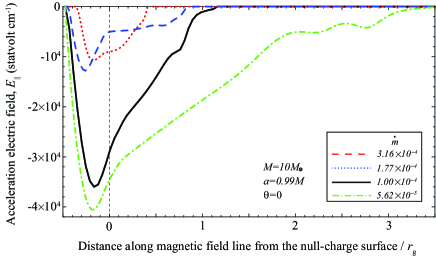
Figure 1: Acceleration electric field, $E_{\parallel}(s)$, along the rotation axis, $\theta=0$, where $s$ denotes the distance (in Boyer-Lindquist radial coordinate) from the null-charge surface along the poloidal magnetic field line. The created current density is 70% of the Goldreich-Julian value, and the injected currents are set to be zero. The red dashed, blue dotted, green dash-dotted, and black solid curves corresponds to $\dot{m}\equiv\dot{M}/\dot{M}_{\rm Edd}=3.16\times 10^{-4}$, $1.77\times 10^{-4}$, $1.00\times 10^{-4}$, and $5.62\times 10^{-5}$, respectively. The vertical dashed line shows the position of the null-charge surface.

5.2 Ultra-relativistic leptons

We next consider the electrons’ distribution function. Because of the the negative $E_{\parallel}$, electrons and positrons are accelerated outward and inward, respectively. As figure 2 shows, the electrons’ Lorentz factors concentrate around $3\times 10^{6}$ due to the curvature-radiation drag. At the same time, electrons distribute at lower Lorentz factors with a broad plateau typically between $6\times 10^{4}$ and $2\times 10^{6}$. Electrons stay at such relatively lower Lorentz factors because of the inverse-Compton drag. Since the Klein-Nishina cross section increases with decreasing Lorentz factors, such lower-energy electrons with $6\times 10^{4}<\gamma<2\times 10^{6}$ efficiently contribute to the VHE emission via the inverse-Compton scatterings.

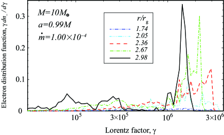
Figure 2: Distribution function of the outwardly propagating electrons at five discrete positions for the same BH parameters as figures. 1. Electron Lorentz factors are saturated around $3\times 10^{6}$ because of the curvature radiation drag. Electrons also distribute in the Lorentz factors below $(1.3\sim 2)\times 10^{6}$ because of the inverse-Compton radiation drag in the deep Klein-Nishina regime.

5.3 Gamma-ray spectra

Let us examine the gamma-ray spectra. In figure 3, we present the Spectral energy distribution (SED) of the gap emission along five discrete viewing angles. It follows that the gap luminosity maximizes if we observe the BH almost face-on, $\theta<15^{\circ}$, and that the gap luminosity rapidly decreases at $\theta<30^{\circ}$ if the gap equatorial boundary is located at $\theta=60^{\circ}$. In what follows, to estimate the maximally possible VHE flux, we consider the emission along the rotation axis, $\theta=0^{\circ}$.

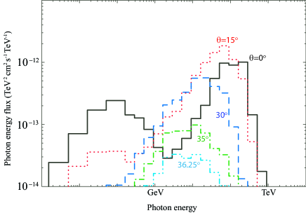
Figure 3: Spectral energy distribution (SED) of the gap-emitted photons along five discrete viewing angles with respect to the rotation axis, $\theta=0^{\circ}$ (black solid line), $\theta=15^{\circ}$ (red dotted), $\theta=30^{\circ}$ (blue dashed), $\theta=35^{\circ}$ (green dash-dotted), and $\theta=36.25^{\circ}$ (cyan dash-dot-dot-dotted). The BH mass and spin are chosen to be $M=10M_{\odot}$ and $a=0.99M$, and the accretion rate is $\dot{m}=1.00\times 10^{-4}$.

We also consider how the the SED depends on the BH spin. In figure 4, we show the SEDs for $a=0.99M$, $0.90M$, and $0.50M$; in each panel, SEDs for the four discrete accretion rates, $\dot{m}=10^{-3.50}$, $10^{-3.75}$, $10^{-4.00}$, and $10^{-4.25}$, are plotted. It is clear that the gap luminosity increases with decreasing $\dot{m}$. It also follows that the gap emission could be detectable with CTA if $a>0.90M$, provided that the distance is within 1 kpc and we observe nearly face on. However, if the BH is moderately rotating as $a=0.50M$, it is very difficult to detect its emission, unless it is located within 0.3 kpc.

In figure 5, we depict the individual emission components, selecting the case of $\dot{m}=10^{-4.00}$. We find that the primary curvature component (magenta dashed line) dominates between 5 MeV and 0.5 GeV, while the primary IC component (magenta dash-dotted line) does above 5 GeV. The secondary IC component (blue dash-dot-dot-dotted line) appears between 0.5 GeV and 5 GeV. The primary IC component suffers absorption above 0.1 TeV.

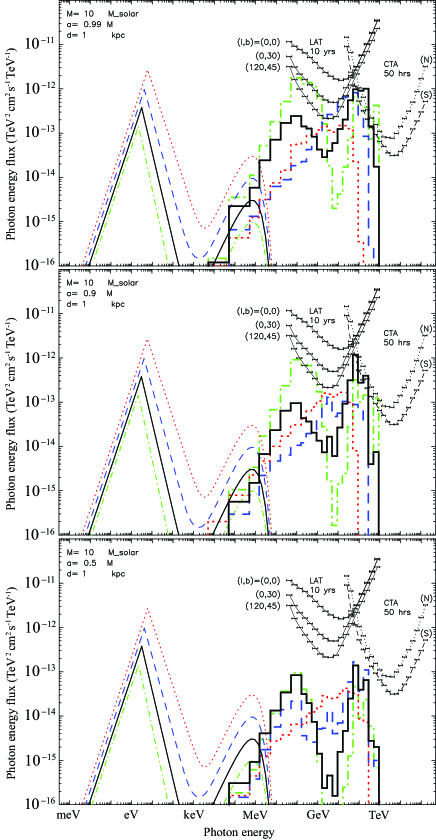
Figure 4: SED of the gap-emitted photons along the rotation axis, $\theta=0^{\circ}$, for $M=10M_{\odot}$. The top panel shows the SED for $a=0.99M$, while the middle and bottom ones for $a=0.90M$ and $a=0.50M$, respectively. The created current density is 70% of the Goldreich-Julian value, and the injected currents are set to be zero. The four thin curves in the left part of each panel show the ADAF emission for $\dot{m}=3.16\times 10^{-4}$ (red dotted), $1.77\times 10^{-4}$ (blue dashed), $1.00\times 10^{-4}$ (black solid), and $5.62\times 10^{-5}$ (green dash-dotted). The four thick curves in the right show the BH gap emission for the corresponding $\dot{m}$.

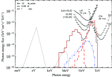
Figure 5: Similar to the top panel of figure 4, but the individual emission components are shown; $\dot{m}=10^{-4}$ is adopted. The black solid line represents the same spectrum as the black solid line in the top panel of figure 4. The magenta dashed line shows the primary curvature component, while the magenta dash-dotted line shows the primary inverse-Compton component. The blue dash-dot-dot-dotted line shows the sum of the synchrotron and inverse-Compton components emitted by the secondary pairs. The thin dotted line shows the input ADAF spectrum.

5.4 Dependence on the created current

Let us demonstrate that the gap solution exists in a wide range of the created electric current within the gap, $j_{\rm cr}\equiv J_{\rm cr}/J_{\rm GJ}$, and that the resultant gamma-ray spectrum little depends on $j_{\rm cr}$. In figure 6, we show the solved $E_{\parallel}(s)$ (left panels) and SEDs (right panels) for three discrete $j_{\rm cr}$’s: from the top, they corresponds to $j_{\rm cr}=0.3$, $0.5$, and $0.9$. The case of $j_{\rm cr}=0.7$ is presented as figure 1 and the top panel of figure 4. It is clear that the gap spectra modestly depends on the created current within the gap as long as the created current is sub-GJ. Note that there exists no stationary gap solutions if the created current density is set to be super-GJ, $j_{\rm cr}>1$.

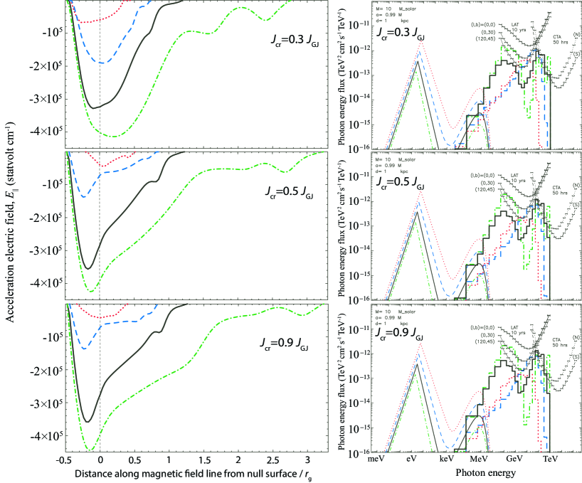
Figure 6: Dependence of the magnetic-field-aligned electric fields $E_{\parallel}(s)$ (left panels) and the SEDs (right panels) on the created current within the gap. From the top, the created current density is 30%, 50%, and 90% of the GJ value. In all the three cases, the injected current density across the inner or outer boundaries are set to be zero. The curves corresponds to the accretion rate of $\dot{m}=3.16\times 10^{-4}$ (red dotted), $1.77\times 10^{-4}$ (blue dashed), $1.00\times 10^{-4}$ (black solid), and $5.62\times 10^{-5}$ (green dash-dotted).

5.5 Dependence on the injected current

The gap solution exists in a wide range of the injected electric currents across the inner and outer boundaries. In this section, we consider only the current injected across the outer boundary, because the positrons created below the separation surface (fig. 2 of Hirotani & Pu (2016), hereafter HP16) may enter the gap across the outer boundary, whereas the electrons created below the inner boundary will fall onto the horizon. In the left panels of figure 7, $E_{\parallel}$ is plotted as a function of the Boyer-Lindquist radial coordinate from the null-charge surface. The red dotted, blue dashed, black solid, and green dash-dotted curves corresponds to the cases of $\dot{m}=10^{-3.50}$, $10^{-3.75}$, $10^{-4.00}$, and $10^{-4.25}$, respectively. From the top, each panel show the results for $j_{\rm out}=0.2$, $0.4$, $0.6$, and $0.8$. In the right panels, SEDs are presented for the same set of $j_{\rm out}$ values. The case of $j_{\rm out}=0$ is presented as figure 1 and the top panel of figure 4.

It follows from the left panels that $E_{\parallel}$ shifts inwards with increasing $J_{\rm out}$ and that $|E_{\parallel}|$ increases as the gap position shifts inwards, as suggested by the outer-gap solutions for rotation-powered pulsars (Hirotani & Shibata, 2001a, b, 2002). Note that the photon-photon collision mean-free path does not decrease as the gap approaches the horizon, which forms a striking contract from pulsars. As a result, the potential drop also increases as the gap shifts inwards in the case of BHs. (In the case of pulsars, the soft photons are emitted from the cooling neutron star surface. Thus, as the gap approaches the stellar surface, the head-on collisions of inward $\gamma$-rays and the outward surface X-rays become more efficient, decreasing the gap longitudinal size and hence the potential drop.) In the present BH cases, the increased $|E_{\parallel}|$ and the potential drop leads to an increased gap luminosity and photon energies in the local reference frame. However, due to the gravitational redshift, the photon energy reduces for a distance static observer. Accordingly, as the right panels show, the final SEDs little change if $j_{\rm out}$ changes from $0$ (top panel of fig. 4) to $0.8$ (bottom right panel of this fig. 7), although the $E_{\parallel}(s)$ distribution changes significantly as figure 1 and left panels of figure 7 show.

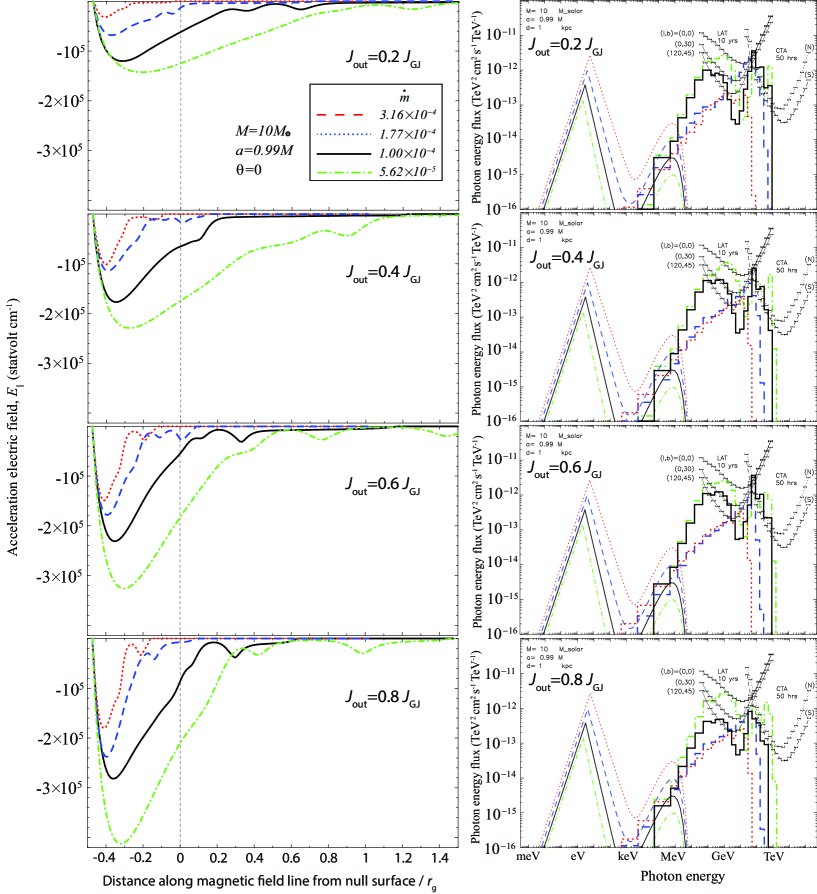
Figure 7: Dependence of the magnetic-field-aligned electric fields $E_{\parallel}(s)$ (left panels) and the SEDs (right panels) on the injected positronic current across the outer boundary. From the top, the injected current density is 20%, 40%, 60%, and 80% of the GJ value. In all the four cases, the created current density within the gap is fixed to be 70% of the GJ value, and the injected electronic current across the inner boundary are set to be zero. The curves corresponds to the accretion rate of $\dot{m}=3.16\times 10^{-4}$ (red dotted), $1.77\times 10^{-4}$ (blue dashed), $1.00\times 10^{-4}$ (black solid), and $5.62\times 10^{-5}$ (green dash-dotted). Note that the ordinate scale is ten times greater than figure 1

6 Discussion

To sum up, we examined stationary solutions of the electron-positron accelerator exerted in a rotating BH magnetosphere. Depending on the molecular hydrogen density and the BH velocity with respect to the molecular cloud, the Bondi accretion rate can be adjusted as $6\times 10^{-5}<\dot{m}<10^{-4}$ in the Eddington unit. In this case, $\gamma$-rays are efficiently emitted outward in the polar region, typically $\theta\leq 15^{\circ}$, and the emission from a stellar-mass BH could be marginally detectable with CTA, provided that the BH is rapidly rotating (e.g., $a>0.9M$), and that the accretion rate is adjusted in the range $6\times 10^{-5}<\dot{m}<10^{-4}$. The final photon spectrum little depends on the created current density within the gap, or on the externally injected current density across the outer boundary.

6.1 Comparison with other gamma-ray emission models from molecular clouds

We compare the gamma-ray emission scenarios from molecular clouds (table 1). In the protostellar jet scenario (Bosch-Ramon et al., 2010), jets are ejected from massive protostars to interact with the surrounding dense molecular clouds, leading to an acceleration of electrons and protons at the termination shocks. Accordingly, the size of the emission region becomes comparable to the jet transverse thickness at the shock. In the hadronic cosmic ray scenario (Ginzburg & Syrovatskii, 1964; Blandford & Eichler, 1987), protons and helium nuclei are accelerated in the supernova shock fronts, a portion of which propagate into dense molecular clouds. As a result of the proton-proton (or nuclear) collisions, neutral pions are produced and decay into gamma-rays, whose spectrum becomes a single power-law between 0.001-100 TeV. Since this interaction takes place most efficiently in a dense gaseous region, the size of the gamma-ray image will become comparable to the core of a dense molecular cloud. In the leptonic cosmic ray scenario (Aharonian et al., 1997; van der Swaluw et al., 2001; Hillas et al., 1998), electrons are accelerated at pulsar wind nebulae or shell-type supernova remnants, and radiate radio/X-rays and gamma-rays via synchrotron and IC processes, respectively. Since the cosmic microwave background radiation provides the main soft photon field in the interstellar medium, the size may be comparable to the plerions, whose size increases with the pulsar age. In the BH-gap scenario (see § 1 for references), emission size does not exceed $10r_{\rm g}$. Since the angular resolution of the CTA is about five times better than the current IACTs, we propose that we can discriminate the present BH-gap scenario from the three above-mentioned scenarios by comparing the gamma-ray image and spectral properties. Namely, if a VHE source has a point-like morphology like HESS J1800-2400C in a gaseous cloud (§ 2), and if the spectrum has two peaks around 0.01–1 GeV and 0.01–1 TeV, but shows (synchrotron) power-law component in neither radio nor X-ray wavelengths, we consider that the present scenario accounts for its emission mechanism.

Table 1: Gamma-ray emission models from molecular clouds^a.

Model	Emission processes (spectral shape; energy range)	Size (cm)
Protostellar jets	$e^{-}$ synchrotron (power-law; $10^{-6}$ eV–$10^{2}$ eV);	$10^{16}$–$10^{17}$
	$e^{-}$ Bremsstrahlung (power-law; 0.1 MeV–TeV);
	$pp$ collisions, $\pi^{0}$ decaysb (power-law; GeV–TeV)
Cosmic ray hadrons	$pp$ collisions, $\pi^{0}$ decaysb (power-law; GeV–100 TeV)	$10^{18}$–$10^{19}$
Cosmic ray leptonsc	$e^{-}$ synchrotron (power-law; $10^{-6}$ eV–$10^{2}$ eV);	$10^{18}$–$10^{20}$
	$e^{-}$ IC scatterings (broad peak; GeV–10 TeV)
BH gap	$e^{-}$ curvature process (broad peak; 0.01 GeV–1 GeV);	$10^{7}$
	$e^{-}$ IC scatterings (sharp peak; around 0.1 TeV)

6.2 Current injection and time dependence

Although the magnetic (i.e., one-photon) pair production is also taken into account, most electron-positron pairs are found to be produced via photon-photon (i.e., two-photon) collisions, which take place via two paths. One path is through the collisions of the two MeV photons both of which were emitted from the equatorial ADAF. Another path is through the collisions of TeV and eV photons; the former photons were emitted by the gap-accelerated leptons via inverse-Compton process, while the latter were emitted from the ADAF via synchrotron process. There is, indeed, the third path, in which the gap-emitted GeV curvature photons collide with the ADAF-emitted keV inverse-Compton photons; however, this path is negligible particularly when $\dot{m}\ll 1$. If the pairs are produced via TeV-eV collisions (i.e., via the second path) outside the gap outer boundary, they have outward ultra-relativistic momenta to easily ‘climb up the hill’ of the potential $k_{0}$ (see fig. 2 of HP16) and propagate to large distances without turning back. However, if the pairs are produced via MeV-MeV collisions (i.e., via the first path), they are produced with sub-relativistic outward momenta; thus, they eventually return to fall onto the horizon due to the strong gravitational pull inside the separation surface (fig. 2 of HP16). When the returned pairs arrive the gap outer boundary, only positrons can penetrate into the gap because of $E_{\parallel}<0$. Accordingly, electrons accumulate at the boundary, whose surface charge leads to the jump of the normal derivative of $E_{\parallel}$. Thus, although the stationary gap solutions show that the $\gamma$-ray spectrum little depends on the injected current density (§ 5.5), the gap solution inevitably becomes time-dependent due to the increasing discontinuity of $|dE_{\parallel}/dr|$ with an accumulated surface charge (in this case, electrons) at the outer boundary. If the injected current is much small compared to the GJ current, the time dependence will be mild. However, if the injected current becomes a good fraction of the GJ current, the assumption of the stationarity becomes invalid, as pointed out by Levinson & Segev (2017). In this sense, a caution should be made in the applicability of the stationary solutions presented in this paper, when the injected current is non-negligible compared to the current created within the gap.

6.3 Stability of stationary black hole gaps

In this subsection, we consider the stability of our stationary gap solutions. In the case of pulsar polar caps, it has been revealed that the pair production cascade takes place in a highly time-dependent way by particle-in-cell (PIC) simulations (Timokhin & Arons, 2013; Timokhin & Harding, 2015; Timokhin, 2010). Moreover, in the case of BH magnetospheres, it is recently demonstrated that a gap exhibits rapid spatial and temporal oscillations of the magnetic-field-aligned electric field and current by 1-D PIC simulations (Levinson & Segev, 2017; cheng18). It is, however, out of the scope of the present paper to perform a PIC simulation or a linear perturbation analysis to examine the stability of a stationary gap solution. Instead, we will qualitatively discuss why we seek stationary solutions, comparing with pulsar outer-magnetospheric and polar-cap gaps.

We start with discussing the pulsar outer (-magnetospheric) gaps, because they have essentially the same electrodynamics as BH gaps. Since the neutron star’s dipole magnetic field lines have convex geometry, the magnetic field becomes perpendicular with respect to the star’s rotation axis at a good fraction of the so-called “light cylinder radius.” In this case, if the magnetosphere is highly vacuum in the sense $|\rho|\ll|\rho_{\rm GJ}|$ in equation (8), $\rho-\rho_{\rm GJ}\approx-\rho_{\rm GJ}>0$ (or $<0$) holds in the lower (or the upper) half of the gap. As a result, $E_{\parallel}$ has a positive (or negative) gradient in the lower (or the upper) half; thus, the acceleration electric field naturally closes. Note that $E_{\parallel}>0$ is realized when the magnetic axis resides in the same hemisphere as the rotation axis. Without loss of any generality, we can adopt such a positive $E_{\parallel}$ in the outer-gap model.

Because $E_{\parallel}>0$, positrons (or electrons) are accelerated outwards (or inwards). Thus, $\rho$ has a positive gradient along individual magnetic field lines. When the gap closure condition is satisfied, there exists a stationary solution whose $\rho/B$ distribution can be illustrated as the left panel of figure 8. If pair production increases perturbatively from this stationary solution, $\rho-\rho_{\rm GJ}$ decreases its absolute value, which leads to an decrease of $E_{\parallel}$ due to the reduced gradient of $|\rho-\rho_{\rm GJ}|$, and hence an decrease of the pair production (right panel of fig. 8). Note that this negative feedback effect works because of $E_{\parallel}>0$, which stems from the fact that there exists a null-charge surface in the gap. As a result, the outer gap solutions exist for a wide range of pulsar parameters such as the period, period derivative, neutron-star surface temperature, inclination of the magnetic axis with respect to the star’s rotation axis, as well as the magnetospheric current, from young, middle-aged to millisecond pulsars. Analogous (but still qualitative) argument of gap stability is possible if we use the gap closure condition; see section 5.2 of Hirotani (2001) for details.

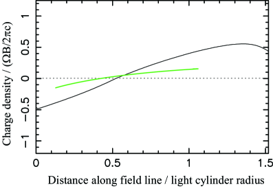
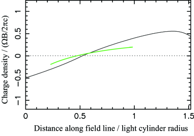
Figure 8: Schematic picture of the distribution of a dimensionless charge density per magnetic flux tube, $(2\pi/\Omega_{\rm F})(\rho/B)$, in the pulsar outer-gap model. A positive acceleration electric field, $E_{\parallel}$, arises, because $\rho-\rho_{\rm GJ}>0$ holds (i.e., $dE_{\parallel}/ds>0$), in the inner part of the gap, and because $\rho-\rho_{\rm GJ}<0$ holds (i.e., $dE_{\parallel}/ds<0$) in the outer part. The dimensionless Goldreich-Julian charge density, $(2\pi/\Omega_{\rm F})(\rho_{\rm GJ}/B)$ is depicted by the solid curve. Left: As an initial state, we consider a typical $\rho/B$ distribution (green solid curve) of a non-vacuum outer gap. Created positrons (or electrons) are accelerated outwards (or inwards) by the positive $E_{\parallel}$; therefore, $\rho/B$ has a positive gradient. Right: Imagine that the pair production increases perturbatively. Because $E_{\parallel}>0$, created and migrated positrons (or electrons) increase (or decrease) $\rho$ at the outer (or inner) part of the gap. As a result, the reduced $\rho-\rho_{\rm GJ}$ partly cancels the original $E_{\parallel}$, reducing the perturbatively increased pair production. Because of this negative feedback effect, the outer-gap solution depends on the pulsar parameters, as well as the magnetospheric current, only modestly (Hirotani, 2001).

Because null-charge surfaces also exist around rotating BHs, the gap electrodynamics little changes between pulsar outer gaps and BH gaps. Around a rotating BH, a null surface is formed near the event horizon by the frame-dragging. However, around a rotating neutron star, it is formed in the outer magnetosphere (i.e., far away from the neutron star) by the convex magnetic-field geometry. Accordingly, a negative feedback effect also works in BH gaps. That is, the gap closure condition, which is required for a BH gap to be stationary, is accommodated for a wide range of magnetospheric current values, as explicitly demonstrated in § 5.

Since there frequently appears a confusion between pulsar polar-cap and outer-gap (and hence BH-gap) electrodynamics, particularly on the stability argument, it is helpful to describe also the pulsar polar-cap accelerator. In a pulsar polar cap, there exists no null surface. Thus, if a three-dimensional polar cap region is charge starved in the sense $|\rho-\rho_{\rm GJ}|\ll\rho_{\rm GJ}$, a positive $-\rho_{\rm GJ}$ leads to a negative $E_{\parallel}$ when the magnetic axis resides in the same hemisphere as the rotation axis. Accordingly, electrons are drawn from the neutron star surface as a space-charge-limited flow. In the direct vicinity of the neutron star surface, the non-relativistic electrons produces a large negative $\rho$ (the green vertical lines along the ordinates in figure 9) such that $\rho-\rho_{\rm GJ}\approx\rho<0$. In the outer part of a polar cap accelerator, on the other hand, relativistic electrons produces a moderate negative charge density such that $\rho-\rho_{\rm GJ}>0$ (left panel of fig. 9). Thus, $E_{\parallel}$ has a negative gradient along the magnetic field in the direct vicinity of the neutron star, but it has a positive gradient near the upper boundary where $\rho-\rho_{\rm GJ}\approx 0$. Accordingly, we obtain a negative $E_{\parallel}$ in the pulsar polar caps.

However, if a small-amplitude pair production takes place in the polar gap, inwardly migrating positrons (or outwardly migrating electrons) result in an increased (or decreased) $\rho-\rho_{\rm GJ}$ in the lower (or the upper) half of the gap (right panel of fig. 9). Accordingly, $|E_{\parallel}|$ increases (or decreases) in the lower part (or the upper-most part). The increased $|E_{\parallel}|$ further enhances pair production in the upper-most part, and $|E_{\parallel}|$, and hence the pair production increases with time. Because of this positive feedback effect, instability sets in, as demonstrated by PIC simulations (Timokhin & Arons, 2013; Timokhin, 2010). In short, pulsar polar cap accelerators are inherently unstable for pair production because of $E_{\parallel}<0$, which stems from the fact that there exists no null-charge surface in the pulsar polar-cap region.

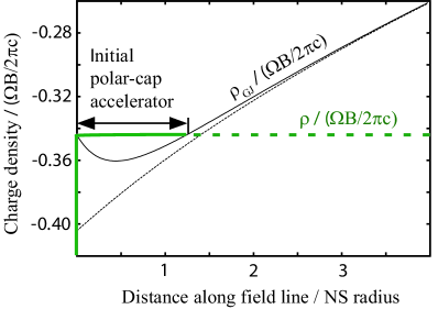
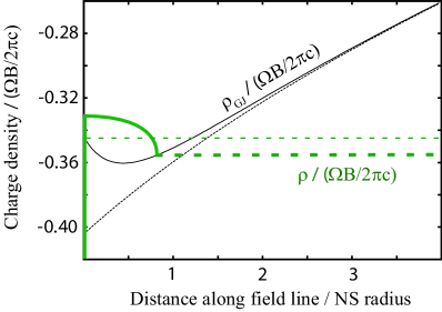
Figure 9: Schematic picture of the distribution of a $\rho/B$ in the pulsar polar-cap model. A negative $E_{\parallel}$ arises, because $\rho-\rho_{\rm GJ}>0$ holds in the entire gap except for the direct vicinity of the neutron star surface. This negative $E_{\parallel}$ extract electrons from the stellar surface as a space-charge-limited flow. The dimensionless Goldreich-Julian charge density, $\rho_{\rm GJ}/B$ is depicted by the solid curve, while its Newtonian value is plotted by the thin black dotted curve. Left: As an initial state, we consider no pair production; thus, $\rho/B$ tends to a constant value, as the horizontal green line shows. The polar-cap accelerator (i.e., gap) arises approximately within the region where $\rho>\rho_{\rm GJ}$ holds above the stellar surface. Right: The outwardly accelerated electrons emit the $\gamma$-rays that materialize as pairs in the upper-most part of the gap. The separated electrons move outwards reducing $\rho$ from its initial value, while positrons move inwards increasing $\rho$. Accordingly, in the lower part of the initial gap, increased $E_{\parallel}$ leads to a further enhanced pair production; this positive feedback effect results in an instability (Timokhin & Arons, 2013).

On these grounds, we cannot readily conclude that the stationary BH gap solutions presented in this paper are unstable because of the highly time-dependent nature of pulsar polar gaps. A careful examination with a PIC simulation is needed for BH gaps, as performed recently by Levinson & Segev (2017). Since the saturated solution given by Levinson & Segev (2017) is much less violently time-dependent compared to pulsar polar-cap accelerators (Timokhin & Arons, 2013), we have sought stationary solutions of BH gaps as the first step in the present paper.

References

- Aharonian et al. (1997) Aharonian, F. A. Atoyan, A. M. Kifune, T. 1997, MNRAS, 291, 162
- Aharonian et al. (2006) F. Aharonian, A. G. Akhperjanian, A. R. Bazer-Bachi, M. Beilicke, W. Benbow, D. Berge, K. Boenlöhr, C. Boisson et al. 2006, ApJ, 636, 777 (2006)
- Aharonian et al. (2008a) F. Aharonian, A. G. Akhperjanian, A. R. Bazer-Bachi, B. Behera, M. Beilicke, W. Benbow, D. Berge, K. Boenlöhr, C. Boisson et al. 2008a, A&A, 481, 401 (2008a)
- Aharonian et al. (2008b) F. Aharonian, A. G. Akhperjanian, U. Barres de Almeida, A. R. Bazer-Bachi, B. Behera, M. Beilicke, W. Benbow, K. Boenlöhr, C. Boisson et al. 2008b, A&A, 483, 509 (2008b)
- Aharonian et al. (2008c) F. Aharonian, A. G. Akhperjanian, U. Barres de Almeida, A. R. Bazer-Bachi, B. Behera, M. Beilicke, W. Benbow, K. Boenlöhr, C. Boisson et al. 2008c, A&A, 490, 685 (2008c)
- Aharonian et al. (2008d) F. Aharonian, A. G. Akhperjanian, U. Barres de Almeida, A. R. Bazer-Bachi, B. Behera, M. Beilicke, W. Benbow, K. Boenlöhr, C. Boisson et al. 2008d, A&A, 477, 353 (2008d)
- Abramowski et al. (2014) A. Abramowski, F. Aharonian, F. Ait Benkhali, A. G. Akhperjanian, E. O. Angüner, M. Backes, S. Balenderan, A. Balzer, A. Barnacka et al. 2014, ApJ, 794, L1 (2014)
- Beskin et al. (1992) Beskin, V. S., Istomin, Ya. N., & Par’ev, V. I. 1992, Sov. Astron., 36(6), 642
- Blandford & Eichler (1987) Blandford, R. D. , Eichler, D. 1987, Phys. Rep., 154, 1
- Blitz (1980) L. Blitz, Large scale mapping of local molecular cloud complexes, in Giant Molecular Cluds in the Galaxy ed. P. M. Solomon, M. G. Edmunds, 1980, Pergamon Press, pp. 1–18
- Bondi & Hoyle (1944) Bondi, H., Hoyle, F. 1944, MNRAS, 104, 273
- Bosch-Ramon et al. (2010) Bosch-Ramon, G. E. Romero, A. T. Araudo, J. M. Paredes, 2010, A&A, 511, 8
- Boyer & Lindquist (1967) Boyer, R. H. & Lindquist, R. W. 1967 J. Math. Phys., 265, 281
- Broderick & Tchekhovskoy (2015) Broderick, A. E., Tchekhovskoy A. 2015, ApJ, 809, 97
- Cheng et al. (1986a) Cheng, K. S., Ho, C. & Ruderman, M. 1986a, ApJ, 300, 500
- Cheng et al. (1986b) Cheng, K. S., Ho, C. & Ruderman, M. 1986b, ApJ, 300, 522
- Cheng et al. (2000) Cheng, K. S., Ruderman, M. & Zhang, L. 2000, ApJ, 537, 964
- Chen et al. (2018) Chen, A. Y., Yuan Y., & Yang, H. 2018, arXiv:1805.11039v1
- Chiang & Romani (1992) Chiang, J. & Romani, R. W. 1992, ApJ, 400, 629
- Daugherty & Harding (1982) Daugherty, J. K. & Harding, A. K. 1982, ApJ, 252, 337
- de Wilt et al. (2017) P. de Wilt, G. Rowell, A. J. Walsh, M. Burton, J. Rathborne, Y. Fukui, A. Kawamura, F. Aharonian, 2017, MNRAS, 468, 2093
- Dermer (1994) Dermer, C. D. & Sturner, S. J. 1994, ApJ, 420, L75
- Ginzburg & Syrovatskii (1964) V. L. Ginzburg, S. I. Syrovatskii, 1964, 18. The Origin of Cosmic Rays (New York; Maccmillan)
- Globus & Levinson (2014) N. Globus, A. Levinson, 2014, ApJ, 796, 26
- Goldreich & Julian (1969) Goldreich, P., Julian, W. H., 1969, ApJ, 157, 869
- Harding et al. (1978) Harding, A. K., Tademaru, E. & Esposito, L. S. 1978, ApJ, 225, 226
- Harding (1981) Harding, A. K. 1981, ApJ, 245, 267
- Hillas et al. (1998) A. M. Hillas, C. W. Akerlof, S. D. Biller , J. H. Buckley, D. A. Carter-Lewis, M. Catanese, M. F. Cawley, D. J. Fegan, J. P. Finley, J. A. Gaidos, F. Krennrich, R. C. Lamb, M. J. Lang, G. Mohanty, M. Punch, P. T. Reynolds, A. J. Rodgers, H. J. Rose, A. C. Rovero, M. S. Schubnell, G. H. Sembroski, G. Vacanti, T. C. Weekes, M. West, J. Zweerink, 1998, ApJ, 503, 744 (1998).
- Hirotani & Okamoto (1998) Hirotani, K. & Okamoto, I. 1998, ApJ, 497, 563
- Hirotani & Shibata (1999) Hirotani, K., & Shibata, S. 1999, MNRAS, 308, 54
- Hirotani (2001) K. Hirotani, 2001, ApJ, 549, 495
- Hirotani & Shibata (2001a) Hirotani, K., & Shibata, S. 2001, ApJ, 558, 216
- Hirotani & Shibata (2001b) Hirotani, K., & Shibata, S. 2001, MNRAS, 325, 1228
- Hirotani & Shibata (2002) Hirotani, K., & Shibata, S. 2002, ApJ, 564, 369
- Hirotani et al. (2003) Hirotani, K., Harding, A. K., & Shibata, S., 2003, ApJ, 591, 334
- Hirotani (2006) Hirotani, K. 2006, Mod. Phys. Lett. A (Brief Review), 21, 1319
- Hirotani (2013) Hirotani, K. 2013, ApJ, 766, 98
- Hirotani & Pu (2016) Hirotani, K., Pu, H.-Y. 2016, ApJ, 818, 50 (HP16)
- Hirotani et al. (2016b) Hirotani, K. Pu, H.-Y. Lin, L. C.-C. Chang, H.-K. Inoue, M. Kong, A. K. H. Matsushita, S. Tam, P.-H. T. 2016, ApJ, 833, 142
- Hirotani et al. (2017) Hirotani, K. Pu, H.-Y. Lin, L. C.-C., Kong, A. K. H. Matsushita, S. Asada, K. Chang, H.-K. Tam, P.-H. T. 2017, ApJ, 845, 77
- Hirotani et al. (2018) Hirotani, K. Pu, H.-Y. Matsushita, S. 2018, J. Astrophys. Astr. 39, 50
- Hofverberg et al. (2010) Hofverberg, P. Chaves, R. C. G. Fiasson, A. Kosack, K. Méhault, J. de Onã Wilhelmi E. for the H. E. S. S. Collaboration Proc. Sci., Discovery of VHE gamma-rays from the vinicity of the shell-type SNR G318.2+0.1 with H. E. S. S. SISSA, Trieste, PoS, 2010, Texas 2010, 196
- Kerr (1963) Kerr, R. P. 1963, Phys. Rev. Lett., 11, 237
- Komissarov & McKinney (2007) Komissarov, S. S. McKinney, J. C. 2007, MNRAS, 377, L49
- Levinson & Rieger (2011) Levinson, A., Rieger, F. 2011, ApJ, 730, 123
- Lin et al. (2017) Lin, L. C.-C. Pu, H.-Y. Hirotani, K. Kong, A. K. H. Matsushita, S. Chang, H.-K. Inoue, M. Tam, P.-H. T. 2017, ApJ, 845, 40
- Levinson & Segev (2017) A. Levinson, N. Segev, 2017, PRD 96, id.123006
- Mahadevan (1997) Mahadevan, R. 1997, ApJ, 477, 585
- Mestel (1971) Mestel L., 1971, Nature, 233, 149
- Narayan & Yi (1994) Narayan, R., Yi, I., 1994, ApJ, 428, L13
- Narayan & Yi (1995) Narayan, R., Yi, I., 1995, ApJ, 452, 710
- Neronov & Aharonian (2007) Neronov, A., Aharonian, F. A. 2007, ApJ, 671, 85
- Rieger & Aharonian (2008) Rieger, F. M., Aharonian, F. A. A&A, 479, L5
- Romani (1996) Romani, R. 1996, ApJ, 470, 469
- Sitnik (2003) Sitnik, T. G. 2003, Astron. Lett. 29, 356
- Song et al. (2017) Song, Y. Pu, H.-Y. Hirotani, K. Matsushita, S. Kong, A. K. H. Chang, H.-K. 2017, MNRAS, 471, L135
- Takahashi et al. (1990) Takahashi, M., Nitta, S., Tatematsu, Y., Tomimatsu, A. 1990, ApJ, 363, 206
- Timokhin (2010) Timokhin, A. N., 2010, MNRAS, 408, 2092
- Timokhin & Arons (2013) Timokhin, A. N., Arons, J., 2013, MNRAS, 429, 20
- Timokhin & Harding (2015) Timokhin, A. N., Harding, A. K., 2015, ApJ, 810, 144
- Tchekhovskoy et al. (2010) Tchekhovskoy, A., Narayan, R., McKinney, J. C. 2010, ApJ, 711, 50
- van der Swaluw et al. (2001) van der Swaluw, E. , Achterberg, A. Gallant, Y. A. Toth, G. 2001, A&A, 380, 309 (2001).