Disorder-safe entanglement transfer through ladder qubit chains

Abstract

We study an entanglement transfer protocol in a two-leg ladder spin-1/2 chain in the presence of disorder. In the regime where on-site energies and the intrachain couplings follow aproximately constant proportions locally, we set up a scheme for high-fidelity state transfer via a disorder-protected subspace wherein fluctuations in the parameters do not depend on the global disorder of the system, accounted by $W$. Moreover, we find that the leakage of information from that subspace is actually suppressed upon increasing $W$ and thus the transfer fidelity, evaluated through the entanglement concurrence at the other end of the chain, builds up with the disorder strength.

I Introduction

In the past decade, 1D spin chains have been regarded as potential quantum communication platforms for a wide variety of tasks (see Apollaro et al. (2013); Nikolopoulos and Jex (2014) and references within). In standard quantum-state transfer protocols Bose (2003), for instance, the chain must be manufactured in such a way an arbitrary qubit can be faithfully sent from one point to another at some (preferably small) prescribed time following the natural underlying Hamiltonian dynamics of the system.

To do so, a handful of schemes have have been put forward since the original proposal in Ref. Bose (2003), some relying on fully-engineered couplings Christandl et al. (2004); Plenio et al. (2004); Nikolopoulos et al. (2004) – thereby yielding perfect transfer through arbitrary distances –, dual-rail encoding Burgarth and Bose (2005), strong local magnetic fields Lorenzo et al. (2013, 2015), and weak-end couplings Wójcik et al. (2005); *wojcik07; Li et al. (2005); Almeida et al. (2016); Almeida (2018) to name a few.

Given the possibility of experimental errors in the manufacturing process of the chain and that one is willing not to interfere with the channel while it is operating in order to avoid decoherence and losses, disorder stands out as a major threat to the performance of the protocol. This fact alone has motivated several studies on the influence of static fluctuations in the parameters of the chain over the state transfer fidelity Allcock and Linden (2009); De Chiara et al. (2005); Fitzsimons and Twamley (2005); Burgarth and Bose (2005); Tsomokos et al. (2007); Petrosyan et al. (2010); Yao et al. (2011); Zwick et al. (2011); *zwick12; Bruderer et al. (2012); Kay (2016); Almeida et al. (2017, 2018a, 2018b).

It is pretty well established that 1D and 2D single-particle hopping models display Anderson localization for any degree of uncorrelated disorder Anderson (1958); *abrahams79. A very rich cross-over between localization and delocalization, though, can be found in chains displaying certain kinds of correlated disorder Dunlap et al. (1990); *phillips91; de Moura and Lyra (1998); Izrailev and Krokhin (1999); Kuhl et al. (2000); Izrailev et al. (2012). For instance, it was shown in de Moura and Lyra (1998) that long-range correlated disorder induces the appearance of a band of extended states with sharp mobility edges thereby indicating a metal-insulator transition. Very recently, we have explored this breakdown of Anderson localization in order to carry out quantum-state transfer protocols Almeida et al. (2017, 2018a, 2018b). Another kind of configuration that deserves attention is quasi-1D models such as ladder networks. In Sil et al. (2008a), it was reported that a two-leg Aubry-André model displays a metal-insulator transition with multiple mobility edges. They also put forward the possibility of spanning a band of disorder-free states coexisting with exponentially-localized modes given the on-site energies and interchain hopping strenghts follow constant proportions along the ladder Sil et al. (2008b). de Moura et al. further found out a novel level- spacing statistics associated to it de Moura et al. (2010). A generalized version of this wavefunction delocalization engineering for $N$-leg ladder systems has also been put forward Rodriguez et al. (2012). The inteplay between channels featuring different degrees and/or types of disorder has also been investigated Zhang et al. (2010); Guo and Xiong (2011).

In this work we bring about the idea of disorder-free subspaces spanning over a strongly disordered media Sil et al. (2008b); Rodriguez et al. (2012) into the context of quantum communication protocols. In particular, we aim to transmit entanglement with high fidelity from one end of a two-leg ladder chain to the other in the presence of disorder. We outline the parameter conditions for which a disorder-free channel arises and how to properly encode the initial entangled state in order to use it. We further consider imperfections in this channel which can promote the leakage of information out of it. Our main result is that this effect can be avoided when we increase the amount of disorder originally present in the system. This remarkable behavior paves the way for disorder-safe quantum communication protocols in engineered qubit chains.

In the following, Sec. II we introduce the Hamiltonian model and in Sec. III we discuss the conditions for setting up a disorder-free channel. In Sec. IV we display our results for the entanglement transfer performance against disorder as well as we investigate the leakage of information out of the protected subspace. Our conclusions are drawn in Sec. V.

II Model and formalism

Here, we deal with a two-leg ladder spin (qubit) chain of the $XX$ type, with $N$ sites each, described in terms of a free-fermion Hamiltonian of the form $H=H^{(1)}+H^{(2)}+H_{I}$, with ($\hbar=1$)

$$H^{(j)} =\sum_{n=1}^{N}\epsilon_{n,j}c_{n,j}^{\dagger}c_{n,j}+\sum_{n=1}^{N-1}J_{n,j}(c_{n+1,j}^{\dagger}c_{n,j}+\mathrm{H.c.}),$$ (1)

$$H_{I} =\sum_{n=1}^{N}\gamma_{n}(c_{n,2}^{\dagger}c_{n,1}+\mathrm{H.c.}),$$ (2)

where $c_{n,j}^{\dagger}$ ($c_{n,j}$) creates (removes) a fermion at the $n$-th site of the $j$-th chain ($j=1,2$), $\epsilon_{n,j}$ stands for its local potential, $J_{n,j}$ is the intra-chain hopping rate, and $\gamma_{n}$ is the inter-chain hopping rate. Throughout this paper we consider $J_{n,1}=J_{n,2}\equiv J_{n}$ and set $J=\mathrm{max}\{J_{n}\}\equiv 1$ as the energy unit. Note that $H$ conserves the total number of excitations. Here we are interested in the single-excitation manifold spanned by

$$|\textbf{n}\rangle^{(j)}\equiv c_{n,j}^{\dagger}\bigotimes_{i=1}^{2}|00\cdots 0\rangle^{(i)},$$ (3)

thereby forming a 2N-dimensional Hilbert space.

We now allow disorder to occur on the on-site potentials $\epsilon_{n,j}$ and inter-chain coupling rates $\gamma_{n}$. In particular, we assume these quantities to fall within a uniform random distribution in the interval $[-W,W]$, $W$ being the intensity of disorder. Further, we consider $J_{n,1}=J_{n,2}\equiv J_{n}$.

In Sil et al. (2008b) (see also de Moura et al. (2010)) it was shown that when $\epsilon_{n,1}$, $\epsilon_{n,2}$, and $\gamma_{n}$ obey constant proportions between each other across the chain, one is able to choose an appropriate basis set that decouples both legs. Moreover, it is possible to turn one of them completely free of disorder Sil et al. (2008b). To see this happening, let us define

$$|\textbf{n},\pm\rangle=\dfrac{|\textbf{n}\rangle^{(1)}\pm|\textbf{n}\rangle^{(2)}}{\sqrt{2}},$$ (4)

and rewrite Hamiltonian $H$ in terms of these states, to get

$$H =\sum_{\mu=\pm}\left[\sum_{n=1}^{N}\widetilde{\epsilon}_{n,\mu}|\textbf{n},\mu\rangle\langle\textbf{n},\mu|+\sum_{n=1}^{N-1}J_{n}(|\textbf{n}+\textbf{1},\mu\rangle\langle\textbf{n},\mu|+\mathrm{H.c.})\right]$$

$$\,\,\,\,\,\,+\sum_{n=1}^{N}\widetilde{\gamma}_{n}(|\textbf{n},+\rangle\langle\textbf{n},-|+\mathrm{H.c.}),$$ (5)

with

$$\widetilde{\epsilon}_{n,\pm} =\dfrac{\epsilon_{n,1}+\epsilon_{n,2}}{2}\pm\gamma_{n},$$ (6)

$$\widetilde{\gamma}_{n} =\dfrac{\epsilon_{n,1}-\epsilon_{n,2}}{2},$$ (7)

being the potentials and inter-chain coupling rates, respectively, for the effective ladder with both legs extending over $|\textbf{n},+\rangle$ and $|\textbf{n},-\rangle$.

III Disorder-free subspace

From Hamiltonian (II), we readily note that setting $\epsilon_{n,1}=\epsilon_{n,2}$ leads to the decoupling of both legs. In addition, when $\epsilon_{n,1}=\gamma_{n}$ then the anti-symmetric branch takes $\widetilde{\epsilon}_{n,-}=0$. The availability of a ordered subspace embedded in a strongly disordered media is very appealing when it comes to, e.g., running pre-engineered quantum-state transfer protocols Bose (2003). Suppose we have an imperfect (single-leg) chain due to uncorrelated on-site fluctuations. By generating another copy of it and linking them up one may find a clean, disorder-free quantum communication channel by properly enconding the qubit [e.g. following Eq. (4)] to be sent through, no matter how strong $W$ is.

A possible issue that might set in, though, is that the second (backup) leg may not be a legit copy of the first one. That would keep disorder in the channel as well as promote the leakage of information from $|\textbf{n},-\rangle$ into $|\textbf{n},+\rangle$. Still, if we allow for small deviations in, say, $\epsilon_{n,2}$ around $\epsilon_{n,1}$, it is possible to keep the channel reasonably safe. For instance, let $\epsilon_{n,2}=\epsilon_{n,1}+\delta_{n}$, with $\delta_{n}$ being another random number, uniformly distributed within $[-\Delta,\Delta]$ such that $\Delta\ll W$. By looking at Eqs. (6) and (7), we now have $\widetilde{\gamma}_{n}=-\delta_{n}/2$ and $\widetilde{\epsilon}_{n,-}=\delta_{n}/2$. Therefore, disorder in leg $\{|\textbf{n},-\rangle\}$ is solely weighted by $\Delta$ and not by $W$, so that the latter can be arbitrarily large. If $\Delta\neq 0$ there will be leakage into $\{|\textbf{n},+\rangle\}$, this subspace now acting as an disordered “environment” with on-site energies given by $\widetilde{\epsilon}_{n,+}=(4\epsilon_{n,1}+\delta_{n})/2$. Note that we are still considering $\gamma_{n}=\epsilon_{n,1}$. Small deviations from it would not affect $\widetilde{\gamma}_{n}$, but the on-site potentials $\widetilde{\epsilon}_{n,+}$ and $\widetilde{\epsilon}_{n,-}$ with a small shift. Because of that, here disorder will be ultimately set by $W$ (global disorder) and $\Delta$ in the regime $\Delta\leq W$ with $\Delta\ll J$.

IV Results and discussion

IV.1 Entanglement transfer

Now, suppose Alice has access to the first “cell” of the ladder and is willing to send some amount of entanglement to Bob at at the other end of the ladder relying only upon the natural Hamiltonian dynamics of the system Bose (2003). In order to make use of the disorder-protected subspace as discussed in the previous section, a bipartite entangled state of the Bell type can be properly prepared in the following way. A single-excitation (spin up) is initially set by Alice in one of her sites of domain $|01\rangle_{A}$. By further applying the Hadamard gate $H_{\mathrm{gate}}$ at her second qubit followed by a CNOT gate controlled by the same one (being $|0\rangle$) she gets

$$|\phi\rangle_{A} =CNOT(I\otimes H_{\mathrm{gate}})|01\rangle_{A}$$

$$=CNOT|0\rangle_{A}\left(\frac{|0\rangle_{A}-|1\rangle_{A}}{\sqrt{2}}\right)$$

$$=\frac{|10\rangle_{A}-|01\rangle_{A}}{\sqrt{2}},$$ (8)

that is, a maximally entangled Bell state. The whole system is then initialized in $|\psi(0)\rangle=|\phi\rangle_{A}|0\cdots 0\rangle^{(1)}|0\cdots 0\rangle^{(2)}=|\mathbf{1},-\rangle$ [cf. Eqs. (3) and 4], which can be thought as a particular case of the dual-rail encoding scheme Burgarth and Bose (2005).

We are now to quantify the amount of entangled to reach Bob’s cell through unitary evolution of Hamiltonian (II), $U(t)\equiv e^{-iHt}$. For this, we resort to the so-called concurrence Wootters (1998) which accounts for the entanglement shared between two qubits in any arbitrary mixed state. For single-particle states, all the input we need is the wave function amplitude of both qubits of interest, namely $C(t)=2|f_{N}^{(1)}(t)f_{N}^{(2)}(t)|$, where $f_{N}^{(j)}\equiv\langle\mathbf{N}^{(j)}|\psi(t)\rangle$ is the transition amplitude to the last site of the $j$-th leg. For a separable (fully-entangled) state, this quantity reads $C=0$ ($C=1$). Note that the transfer performance will be ruled by the likelihood of having $|\psi(\tau)\rangle\approx|\mathbf{N},-\rangle$ at a given time $\tau$. We thus need to come up with some coupling scheme for carrying out high fidelity excitation transfer from one end of the chain to the other. Here, in particular, we choose the class of fully-engineered couplings used in perfect state transfer protocols Christandl et al. (2004), $J_{n}=\sqrt{n(N-n)}$, with $n=1,2,\ldots,N-1$. This scheme brings about a linear dispersion relation thereby allowing for transmission of quantum states with maximum fidelity (in an ordered system) in chains with arbitrary size at time $\tau=\pi N/(4J)$ Christandl et al. (2004). Experimental realizations of this configuration have been put forward in Bellec et al. (2012); Chapman et al. (2016).

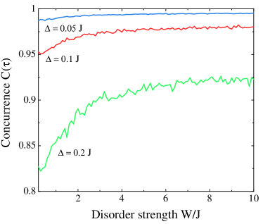
Figure 1: Two-qubit concurrence for the last cell of the ladder system, $C(\tau)$, evaluated at time $\tau=\pi N/(4J)$ against (global) disorder strength $W/J$ (from $0.2$ to $10$) averaged over $100$ distinct realizations of it. The coupling scheme was that of perfect quantum state transfer protocols Christandl et al. (2004), $J_{n}=\sqrt{n(N-n)}$. Plots were obtained by exact numerical diagonalization of Hamiltonian (II) for $N=30$ and $\Delta/J=0.05$, $0.1$, and $0.2$. The initial state was $|\psi(0)\rangle=|\mathbf{1},-\rangle$.

Figure 1 shows the disorder-averaged entanglement concurrence $C(t)$ versus disorder strength $W$ evaluated at $t=\tau$ for the encoded initial state $|\psi(0)\rangle=|\mathbf{1},-\rangle$. There we readily spot a very interesting behavior, namely that the entanglement transfer performance actually gets better upon increasing $W$. At this point it is convenient to recall that if $\Delta=0$ then the dynamics takes place on a disorder-free subspace, namely an effective ordered 1D chain (see beginning of Sec. III). In that case, the concurrence would be maximum, $C(\tau)=1$, entailing a perfect state transfer. In Fig. 1 we see that a local detuning in each cell, $\Delta\neq 0$, lowers the transfer performance. This happens because an effective internal disorder has been induced in branch $\{|\textbf{n},-\rangle\}$ at the same time information is leaking from it into $\{|\textbf{n},+\rangle\}$. We also mention that these fluctuations affect the transfer time $\tau$. On the other hand, upon increasing $W$, the concurrence is substantially recovered until saturating. At this regime, the global disorder $W$ no longer has influence on $C(\tau)$, rather, its saturated (averaged) value is set upon $\Delta$. The reason behind it is that the leakage is ultimately suppressed given $W$ is high enough as we are to discuss next.

IV.2 Leakage dynamics

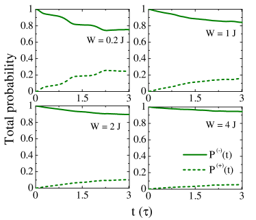
Figure 2: Time evolution of the total occupation probability in the negative branch, $P^{(-)}(t)\equiv\sum_{n}|\langle\textbf{n},-|\psi(t)\rangle|^{2}$ (solid lines), and in the positive one, $P^{(+)}(t)=1-P^{(-)}(t)$ (dashed lines), for various disorder strengths $W$, averaged over $100$ realizations of disorder. Time is expressed in units of $\tau=\pi N/(4J)$. Plots were obtained by exact numerical diagonalization of Hamiltonian (II) for $N=30$, $\Delta/J=0.2$, and $J_{n}=\sqrt{n(N-n)}$. The initial state was $|\psi(0)\rangle=|\mathbf{1},-\rangle$.

At this point, we are led to investigate the leakage of information from the anti-symmetric branch and the influence of disorder strength $W$ in order to explain the transfer (concurrence) outcomes seen in Fig. 1.

Before doing so, we shall get some intuition over the dynamics of disordered ladders by looking at its physical (original) form [Eqs. (1) and (2)]. For a moment, suppose the local energy detuning $\delta_{n}=\delta$ and $\gamma_{n}=\gamma$ for all $n$. If we set an initial state as any linear combination of, say, $\{|\mathbf{n}^{(1)}\rangle\}$, the overall occupation probability to remain in the first leg reads $P^{(1)}(t)\equiv\cos^{2}(\gamma t)$ for $\delta=0$ (see Appendix for details). Thereby, the excitation keeps oscillating back and forth between both legs periodically whereas it goes by following its own intrachain dynamics. For $\delta\neq 0$, $P^{(1)}(t)$ still undergoes periodic oscillations but with smaller amplitude and faster rate (see Eq. (15) of Appendix). The simple picture above tells us in advance that large detunings prevent leakage of information from one leg to the other, as we would have expected intuitively.

Let us now get back to the effective ladder chain described by Hamiltonian (II), wherein the local cell detunings and interchain couplings follow disordered sequences along the array. In Figure 2 we show the time evolution of $P^{(-)}(t)\equiv\sum_{n}|\langle\textbf{n},-|\psi(t)\rangle|^{2}$ for the same ladder configuration as in Fig. 1 and initial state $|\psi(0)\rangle=|\mathbf{1},-\rangle$, averaged over many distinct realizations of disorder. First and foremost, there it is clear that the disorder strength $W$ indeed prevents the excitation to leak from subspace $\{|\textbf{n},-\rangle\}$ into $\{|\textbf{n},+\rangle\}$. We shall also mention that the curves look smooth due to the disorder-averaging procedure. Each realization now displays a non-periodic oscillatory behavior. For longer times, the (averaged) total probability reaches about a stationary value which depends on both $\Delta$ and $W$.

When $\Delta\sim W$ and the system is initialized in the effective leg featuring a very low amount of disorder (that is the negative branch), the excitation spreads out far away from the initial site and so it is very likely that it will eventually find some local resonance – a given cell with low detuning $\widetilde{\epsilon}_{n,+}\approx\widetilde{\epsilon}_{n,-}$ – and therefore the excitation is capable of making through the other leg. Chances are extremely low for this to happen upon increasing $W$ and thus the excitation becomes trapped in the original leg for high enough $W\gg\Delta$.

V Conclusions

We studied a entanglement transfer protocol set over a disordered two-leg ladder qubit chain. By generating a disorder-free subspace, we carried out the protocol in the presence of local imperfections that lead to the leakage of information into the strongly-disordered manifold. We showed that increasing the disorder strength $W$ prevents such leakage thereby improving the concurrence (transfer) outcomes at the target location to a great extent. We further explained it by studying the leakage dynamics in detail.

This rather surprising behavior shows us that disorder may be an essential ingredient to prevent dissipation. Indeed, there has been considerable interest in studying open system dynamics involving structured (such as disordered) environments Lorenzo et al. (2017); Cosco et al. (2018). In Lorenzo et al. (2017), for instance – by looking at the dynamics of a single emitter coupled to an array of cavities acting as the environment – they reported that disorder pushes information back to the emitter. They further characterized this information backflow using proper non-Markovianity measures. Further extensions of our work may be taken along this direction.

Another possibility is to setting up quantum communication protocols in $N$-leg ladders for which there also exists some methods to induce a disorder-free subspace embedded within a strongly-disordered scenario Rodriguez et al. (2012).

Appendix A One-leg occupation probability

Here we show how to obtain the overall occupation probability over time in one of the legs of the physical ladder chain [Eq. (15)] given $\delta_{n}=\delta$ and $\gamma_{n}=\gamma$ for all $n$ [cf. Eqs. (1) and (2)].

Let us denote

$$|\lambda_{k,j}\rangle=\sum_{n}v_{k,n}^{(j)}|\mathbf{n}\rangle^{(j)},$$ (9)

such that it satisfies the eigenvalue equation $H^{(j)}|\lambda_{k,j}\rangle=\lambda_{k,j}|\lambda_{k,j}\rangle$, with $k=1,\ldots,N$. Now, given $J_{n,1}=J_{n,2}$, both sets of eigenstates ($j=1,2$) feature the same spatial profile. Also note that $\lambda_{k,2}=\lambda_{k,1}+\delta$. Applying the interaction Hamiltonian [Eq. (2)] thus yields $H_{I}|\lambda_{k,1(2)}\rangle=\gamma|\lambda_{k,2(1)}\rangle$. Thereby we end up with a series of independent dimer-like interactions between the normal modes of each leg and the total Hamiltonian of the system may be rewritten as $H=\sum_{k}H_{k}$, with

$$H_{k} =\lambda_{k,1}|\lambda_{k,1}\rangle\langle\lambda_{k,1}|+\lambda_{k,2}|\lambda_{k,2}\rangle\langle\lambda_{k,2}|$$

$$\,\,\,\,\,\,+\gamma(|\lambda_{k,1}\rangle\langle\lambda_{k,2}|+\mathrm{H.c.}).$$ (10)

Each dimer can be diagonalized separately and we get

$$|\psi_{k}^{\pm}\rangle=A^{\pm}|\lambda_{k,1}\rangle+B^{\pm}|\lambda_{k,2}\rangle,$$ (11)

with

$$A^{\pm}=\frac{2\gamma}{\sqrt{(\delta\pm\Omega)^{2}+4\gamma^{2}}},\,\,\,\,B^{\pm}=\frac{\delta\pm\Omega}{\sqrt{(\delta\pm\Omega)^{2}+4\gamma^{2}}},$$ (12)

and corresponding eigenenergies

$$E_{k}^{\pm}=\frac{1}{2}(\lambda_{k,1}+\lambda_{k,2}\pm\Omega)=\lambda_{k,1}+\frac{1}{2}(\delta\pm\Omega),$$ (13)

where $\Omega=\sqrt{\delta^{2}+4\gamma^{2}}$ is the effective Rabi frequency.

Now, if we initialize the system in a linear combination of the form $|\psi(0)\rangle=\sum_{k}a_{k}(0)|\lambda_{k,1}\rangle$, the time-evolved state reads

$$|\psi(t)\rangle =U(t)|\psi(0)\rangle=\sum_{k,\nu=\pm}e^{-iE_{k}^{\nu}t}|\psi_{k}^{\nu}\rangle\langle\psi_{k}^{\nu}|\psi(0)\rangle$$

$$=\sum_{\nu=\pm}(A^{\nu})^{2}e^{-i\left(\frac{\delta+\nu\Omega}{2}\right)t}\sum_{k}a_{k}(t)|\lambda_{k,1}\rangle$$

$$\,\,\,\,\,\,+\sum_{\nu=\pm}A^{\nu}B^{\nu}e^{-i\left(\frac{\delta+\nu\Omega}{2}\right)t}\sum_{k}a_{k}(t)|\lambda_{k,2}\rangle,$$ (14)

where $a_{k}(t)=a_{k}(0)e^{-i\lambda_{k}^{(1)}t}$. Therefore, the wavefunction evolves in time following the intrachain eigenspectrum – which, recall, is the same for both legs – with coefficients $a_{k}(t)$ modulated by the sums in $\nu$ (see equation above). The overall occupation probability $P^{(1)}(t)\equiv\sum_{k}|\langle\lambda_{k,1}|\psi(t)\rangle|^{2}$ can then be worked out as

$$P^{(1)}(t)=1-2\left(\frac{\gamma}{\Omega}\right)^{2}\left[1-\cos(\Omega t)\right],$$ (15)

which reduces to $P^{(1)}(t)=\cos^{2}(\gamma t)$ when $\delta=0$. Likewise, $P^{(2)}=1-P^{(1)}$ for the other leg.

References

- Apollaro et al. (2013) T. J. G. Apollaro, S. Lorenzo, and F. Plastina, Int. J. Mod. Phys. B 27, 1345035 (2013).
- Nikolopoulos and Jex (2014) G. M. Nikolopoulos and I. Jex, eds., Quantum State Transfer and Network Engineering (Springer-Verlag, Berlin, 2014).
- Bose (2003) S. Bose, Phys. Rev. Lett. 91, 207901 (2003).
- Christandl et al. (2004) M. Christandl, N. Datta, A. Ekert, and A. J. Landahl, Phys. Rev. Lett. 92, 187902 (2004).
- Plenio et al. (2004) M. B. Plenio, J. Hartley, and J. Eisert, New Journal of Physics 6, 36 (2004).
- Nikolopoulos et al. (2004) G. M. Nikolopoulos, D. Petrosyan, and P. Lambropoulos, Europhys. Lett. 65, 297 (2004).
- Burgarth and Bose (2005) D. Burgarth and S. Bose, New Journal of Physics 7, 135 (2005).
- Lorenzo et al. (2013) S. Lorenzo, T. J. G. Apollaro, A. Sindona, and F. Plastina, Phys. Rev. A 87, 042313 (2013).
- Lorenzo et al. (2015) S. Lorenzo, T. J. G. Apollaro, S. Paganelli, G. M. Palma, and F. Plastina, Phys. Rev. A 91, 042321 (2015).
- Wójcik et al. (2005) A. Wójcik, T. Łuczak, P. Kurzyński, A. Grudka, T. Gdala, and M. Bednarska, Phys. Rev. A 72, 034303 (2005).
- Wójcik et al. (2007) A. Wójcik, T. Łuczak, P. Kurzyński, A. Grudka, T. Gdala, and M. Bednarska, Phys. Rev. A 75, 022330 (2007).
- Li et al. (2005) Y. Li, T. Shi, B. Chen, Z. Song, and C.-P. Sun, Phys. Rev. A 71, 022301 (2005).
- Almeida et al. (2016) G. M. A. Almeida, F. Ciccarello, T. J. G. Apollaro, and A. M. C. Souza, Phys. Rev. A 93, 032310 (2016).
- Almeida (2018) G. M. A. Almeida, Phys. Rev. A 98, 012334 (2018).
- Allcock and Linden (2009) J. Allcock and N. Linden, Phys. Rev. Lett. 102, 110501 (2009).
- De Chiara et al. (2005) G. De Chiara, D. Rossini, S. Montangero, and R. Fazio, Phys. Rev. A 72, 012323 (2005).
- Fitzsimons and Twamley (2005) J. Fitzsimons and J. Twamley, Phys. Rev. A 72, 050301 (2005).
- Tsomokos et al. (2007) D. I. Tsomokos, M. J. Hartmann, S. F. Huelga, and M. B. Plenio, New Journal of Physics 9, 79 (2007).
- Petrosyan et al. (2010) D. Petrosyan, G. M. Nikolopoulos, and P. Lambropoulos, Phys. Rev. A 81, 042307 (2010).
- Yao et al. (2011) N. Y. Yao, L. Jiang, A. V. Gorshkov, Z.-X. Gong, A. Zhai, L.-M. Duan, and M. D. Lukin, Phys. Rev. Lett. 106, 040505 (2011).
- Zwick et al. (2011) A. Zwick, G. A. Álvarez, J. Stolze, and O. Osenda, Phys. Rev. A 84, 022311 (2011).
- Zwick et al. (2012) A. Zwick, G. A. Álvarez, J. Stolze, and O. Osenda, Phys. Rev. A 85, 012318 (2012).
- Bruderer et al. (2012) M. Bruderer, K. Franke, S. Ragg, W. Belzig, and D. Obreschkow, Phys. Rev. A 85, 022312 (2012).
- Kay (2016) A. Kay, Phys. Rev. A 93, 042320 (2016).
- Almeida et al. (2017) G. M. A. Almeida, F. A. B. F. de Moura, T. J. G. Apollaro, and M. L. Lyra, Phys. Rev. A 96, 032315 (2017).
- Almeida et al. (2018a) G. M. A. Almeida, F. A. B. F. de Moura, and M. L. Lyra, Phys. Lett. A 382, 1335 (2018a).
- Almeida et al. (2018b) G. M. A. Almeida, C. V. C. Mendes, M. L. Lyra, and F. A. B. F. de Moura, To appear in Ann. Phys. (2018b).
- Anderson (1958) P. W. Anderson, Phys. Rev. 109, 1492 (1958).
- Abrahams et al. (1979) E. Abrahams, P. W. Anderson, D. C. Licciardello, and T. V. Ramakrishnan, Phys. Rev. Lett. 42, 673 (1979).
- Dunlap et al. (1990) D. H. Dunlap, H.-L. Wu, and P. W. Phillips, Phys. Rev. Lett. 65, 88 (1990).
- Phillips and Wu (1991) P. Phillips and H.-L. Wu, Science 252, 1805 (1991).
- de Moura and Lyra (1998) F. A. B. F. de Moura and M. L. Lyra, Phys. Rev. Lett. 81, 3735 (1998).
- Izrailev and Krokhin (1999) F. M. Izrailev and A. A. Krokhin, Phys. Rev. Lett. 82, 4062 (1999).
- Kuhl et al. (2000) U. Kuhl, F. M. Izrailev, A. A. Krokhin, and H.-J. Stöckmann, Applied Physics Letters 77, 633 (2000).
- Izrailev et al. (2012) F. Izrailev, A. Krokhin, and N. Makarov, Physics Reports 512, 125 (2012).
- Sil et al. (2008a) S. Sil, S. K. Maiti, and A. Chakrabarti, Phys. Rev. Lett. 101, 076803 (2008a).
- Sil et al. (2008b) S. Sil, S. K. Maiti, and A. Chakrabarti, Phys. Rev. B 78, 113103 (2008b).
- de Moura et al. (2010) F. A. B. F. de Moura, R. A. Caetano, and M. L. Lyra, Phys. Rev. B 81, 125104 (2010).
- Rodriguez et al. (2012) A. Rodriguez, A. Chakrabarti, and R. A. Römer, Phys. Rev. B 86, 085119 (2012).
- Zhang et al. (2010) W. Zhang, R. Yang, Y. Zhao, S. Duan, P. Zhang, and S. E. Ulloa, Phys. Rev. B 81, 214202 (2010).
- Guo and Xiong (2011) A.-M. Guo and S.-J. Xiong, Phys. Rev. B 83, 245108 (2011).
- Wootters (1998) W. K. Wootters, Phys. Rev. Lett. 80, 2245 (1998).
- Bellec et al. (2012) M. Bellec, G. M. Nikolopoulos, and S. Tzortzakis, Opt. Lett. 37, 4504 (2012).
- Chapman et al. (2016) R. J. Chapman, M. Santandrea, Z. Huang, G. Corrielli, A. Crespi, M.-H. Yung, R. Osellame, and A. Peruzzo, Nat. Comm. 7, 11339 (2016).
- Lorenzo et al. (2017) S. Lorenzo, F. Lombardo, F. Ciccarello, and G. M. Palma, Scientific Reports 7, 42729 (2017).
- Cosco et al. (2018) F. Cosco, M. Borrelli, J. J. Mendoza-Arenas, F. Plastina, D. Jaksch, and S. Maniscalco, Phys. Rev. A 97, 040101 (2018).