Accelerated Coordinate Descent with Arbitrary Sampling
and Best Rates for Minibatches

Abstract

Accelerated coordinate descent is a widely popular optimization algorithm due to its efficiency on large-dimensional problems. It achieves state-of-the-art complexity on an important class of empirical risk minimization problems. In this paper we design and analyze an accelerated coordinate descent (ACD) method which in each iteration updates a random subset of coordinates according to an arbitrary but fixed probability law, which is a parameter of the method. If all coordinates are updated in each iteration, our method reduces to the classical accelerated gradient descent method AGD of Nesterov. If a single coordinate is updated in each iteration, and we pick probabilities proportional to the square roots of the coordinate-wise Lipschitz constants, our method reduces to the currently fastest coordinate descent method NUACDM of Allen-Zhu, Qu, Richtárik and Yuan.

While mini-batch variants of ACD are more popular and relevant in practice, there is no importance sampling for ACD that outperforms the standard uniform mini-batch sampling. Through insights enabled by our general analysis, we design new importance sampling for mini-batch ACD which significantly outperforms previous state-of-the-art minibatch ACD in practice. We prove a rate that is at most ${\cal O}(\sqrt{\tau})$ times worse than the rate of minibatch ACD with uniform sampling, but can be ${\cal O}(n/\tau)$ times better, where $\tau$ is the minibatch size. Since in modern supervised learning training systems it is standard practice to choose $\tau\ll n$, and often $\tau={\cal O}(1)$, our method can lead to dramatic speedups. Lastly, we obtain similar results for minibatch nonaccelerated CD as well, achieving improvements on previous best rates.

1 Introduction

Many key problems in machine learning and data science are routinely modeled as optimization problems and solved via optimization algorithms. With the increase of the volume of data used to formulate optimization models, there is a need for new efficient algorithms able to cope with the challenge. Through intensive research and algorithmic innovation during the last 10-15 years, gradient methods have become the methods of choice for large-scale optimization problems.

In this paper we consider the optimization problem

$$\min_{x\in\mathbb{R}^{n}}f(x),$$ (1)

where $f$ a smooth and strongly convex function, and the main difficulty comes from the dimension $n$ being very large (e.g., millions or billions). In this regime, coordinate descent (CD) variants of gradient methods are the state of the art.

The simplest variant of CD in each iterations updates a single variable of $x$ by taking a one dimensional gradient step along the direction of $i$th unit basis vector $e_{i}\in\mathbb{R}^{n}$, which leads to the update rule

$$\boxed{x^{k+1}=x^{k}-\alpha_{i}\nabla_{i}f(x^{k})e_{i}}$$ (2)

where $\nabla_{i}f(x^{k}):=e_{i}^{\top}\nabla f(x^{k})$ is the $i$th partial derivative and $\alpha_{i}$ is a suitably chosen stepsize. The classical smoothness assumption used in the analysis of CD methods [16] is to require the existence of constants $L_{i}>0$ such that

$$f(x+te_{i})\leq f(x)+t\nabla_{i}f(x)+\frac{L_{i}}{2}t^{2}$$ (3)

holds for all $x\in\mathbb{R}^{n}$, $t\in\mathbb{R}$ and $i\in[n]:=\{1,2,\dots,n\}$. In this setting, one can choose the stepsizes to be $\alpha_{i}=1/L_{i}$.

There are several rules studied in the literature for choosing the coordinate $i$ in iteration $k$, including cyclic rule [12, 31, 25, 32, 9], Gauss-Southwell or other greedy rules [17, 33, 29], random (stationary) rule [16, 23, 24, 28, 11, 8] and adaptive random rules [5, 30]. In this work we focus on stationary random rules, which are popular by practitioners and well understood in theory.

Updating one coordinate at a time. The simplest randomized CD method of the form (2) chooses coordinate $i$ in each iteration uniformly at random. If $f$ is $\sigma$–convex, then this method converges in $(n\max_{i}L_{i}/\sigma)\log(1/\epsilon)$ iterations in expectation. If index $i$ is chosen with probability $p_{i}\propto L_{i}$, then the iteration complexity improves to $(\sum_{i}L_{i}/\sigma)\log(1/\epsilon)$. The latter result is always better than the former, and can be up to $n$ times better. These results were established in a seminal paper by Nesterov [16]. The analysis was later generalized to arbitrary probabilities $p_{i}>0$ by Richtárik and Takáč [23], who obtained the complexity

$$\left(\max_{i}\frac{L_{i}}{p_{i}\sigma}\right)\log\frac{1}{\epsilon}.$$ (4)

Clearly, (4) includes the previous two results as special cases. Note that the importance sampling $p_{i}\propto L_{i}$ minimizes the complexity bound (4) and is therefore in this sense optimal.

Mini-batching: updating more coordinates at a time. In many situations it is advantageous to update a small subset (mini-batch) of coordinates in each iteration, which leads to the mini-batch CD method which has the form

$$\boxed{x^{k+1}_{i}=\begin{cases}x^{k}_{i}-\alpha_{i}\nabla_{i}f(x^{k})&\quad i\in S^{k},\\ x^{k}_{i}&\quad i\notin S^{k}.\end{cases}}$$ (5)

For instance, it is often equally easy to fetch information about a small batch of coordinates $S^{k}$ from memory at the same or comparable time as it is to fetch information about a single coordinate. If this memory access time is the bottleneck as opposed to computing the actual updates to coordinates $i\in S^{k}$, then it is more efficient to update all coordinates belonging to the mini-batch $S^{k}$. Alternatively, in situations where parallel processing is available, one is able to compute the updates to a small batch of coordinates simultaneously, leading to speedups in wall clock time. With this application in mind, mini-batch CD methods are also often called parallel CD methods [24].

2 Arbitrary sampling and mini-batching

Arbitrary sampling. Richtárik and Takáč [24] analyzed method (5) for uniform samplings $S^{k}$, i.e., assuming that $\mathbb{P}(i\in S^{k})=\mathbb{P}(j\in S^{k})$ for all $i,j$. However, the ultimate generalization is captured by the notion of arbitrary sampling pioneered by Richtárik and Takáč [22]. A sampling refers to a set-valued random mapping $S$ with values being the subsets of $[n]$. The word arbitrary refers to the fact that no additional assumptions on the sampling, such as uniformity, are made. This result generalizes the results mentioned above.

For mini-batch CD methods it is useful to assume a more general notion of smoothness parameterized by a positive semidefinite matrix ${\bf M}\in\mathbb{R}^{n\times n}$. We say that $f$ is ${\bf M}$–smooth if

$$f(x+h)\leq f(x)+\nabla f(x)^{\top}h+\frac{1}{2}h^{\top}{\bf M}h$$ (6)

for all $x,h\in\mathbb{R}^{n}$. Given a sampling $S$ and ${\bf M}$–smooth function $f$, let $v=(v_{1},\dots,v_{n})$ be positive constants satisfying the ESO (expected separable overapproximation) inequality

$${\bf P}\circ{\bf M}\preceq\mathbf{Diag}\left(p_{1}v_{1},\dots,p_{n}v_{n}\right),$$ (7)

where ${\bf P}$ is the probability matrix associated with sampling $S$, defined by ${\bf P}_{ij}:=\mathbb{P}(i\in S\;\&\;j\in S)$, $p_{i}:={\bf P}_{ii}=\mathbb{P}(i\in S)$ and $\circ$ denotes the Hadamard (i.e., elementwise) product of matrices. From now on we define the probability vector as $p:=(p_{1},\dots,p_{n})\in\mathbb{R}^{n}$ and let $v=(v_{1},\dots,v_{n})\in\mathbb{R}^{n}$ be the vector of ESO parameters. With this notation, (7) can be equivalently written as ${\bf P}\circ{\bf M}\preceq\mathbf{Diag}\left(p\circ v\right)$. We say that $S$ is proper if $p_{i}>0$ for all $i$.

It can be show by combining the results from [22] and [19] that under the above assumptions, the minibatch CD method (5) with stepsizes $\alpha_{i}=1/v_{i}$ enjoys the iteration complexity

$$\left(\max_{i}\frac{v_{i}}{p_{i}\sigma}\right)\log\frac{1}{\epsilon}.$$ (8)

Since in situations when $|S^{k}|=1$ with probability 1 once can choose $v_{i}=L_{i}$, the complexity result (8) generalizes (4). Inequality (7) is standard in minibatch coordinate descent literature. It was studied extensively in [19], and has been used to analyze parallel CD methods [24, 22, 8], distributed CD methods [21, 7], accelerated CD methods in [8, 7, 18, 3], and dual methods [20, 3].

Importance sampling for mini-batches. It is easy to see, for instance, that if we do not restrict the class of samplings over which we optimize, then the trivial full sampling $S^{k}=[n]$ with probability 1 is optimal. For this sampling, ${\bf P}$ is the matrix of all ones, $p_{i}=1$ for all $i$, and (7) holds for $v_{i}=L:=\lambda_{\max}({\bf M})$ for all $i$. The mini-batch CD method (5) reduces to gradient descent, and the complexity estimate (8) becomes $(L/\sigma)\log(1/\epsilon)$, which is the standard rate of gradient descent. However, typically we are interested in finding the best sampling from the class of samplings which use a mini-batch of size $\tau$, where $\tau\ll n$. While we have seen that the importance sampling $p_{i}=L_{i}/\sum_{j}L_{j}$ is optimal for $\tau=1$, in the mini-batch case $\tau>1$ the problem of determining a sampling which minimizes the bound (8) is much more difficult. For instance, [22] consider a certain parametric family of samplings where the problem of finding the best sampling from this family reduces to a linear program.

Surprisingly, and in contrast to the situation in the $\tau=1$ case where an optimal sampling is known and is in general non-uniform, there is no mini-batch sampling that is guaranteed to outperform $\tau$–nice sampling. We say that $S$ is $\tau$–nice if it samples uniformly from among all subsets of $[n]$ of cardinality $\tau$. The probability matrix of this sampling is given by

$${\bf P}=\frac{\tau}{n}\left((1-\beta){\bf I}+\beta{\bf E}\right),$$

where $\beta=\tfrac{\tau-1}{n-1}$ (assume $n>1$) and ${\bf E}$ is the matrix of all ones, and $p_{i}=\tfrac{\tau}{n}$ [19]. It follows that the ESO inequality (7) holds for $v_{i}=(1-\beta){\bf M}_{ii}+\beta L.$ By plugging into (8), we get the iteration complexity

$$\frac{n}{\tau}\left(\frac{(1-\beta)\max_{i}{\bf M}_{ii}+\beta L}{\sigma}\right)\log\frac{1}{\epsilon}.$$ (9)

This rate interpolates between the rate of CD with uniform probabilities (for $\tau=1$) and the rate of gradient descent (for $\tau=n$).

	CD	ACD
$\tau=1$, $p_{i}>0$	$\left(\max_{i}\frac{L_{i}}{p_{i}\sigma}\right)\log\frac{1}{\epsilon}$ [23]	$\sqrt{\max_{i}\frac{L_{i}}{p_{i}^{2}\sigma}}\log\frac{1}{\epsilon}$ [this paper]
$\tau=1$, best $p_{i}$	$\frac{\sum_{i}L_{i}}{\sigma}\log\frac{1}{\epsilon}$;  $p_{i}\propto L_{i}$ [16]	$\frac{\sum_{i}\sqrt{L_{i}}}{\sqrt{\sigma}}\log\frac{1}{\epsilon}$;  $p_{i}\propto\sqrt{L_{i}}$ [2]
arbitrary sampling	$\left(\max_{i}\frac{v_{i}}{p_{i}\sigma}\right)\log\frac{1}{\epsilon}$ [22]	$\sqrt{\max_{i}\frac{v_{i}}{p_{i}^{2}\sigma}}\log\frac{1}{\epsilon}$ [this paper]

Table 1: Complexity results for CD and ACD methods for $\sigma$–convex functions.

3 Contributions

For accelerated coordinate descent (ACD) without mini-batching (i.e., when $\tau=1$), the currently best known iteration complexity result, due to Allen-Zhu et al [2], is

$${\cal O}\left(\frac{\sum_{i}\sqrt{L_{i}}}{\sqrt{\sigma}}\log\frac{1}{\epsilon}\right).$$ (10)

The probabilities used in the algorithm are proportional to the square roots of the coordinate-wise Lipschitz constants: $p_{i}\propto\sqrt{L_{i}}$. This is the first CD method with a complexity guarantee which does not explicitly depend on the dimension $n$, and is an improvement on the now-classical result of Nesterov [16] giving the complexity

$${\cal O}\left(\sqrt{\frac{n\sum_{i}L_{i}}{\sigma}}\log\frac{1}{\epsilon}\right).$$

The rate (10) is always better than this, and can be up to $\sqrt{n}$ times better if the distribution of $L_{i}$ is extremely non-uniform. Unlike in the non-accelerated case described in the previous section, there is no complexity result for ACD with general probabilities such as (4), or with an arbitrary sampling such as (8). In fact, an ACD method was not even designed in such settings, despite a significant recent development in accelerated coordinate descent methods [13, 10, 11, 18, 2].

Our key contributions are:

$\diamond$ ACD with arbitrary sampling. We design an ACD method which is able to operate with an arbitrary sampling of subsets of coordinates. We describe our method in Section 4.

$\diamond$ Iteration complexity. We prove (see Theorem 4.2) that the iteration complexity of ACD is

$${\cal O}\left(\sqrt{\max_{i}\frac{v_{i}}{p_{i}^{2}\sigma}}\log\frac{1}{\epsilon}\right),$$ (11)

where $v_{i}$ are ESO parameters given by (7) and $p_{i}>0$ is the probability that coordinate $i$ belongs to the sampled set $S^{k}$: $p_{i}:=\mathbb{P}(i\in S^{k})$. The result of Allen-Zhu et al. (10) (NUACDM) can be recovered as a special case of (11) by focusing on samplings defined by $S^{k}=\{i\}$ with probability $p_{i}\propto\sqrt{L_{i}}$ (recall that in this case $v_{i}=L_{i}$). When $S^{k}=[n]$ with probability 1, then our method reduces to accelerated gradient descent (AGD) [14, 15], and since $p_{i}=1$ and $v_{i}=L$ (the Lipschitz constant of $\nabla f$) for all $i$, (11) reduces to the standard complexity of AGD: ${\cal O}(\sqrt{L/\sigma}\log(1/\epsilon)).$

$\diamond$ Weighted strong convexity. In fact, we prove a more general result than (11) in which we allow the strong convexity of $f$ to be measured in a weighted Euclidean norm with weights $v_{i}/p_{i}^{2}$. In situations when $f$ is naturally strongly convex with respect to a weighted norm, this more general result will typically lead to a better complexity result than (11), which is fine-tuned for standard strong convexity. There are applications when $f$ is naturally a strongly convex with respect to some weighted norm [2].

$\diamond$ Mini-batch methods. We design several new importance samplings for mini-batches, calculate the associated complexity results, and show through experiments that they significantly outperform the standard uniform samplings used in practice and constitute the state of the art. Our importance sampling leads to rates which are provably within a small factor from the best known rates, but can lead to an improvement by a factor of ${\cal O}(n)$. We are the first to establish such a result, both for CD (Appendix B) and ACD (Section 5).

The key complexity results obtained in this paper are summarized and compared to prior results in Table 1.

4 The algorithm

The accelerated coordinate descent method (ACD) we propose is formalized as Algorithm 1. As mentioned before, we will analyze our method under a more general strong convexity assumption.

Assumption 4.1.

$f$ is $\sigma_{w}$–convex with respect to the $\|\cdot\|_{w}$ norm. That is,

$$f(x+h)\geq f(x)+\langle\nabla f(x),h\rangle+\frac{\sigma_{w}}{2}\|h\|_{w}^{2},$$ (12)

for all $x,h\in\mathbb{R}^{n}$, where $\sigma_{w}>0$.

Note that if $f$ is $\sigma$–convex in the standard sense (i.e., for $w=(1,\dots,1)$), then $f$ is $\sigma_{w}$–convex for any $w>0$ with $\sigma_{w}=\min_{i}\frac{\sigma}{w_{i}}.$

Input: i.i.d. proper samplings $S^{k}\sim{\cal D}$; $v,w\in\mathbb{R}^{n}_{++}$; $\sigma_{w}>0$; stepsize parameters $\eta,\theta>0$

Initialize: Initial iterate $y^{0}=z^{0}\in\mathbb{R}^{n}$

for $k=0,1\dots$ do

      

$$x^{k+1}=(1-\theta)y^{k}+\theta z^{k}$$ (13)

$$\text{Get }S^{k}\sim{\cal D}$$ (14)

$$y^{k+1}=x^{k+1}-\sum_{i\in S^{k}}\frac{1}{v_{i}}\nabla_{i}f(x^{k+1})e_{i}$$ (15)

$$z^{k+1}=\frac{1}{1+\eta\sigma_{w}}\left(z^{k}+\eta\sigma_{w}x^{k+1}-\sum_{i\in S^{k}}\frac{\eta}{p_{i}w_{i}}\nabla_{i}f(x^{k+1})e_{i}\right)$$ (16)

end for

Algorithm 1 ACD (Accelerated coordinate descent with arbitrary sampling)

Using the tricks developed in [10, 8, 11], Algorithm 1 can be implemented so that only $|S^{k}|$ coordinates are updated in each iteration. We are now ready derive a convergence rate of ACD.

Theorem 4.2 (Convergence of ACD).

Let $S^{k}$ be i.i.d. proper (but otherwise arbitrary) samplings. Let ${\bf P}$ be the associated probability matrix and $p_{i}:=\mathbb{P}(i\in S^{k})$. Assume $f$ is ${\bf M}$–smooth (see (6)) and let $v$ be ESO parameters satisfying (7). Further, assume that $f$ is $\sigma_{w}$–convex (with $\sigma_{w}>0$) for

$$w_{i}:=\frac{v_{i}}{p_{i}^{2}},\qquad i=1,2,\dots,n,$$ (17)

with respect to the weighted Euclidean norm $\|\cdot\|_{w}$ (i.e., we enforce Assumption 4.1). Then

$$\sigma_{w}\leq\frac{{\bf M}_{ii}p_{i}^{2}}{v_{i}}\leq p_{i}^{2}\leq 1,\qquad i=1,2,\dots n.$$ (18)

In particular, if $f$ is $\sigma$–convex with respect to the standard Euclidean norm, then we can choose

$$\sigma_{w}=\min_{i}\frac{p_{i}^{2}\sigma}{v_{i}}.$$ (19)

Finally, if we choose

$$\theta:=\frac{\sqrt{\sigma_{w}^{2}+4\sigma_{w}}-\sigma_{w}}{2}=\frac{2\sigma_{w}}{\sqrt{\sigma_{w}^{2}+4\sigma_{w}}+\sigma_{w}}\geq 0.618\sqrt{\sigma_{\omega}}$$ (20)

and $\eta:=\frac{1}{\theta},$ then the random iterates of ACD satisfy

$$\mathbb{E}\left[P^{k}\right]\leq(1-\theta)^{k}P^{0},$$ (21)

where $P^{k}:=\frac{1}{\theta^{2}}\left(f(y^{k})-f(x^{*})\right)+\frac{1}{2(1-\theta)}\|z^{k}-x^{*}\|_{w}^{2}$ and $x^{*}$ is the optimal solution of (1).

Noting that $1/0.618\leq 1.619$, as an immediate consequence of (21) and (20) we get bound

$$k\geq\frac{1.619}{\sqrt{\sigma_{w}}}\log\frac{1}{\epsilon}\quad\Rightarrow\quad\mathbb{E}\left[P^{k}\right]\leq\epsilon P^{0}.$$ (22)

If $f$ is $\sigma$–convex, then by plugging (19) into (22) we obtain the iteration complexity bound

$$1.619\cdot\sqrt{\max_{i}\frac{v_{i}}{p_{i}^{2}\sigma}}\log\frac{1}{\epsilon}.$$ (23)

Complexity (23) is our key result (also mentioned in (11) and Table 1).

5 Importance sampling for mini-batches

Let $\tau:=\mathbb{E}\left[|S^{k}|\right]$ be the expected mini-batch size. The next theorem provides an insightful lower bound for the complexity of ACD we established, one independent of $p$ and $v$.

Theorem 5.1 (Limits of mini-batch performance).

Let the assumptions of Theorem 4.2 be satisfied and let $f$ be $\sigma$–convex. Then the dominant term in the rate (23) of ACD admits the lower bound

$$\sqrt{\max_{i}\frac{v_{i}}{p_{i}^{2}\sigma}}\geq\frac{\sum_{i}\sqrt{{\bf M}_{ii}}}{\tau\sqrt{\sigma}}.$$ (24)

Note that for $\tau=1$ we have ${\bf M}_{ii}=v_{i}=L_{i}$, and the lower bound is achieved by using the importance sampling $p_{i}\propto\sqrt{L_{i}}$. Hence, this bound gives a limit on how much speedup, compared to the best known complexity in the $\tau=1$ case, we can hope for as we increase $\tau$. The bound says we can not hope for better than linear speedup in the mini-batch size. An analogous result (obtained by removing all the squares and square roots in (24)) was established in [22] for CD.

In what follows, it will be useful to write the complexity result (23) in a new form by considering a specific choice of the ESO vector $v$.

Lemma 5.2.

Choose any proper sampling $S$ and let ${\bf P}$ be its probability matrix and $p$ its probability vector. Let $c(S,{\bf M}):=\lambda_{\max}({\bf P}^{\prime}\circ{\bf M}^{\prime})$, where ${\bf P}^{\prime}:={\bf D}^{-1/2}{\bf P}{\bf D}^{-1/2}$, ${\bf M}^{\prime}:={\bf D}^{-1}{\bf M}{\bf D}^{-1}$ and ${\bf D}:=\mathbf{Diag}\left(p\right)$. Then the vector $v$ defined by $v_{i}=c(S,{\bf M})p_{i}^{2}$ satisfies the ESO inequality (7) and the total complexity (23) becomes

$$1.619\cdot\frac{\sqrt{c(S,{\bf M})}}{\sqrt{\sigma}}\log\frac{1}{\epsilon}.$$ (25)

Since $\tfrac{1}{n}{\rm Trace}\left({\bf P}^{\prime}\circ{\bf M}^{\prime}\right)\leq c(S,{\bf M})\leq{\rm Trace}\left({\bf P}^{\prime}\circ{\bf M}^{\prime}\right)$ and ${\rm Trace}\left({\bf P}^{\prime}\circ{\bf M}^{\prime}\right)=\sum_{i}{\bf P}^{\prime}_{ii}{\bf M}^{\prime}_{ii}=\sum_{i}{\bf M}^{\prime}_{ii}=\sum_{i}{\bf M}_{ii}/p_{i}^{2}$, we get the bounds:

$$\sqrt{\frac{1}{n}\sum_{i}\frac{{\bf M}_{ii}}{p_{i}^{2}\sigma}}\log\frac{1}{\epsilon}\leq\sqrt{\frac{c(S,{\bf M})}{\sigma}}\log\frac{1}{\epsilon}\leq\sqrt{\sum_{i}\frac{{\bf M}_{ii}}{p_{i}^{2}\sigma}}\log\frac{1}{\epsilon}.$$ (26)

5.1 Sampling 1: standard uniform minibatch samlpling ($\tau$–nice sampling)

Let $S_{1}$ be the $\tau$-nice sampling. It can be shown (see Lemma C.3) that $c(S_{1},{\bf M})\leq\frac{n^{2}}{\tau^{2}}((1-\beta)\max_{i}{\bf M}_{ii}+\beta L)$, and hence the iteration complexity (23) becomes

$${\cal O}\left(\frac{n}{\tau}\sqrt{\frac{(1-\beta)\max_{i}{\bf M}_{ii}+\beta L}{\sigma}}\log\frac{1}{\epsilon}\right).$$ (27)

This result interpolates between ACD with uniform probabilities (for $\tau=1$) and accelerated gradient descent (for $\tau=n$). Note that the rate (27) is a strict improvement on the CD rate (9).

5.2 Sampling 2: importance sampling for minibatches

Consider now the sampling $S_{2}$ which includes every $i\in[n]$ in $S_{2}$, independently, with probability

$$p_{i}=\tau\frac{\sqrt{{\bf M}_{ii}}}{\sum_{j}\sqrt{{\bf M}_{jj}}}.$$

This sampling was not considered in the literature before. Note that $\mathbb{E}\left[|S_{2}|\right]=\sum_{i}p_{i}=\tau$. For this sampling, bounds (26) become:

$$\frac{\sum_{i}\sqrt{{\bf M}_{ii}}}{\tau\sqrt{\sigma}}\log\frac{1}{\epsilon}\leq\sqrt{\frac{c(S,{\bf M})}{\sigma}}\log\frac{1}{\epsilon}\leq\frac{\sqrt{n}\sum_{i}\sqrt{{\bf M}_{ii}}}{\tau\sqrt{\sigma}}\log\frac{1}{\epsilon}.$$ (28)

Clearly, with this sampling we obtain an ACD method with complexity within a $\sqrt{n}$ factor from the lower bound established in Theorem 5.1. For $\tau=1$ we have ${\bf P}^{\prime}={\bf I}$ and hence $c(S,{\bf M})=\lambda_{\max}({\bf I}\circ{\bf M}^{\prime})=\lambda_{\max}(\mathbf{Diag}\left({\bf M}^{\prime}\right))=\max_{i}{\bf M}_{ii}/p_{i}^{2}=(\sum_{j}\sqrt{{\bf M}_{jj}})^{2}$. Thus, the rate of ACD achieves the lower bound in (28) (see also (10)) and we recover the best current rate of ACD in the $\tau=1$ case, established in [2]. However, the sampling has an important limitation: it can be used for $\tau\leq\sum_{j}\sqrt{{\bf M}_{jj}}/\max_{i}{\bf M}_{ii}$ only as otherwise the probabilities $p_{i}$ exceed 1.

5.3 Sampling 3: another importance sampling for minibatches

Now consider sampling $S_{3}$ which includes each coordinate $i$ within $S_{3}$ independently, with probability $p_{i}$ satisfying the relation $p_{i}^{2}/{\bf M}_{ii}\propto 1-p_{i}$. This is equivalent to setting

$$p_{i}:=\frac{2{\bf M}_{ii}}{\sqrt{{\bf M}_{ii}^{2}+2{\bf M}_{ii}\delta}+{\bf M}_{ii}},$$ (29)

where $\delta$ is a scalar for which $\sum_{i}p_{i}=\tau$. This sampling was not considered in the literature before. Probability vector $p$ was chosen as (29) for two reasons: i) $p_{i}\leq 1$ for all $i$, and therefore the sampling can be used for all $\tau$ in contrast to $S_{1}$, and ii) we can prove Theorem 5.3.

Let $c_{1}:=c(S_{1},{\bf M})$ and $c_{3}:=c(S_{3},{\bf M})$. In light of (25), Theorem 5.3 compares $S_{1}$ and $S_{3}$ and says that ACD with $S_{3}$ has at most ${\cal O}(\sqrt{\tau})$ times worse rate compared to ACD with $S_{1}$, but has the capacity to be ${\cal O}(n/\tau)$ times better. We prove in Appendix B a similar theorem for CD. We stress that, despite some advances in the development of importance samplings for minibatch methods [22, 6], $S_{1}$ was until now the state-of-the-art in theory for CD. We are the first to give a provably better rate in the sense of Theorem B.3. The numerical experiments show that $S_{3}$ consistently outperforms $S_{1}$, and often dramatically so.

Theorem 5.3.

The leading complexity terms $c_{1}$ and $c_{3}$ of ACD (Algorithm (5)) with samplings $S_{1}$, and $S_{3}$, respectively, defined in Lemma 5.2, compare as follows:

$$c_{3}\leq 2\frac{(2n-\tau)(n\tau+n-\tau)}{(n-\tau)^{2}}c_{1}={\cal O}(\tau)c_{1}.$$ (30)

Moreover, there exists ${\bf M}$ where $c_{3}\leq{\cal O}(\tfrac{\tau^{2}}{n^{2}})c_{1}$.

In real world applications, minibatch size $\tau$ is limited by hardware and in typical situations one has $\tau\ll n$, oftentimes $\tau={\cal O}(1)$. The importance of Theorem 5.3 is best understood from this perspective.

Lower bound	$S_{1}$: $p_{i}=\tfrac{\tau}{n}$	$S_{2}:\tfrac{p_{i}^{2}}{{\bf M}_{ii}}\propto 1$	$S_{3}:\tfrac{p_{i}^{2}}{{\bf M}_{ii}}\propto 1-p_{i}$
$\tfrac{\sum_{i}\sqrt{{\bf M}_{ii}}}{\tau\sqrt{\sigma}}$	$\tfrac{n\sqrt{(1-\beta)\max_{i}{\bf M}_{ii}+\beta L}}{\tau\sqrt{\sigma}}$	$\tfrac{\gamma\sum_{i}\sqrt{{\bf M}_{ii}}}{\tau\sqrt{\sigma}}$	$\omega\tfrac{n\sqrt{(1-\beta)\max_{i}{\bf M}_{ii}+\beta L}}{\tau\sqrt{\sigma}}$
(24)	= uniform ACD for $\tau=1$ = AGD for $\tau=n$	$\leq\sqrt{n}\times$ lower bound $\bullet$ $\tau\leq\tfrac{\sum_{j}\sqrt{{\bf M}_{jj}}}{\max_{i}{\bf M}_{ii}}$	$\bullet$ fastest in practice $\bullet$ any $\tau$ allowed

Table 2: New complexity results for ACD with mini-batch size $\tau=\mathbb{E}\left[|S^{k}|\right]$ and various samplings (we suppress $\log(1/\epsilon)$ factors in all expressions). Constants: $\sigma=$ strong convexity constant of $f$, $L=\lambda_{\max}({\bf M})$, $\beta=(\tau-1)/(n-1)$, $1\leq\gamma\leq\sqrt{n}$, and $\omega\leq{\cal O}(\sqrt{\tau})$ ($\omega$ can be as small as ${\cal O}(\tau/n)$).

6 Experiments

We perform extensive numerical experiments to justify that minibatch ACD with importance sampling works well in practice. Here we present a few selected experiment only; more can be found in Appendix D.

In most of plots we compare of both accelerated and non-accelerated CD with all samplings $S_{1},S_{2},S_{3}$ introduced in Sections 5.1, 5.2 and 5.3 respectively. We refer to ACD with sampling $S_{3}$ as AN (Accelerated Nonuniform), ACD with sampling $S_{1}$ as AU, ACD with sampling $S_{2}$ as AN2, CD with sampling $S_{3}$ as NN, CD with sampling $S_{1}$as NU and CD with sampling $S_{2}$ as NN2. We compare the methods for various choices of the expected minibatch sizes $\tau$ and on several problems.

In Figure 1, we report on a logistic regression problem with a few selected LibSVM [4] datasets. For larger datasets, pre-computing both strong convexity parameter $\sigma$ and $v$ may be expensive (however, recall that for $v$ we need to tune only one scalar). Therefore, we choose ESO parameters $v$ from Lemma 5.2, while estimating the smoothness matrix as $10\times$ its diagonal. An estimate of the strong convexity $\sigma$ for acceleration was chosen to be the minimal diagonal element of the smoothness matrix. We provide a formal formulation of the logistic regression problem, along with more experiments applied to further datasets in Appendix D.2, where we choose $v$ and $\sigma$ in full accord with the theory.

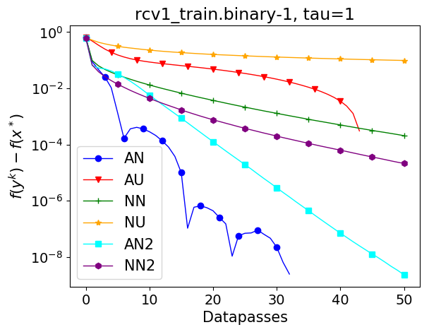
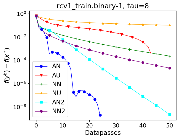
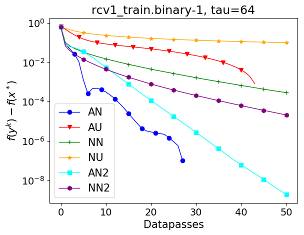
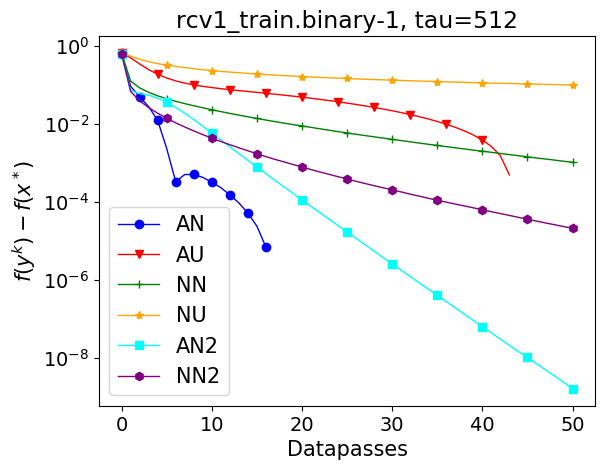
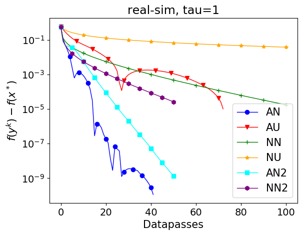
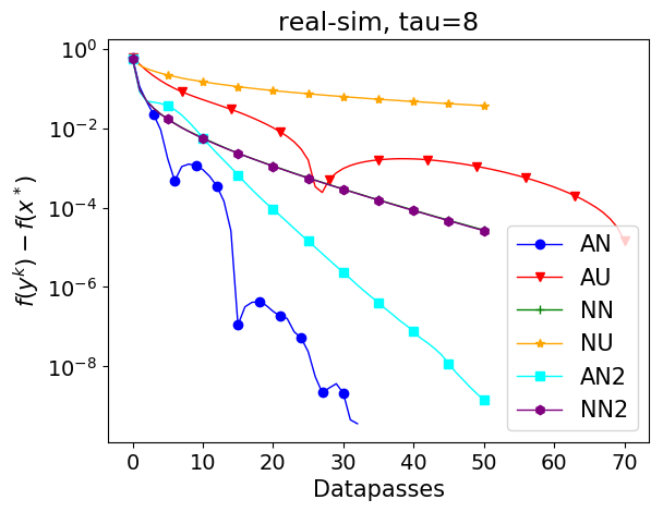
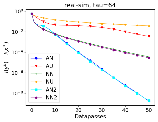
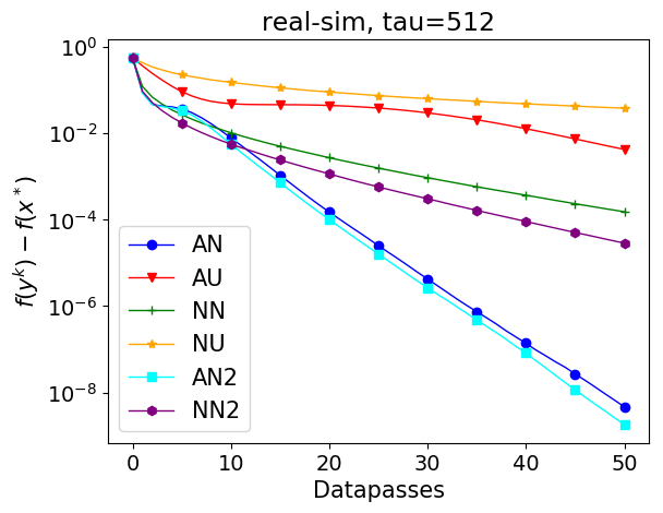
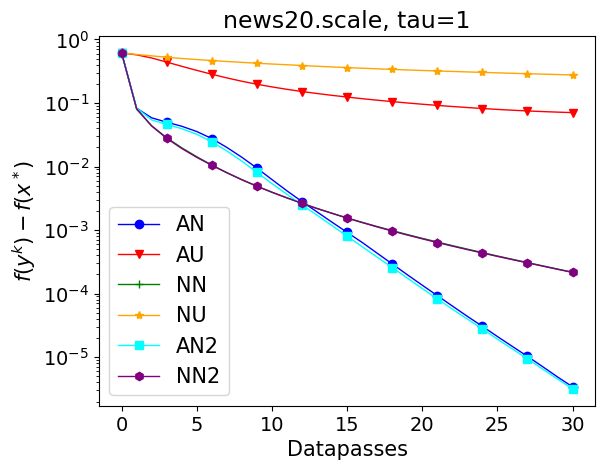
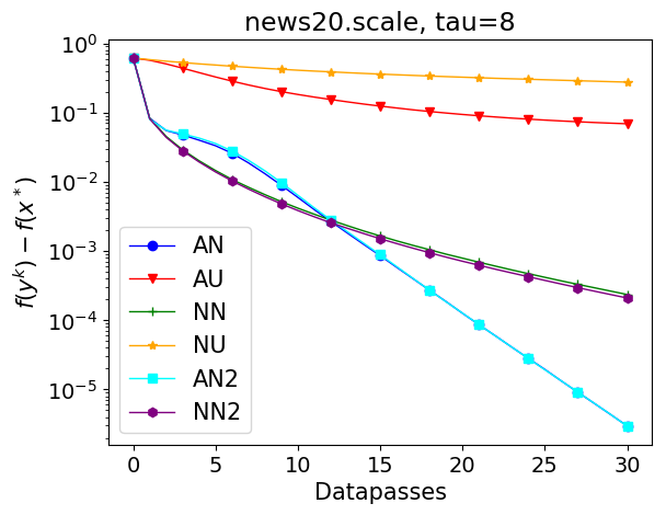
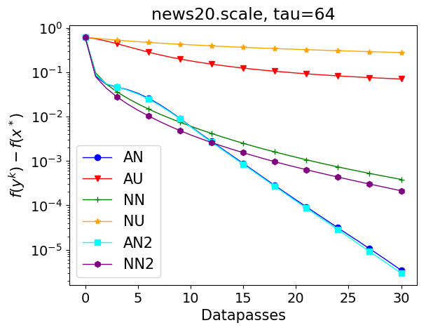
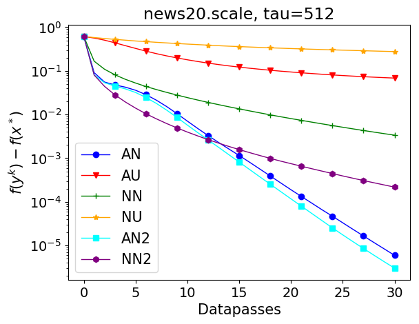
Figure 1: Six variants of coordinate descent (AN, AU, NN, NU, AN2 and AU2) applied to a logistic regression problem, with minibatch sizes $\tau=1,8,64$ and $512$.

Coordinate descent methods which allow for separable proximal operator were proven to be efficient to solve ERM problem, when applied on dual [26, 27, 28, 35]. Although we do not develop proximal methods in this paper, we empirically demonstrate that ACD allows for this extension as well. As a specific problem to solve, we choose dual of SVM with hinge loss. The results and a detailed description of the experiment are presented in Appendix D.3, and are indeed in favour of ACD with importance sampling. Therefore, ACD is not only suitable for big dimensional problems, it can handle the big data setting as well.

Finally, in Appendix D.1 we present several synthetic examples in order to shed more light on acceleration and importance sampling, and to see how its performance depends on the data. We also study how minibatch size influences the convergence rate. All the experimental results clearly show that acceleration, importance sampling and minibatching have a significant impact on practical performance of CD methods. Moreover, the difference in the performance of samplings $S_{2}$ and $S_{3}$ is negligible, and therefore we recommend using $S_{3}$, as it is not limited by the bound on expected minibatch sice $\tau$

Appendix

Appendix A Proof of Theorem 4.2

Before starting the proof, we mention that the proof technique we use is inspired by [1, 2], which takes the advantage of the coupling of gradient descent with mirror descent, resulting in a relatively simple proof.

A.1 Proof of inequality (18)

By comparing (12) and (6) for $h=e_{i}$, we get $\sigma_{w}w_{i}\leq{\bf M}_{ii}$, and the first inequality in (18) follows. Using (7) it follows that $e_{i}^{\top}({\bf P}\circ{\bf M})e_{i}\preceq e_{i}^{\top}\mathbf{Diag}\left(p\circ v\right)e_{i}$, which in turn implies ${\bf M}_{ii}\leq v_{i}$ and the second inequality in (18) follows.

A.2 Descent lemma

The following lemma is a consequence of ${\bf M}$–smoothness of $f$, and ESO inequality (7).

Lemma A.1.

Under the assumptions of Theorem 4.2, for all $k\geq 0$ we have the bound

$$f(x^{k+1})-\mathbb{E}\left[f(y^{k+1})\,|\,x^{k+1}\right]\geq\frac{1}{2}\|\nabla f(x^{k+1})\|^{2}_{v^{-1}\circ p}.$$ (31)

Proof.

We have

$$\mathbb{E}\left[f(y^{k+1})\right] \stackrel{{\scriptstyle\eqref{eq:y_update}}}{{=}} \mathbb{E}\left[f\left(x^{k+1}-\sum_{i\in S^{k}}\frac{1}{v_{i}}\nabla_{i}f(x^{k+1}\right)e_{i})\right]$$

$$\stackrel{{\scriptstyle\eqref{eq:M-smooth-intro}}}{{\leq}} f(x^{k+1})-\|\nabla f(x^{k+1})\|^{2}_{v^{-1}\circ p}+\frac{1}{2}\mathbb{E}\left[\left\|\sum_{i\in S^{k}}\frac{1}{v_{i}}\nabla_{i}f(x^{k+1})e_{i}\right\|^{2}_{{\bf M}}\right]$$

$$\stackrel{{\scriptstyle\eqref{eq:v_def}}}{{\leq}} f(x^{k+1})-\|\nabla f(x^{k+1})\|^{2}_{v^{-1}\circ p}+\frac{1}{2}\left\|\nabla f(x^{k+1})\right\|^{2}_{v^{-1}\circ p}.$$

∎

A.3 Key technical inequality

We first establish a lemma which will play a key part in the analysis.

Lemma A.2.

For every $u$ we have

$$\eta\sum_{i\in S^{k}}\left\langle\frac{1}{p_{i}}\nabla_{i}f(x^{k+1})e_{i},z^{k+1}-u\right\rangle-\frac{\eta\sigma_{w}}{2}\|x^{k+1}-u\|^{2}_{w}$$

$$\qquad\qquad\leq-\frac{1}{2}\|z^{k}-z^{k+1}\|^{2}_{w}+\frac{1}{2}\|z^{k}-u\|_{w}^{2}-\frac{1+\eta\sigma_{w}}{2}\|z^{k+1}-u\|^{2}_{w}.$$

Proof.

The proof is a direct generalization of the proof of analogous lemma in [2]. We include it for completeness. Notice that (16) is equivalent to

$$z^{k+1}=\operatorname{argmin}_{z}h^{k}(z):=\operatorname{argmin}_{z}\frac{1}{2}\|z-z^{k}\|^{2}_{w}+\eta\sum_{i\in S^{k}}\langle\frac{1}{p_{i}}\nabla_{i}f(x^{k+1}),z\rangle+\frac{\eta\sigma_{w}}{2}\|z-x^{k+1}\|_{w}^{2}.$$

Therefore, we have for every $u$

$$0 = \langle\nabla h^{k}(z^{k+1}),z^{k+1}-u\rangle_{w}$$ (33)

$$= \langle z^{k+1}-z^{k},z^{k+1}-u\rangle_{w}+\eta\sum_{i\in S^{k}}\langle\frac{1}{p_{i}}\nabla_{i}f(x^{k+1}),z^{k+1}-u\rangle$$

$$\qquad\qquad+\eta\sigma_{w}\langle z^{k+1}-x^{k+1},z^{k+1}-u\rangle_{w}.$$

Next, by generalized Pythagorean theorem we have

$$\langle z^{k+1}-z^{k},z^{k+1}-u\rangle_{w}=\frac{1}{2}\|z^{k}-z^{k+1}\|^{2}_{w}-\frac{1}{2}\|z^{k}-u\|^{2}_{w}+\frac{1}{2}\|u-z^{k+1}\|^{2}_{w}$$ (34)

and

$$\langle z^{k+1}-x^{k+1},z^{k+1}-u\rangle_{w}=\frac{1}{2}\|x^{k+1}-z^{k+1}\|^{2}_{w}-\frac{1}{2}\|x^{k+1}-u\|^{2}_{w}+\frac{1}{2}\|u-z^{k+1}\|^{2}_{w}.$$ (35)

It remains to put (34) and (35) into (33). ∎

A.4 Proof of the theorem

Consider all expectations in this proof to be taken with respect to the choice of subset of coordinates $S^{k}$. Using Lemma A.2 we have

$$\eta\sum_{i\in S^{k}}\langle\frac{1}{p_{i}}\nabla_{i}f(x^{k+1})e_{i},z^{k}-u\rangle-\frac{\eta\sigma_{w}}{2}\|x^{k+1}-u\|^{2}_{w}$$

$$\leq \eta\sum_{i\in S^{k}}\langle\frac{1}{p_{i}}\nabla_{i}f(x^{k+1})e_{i},z^{k}-z^{k+1}\rangle-\frac{1}{2}\|z^{k}-z^{k+1}\|^{2}_{w}+\frac{1}{2}\|z^{k}-u\|_{w}^{2}-\frac{1+\eta\sigma_{w}}{2}\|z^{k+1}-u\|^{2}_{w}$$

$$\leq \frac{\eta^{2}}{2}\|\sum_{i\in S^{k}}\frac{1}{p_{i}}\nabla_{i}f(x^{k+1})e_{i}\|^{2}_{w^{-1}}+\frac{1}{2}\|z^{k}-u\|_{w}^{2}-\frac{1+\eta\sigma_{w}}{2}\|z^{k+1}-u\|^{2}_{w}$$

$$= \frac{\eta^{2}}{2}\|\sum_{i\in S^{k}}\nabla_{i}f(x^{k+1})e_{i}\|^{2}_{w^{-1}\circ p^{-2}}+\frac{1}{2}\|z^{k}-u\|_{w}^{2}-\frac{1+\eta\sigma_{w}}{2}\|z^{k+1}-u\|^{2}_{w}.$$

Taking the expectation over the choice of $S^{k}$ we get

$$\eta\langle\nabla f(x^{k+1}),z^{k}-u\rangle-\frac{\eta\sigma_{w}}{2}\|x^{k+1}-u\|^{2}_{w}$$

$$\leq \frac{\eta^{2}}{2}\|\nabla f(x^{k+1})\|^{2}_{w^{-1}\circ p^{-1}}+\frac{1}{2}\|z^{k}-u\|_{w}^{2}-\frac{1+\eta\sigma_{w}}{2}\mathbb{E}\left[\|z^{k+1}-u\|^{2}_{w}\right]$$

$$\stackrel{{\scriptstyle\eqref{eq:w_def}}}{{=}} \frac{\eta^{2}}{2}\|\nabla f(x^{k+1})\|^{2}_{v^{-1}\circ p}+\frac{1}{2}\|z^{k}-u\|_{w}^{2}-\frac{1+\eta\sigma_{w}}{2}\mathbb{E}\left[\|z^{k+1}-u\|^{2}_{w}\right]$$

$$\stackrel{{\scriptstyle\eqref{eq:eso_inq}}}{{\leq}} \eta^{2}\left(f(x^{k+1})-\mathbb{E}\left[f(y^{k+1})\right]\right)+\frac{1}{2}\|z^{k}-u\|_{w}^{2}-\frac{1+\eta\sigma_{w}}{2}\mathbb{E}\left[\|z^{k+1}-u\|^{2}_{w}\right].$$

Next we can do the following bounds

$$\eta\left(f(x^{k+1})-f(x^{*})\right)$$

$$\qquad\qquad\stackrel{{\scriptstyle\eqref{eq:sc}}}{{\leq}}\eta\langle\nabla f(x^{k+1}),x^{k+1}-x^{*}\rangle-\frac{\eta\sigma_{w}}{2}\|x^{*}-x^{k+1}\|^{2}_{w}$$

$$\qquad\qquad=\eta\langle\nabla f(x^{k+1}),x^{k+1}-z^{k}\rangle+\eta\langle\nabla f(x^{k+1}),z^{k}-x^{*}\rangle-\frac{\eta\sigma_{w}}{2}\|x^{*}-x^{k+1}\|^{2}_{w}$$

$$\qquad\qquad\stackrel{{\scriptstyle\eqref{eq:x_update_acd}}}{{=}}\frac{(1-\theta)\eta}{\theta}\langle\nabla f(x^{k+1}),y^{k}-x^{k+1}\rangle+\eta\langle\nabla f(x^{k+1}),z^{k}-x^{*}\rangle-\frac{\eta\sigma_{w}}{2}\|x^{*}-x^{k+1}\|^{2}_{w}$$

$$\qquad\qquad\stackrel{{\scriptstyle\eqref{eq:acd_proof_almost}}}{{\leq}}\frac{(1-\theta)\eta}{\theta}\left(f(y^{k})-f(x^{k+1})\right)+\eta^{2}\left(f(x^{k+1})-\mathbb{E}\left[f(y^{k+1})\right]\right)$$

$$\qquad\qquad\qquad+\frac{1}{2}\|z^{k}-x^{*}\|_{w}^{2}-\frac{1+\eta\sigma_{w}}{2}\mathbb{E}\left[\|z^{k+1}-x^{*}\|^{2}_{w}\right].$$

Choosing $\eta=\frac{1}{\theta}$ and rearranging the above we obtain

$$\frac{1}{\theta^{2}}\left(\mathbb{E}\left[f(y^{k+1})\right]-f(x^{*})\right)+\frac{1+\frac{\sigma_{w}}{\theta}}{2}\mathbb{E}\left[\|z^{k+1}-x^{*}\|^{2}_{w}\right]\leq\frac{(1-\theta)}{\theta^{2}}\left(f(y^{k})-f(x^{*})\right)+\frac{1}{2}\|z^{k}-x^{*}\|_{w}^{2}.$$

Finally, setting $\theta$ such that $1+\frac{\sigma_{w}}{\theta}=\frac{1}{1-\theta}$, which coincides with (20), we get

$$\mathbb{E}\left[P^{k+1}\right]\leq(1-\theta)P^{k},$$

as desired.

Appendix B Better rates for mini-batch CD (without acceleration)

In this section we establish better rates for for mini-batch CD method than the current state of the art. Our starting point is the following complexity theorem.

Theorem B.1.

Choose any proper sampling and let ${\bf P}$ be its probability matrix and $p$ its probability vector. Let

$$c(S,{\bf M}):=\lambda_{\max}({\bf P}^{\prime\prime}\circ{\bf M}),$$

where ${\bf P}^{\prime\prime}:={\bf D}^{-1}{\bf P}{\bf D}^{-1}$ and ${\bf D}:=\mathbf{Diag}\left(p\right)$. Then the vector $v$ defined by $v_{i}=c(S,{\bf M})p_{i}$ satisfies the ESO inequality (7). Moreover, if we run the non-accelerated CD method (5) with this sampling and stepsizes $\alpha_{i}=\tfrac{1}{c(S,{\bf M})p_{i}}$, then the iteration complexity of the method is

$$\frac{c(S,{\bf M})}{\sigma}\log\frac{1}{\epsilon}.$$ (36)

Proof.

Let $v_{i}=cp_{i}$ for all $i$. The ESO inequality holds for this choice of $v$ if ${\bf P}\circ{\bf M}\preceq c{\bf D}^{2}$. This is equivalent to Since ${\bf D}^{-1}({\bf P}\circ{\bf M}){\bf D}^{-1}={\bf P}^{\prime\prime}\circ{\bf M}$, the above inequality is equivalent to ${\bf P}^{\prime\prime}\circ{\bf M}\preceq c{\bf I}$, which is equivalent to $c\geq\lambda_{\max}({\bf P}^{\prime\prime}\circ{\bf M})$. So, choosing $c=c(S,{\bf M})$ works. Plugging this choice of $v$ into the complexity result (8) gives (36). ∎

B.1 Two uniform samplings and one new importance sampling

In the next theorem we compute now consider several special samplings. All of them choose in expectation a mini-batch of size $\tau$ and are hence directly comparable.

Theorem B.2.

The following statements hold:

• Let $S_{1}$ be the $\tau$–nice sampling. Then

  $$c_{1}:=c(S_{1},{\bf M})=\frac{n}{\tau}\lambda_{\max}\left(\frac{\tau-1}{n-1}{\bf M}+\frac{n-\tau}{n-1}\mathbf{Diag}\left({\bf M}\right)\right).$$ (37)

• Let $S_{2}$ be the independent uniform sampling with mini-batch size $\tau$. That is, for all $i$ we independently decide whether $i\in S$, and do so by picking $i$ with probability $p_{i}=\tfrac{\tau}{n}$. Then

  $$c_{2}:=c(S_{2},{\bf M})=\lambda_{\max}\left({\bf M}+\frac{n-\tau}{\tau}\mathbf{Diag}\left({\bf M}\right)\right).$$ (38)

• Let $S_{3}$ be an independent sampling where we choose $p_{i}\propto\tfrac{{\bf M}_{ii}}{\delta+{\bf M}_{ii}}$ where $\delta>0$ is chosen so that $\sum_{i}p_{i}=\tau$. Then

  $$c_{3}:=c(S_{3},{\bf M})=\lambda_{\max}({\bf M})+\delta.$$ (39)

  Moreover,

  $$\delta\leq\frac{{\rm Trace}\left({\bf M}\right)}{\tau}.$$ (40)

Proof.

We will deal with each case separately:

1. The probability matrix of $S_{1}$ is ${\bf P}=\frac{\tau}{n}\left(\beta{\bf E}+(1-\beta){\bf I}\right),$ where $\beta=\tfrac{\tau-1}{n-1}$, and ${\bf D}=\tfrac{\tau}{n}{\bf I}$. Hence,

   $${\bf P}^{\prime\prime}\circ{\bf M} = ({\bf D}^{-1}{\bf P}{\bf D}^{-1})\circ{\bf M}$$

   $$= \frac{\tau}{n}\left(\beta{\bf D}^{-1}{\bf E}{\bf D}^{-1}+(1-\beta){\bf D}^{-2}\right)\circ{\bf M}$$

   $$= \frac{\tau}{n}\left(\frac{\tau-1}{n-1}{\bf E}+\frac{n-\tau}{n-1}{\bf I}\right)\circ{\bf M}$$

   $$= \frac{\tau}{n}\left(\frac{\tau-1}{n-1}{\bf M}+\frac{n-\tau}{n-1}\mathbf{Diag}\left({\bf M}\right)\right).$$

2. The probability matrix of $S_{2}$ is ${\bf P}=\frac{\tau}{n}\left(\frac{\tau}{n}{\bf E}+(1-\frac{\tau}{n}){\bf I}\right)$, and ${\bf D}=\tfrac{\tau}{n}{\bf I}$. Hence,

   $${\bf P}^{\prime\prime}\circ{\bf M} = ({\bf D}^{-1}{\bf P}{\bf D}^{-1})\circ{\bf M}$$

   $$= \frac{\tau}{n}\left(\frac{\tau}{n}{\bf D}^{-1}{\bf E}{\bf D}^{-1}+\left(1-\frac{\tau}{n}\right){\bf D}^{-2}\right)\circ{\bf M}$$

   $$= \left({\bf E}+\frac{n-\tau}{\tau}{\bf I}\right)\circ{\bf M}$$

   $$= {\bf M}+\frac{n-\tau}{\tau}\mathbf{Diag}\left({\bf M}\right).$$

3. The probability matrix of $S_{3}$ is ${\bf P}=pp^{\top}+{\bf D}-{\bf D}^{2}$. Therefore,

   $${\bf P}^{\prime\prime}\circ{\bf M} = ({\bf D}^{-1}{\bf P}{\bf D}^{-1})\circ{\bf M}$$

   $$= \left({\bf D}^{-1}pp^{\top}{\bf D}^{-1}+{\bf D}^{-1}-{\bf I}\right)\circ{\bf M}$$

   $$= \left({\bf E}+{\bf D}^{-1}-{\bf I}\right)\circ{\bf M}$$

   $$= \left({\bf E}+\delta(\mathbf{Diag}\left({\bf M}\right))^{-1}\right)\circ{\bf M}$$

   $$= {\bf M}+\delta{\bf I}.$$

   To establish the bound on $\delta$, it suffices to note that

   $$\tau=\sum_{i}p_{i}=\sum_{i}\frac{{\bf M}_{ii}}{\delta+{\bf M}_{ii}}\leq\sum_{i}\frac{{\bf M}_{ii}}{\delta}=\frac{{\rm Trace}\left({\bf M}\right)}{\delta}.$$

∎

B.2 Comparing the samplings

In the next result we show that sampling $S_{3}$ is at most twice worse than $S_{2}$, which is at most twice worse than $S_{1}$. Note that $S_{1}$ is uniform; and it is the standard mini-batch sampling used in the literature and applications. Our novel sampling $S_{3}$ is non-uniform, and is at most four times worse than $S_{1}$ in the worst case. However, it can be substantially better, as we shall show later by giving an example.

Theorem B.3.

The leading complexity terms $c_{1},c_{2}$, and $c_{3}$ of CD (Algorithm (5)) with samplings $S_{1},S_{2}$, and $S_{3}$, respectively, defined in Theorem B.2, compare as follows:

• $c_{3}\leq\frac{2n-\tau}{n-\tau}c_{2}$

• $c_{2}\leq\frac{(n-1)\tau}{n(\tau-1)}c_{1}\leq 2c_{1}$

Proof.

We have:

1. $$c_{3} \overset{\eqref{eq:c3}}{=} \lambda_{\max}({\bf M})+\delta$$

   $$\leq \lambda_{\max}\left({\bf M}+\frac{n-\tau}{\tau}\mathbf{Diag}\left({\bf M}\right)\right)+\delta$$

   $$\overset{\eqref{eq:c2}}{=} c_{2}+\delta$$

   $$\overset{\eqref{eq:bi7gdv98dg}}{\leq} c_{2}+\frac{{\rm Trace}\left({\bf M}\right)}{\tau}$$

   $$\leq c_{2}+\frac{n\max_{i}{\bf M}_{ii}}{\tau}$$

   $$= c_{2}+\frac{n}{n-\tau}\frac{n-\tau}{\tau}\max_{i}{\bf M}_{ii}$$

   $$= c_{2}+\frac{n}{n-\tau}\lambda_{\max}\left(\frac{n-\tau}{\tau}\mathbf{Diag}\left({\bf M}\right)\right)$$

   $$\leq c_{2}+\frac{n}{n-\tau}\lambda_{\max}\left({\bf M}+\frac{n-\tau}{\tau}\mathbf{Diag}\left({\bf M}\right)\right)$$

   $$\overset{\eqref{eq:c2}}{=} \frac{2n-\tau}{n-\tau}c_{2}.$$

2. $$c_{2} \overset{\eqref{eq:c2}}{=} \lambda_{\max}\left({\bf M}+\frac{n-\tau}{\tau}\mathbf{Diag}\left({\bf M}\right)\right)$$

   $$= \lambda_{\max}\left(\frac{n(\tau-1)}{\tau(n-1)}{\bf M}+\frac{n-\tau}{\tau}\mathbf{Diag}\left({\bf M}\right)+\left(1-\frac{n(\tau-1)}{\tau(n-1)}\right){\bf M}\right)$$

   $$\overset{(\dagger)}{\leq} \lambda_{\max}\left(\frac{n(\tau-1)}{\tau(n-1)}{\bf M}+\frac{n-\tau}{\tau}\mathbf{Diag}\left({\bf M}\right)\right)+\lambda_{\max}\left(\left(1-\frac{n(\tau-1)}{\tau(n-1)}\right){\bf M}\right)$$

   $$\leq \lambda_{\max}\left(\frac{n(\tau-1)}{\tau(n-1)}{\bf M}+\frac{n(n-\tau)}{\tau(n-1)}\mathbf{Diag}\left({\bf M}\right)\right)+\frac{n-\tau}{(n-1)\tau}\lambda_{\max}\left({\bf M}\right)$$

   $$\overset{\eqref{eq:c1}}{=} c_{1}+\frac{n-\tau}{(n-1)\tau}\lambda_{\max}\left({\bf M}\right)$$

   $$\overset{\eqref{eq:c2}}{\leq} c_{1}+\frac{n-\tau}{(n-1)\tau}c_{2}.$$

   The statement follows by reshuffling the final inequality. In step $(\dagger)$ we have used subadditivity of the function ${\bf A}\mapsto\lambda_{\max}({\bf A})$.

∎

The next simple example shows that sampling $S_{3}$ can be arbitrarily better than sampling $S_{1}$.

Example 1.

Consider $n>>1$, and choose any $\tau$ and

$${\bf M}:=\begin{pmatrix}n&0^{\top}\\ 0&{\bf I}\end{pmatrix}$$

for ${\bf I}\in\mathbb{R}^{(n-1)\times(n-1)}$. Then, it is easy to verify that $c_{1}\stackrel{{\scriptstyle\eqref{eq:c1}}}{{=}}\frac{n^{2}}{\tau}$ and $c_{3}\stackrel{{\scriptstyle\eqref{eq:c3}+\eqref{eq:bi7gdv98dg}}}{{\leq}}n+\frac{2n-1}{\tau}={\cal O}(\frac{n}{\tau})$. Thus, convergence rate of CD with $S_{3}$ sampling can be up to ${\cal O}(n)$ times better than convergence rate of CD with $\tau$–nice sampling.

Remark 1.

Looking only at diagonal elments of ${\bf M}$, an intuition tells us that one should sample a coordinate corresponding to larger diagonal entry of ${\bf M}$ with higher probability. However, this might lead to worse convergence, comparing to $\tau$–nice sampling. Therefore the results we provide in this section cannot be qualitatively better, i.e. there are examples of smoothness matrix, for which assigning bigger probability to bigger diagonal elements leads to worse rate. It is an easy exercise to verify that for ${\bf M}\in\mathbb{R}^{10\times 10}$ such that

$${\bf M}:=\begin{pmatrix}2&0^{\top}\\ 0&11^{\top}\end{pmatrix},$$

and $\tau\geq 2$ we have $c(S_{\text{nice}},{\bf M})\leq c(S^{\prime},{\bf M})$ for any $S^{\prime}$ satisfying $p(S^{\prime})_{i}\geq p(S^{\prime})_{j}$ if and only if ${\bf M}_{ii}\geq{\bf M}_{jj}$.

Appendix C Proofs for Section 5

C.1 Proof of Theorem 5.1

We start with a lemma which allows us to focus on ESO parameters $v_{i}$ which are proportional to the squares of the probabilities $p_{i}$.

Lemma C.1.

Assume that the ESO inequality (7) holds. Let $j=\arg\max_{i}\frac{v_{i}}{p_{i}^{2}}$, $c=\frac{v_{j}}{p_{j}^{2}}$ and $v^{\prime}=cp^{2}$ (i.e., $v^{\prime}_{i}=cp_{i}^{2}$ for all $i$). Then the following statements hold:

1. $v^{\prime}\geq v$.

2. ESO inequality (7) holds for $v^{\prime}$ also.

3. Assuming $f$ is $\sigma$–convex, Theorem 4.2 holds if we replace $v$ by $v^{\prime}$, and the rate (24) is unchanged if we replace $v$ by $v^{\prime}$.

Proof.

1. $v^{\prime}_{i}=cp_{i}^{2}=\frac{v_{j}}{p_{j}^{2}}p_{i}^{2}=\left(\frac{v_{j}}{p_{j}^{2}}\frac{p_{i}^{2}}{v_{i}}\right)v_{i}\geq v_{i}$.

2. This follows directly from (i).

3. Theorem 4.2 holds with $v$ replaced by $v^{\prime}$ because ESO holds. To show that the rates are unchanged first note that $\max_{i}\frac{v_{i}}{p_{i}^{2}}=\frac{v_{j}}{p_{j}^{2}}=c$. On the other hand, by construction, we have $c=\frac{v^{\prime}_{i}}{p_{i}^{2}}$ for all $i$. So, in particular, $c=\max_{i}\frac{v^{\prime}_{i}}{p_{i}^{2}}$.

∎

In view of the above lemma, we can assume without loss of generality that $v=cp^{2}$. Hence, the rate in (24) can be written in the form

$$\sqrt{\max_{i}\frac{v_{i}}{p_{i}^{2}\sigma}}=\sqrt{\frac{c}{\sigma}}.$$ (41)

In what follows, we will establish a lower bound on $c$, which will lead to the lower bound on the rate expressed as inequality (24). As a starting point, note that directly from (7) we get the bound

$${\bf P}\circ{\bf M}\preceq\mathbf{Diag}\left(p\circ v\right)=c\mathbf{Diag}\left(p^{3}\right).$$ (42)

Let ${\bf D}_{1}=\mathbf{Diag}\left(p\right)^{-1/2}$ and ${\bf D}_{2}=\mathbf{Diag}\left(p\right)^{-1}$. From (42) we get ${\bf D}_{1}{\bf D}_{2}({\bf P}\circ{\bf M}){\bf D}_{2}{\bf D}_{1}\preceq c{\bf I}$ and hence

$$c\geq c(S,{\bf M}):=\lambda_{\max}({\bf D}_{1}{\bf D}_{2}({\bf P}\circ{\bf M}){\bf D}_{2}{\bf D}_{1}).$$ (43)

At this point, the following identity will be useful.

Lemma C.2.

Let ${\bf A},{\bf B},{\bf D}_{1},{\bf D}_{2}\in\mathbb{R}^{n\times n}$, with ${\bf D}_{1},{\bf D}_{2}$ being diagonal. Then

$${\bf D}_{1}({\bf A}\circ{\bf B}){\bf D}_{2}=({\bf D}_{1}{\bf A}{\bf D}_{2})\circ{\bf B}={\bf A}\circ({\bf D}_{1}{\bf B}{\bf D}_{2}).$$ (44)

Proof.

The proof is straightforward, and hence we do not include it. The identity is formulated as an exercise in [34]. ∎

Repeatedly applying Lemma C.2, we get

$${\bf D}_{1}{\bf D}_{2}({\bf P}\circ{\bf M}){\bf D}_{2}{\bf D}_{1}=\underbrace{({\bf D}_{1}{\bf P}{\bf D}_{1})}_{{\bf P}^{\prime}}\circ\underbrace{({\bf D}_{2}{\bf M}{\bf D}_{2})}_{{\bf M}^{\prime}}.$$

Plugging this back into (43), and since ${\bf P}^{\prime}_{ii}=1$ for all $i$, we get the bound

$$c \geq c(S,{\bf M})=\lambda_{\max}({\bf P}^{\prime}\circ{\bf M}^{\prime})\geq\max_{i}\;({\bf P}^{\prime}\circ{\bf M}^{\prime})_{ii}=\max_{i}{\bf P}^{\prime}_{ii}{\bf M}^{\prime}_{ii}=\max_{i}{\bf M}^{\prime}_{ii}$$ (45)

$$= \max_{i}\frac{{\bf M}_{ii}}{p_{i}^{2}}\geq\frac{\left(\sum_{i=1}^{n}{\bf M}_{ii}^{1/2}\right)^{2}}{\tau^{2}}.$$

The last inequality follows by observing that the optimal solution of the optimization problem

$$\min_{p}\left\{\max_{i}\frac{{\bf M}_{ii}}{p_{i}^{2}}\;|\;p_{1},\dots,p_{n}>0,\;\sum_{i}p_{i}=\tau\right\}$$

is $p_{i}=\tau\frac{{\bf M}_{ii}^{1/2}}{\sum_{j}{\bf M}_{jj}^{1/2}}$. Inequality (24) now follows by substituting the lower bound on $c$ obtained in (45) into (41).

C.2 Proof of Lemma 5.2

$$\mathbf{Diag}\left(p_{1}v_{1},\dots,p_{n}v_{n}\right) = c(S,{\bf M})\mathbf{Diag}\left(p_{1}^{3},\dots,p_{n}^{3}\right)$$

$$= c(S,{\bf M}){\bf D}^{3}$$

$$= \lambda_{\max}\left(\left({\bf D}^{-1/2}{\bf P}{\bf D}^{-1/2}\right)\circ\left({\bf D}^{-1}{\bf M}{\bf D}^{-1}\right)\right){\bf D}^{3}$$

$$\succeq {\bf D}^{\frac{3}{2}}\left(\left({\bf D}^{-1/2}{\bf P}{\bf D}^{-1/2}\right)\circ\left({\bf D}^{-1}{\bf M}{\bf D}^{-1}\right)\right){\bf D}^{\frac{3}{2}}$$

$$\stackrel{{\scriptstyle\eqref{eq:hadamard_diag}}}{{=}} {\bf P}\circ{\bf M}.$$

The last inequality came from the fact that ${\bf D}$ is diagonal.

C.3 Bound on $c(S_{1},{\bf S})$

Lemma C.3.

$c(S_{1},{\bf M})\leq\tfrac{n^{2}}{\tau^{2}}((1-\beta)\max_{i}{\bf M}_{ii}+\beta L).$

Proof.

Recall that the probability matrix of $S_{1}$ is ${\bf P}=\tfrac{\tau}{n}\left((1-\beta){\bf I}+\beta{\bf E}\right)$. Since $p_{i}=\tfrac{\tau}{n}$ and ${\bf M}\preceq L{\bf I}$, we have

$$c(S_{1},{\bf M}) = \lambda_{\max}\left({\bf P}^{\prime}\circ{\bf M}^{\prime}\right)$$

$$= \lambda_{\max}\left(({\bf D}^{-1/2}{\bf P}{\bf D}^{-1/2})\circ({\bf D}^{-1}{\bf M}{\bf D}^{-1})\right)$$

$$= \lambda_{\max}\left(\tfrac{\tau}{n}\left((1-\beta){\bf D}^{-1}+\beta{\bf D}^{-1/2}{\bf E}{\bf D}^{-1/2}\right)\circ{\bf D}^{-1}{\bf M}{\bf D}^{-1}\right)$$

$$= \tfrac{\tau}{n}\lambda_{\max}\left(\left((1-\beta){\bf D}^{-1}+\beta{\bf D}^{-1/2}{\bf E}{\bf D}^{-1/2}\right)\circ{\bf D}^{-1}{\bf M}{\bf D}^{-1}\right)$$

$$= \tfrac{\tau}{n}\lambda_{\max}\left((1-\beta)\mathbf{Diag}\left({\bf M}_{ii}/p_{i}^{3}\right)+\beta{\bf D}^{-3/2}{\bf M}{\bf D}^{-3/2}\right)$$

$$\preceq \tfrac{\tau}{n}\lambda_{\max}\left((1-\beta)\mathbf{Diag}\left({\bf M}_{ii}/p_{i}^{3}\right)+\beta L{\bf D}^{-3}\right)$$

$$= \tfrac{\tau}{n}\lambda_{\max}\left((1-\beta)\tfrac{n^{3}}{\tau^{3}}\max_{i}{\bf M}_{ii}+\beta L\tfrac{n^{3}}{\tau^{3}}\right)$$

$$= \tfrac{n^{2}}{\tau^{2}}\left((1-\beta)\max_{i}{\bf M}_{ii}+\beta L\right).$$

∎

C.4 Proof of Theorem 5.3

For the purpose of this proof, let $S_{2}$ be the independent uniform sampling with mini-batch size $\tau$. That is, for all $i$ we independently decide whether $i\in S$, and do so by picking $i$ with probability $p_{i}=\tfrac{\tau}{n}$. Recall that $S_{3}$ is the independent importance sampling.

For simplicity, let ${\bf P}_{i}$ be the probability matrix of sampling $S_{i}$, ${\bf D}_{i}:=\mathbf{Diag}\left({\bf P}_{i}\right)$, and ${\bf M}^{\prime}_{i}:={\bf D}^{-1/2}_{i}{\bf M}{\bf D}^{-1/2}_{i}$, for $i=1,3$. Next, we have

$$c(S_{i},{\bf M}) = \lambda_{\max}\left(\left({\bf D}_{i}^{-1/2}{\bf P}_{i}{\bf D}_{i}^{-1/2}\right)\circ\left({\bf D}_{i}^{-1}{\bf M}{\bf D}_{i}^{-1}\right)\right)$$ (46)

$$\stackrel{{\scriptstyle\eqref{eq:hadamard_diag}}}{{=}} \lambda_{\max}\left(\left({\bf D}_{i}^{-1}{\bf P}_{i}{\bf D}_{i}^{-1}\right)\circ\left({\bf D}_{i}^{-1/2}{\bf M}{\bf D}_{i}^{-1/2}\right)\right)$$

$$= \lambda_{\max}\left(\left({\bf E}+{\bf D}_{i}^{-1}-{\bf I}\right)\circ{\bf M}_{i}^{\prime}\right)$$

$$= \lambda_{\max}\left({\bf M}_{i}^{\prime}+\mathbf{Diag}\left({\bf M}_{i}^{\prime}\right)\circ({\bf D}_{i}^{-1}-{\bf I})\right),$$

where the third identity holds since both $S_{i}$ is an independent sampling, which means that $\left({\bf D}_{i}^{-1}{\bf P}_{i}{\bf D}_{i}^{-1}\right)_{kl}=\tfrac{p_{kl}}{p_{k}p_{l}}$, where $p=\mathbf{Diag}\left({\bf D}_{i}\right)$.

Denote $c_{i}:=c(S_{i},{\bf M})$. Thus for $S_{2}$ we have

$$c_{2}=\frac{\tau}{n}\lambda_{\max}\left({\bf M}+\frac{n-\tau}{\tau}\mathbf{Diag}\left({\bf M}\right)\right).$$ (47)

Let us now establish a technical lemma.

Lemma C.4.

$$\lambda_{\max}\left({\bf M}^{\prime}_{3}+\operatorname{diag}({\bf M}^{\prime}_{3})\circ({\bf D}^{-1}_{3}-{\bf I})\right)\leq\frac{2n-\tau}{n-\tau}\lambda_{\max}\left({\bf M}^{\prime}_{3}+\frac{n-\tau}{\tau}\mathbf{Diag}\left({\bf M}^{\prime}_{3}\right)\right)$$ (48)

Proof.

The statement follows immediately repeating the steps of the proof of (i) from Theorem B.3 using the fact that for sampling $S_{3}$ we have $p_{i}/{\bf M}_{ii}\propto p_{i}^{-1}-1$. ∎

We can now proceed with comparing $c_{2}$ to $c_{3}$.

$$c_{3} = \lambda_{\max}\left({\bf M}^{\prime}_{3}+\mathbf{Diag}\left({\bf M}^{\prime}_{3}\right)\circ({\bf D}^{-1}_{3}-{\bf I})\right)$$ (49)

$$\stackrel{{\scriptstyle\eqref{eq:p_choice_ineq}}}{{\leq}} \frac{2n-\tau}{n-\tau}\lambda_{\max}\left({\bf M}^{\prime}_{3}+\frac{n-\tau}{\tau}\mathbf{Diag}\left({\bf M}^{\prime}_{3}\right)\right)$$

$$\stackrel{{\scriptstyle(*)}}{{\leq}} \frac{2n-\tau}{n-\tau}\lambda_{\max}\left(n\mathbf{Diag}\left({\bf M}^{\prime}_{3}\right)+\frac{n-\tau}{\tau}\mathbf{Diag}\left({\bf M}^{\prime}_{3}\right)\right)$$

$$= \frac{2n-\tau}{n-\tau}\frac{n\tau+n-\tau}{\tau}\lambda_{\max}\left(\mathbf{Diag}\left({\bf M}^{\prime}_{3}\right)\right)$$

$$\stackrel{{\scriptstyle(**)}}{{\leq}} \frac{2n-\tau}{n-\tau}\frac{n\tau+n-\tau}{\tau}\frac{\tau}{n}\lambda_{\max}\left(\mathbf{Diag}\left({\bf M}\right)\right)$$

$$\leq \frac{2n-\tau}{n-\tau}\frac{n\tau+n-\tau}{\tau}\frac{\tau}{n}\frac{\tau}{n-\tau}\lambda_{\max}\left({\bf M}+\frac{n-\tau}{\tau}\mathbf{Diag}\left({\bf M}\right)\right)$$

$$\stackrel{{\scriptstyle\eqref{eq:cs_simple}}}{{=}} \frac{2n-\tau}{n-\tau}\frac{n\tau+n-\tau}{\tau}\frac{\tau}{n-\tau}c_{2}$$

Above, inequality $(*)$ holds since for any $n\times n$ matrix ${\bf Q}\succ 0$ we have ${\bf Q}\preceq n\mathbf{Diag}\left({\bf Q}\right)$ and inequality $(**)$ holds since $({\bf D}_{3})_{ii}\geq({\bf D}_{3})_{jj}$ if and only if ${\bf M}_{ii}\geq{\bf M}_{jj}$ due to choice of $p$.

Let us now compare to $c_{2}$ and $c_{1}$. We have

$$c_{1} = \lambda_{\max}\left(\left({\bf D}_{1}^{-1/2}{\bf P}_{1}{\bf D}_{1}^{-1/2}\right)\circ\left({\bf D}_{1}^{-1}{\bf M}{\bf D}_{1}^{-1}\right)\right)$$ (50)

$$\stackrel{{\scriptstyle\eqref{eq:hadamard_diag}}}{{=}} \lambda_{\max}\left(\left({\bf D}_{1}^{-1}{\bf P}_{1}{\bf D}_{1}^{-1}\right)\circ\left({\bf D}_{1}^{-1/2}{\bf M}{\bf D}_{1}^{-1/2}\right)\right)$$

$$= \lambda_{\max}\left(\left(\frac{\tau-1}{n-1}\frac{n}{\tau}{\bf E}+\frac{n}{\tau}{\bf I}-\frac{\tau-1}{n-1}\frac{n}{\tau}{\bf I}\right)\circ{\bf M}^{\prime\prime}_{1}\right)$$

$$= \frac{n}{\tau}\lambda_{\max}\left(\frac{\tau-1}{n-1}{\bf M}^{\prime\prime}_{1}+\frac{n-\tau}{n-1}\mathbf{Diag}\left({\bf M}^{\prime\prime}_{1}\right)\right)$$

$$= \left(\frac{n}{\tau}\right)^{2}\lambda_{\max}\left(\frac{\tau-1}{n-1}{\bf M}+\frac{n-\tau}{n-1}\mathbf{Diag}\left({\bf M}\right)\right).$$

As (47) and (50) are established, following the proof of (ii) from Theorem B.3, we arrive at

$$c_{2}\leq\frac{(n-1)\tau}{n(\tau-1)}c_{1}\leq 2c_{1}.$$ (51)

It remains to combine (49) and (51) to establish (30).

As an example where $c_{3}\approx\left(\frac{\tau}{n}\right)^{2}c_{2}$, we propose Example 2.

Example 2.

Consider $n\geq 1$, choose any $n\geq\tau\geq 1$ and

$${\bf M}:=\begin{pmatrix}N&0^{\top}\\ 0&{\bf I}\end{pmatrix}$$

for ${\bf I}\in\mathbb{R}^{(n-1)\times(n-1)}$. Then, it is easy to verify that $c_{1}\stackrel{{\scriptstyle\eqref{eq:c1_acc}}}{{=}}\left(\frac{n}{\tau}\right)^{2}N$. Moreover, for large enough $N$ we have

$$p\approx\left(1,\tfrac{\tau-1}{n-1},\dots,\tfrac{\tau-1}{n-1}\right)^{\top}\qquad\Rightarrow\qquad{\bf M}^{\prime}_{3}\approx\mathbf{Diag}\left(N,\frac{n-1}{\tau-1},\dots,\frac{n-1}{\tau-1}\right).$$

Therefore, using (46) and again for large enough $N$, we get $c_{3}\approx N$. Thus, $c_{3}\approx\left(\frac{\tau}{n}\right)^{2}c_{2}$.

Appendix D Extra Experiments

In this section we present additional numerical experiments. We first present some synthetic examples in Section D.1 in order to have better understanding of both acceleration and importance sampling, and to see how it performs on what type of data. We also study how minibatch size influences the convergence rate.

Then, in Section D.2, we work with logistic regression problem on LibSVM [4] data. For small datasets, we choose the parameters of ACD as theory suggests and for large ones, we estimate them, as we describe in the main body of the paper. Lastly, we tackle dual of SVM problem with squared hinge loss, which we present in Section D.3.

In most of plots we compare of both accelerated and non-accelerated CD with all samplings $S_{1},S_{2},S_{3}$ introduced in Sections 5.1, 5.2 and 5.3 respectively. We refer to ACD with sampling $S_{3}$ as AN (Accelerated Nonuniform), ACD with sampling $S_{1}$ as AU, ACD with sampling $S_{2}$ as AN2, CD with sampling $S_{3}$ as NN, CD with sampling $S_{1}$as NU and CD with sampling $S_{2}$ as NN2. As for Sampling 2, it might happen that probabilities become larger than one if $\tau$ is large (see Section 5.2), we set those probabilities to 1 while keeping the rest as it is.

We compare the mentioned methods for various choices of the expected minibatch sizes $\tau$ and several problems.

D.1 Synthetic quadratics 

As we mentioned, the goal of this section is to provide a better understanding of both acceleration and importance sampling. For this purpose we consider as simple setting as possible – minimizing quadratic

$$f(x)=\tfrac{1}{2}x^{\top}{\bf M}x-b^{\top}x,$$ (52)

where $b\sim N(0,I)$ and ${\bf M}$ is chosen as one of the 5 types, as the following table suggests.

Problem type	${\bf M}$
1	${\bf A}^{\top}{\bf A}+{\bf I}$ for ${\bf A}^{\frac{n}{2}\times n}$; have independent entries from $N(0,1)$
2	${\bf A}^{\top}{\bf A}+{\bf I}$ for ${\bf A}^{2n\times n}$; have independent entries from $N(0,1)$
3	$\operatorname{diag}(1,2,\dots,n)$
4	${\bf A}+{\bf I}$, ${\bf A}_{n,n}=n$, ${\bf A}_{1:(n-1),1:(n-1)}=1$, ${\bf A}_{1:(n-1),n}={\bf A}_{n,1:(n-1)}=0$
5	${\bf A}^{\top}{\bf D}{\bf A}+{\bf I}$ for ${\bf A}^{\frac{n}{2}\times n}$; have independent entries from $N(0,1)$, ${\bf D}=\frac{1}{\sqrt{n}}\mathbf{Diag}\left(1,2,\dots,n\right)$

Table 3: Problem types

In the first example we perform (Figure 2), we compare the performance of both accelerated and non-accelerated algorithm with both nonuniform and $\tau$ nice sampling on problems as per Table 3. In all experiments, we set $n=1000$ and we plot a various choices of $\tau$.

D.1.1 Comparison of methods on synthetic data

Figure 2 presents the numerical performance of ACD for various types of synthetic problems given by (52) and Table 3. It suggests what our theory shows – that accelerated algorithm is always faster than its non-accelerated counterpart, and on top of that, performance of $\tau$–nice sampling ($S_{1}$) can be negligibly faster than importance sampling ($S_{2},S_{3}$), but is usually significantly slower. A significance of the importance sampling is mainly demonstrated on problem type 4, which roughly coincides with Examples 1 and 2. Figure 2 presents Sampling 2 only for the cases when the bound on $\tau$ form Section 5.2 is satisfied.

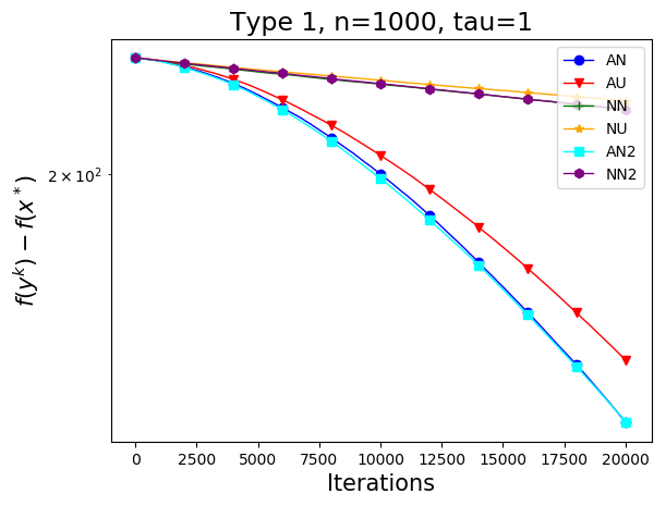
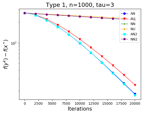
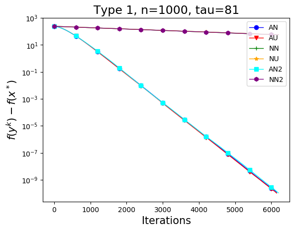
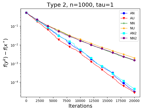
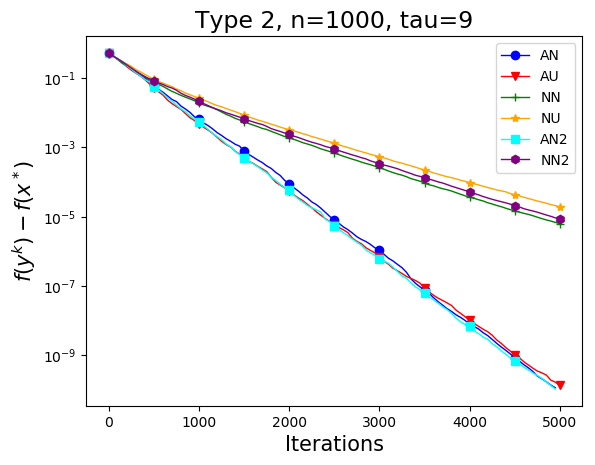
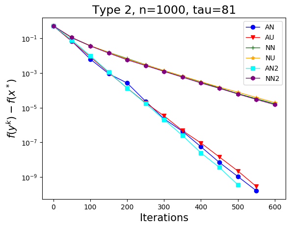
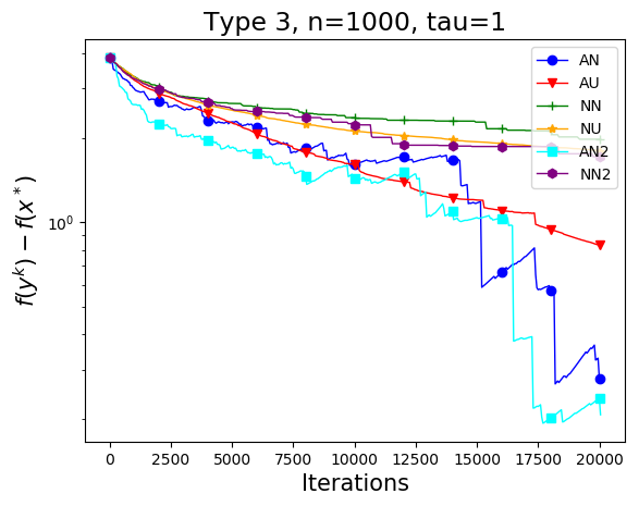
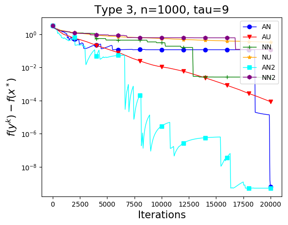
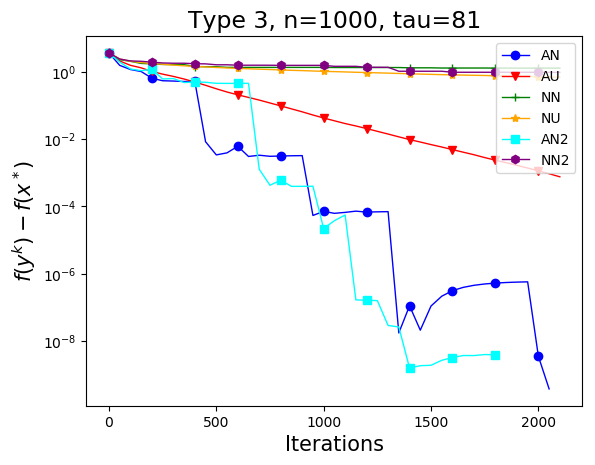
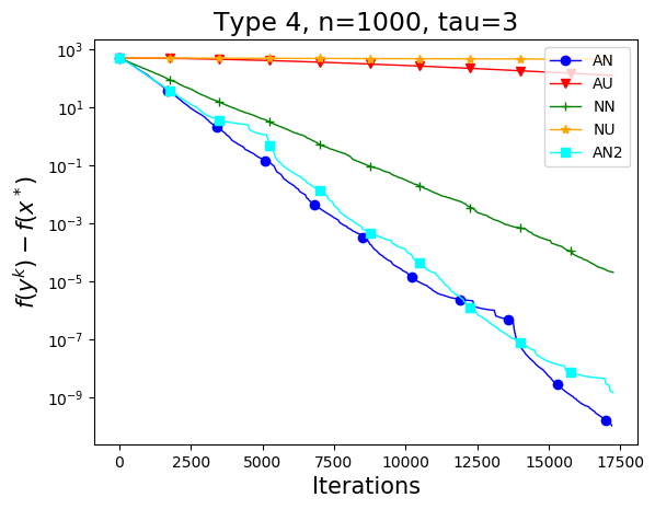
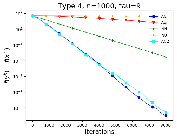
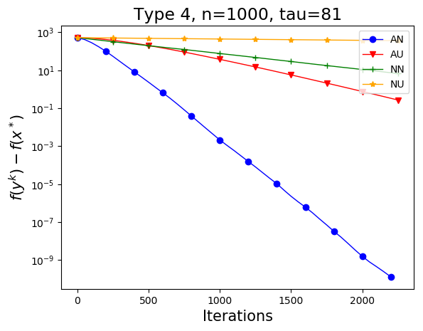
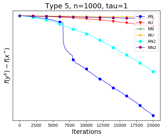
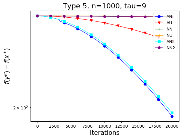
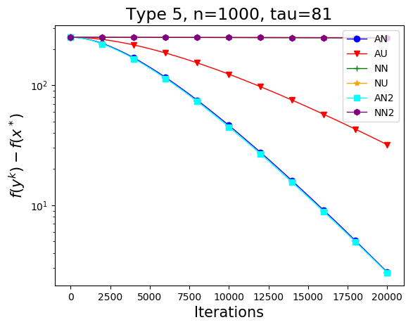
Figure 2: Comparison of accelerated, nonaccelerated algorithm with both importance and $\tau$ nice sampling for a various quadratic problems.

D.1.2 Speedup in $\tau$

The next experiment shows an empirical speedup for the coordinate descent algorithms for a various types of problems. For simplicity, we do not include Sampling 2. Figure 3 provides the results. Oftentimes, the empirical speedup (in terms of the number of iteration) in $\tau$ is close to linear, which demonstrates the power and significance of minibatching.

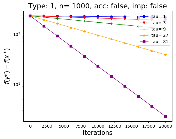
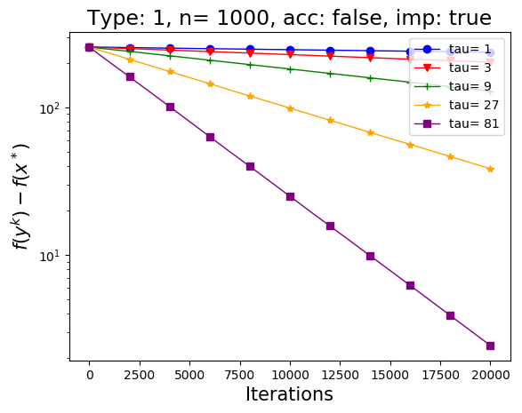
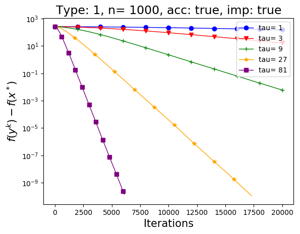
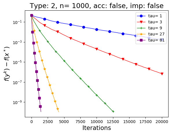
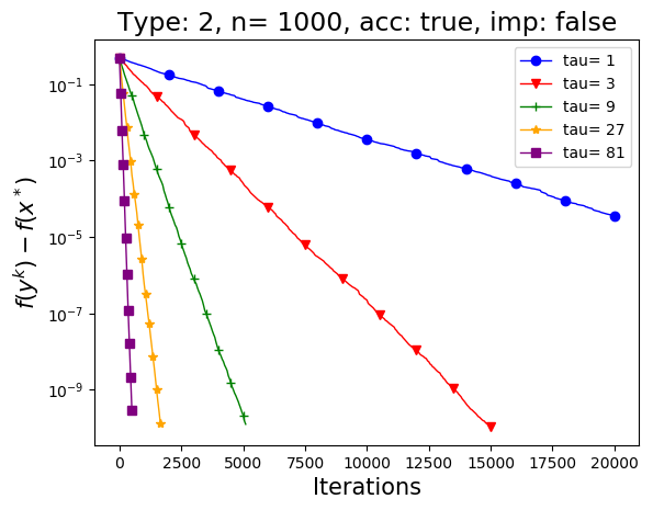
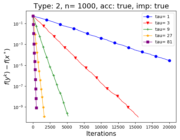
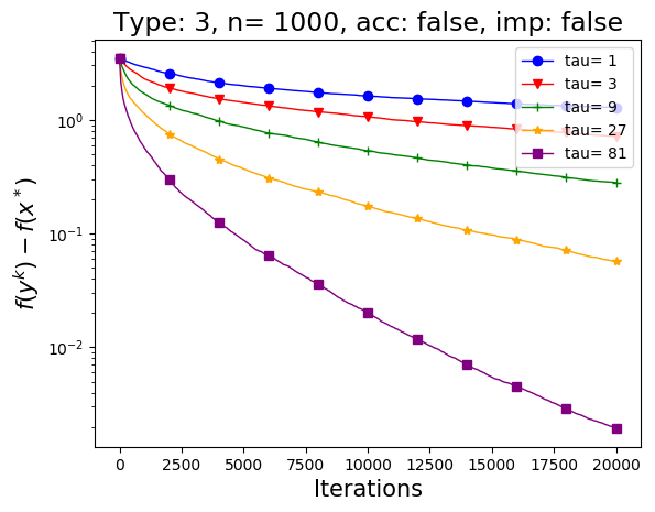
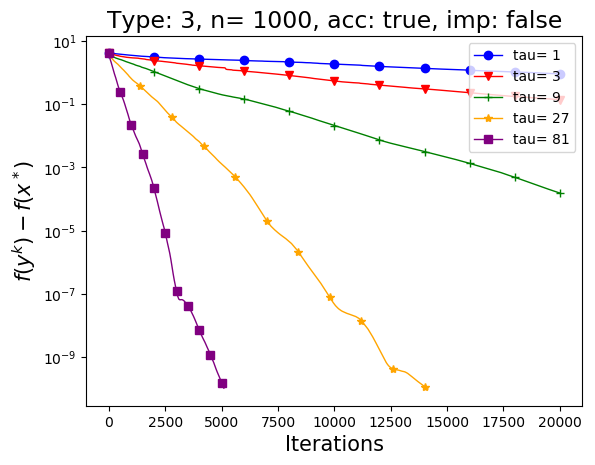
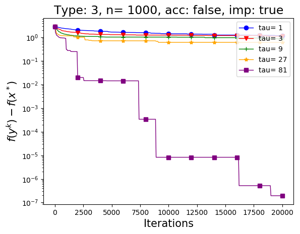
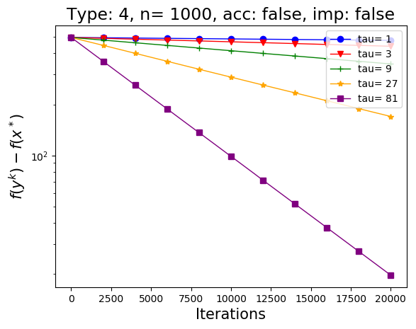
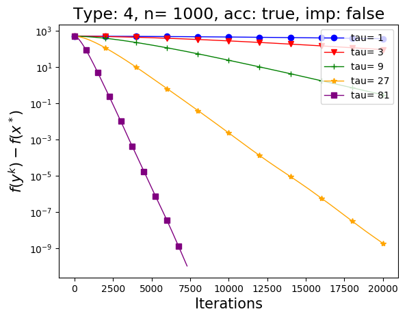
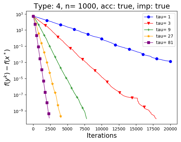
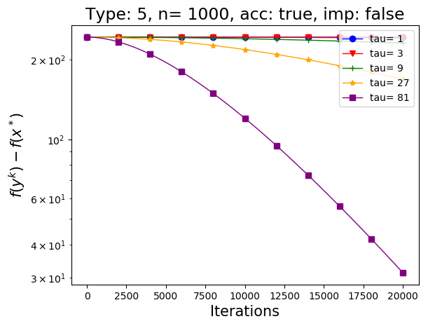
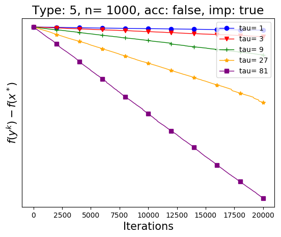
Figure 3: Comparison of speedup gained by both $\tau$-nice sampling and importance sampling with and without acceleration on various quadratic problems.

D.2 Logistic Regression

In this section we apply ACD on the regularized logistic regression problem, i.e.

$$f(x)=\frac{1}{m}\sum_{i=1}^{m}\log\left(1+\exp\left({\bf A}_{i,:}x\cdot b\right)\right)+\frac{\lambda}{2}\|x\|^{2},$$

for $b\in\{-1,1\}$ and data matrix ${\bf A}$ comes from LibSVM. In each experiment in this section, we have chosen regularization parameter $\lambda$ to be the average diagonal element of the smoothness matrix. We first apply the methods with the optimal parameters as our theory suggests on smaller datasets. On larger ones (Section D.2.1), we set them in a cheaper way, which is not guaranteed to work by theory we provide.

In our first experiment, we apply ACD on LibSVM data directly for various minibatch sizes $\tau$. Figure 4 shows the results. As expected, ACD is always better to CD, and importance sampling is always better to uniform one.

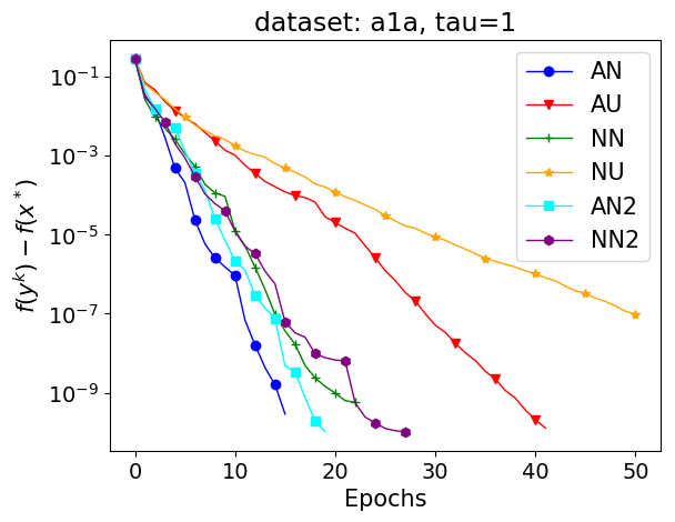
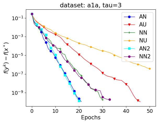
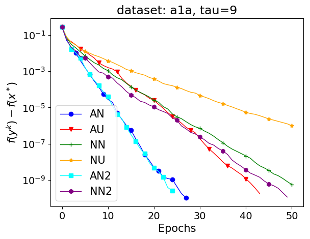
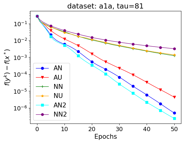
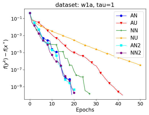
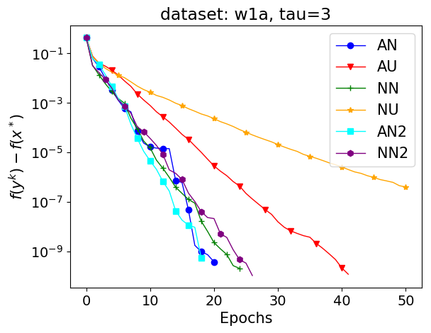
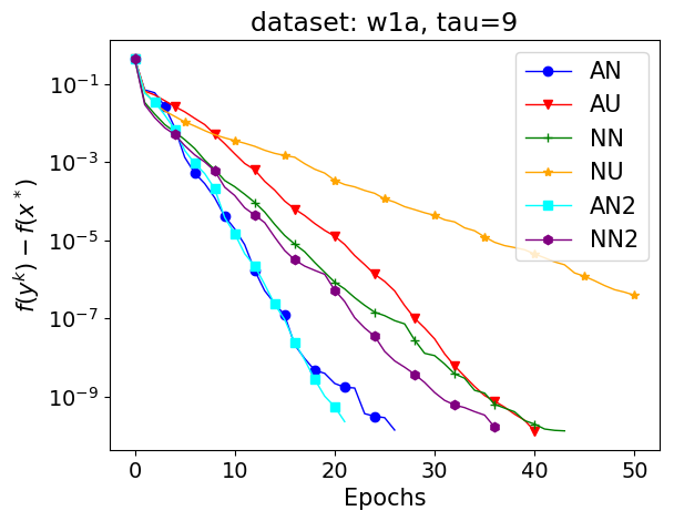
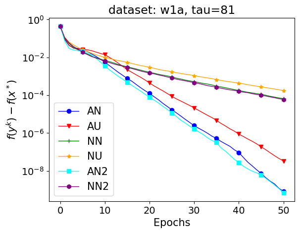
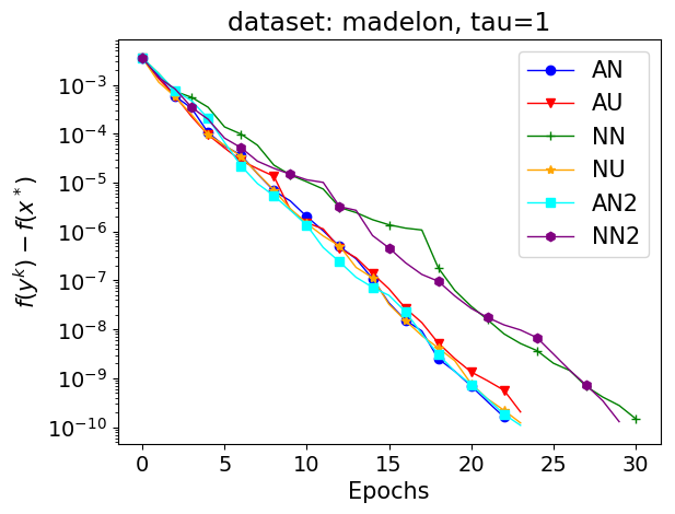
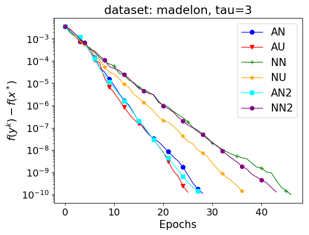
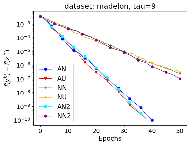
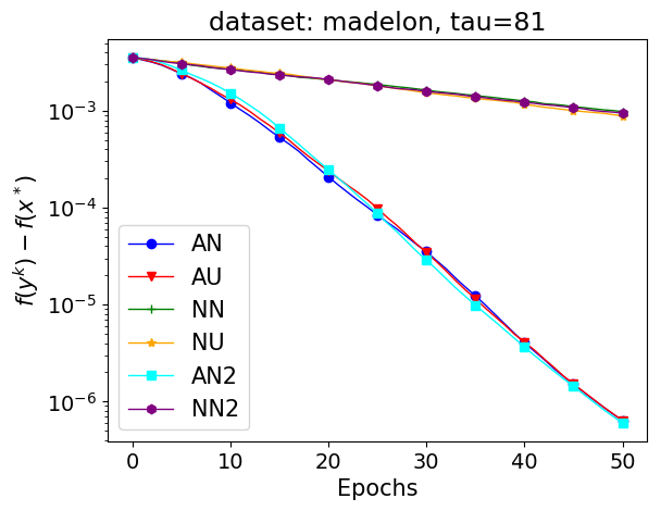
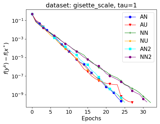
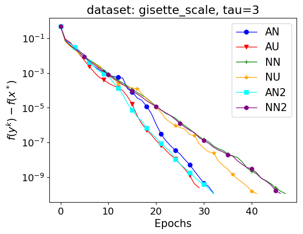
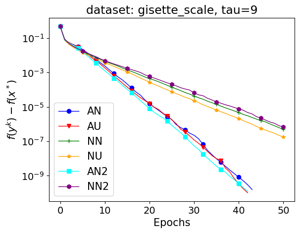
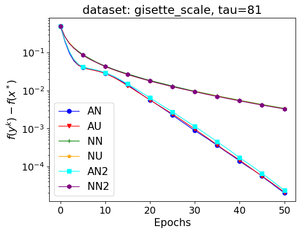
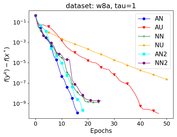
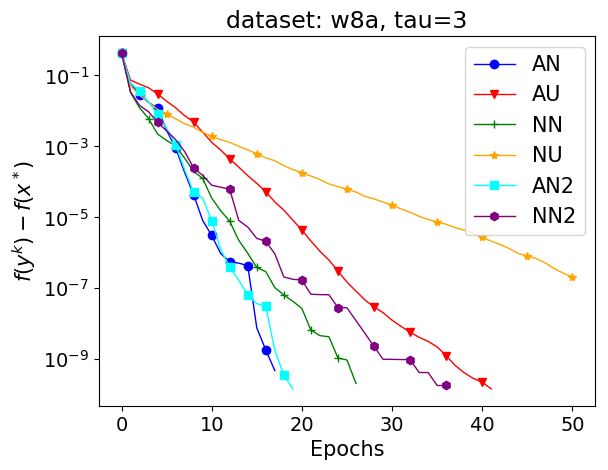
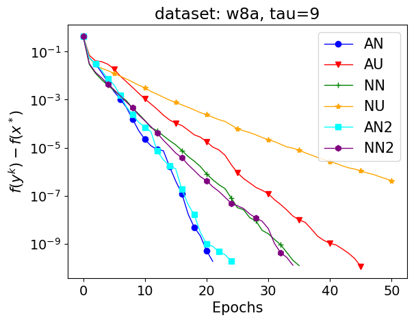
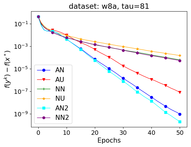
Figure 4: Accelerated coordinate desent applied on the logistic regression problem, for various LibSVM datasets and minibatch sizes $\tau$

Note that, for for some datasets and especially bigger minibatch sizes, the effect of importance sampling is sometimes negligible. To demonstrate the power of importance sampling, in the next experiment, we first corrupt the data – we multiply each row and column of the data matrix ${\bf A}$ by random number from uniform distribution over $[0,1]$. The results can be seen in Figure 5. As expected, the effect of importance sampling becomes more significant.

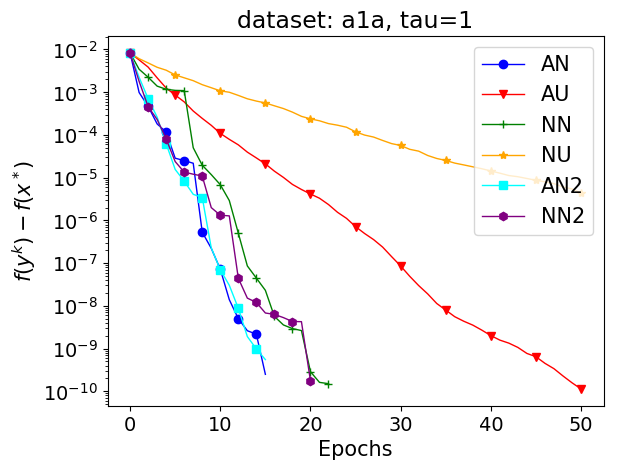
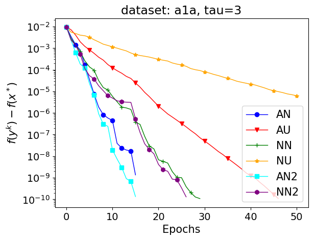
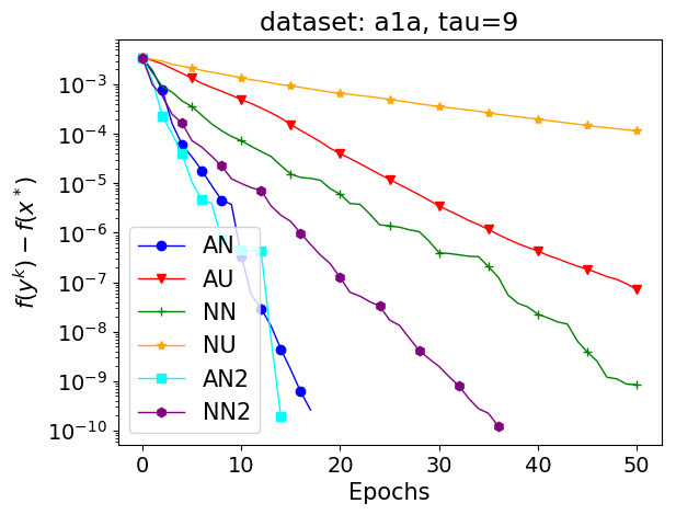
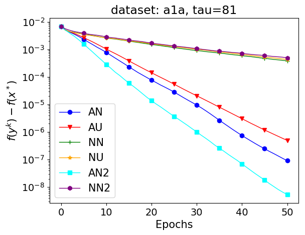
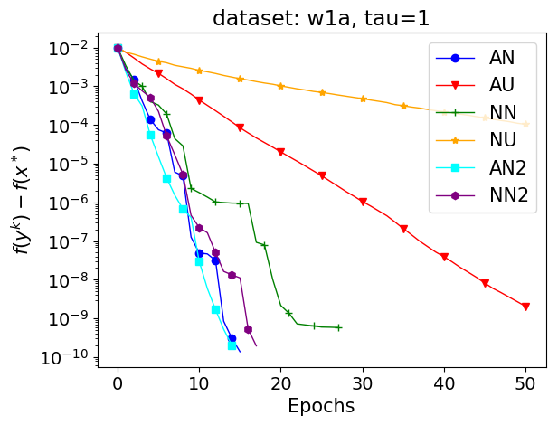
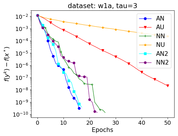
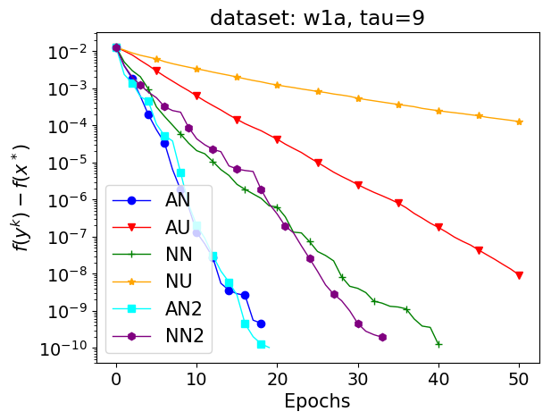
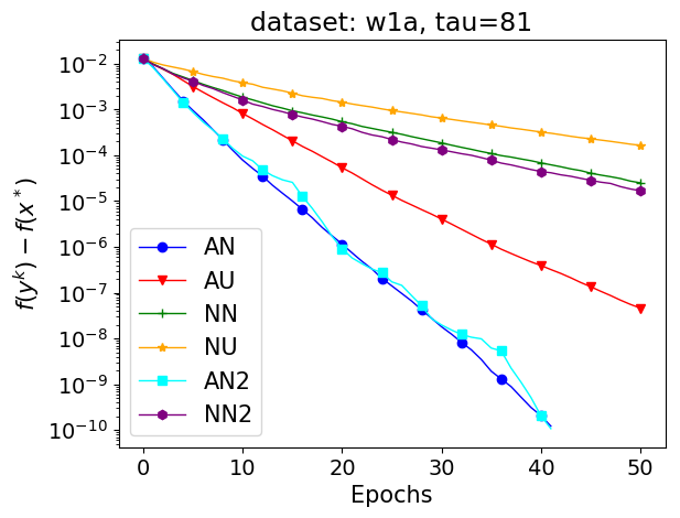
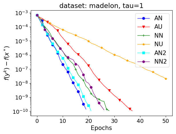
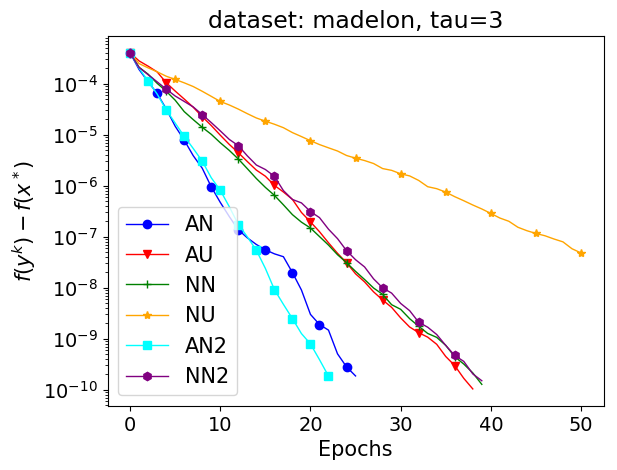
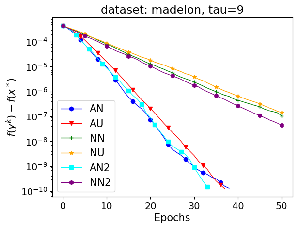
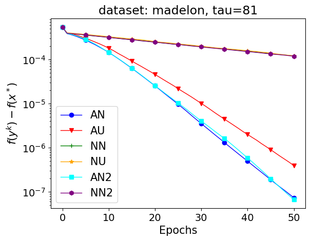
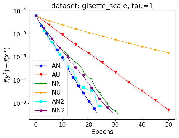
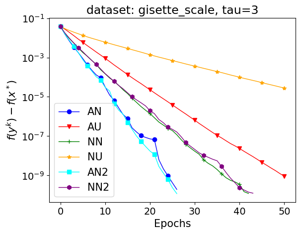
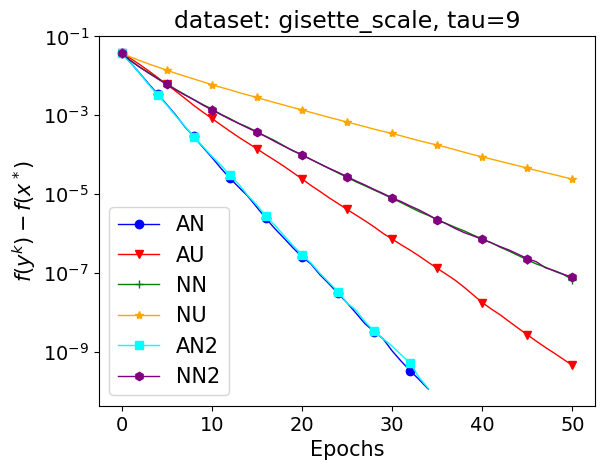
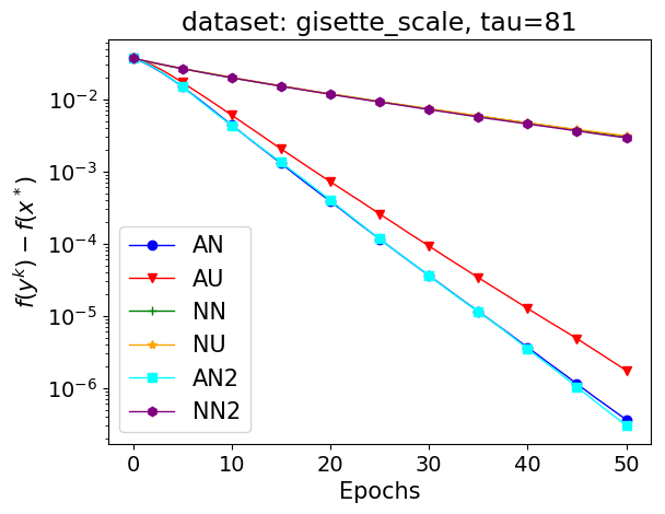
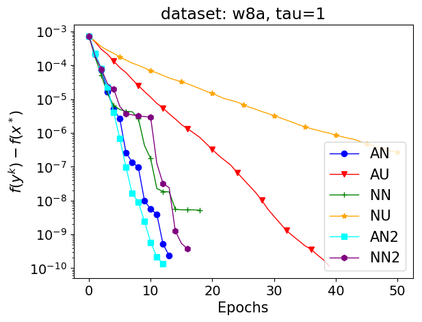
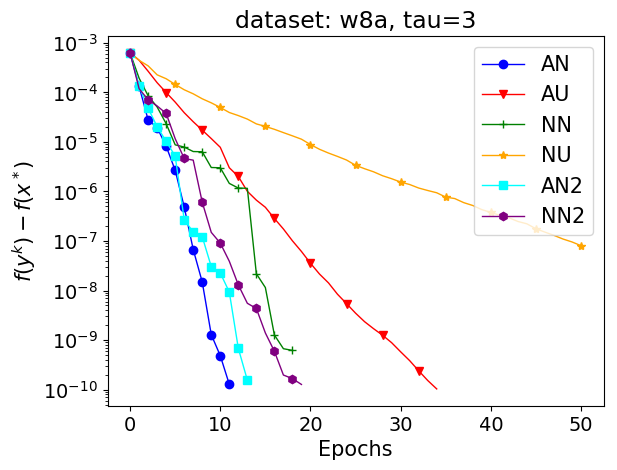
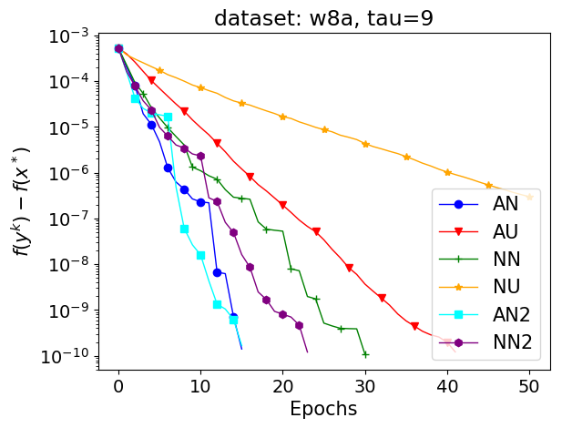
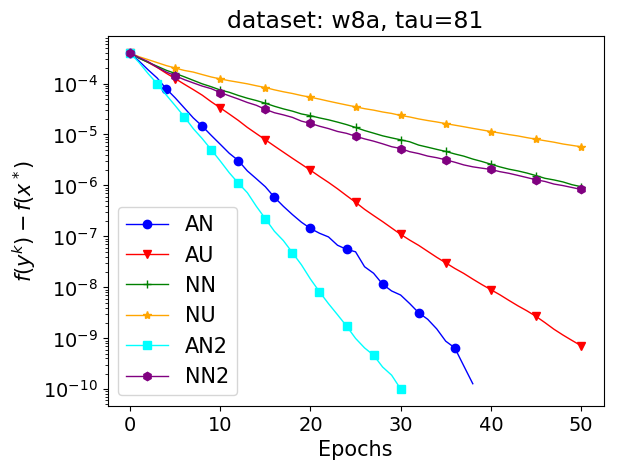
Figure 5: Accelerated coordinate desent applied on the logistic regression problem, for various rescaled LibSVM datasets and minibatch sizes $\tau$

D.2.1 Practical method on larger dataset

For completeness, we restate here experiments from Figure 1. We have chosen regularization parameter $\lambda$ to be the average diagonal element of the smoothness matrix and estimated $v,\sigma$ as described in Section 6.

Figure 6: Six variants of coordinate descent (AN, AU, NN, NU, AN2 and AU2) applied to a logistic regression problem, with minibatch sizes $\tau=1,8,64$ and $512$.

D.3 Support Vector Machines

In this section we apply ACD on the dual of SVM problem with squared hinge loss, i.e.,

$$f(x)=\frac{1}{\lambda n^{2}}\sum_{j=1}^{m}\left(\sum_{i=1}^{n}b_{i}{\bf A}_{ji}x_{i}\right)^{2}-\frac{1}{n}\sum_{i=1}^{n}x_{i}+\frac{1}{4n}\sum_{i=1}^{n}x_{i}^{2}+{\cal I}_{[0,\infty]}(x),$$

where ${\cal I}_{[0,\infty]}$ stands for indicator function of set $[0,\infty]$, i.e. ${\cal I}_{[0,\infty]}(x)=0$ if $x\in\mathbb{R}^{n}_{+}$, otherwise ${\cal I}_{[0,\infty]}(x)=\infty$. As for the data, we have rescaled each row and each column of the data matrix coming frol LibSVM by random scalar generated from uniform distribution over $[0,1]$. We have chosen regularization parameter $\lambda$ to be maximal diagonal element of the smoothness matrix divided by 10 in each experiment below. We deal with nonsmooth indicator function using proximal operator, which happens to be a projection in this case. We choose ESO parameters $v$ from Lemma 5.2, while estimating the smoothness matrix as $\sqrt{n}$–times multiple of its diagonal. An estimate of the strong convexity $\sigma$ for acceleration was chosen to be minimal diagonal element of the smoothness matrix, therefore we adapt a similar approach as in Section D.2.1.

Recall that we did not provide a theory for the proximal steps. However, we make the experiment to demonstrate that ACD can solve big data problems on top of large dimensional problems. The results (Figure 7) again suggests the great significance of the acceleration and importance sampling.

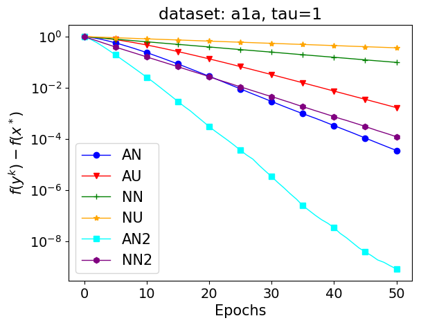
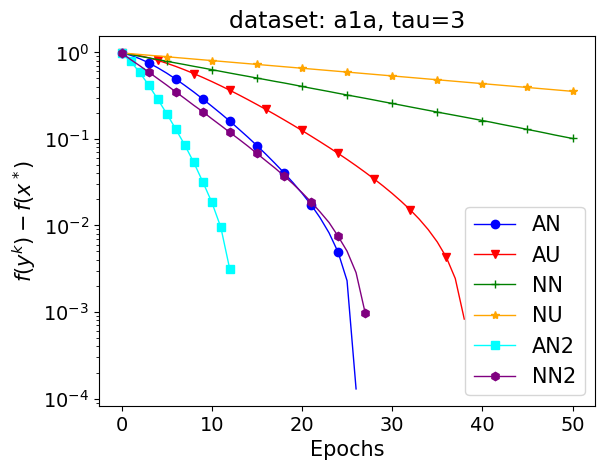
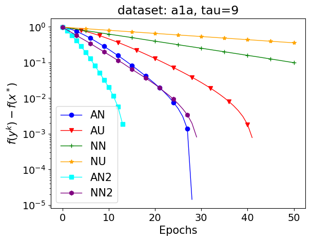
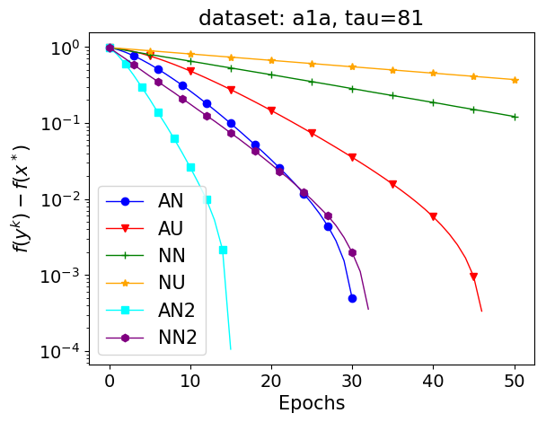
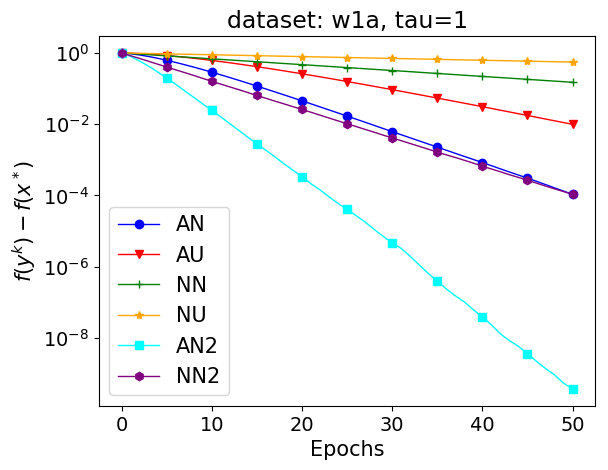
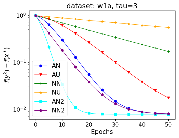
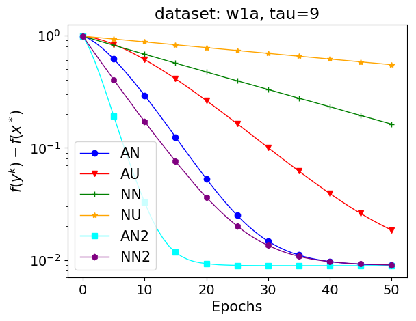
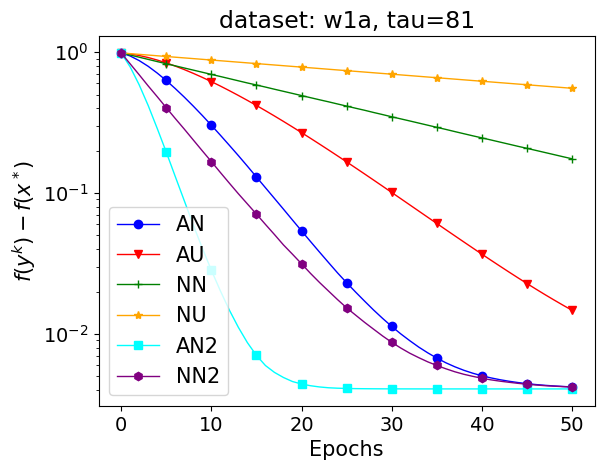
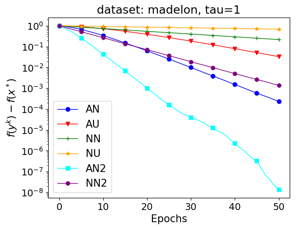
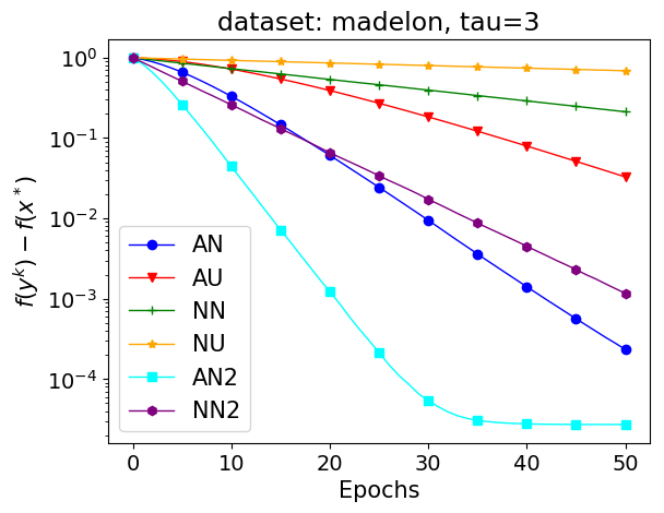
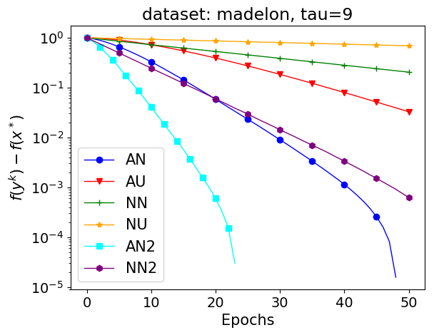
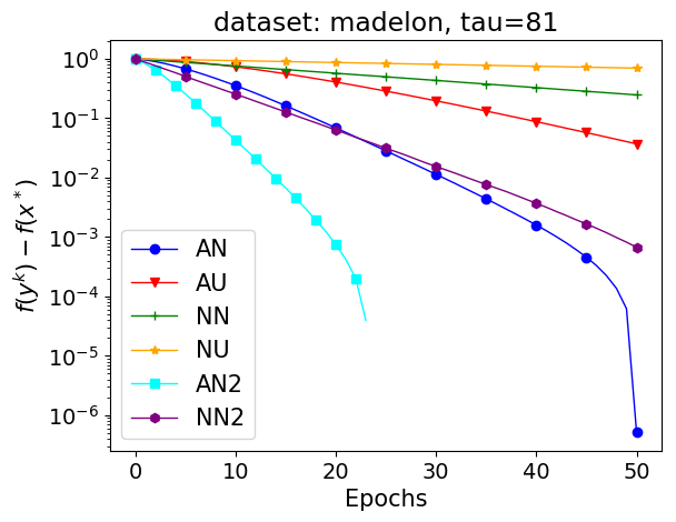
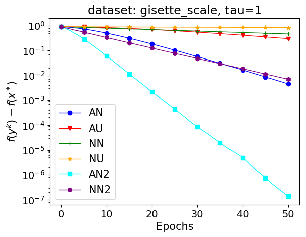
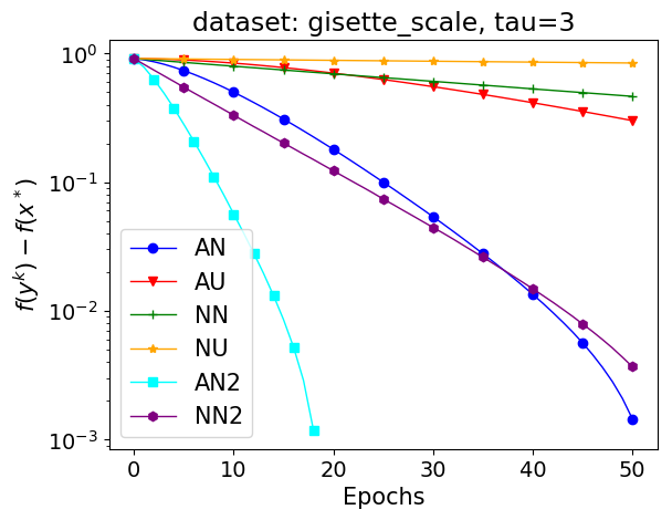
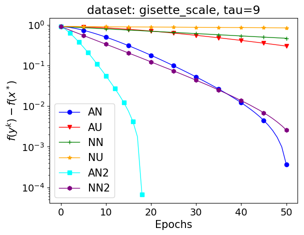
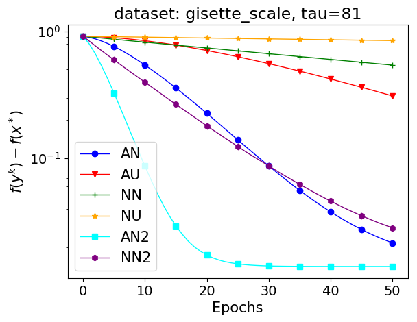
Figure 7: Accelerated coordinate desent applied on the dual of of SVM with squared hinge loss, for various LibSVM datasets

References

- [1] Zeyuan Allen-Zhu and Lorenzo Orecchia. Linear coupling: An ultimate unification of gradient and mirror descent. In Innovations in Theoretical Computer Science, 2017.
- [2] Zeyuan Allen-Zhu, Zheng Qu, Peter Richtarik, and Yang Yuan. Even faster accelerated coordinate descent using non-uniform sampling. In Proceedings of The 33rd International Conference on Machine Learning, volume 48 of Proceedings of Machine Learning Research, pages 1110–1119, New York, New York, USA, 2016.
- [3] Antonin Chambolle, Matthias J. Ehrhardt, Peter Richtárik, and Carola-Bibiane Schöenlieb. Stochastic primal-dual hybrid gradient algorithm with arbitrary sampling and imaging applications. arXiv:1706.04957, 2017.
- [4] Chih-Chung Chang and Chih-Jen Lin. LibSVM: A library for support vector machines. ACM Transactions on Intelligent Systems and Technology (TIST), 2(3):27, 2011.
- [5] Dominik Csiba, Zheng Qu, and Peter Richtarik. Stochastic dual coordinate ascent with adaptive probabilities. In Proceedings of the 32nd International Conference on Machine Learning, volume 37 of Proceedings of Machine Learning Research, pages 674–683, Lille, France, 2015.
- [6] Dominik Csiba and Peter Richtárik. Importance sampling for minibatches. Journal of Machine Learning Research, 19(27), 2018.
- [7] Olivier Fercoq, Zheng Qu, Peter Richtárik, and Martin Takáč. Fast distributed coordinate descent for minimizing non-strongly convex losses. IEEE International Workshop on Machine Learning for Signal Processing, 2014.
- [8] Olivier Fercoq and Peter Richtárik. Accelerated, parallel and proximal coordinate descent. SIAM Journal on Optimization, 25(4):1997–2023, 2015.
- [9] Mert Gurbuzbalaban, Asuman Ozdaglar, Pablo A Parrilo, and Nuri Vanli. When cyclic coordinate descent outperforms randomized coordinate descent. In Advances in Neural Information Processing Systems, pages 7002–7010, 2017.
- [10] Yin Tat Lee and Aaron Sidford. Efficient accelerated coordinate descent methods and faster algorithms for solving linear systems. Proceedings - Annual IEEE Symposium on Foundations of Computer Science, FOCS, pages 147–156, 2013.
- [11] Qihang Lin, Zhaosong Lu, and Lin Xiao. An accelerated proximal coordinate gradient method. In Advances in Neural Information Processing Systems, pages 3059–3067, 2014.
- [12] Zhi-Quan Luo and Paul Tseng. On the convergence of the coordinate descent method for convex differentiable minimization. Journal of Optimization Theory and Applications, 72(1):7–35, 1992.
- [13] Yu Nesterov. Efficiency of coordinate descent methods on huge-scale optimization problems. SIAM Journal on Optimization, 22(2):341–362, 2012.
- [14] Yurii Nesterov. A method of solving a convex programming problem with convergence rate . Soviet Mathematics Doklady, 27(2):372–376, 1983.
- [15] Yurii Nesterov. Introductory Lectures on Convex Optimization: A Basic Course (Applied Optimization). Kluwer Academic Publishers, 2004.
- [16] Yurii Nesterov. Efficiency of coordinate descent methods on huge-scale optimization problems. SIAM Journal on Optimization, 22(2):341–362, 2012.
- [17] Julie Nutini, Mark Schmidt, Issam Laradji, Michael Friedlander, and Hoyt Koepke. Coordinate descent converges faster with the Gauss-Southwell rule than random selection. In Proceedings of the 32nd International Conference on Machine Learning, volume 37 of Proceedings of Machine Learning Research, pages 1632–1641, Lille, France, 2015.
- [18] Zheng Qu and Peter Richtárik. Coordinate descent with arbitrary sampling I: Algorithms and complexity. Optimization Methods and Software, 31(5):829–857, 2016.
- [19] Zheng Qu and Peter Richtárik. Coordinate descent with arbitrary sampling II: Expected separable overapproximation. Optimization Methods and Software, 31(5):858–884, 2016.
- [20] Zheng Qu, Peter Richtárik, and Tong Zhang. Quartz: Randomized dual coordinate ascent with arbitrary sampling. In Advances in Neural Information Processing Systems 28, 2015.
- [21] Peter Richtárik and Martin Takáč. Distributed coordinate descent method for learning with big data. Journal of Machine Learning Research, 17(75):1–25, 2016.
- [22] Peter Richtárik and Martin Takáč. On optimal probabilities in stochastic coordinate descent methods. Optimization Letters, 10(6):1233–1243, 2016.
- [23] Peter Richtárik and Martin Takáč. Iteration complexity of randomized block-coordinate descent methods for minimizing a composite function. Mathematical Programming, 144(2):1–38, 2014.
- [24] Peter Richtárik and Martin Takáč. Parallel coordinate descent methods for big data optimization. Mathematical Programming, 156(1-2):433–484, 2016.
- [25] Ankan Saha and Ambuj Tewari. On the nonasymptotic convergence of cyclic coordinate descent methods. SIAM Journal on Optimization, 23(1):576–601, 2013.
- [26] Shai Shalev-Shwartz and Ambuj Tewari. Stochastic methods for l1-regularized loss minimization. Journal of Machine Learning Research, 12(Jun):1865–1892, 2011.
- [27] Shai Shalev-Shwartz and Tong Zhang. Stochastic dual coordinate ascent methods for regularized loss. Journal of Machine Learning Research, 14(1):567–599, 2013.
- [28] Shai Shalev-Shwartz and Tong Zhang. Accelerated proximal stochastic dual coordinate ascent for regularized loss minimization. In Proceedings of the 31st International Conference on Machine Learning, volume 32 of Proceedings of Machine Learning Research, pages 64–72, Bejing, China, 2014.
- [29] Sebastian U. Stich, Anant Raj, and Martin Jaggi. Approximate steepest coordinate descent. In Proceedings of the 34th International Conference on Machine Learning, volume 70 of Proceedings of Machine Learning Research, pages 3251–3259, International Convention Centre, Sydney, Australia, 2017.
- [30] Sebastian U Stich, Anant Raj, and Martin Jaggi. Safe adaptive importance sampling. In Advances in Neural Information Processing Systems, pages 4384–4394, 2017.
- [31] Paul Tseng. Convergence of a block coordinate descent method for nondifferentiable minimization. Journal of Optimization Theory and Applications, 109(3):475–494, 2001.
- [32] Stephen J Wright. Coordinate descent algorithms. Mathematical Programming, 151(1):3–34, 2015.
- [33] Yang You, Xiangru Lian, Ji Liu, Hsiang-Fu Yu, Inderjit S Dhillon, James Demmel, and Cho-Jui Hsieh. Asynchronous parallel greedy coordinate descent. In Advances in Neural Information Processing Systems, pages 4682–4690, 2016.
- [34] Fuzhen Zhang. Matrix Theory: Basic Results and Techniques. Springer-Verlag New York, 1999.
- [35] Peilin Zhao and Tong Zhang. Stochastic optimization with importance sampling for regularized loss minimization. In Proceedings of the 32nd International Conference on Machine Learning, volume 37 of Proceedings of Machine Learning Research, pages 1–9, Lille, France, 2015.