Quantum fluctuations of a resonantly interacting $p$-wave Fermi superfluid in two dimensions

Abstract

Using the Gaussian pair fluctuation theory, we investigate quantum fluctuations of a strongly interacting two-dimensional chiral p-wave Fermi superfluid at the transition from a Bose-Einstein condensate (BEC) to a topologically non-trivial Bardeen-Cooper-Schrieffer (BCS) superfluid. Near the topological phase transition at zero chemical potential, $\mu=0$, we observe that quantum fluctuations strongly renormalize the zero-temperature equations of state, sound velocity, pair-breaking velocity, and Berezinskii-Kosterlitz-Thouless (BKT) critical temperature of the Fermi superfluid, all of which can be non-analytic functions of the interaction strength. The indication of non-analyticity is particularly evident in the BKT critical temperature, which also exhibits a pronounced peak near the topological phase transition. Across the transition and towards the BEC limit we find that the system quickly becomes a trivial interacting Bose liquid, whose properties are less dependent on the interparticle interaction. The qualitative behavior of composite bosons in the BEC limit remains to be understood.

I Introduction

Unconventional electronic superconductivity and fermionic superfluidity are of great interest and lie at the heart of many intriguing quantum materials Mineev1999 . One of the most important examples is the two-dimensional (2D) chiral $p$-wave superconductor (superfluid), where the pairing order parameter has the $p_{x}+ip_{y}$ symmetry in its orbital angular momentum. It was shown to be topologically non-trivial with vortex excitations that exhibit non-Abelian statistics Read2000 ; Ivanov2001 . These so-called Majorana excitations have been suggested to be a key ingredient for processing topological quantum computation Kitaev2003 ; Nayak2008 . Unfortunately, in spite of extensive search for decades, a 2D $p$-wave superconductor remains elusive in condensed matter physics. The best-known candidate material of 2D $p$-wave superconductors so far is strontium ruthenate Sr₂RuO₄, whose superconductivity was first observed by Maeno and his group in 1994 Maeno1994 .

The recent realization of resonantly interacting ultracold atomic Fermi gases opens a new paradigm to create the topological $p$-wave superfluid Gurarie2007 . By tuning the $s$-wave interparticle interaction in a two-component Fermi gas through magnetic Feshbach resonances, the crossover from a Bardeen-Cooper-Schrieffer (BCS) fermionic superfluid to a Bose-Einstein condensate (BEC) has now been routinely observed in laboratories Bloch2008 ; Giorgini2008 , confirming the long-sought BEC-BCS crossover Eagles1969 ; Leggett1980 ; Nozieres1985 ; SadeMelo1993 in both three and two dimensions. A resonantly interacting $p$-wave Fermi gas can be realized by either using $p$-wave Feshbach resonances or by preparing fermionic atoms in the same hyperfine pseudo-spin state, which experience long-range dipole-dipole interactions. The former has already been demonstrated for ⁴⁰K and ⁶Li atoms Regal2003 ; Zhang2004 ; Gunter2005 ; Schunck2005 ; Gaebler2007 ; Fuchs2008 ; Inada2008 ; Nakasuji2013 ; Luciuk2016 ; Waseem2017 ; Yoshida2018 ; Wassem2018 , although the system suffers a serious loss in atom number near the $p$-wave resonance. Nevertheless, in three dimensions the system can still reach a quasi-equilibrium state Luciuk2016 , in which a number of interesting physical properties of the cloud can be experimentally examined. More importantly, in lower dimensions the atom loss has been found to be significantly reduced Waseem2017 , as theoretically predicted Levinsen2008 ; Fedorov2017 . For a single-component dipolar Fermi gas Lu2012 ; Aikawa2014 the $s$-wave scattering is completely suppressed by Pauli exclusion principle. The $p$-wave component of the interparticle interaction could then be significantly enhanced by suitably tuning the strength of the dipole-dipole interaction. All these recent experimental advances in ultracold atoms make the realization of a 2D $p$-wave Fermi superfluid a very appealing idea.

Theoretically, the many-body physics of strongly interacting $p$-wave Fermi gases has been studied to some extent Gurarie2007 . These include the exploration of the phase diagram Botelho2005 ; Ho2005 ; Gurarie2005 ; Cheng2005 ; Iskin2006 ; Cao2013 , which becomes richer due to the anisotropy in the different $p$-wave channels, determining the transition temperature for the superfluid transition in three dimensions Ohashi2005 ; Inotani2012 ; Inotani2015 or the Berezinskii-Kosterlitz-Thouless (BKT) transition in two dimensions Cao2017 , as well as the calculation of the $p$-wave contact parameters Yoshida2015 ; Yu2015 ; He2016 ; Peng2016 ; Zhang2017 ; Yao2018 ; Inotani2018 , which characterize the universal short-distance and large-momentum behavior of the system Tan2008 ; Braaten2008 . Most of these theoretical investigations rely on the mean-field theory, which qualitatively captures the underlying physics of the $p$-wave pairing. To describe more accurately a $p$-wave Fermi superfluid, in particular in two dimensions, it is necessary to include strong quantum fluctuations beyond mean-field close to the resonantly interacting regime Liu2018 ; Jiang2018 . In this respect, it is convenient to adopt the Gaussian pair fluctuation (GPF) theory Hu2006 ; Diener2008 , which provides a quantitatively reliable description of an $s$-wave Fermi superfluid at the BEC-BCS crossover, in both three Hu2006 ; Hu2007 ; Diener2008 and two dimensions He2015 .

In this work, we explore quantum fluctuations in a 2D chiral $p$-wave Fermi superfluid using the GPF theory, paying specific attention to the role played by the topological phase transition at zero chemical potential. A number of physical observables at zero temperature are considered across the BEC-BCS transition, such as the chemical potential, total energy, pressure equation of state, sound velocity, pair-breaking velocity, and also the critical velocity for superfluidity. All these quantities are strongly affected by quantum fluctuations. By assuming the existence of well-defined fermionic Bogoliubov quasi-particles and bosonic excitations of phonons, we further calculate the temperature dependence of superfluid fraction with the approximate Landau formalism Bighin2016 . This leads to an improved determination of the BKT critical temperature in the strongly interacting regime.

The paper is organized as follows. In the next section (Sec. II), we present the model Hamiltonian of a 2D spin-less $p$-wave interacting Fermi gas. In Sec. III, we describe the details of the GPF theory of the chiral $p$-wave Fermi superfluid. In Sec. IV, we first discuss various equations of state as a function of the interaction strength, including the chemical potential, pressure, and total energy. We then present the results of sound velocity, pair-breaking velocity, and critical velocity. Based on the single-particle fermionic excitation spectrum and the sound velocity at zero temperature, we calculate the temperature dependence of superfluid density within the Landau picture for superfluidity and consequently determine the BKT critical temperature. Finally, in Sec. VI we give our conclusions and outlook.

II Model Hamiltonian

We consider a spin-less 2D atomic Fermi gas of density $n$, interacting in the dominant $p$-wave channel near a broad $p$-wave Feshbach resonance, as described by a single-channel Hamiltonian (we set the area $A=1$) Botelho2005 ,

$${\cal H}=\sum_{{\bf k}}\xi_{{\bf k}}\psi_{{\bf k}}^{\dagger}\psi_{{\bf k}}+\frac{1}{2}\sum_{{\bf k},{\bf k}^{\prime},{\bf q}}V_{\mathbf{k}\mathbf{k}^{\prime}}b_{\mathbf{k}\mathbf{q}}^{\dagger}b_{\mathbf{k^{\prime}}\mathbf{q}},$$ (1)

where $\psi_{{\bf k}}$ ($\psi_{{\bf k}}^{\dagger}$) is the annihilation (creation) field operator for atoms with mass $M$ and the single-particle dispersion $\xi_{{\bf k}}\equiv\epsilon_{{\bf k}}-\mu=\hbar^{2}\mathbf{k}^{2}/(2M)-\mu$, and $b_{\mathbf{k}\mathbf{q}}\equiv\psi_{-{\bf k}{\bf+q}/2}\psi_{{\bf k}{\bf+q}/2}$ is the composite operator that annihilates a pair of atoms with a center-of-mass momentum $\mathbf{q}$. We work with the grand-canonical ensemble and tune the chemical potential $\mu$ to make the average density

$$\sum_{\mathbf{k}}\left\langle\hat{n}_{{\bf k}}\right\rangle=n\equiv\frac{k_{F}^{2}}{4\pi},$$ (2)

where $\hat{n}_{\mathbf{k}}\equiv\psi_{{\bf k}}^{\dagger}\psi_{{\bf k}}$ and $k_{F}$ is the Fermi wave-vector. For the inter-particle interaction, we adopt the following separable form Nozieres1985 ; Botelho2005 ; Ho2005 ,

$$V_{\mathbf{k}\mathbf{k}^{\prime}}=\lambda\Gamma\left({\bf k}\right)\Gamma^{*}\left({\bf k^{\prime}}\right),$$ (3)

where $\lambda<0$ is the bare interaction strength and the dimensionless regularization function $\Gamma\left({\bf k}\right)$ represents the chiral $p_{x}+ip_{y}$ symmetry of the pairing interaction, i.e.,

$$\Gamma\left({\bf k}\right)=\frac{\left(k/k_{F}\right)}{\left[1+\left(k/k_{0}\right)^{2n}\right]^{3/2}}e^{i\varphi_{{\bf k}}}.$$ (4)

Here, $k_{0}$ is a large momentum cut-off, which is necessary to make the model Hamiltonian renormalizable, and $\varphi_{{\bf k}}$ is the polar angle of ${\bf k}$. We use the exponent $n$ to tune the shape of the regularization function $\Gamma\left({\bf k}\right)$ and to confirm the insensitivity of our results on the form of the interparticle interaction. The choice of $n=1/2$ was used earlier by Noziéres and Schmitt-Rink Nozieres1985 , and Botelho and Sá de Melo Botelho2005 . In this paper, unless otherwise specified, we follow the work by Ho and Diener Ho2005 and take $n=1$ for the numerical results presented. Actually, the results depend very weakly on the exponent $n$. The use of other values of $n$ only leads to small quantitative difference.

In principle, the bare interaction strength $\lambda$ and the cut-off momentum $k_{0}$ should be renormalized (i.e., replaced) in terms of the 2D $p$-wave scattering area $a_{p}$ and effective range $R_{p}\sim 1/k_{0}$ Zhang2017 . However, for a better presentation, it turns out to be more convenient to use a scattering energy $E_{b}$ Botelho2005 ; Cao2017 , which is basically the ground state energy of two fermions at zero center-of-mass momentum,

$$2\epsilon_{{\bf k}}\psi_{{\bf k}}+\sum_{{\bf k}^{\prime}}V_{{\bf kk}^{\prime}}\psi_{{\bf k}^{\prime}}=E_{b}\psi_{{\bf k}}.$$ (5)

By inserting the separable interaction potential, it is easy to obtain,

$$\frac{1}{\lambda}=-\sum_{{\bf k}}\frac{\left|\Gamma\left({\bf k}\right)\right|^{2}}{2\epsilon_{{\bf k}}-E_{b}}.$$ (6)

We note that, unlike the $s$-wave scattering in 2D, where the scattering energy $E_{b}$ is always negative, in our $p$-wave case $E_{b}$ can be either negative or positive. A negative scattering energy indicates the existence of a two-body bound state (i.e., on the BEC side), with a binding energy $\varepsilon_{B}=-E_{b}>0$. On the other hand, the weakly interacting BCS limit is reached at $E_{b}\rightarrow+\infty$. Throughout the paper, we use the set of parameters ($E_{b},k_{0},n=1$) to characterize the $p$-wave interaction. Their relation to the $p$-wave scattering area $a_{p}$ and effective range $R_{p}$ is briefly discussed in Appendix A.

III Gaussian pair function theory at zero temperature

In the superfluid phase at zero temperature, it is useful to introduce the Nambu spinor presentation for the field operators Hu2006 ; Diener2008 ,

$$\Psi_{{\bf k}}=\left(\begin{array}[]{l}\psi_{{\bf k}}\\ \psi_{-{\bf k}}^{\dagger}\end{array}\right),$$ (7)

with which, the model Hamiltonian can be rewritten as,

$${\cal H}=\frac{1}{2}\sum_{{\bf k}}\Psi_{{\bf k}}^{\dagger}\left(\xi_{{\bf k}}\sigma_{z}\right)\Psi_{{\bf k}}+\frac{1}{2\lambda}\sum_{{\bf q}}\hat{\rho}_{\mathbf{q}}^{\dagger}\hat{\rho}_{\mathbf{q}},$$ (8)

where

$$\hat{\rho}_{\mathbf{q}}\equiv\lambda\sum_{{\bf k}}\Gamma^{*}\left({\bf k}\right)b_{\mathbf{kq}}=\lambda\sum_{{\bf k}}\Psi_{{\bf k-\frac{q}{2}}}^{\dagger}\Gamma^{*}\left({\bf k}\right)\sigma_{-}\Psi_{{\bf k+\frac{q}{2}}}$$ (9)

is a generalized density operator for a pair of fermions and, $\sigma_{z}$ and $\sigma_{\pm}=(\sigma_{x}\pm\sigma_{y})/2$ are the Pauli matrices. In the following, we first solve the model Hamiltonian at the mean-field level and then include Gaussian pair fluctuations on top of the mean-field solution.

III.1 Mean-field theory

The superfluid phase is characterized by a nonzero (real) pairing order parameter $\Delta$ at zero center-of-mass momentum $\mathbf{q}=0$, i.e.,

$$\hat{\rho}_{\mathbf{q}}=\Delta\delta_{\mathbf{q},\mathbf{0}}+\Delta_{\mathbf{q}},$$ (10)

where $\Delta_{\mathbf{q}}$ is the pair fluctuation field around the order parameter. Inserting this decoupling into the model Hamiltonian, we obtain

$$\mathscr{\mathcal{H}} = \mathcal{H}_{\textrm{MF}}+\frac{1}{2\lambda}\sum_{{\bf q\neq 0}}\Delta_{\mathbf{q}}^{\dagger}\Delta_{\mathbf{q}},$$ (11)

$$\mathcal{H}_{\textrm{MF}} = \frac{1}{2}\sum_{{\bf k}}\Psi_{{\bf k}}^{\dagger}\left[\begin{array}[]{cc}\xi_{{\bf k}}&\Delta\Gamma\left({\bf k}\right)\\ \Delta\Gamma^{*}\left({\bf k}\right)&-\xi_{{\bf k}}\end{array}\right]\Psi_{{\bf k}}-\frac{\Delta^{2}}{2\lambda}.$$ (14)

Here, we neglect the fluctuation field at zero momentum, which gives a vanishing contribution in the thermodynamic limit. The mean-field Hamiltonian can be straightforwardly solved by diagonalizing the two by two matrix in Eq. (14). This leads to the following energy of Bogoliubov quasi-particles,

$$E_{{\bf k}}=\sqrt{\xi_{{\bf k}}^{2}+\Delta^{2}\left|\Gamma\left({\bf k}\right)\right|^{2}},$$ (15)

and quasi-particle wave-functions,

$$\left|u_{{\bf k}}\right|^{2} = \frac{1}{2}\left(1+\frac{\xi_{{\bf k}}}{E_{{\bf k}}}\right),$$ (16)

$$\left|v_{{\bf k}}\right|^{2} = \frac{1}{2}\left(1-\frac{\xi_{{\bf k}}}{E_{{\bf k}}}\right),$$ (17)

$$u_{{\bf k}}v_{{\bf k}}^{*} = \frac{\Delta\Gamma\left({\bf k}\right)}{2E_{{\bf k}}}.$$ (18)

The BCS Green function

$${\cal G}_{0}\left({\bf k},i\omega_{m}\right)=\left[\begin{array}[]{ll}i\omega_{m}-\xi_{{\bf k}}&-\Delta\Gamma\left({\bf k}\right)\\ -\Delta\Gamma^{*}\left({\bf k}\right)&i\omega_{m}+\xi_{{\bf k}}\end{array}\right]^{-1},$$ (19)

where $\omega_{m}=(2m+1)\pi k_{B}T$ ($m\in\mathbb{Z}$) is the fermionic Matsubara frequency, is then given by,

$${\cal G}_{0}^{11}\left({\bf k},i\omega_{m}\right) = \frac{u_{{\bf k}}u_{{\bf k}}^{*}}{i\omega_{m}-E_{{\bf k}}}+\frac{v_{{\bf k}}v_{{\bf k}}^{*}}{i\omega_{m}+E_{{\bf k}}},$$ (20)

$${\cal G}_{0}^{12}\left({\bf k},i\omega_{m}\right) = \frac{u_{{\bf k}}v_{{\bf k}}^{*}}{i\omega_{m}-E_{{\bf k}}}-\frac{u_{{\bf k}}v_{{\bf k}}^{*}}{i\omega_{m}+E_{{\bf k}}},$$ (21)

$${\cal G}_{0}^{21}\left({\bf k},i\omega_{m}\right) = \frac{u_{{\bf k}}^{*}v_{{\bf k}}}{i\omega_{m}-E_{{\bf k}}}-\frac{u_{{\bf k}}^{*}v_{{\bf k}}}{i\omega_{m}+E_{{\bf k}}},$$ (22)

$${\cal G}_{0}^{22}\left({\bf k},i\omega_{m}\right) = \frac{v_{{\bf k}}v_{{\bf k}}^{*}}{i\omega_{m}-E_{{\bf k}}}+\frac{u_{{\bf k}}u_{{\bf k}}^{*}}{i\omega_{m}+E_{{\bf k}}}.$$ (23)

The pairing order parameter can be determined by minimizing the mean-field thermodynamic potential,

$$\Omega_{\text{MF}} = \frac{1}{2}\frac{\Delta^{2}}{\lambda}+\frac{1}{2}\sum_{{\bf k}}\left(\xi_{{\bf k}}-E_{{\bf k}}\right),$$ (24)

$$= \frac{1}{2}\sum_{{\bf k}}\left[\xi_{{\bf k}}-E_{{\bf k}}-\frac{\Delta^{2}\left|\Gamma\left({\bf k}\right)\right|^{2}}{2\epsilon_{{\bf k}}-E_{b}}\right].$$

Thus, we obtain the gap equation,

$$\sum_{{\bf k}}\left[\frac{1}{2E_{{\bf k}}}-\frac{1}{2\epsilon_{{\bf k}}-E_{b}}\right]\left|\Gamma\left({\bf k}\right)\right|^{2}=0.$$ (25)

At the mean-field level, as mentioned earlier, the chemical potential $\mu$ is adjusted to satisfy the mean-field number equation,

$$n=n_{F}\equiv-\frac{\partial\Omega_{\text{MF}}}{\partial\mu}=\frac{1}{2}\sum_{{\bf k}}\left(1-\frac{\xi_{{\bf k}}}{E_{{\bf k}}}\right).$$ (26)

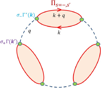
Figure 1: (color online). The third order ladder diagram considered in the Gaussian pair fluctuation theory. The solid line with arrow represents the two by two BCS Green functions. The dashed line with two vertices indicates the interparticle interaction. There are four types of ladders, $\Pi_{ss^{\prime}}$, depending on the choice of the interaction vertex: $s=+$ for $\sigma_{+}\Gamma(\mathbf{k}^{\prime})$ and $s=-$ for $\sigma_{-}\Gamma^{*}(\mathbf{k})$.

III.2 Gaussian pair fluctuation theory

We now take into account the fluctuation terms $\Delta_{\mathbf{q}}^{\dagger}\Delta_{\mathbf{q}}/(2\lambda)$ at nonzero center-of-mass momentum. At the lowest Gaussian level, their contribution to the thermodynamic potential can be represented by the ladder (or bubble) diagrams Nozieres1985 ; Hu2006 , one of which (i.e., the third order diagram) is shown in Fig. 1, where the dashed lines denote the bare interaction $\lambda\Gamma({\bf k)}\Gamma^{*}({\bf k^{\prime}})$. Following the standard diagrammatic rules Abrikosov1963 , a $n$-th order ladder diagram gives the following contribution to the thermodynamic potential,

$$\Omega_{\text{GF}}^{(n)} = \frac{\left(-1\right)^{n+1}\lambda^{n}}{2n}\sum_{\mathcal{Q}}\sum_{s_{1},\cdots,s_{n}^{\prime}}\left[\Pi\left(\mathcal{Q}\right)\right]_{s_{1}s_{1}^{\prime}}\cdots\left[\Pi\left(\mathcal{Q}\right)\right]_{s_{n}s_{n}^{\prime}},$$ (29)

$$= \frac{\left(-1\right)^{n+1}\lambda^{n}}{2n}\sum_{\mathcal{Q}}\textrm{Tr}\left[\begin{array}[]{cc}\Pi_{-+}\left(\mathcal{Q}\right)&\Pi_{--}\left(\mathcal{Q}\right)\\ \Pi_{++}\left(\mathcal{Q}\right)&\Pi_{+-}\left(\mathcal{Q}\right)\end{array}\right]^{n}$$

where we have used the short-hand notations $\mathcal{Q}=(\mathbf{q},i\nu_{n})$ with $\nu_{n}=2n\pi k_{B}T$ ($n\in\mathbb{Z}$) being the bosonic Matsubara frequency, and $\sum_{\mathcal{Q}}\equiv k_{B}T\sum_{i\nu_{n}}\sum_{\mathbf{q}}$. The subscript $s=-,+$ (or $s^{\prime}$) of the pair propagator $\left[\Pi\left(\mathcal{Q}\right)\right]_{s,s^{\prime}}$ stands for the interaction vertex $\sigma_{-}\Gamma^{*}(\mathbf{k})$ and $\sigma_{+}\Gamma(\mathbf{k^{\prime}})$, respectively. The different choice for $s$ and $s^{\prime}$ leads to four kinds of ladders and hence four pair propagators:

$$\Pi_{-+}\left(\mathcal{Q}\right) = k_{B}T\sum_{{\bf k},i\omega_{m}}\left|\Gamma\left({\bf k}\right)\right|^{2}\text{Tr}\left[\sigma_{-}{\cal G}_{0}\left({\bf k}+\frac{{\bf q}}{2},i\omega_{m}\right)\sigma_{+}{\cal G}_{0}\left({\bf k}-\frac{{\bf q}}{2},i\omega_{m}-i\nu_{n}\right)\right],$$ (30)

$$\Pi_{--}\left(\mathcal{Q}\right) = k_{B}T\sum_{{\bf k},i\omega_{m}}\left[\Gamma^{*}\left({\bf k}\right)\right]^{2}\text{Tr}\left[\sigma_{-}{\cal G}_{0}\left({\bf k}+\frac{{\bf q}}{2},i\omega_{m}\right)\sigma_{-}{\cal G}_{0}\left({\bf k}-\frac{{\bf q}}{2},i\omega_{m}-i\nu_{n}\right)\right],$$ (31)

$\Pi_{++}\left(\mathcal{Q}\right)=\left[\Pi_{--}\left(\mathcal{Q}\right)\right]^{*}$, and $\Pi_{+-}\left(\mathcal{Q}\right)=\left[\Pi_{-+}\left(\mathcal{Q}\right)\right]^{*}$. However, the summation indices $s_{1},\cdots,s_{n}^{\prime}$ in $\Omega_{\text{GF}}^{(n)}$ can not take arbitrary values. As each interaction line contains the vertex $\sigma_{-}\Gamma^{*}(\mathbf{k})$ and $\sigma_{+}\Gamma(\mathbf{k^{\prime}})$ in pairs, we must have $s_{i}^{\prime}=-s_{i+1}$ for $i=1,\cdots,n$ (we set $n+1\rightarrow 1$). The summation over the vertex indices therefore leads to the trace of a matrix product, as given in Eq. (29). The contribution of all the ladder diagrams is then readily to calculate, by summing over $n$. We find that,

$$\Omega_{\text{GF}}\left[\mu,\Delta\left(\mu\right)\right]=\frac{1}{2}\sum_{\mathcal{Q}}\textrm{Tr}\ln\left[-\frac{1}{\lambda}+\left(\begin{array}[]{ll}\Pi_{-+}\left(\mathcal{Q}\right)&\Pi_{--}\left(\mathcal{Q}\right)\\ \Pi_{++}\left(\mathcal{Q}\right)&\Pi_{+-}\left(\mathcal{Q}\right)\end{array}\right)\right]\equiv\frac{1}{2}\sum_{\mathcal{Q}}\ln\det\left[\begin{array}[]{ll}M_{11}\left(\mathcal{Q}\right)&M_{12}\left(\mathcal{Q}\right)\\ M_{21}\left(\mathcal{Q}\right)&M_{22}\left(\mathcal{Q}\right)\end{array}\right]$$ (32)

where the explicit expression of $\mathbf{M}(\mathcal{Q})$ is given by,

$$M_{11}\left(\mathcal{Q}\right) = \sum_{{\bf k}}\left|\Gamma_{\mathbf{k}}\left({\bf k}\right)\right|^{2}\left[\frac{\left(u_{+}u_{+}^{*}\right)\left(u_{-}u_{-}^{*}\right)}{i\nu_{n}-E_{+}-E_{-}}-\frac{\left(v_{+}v_{+}^{*}\right)\left(v_{-}v_{-}^{*}\right)}{i\nu_{n}+E_{+}+E_{-}}+\frac{1}{2E_{\mathbf{k}}}\right],$$ (33)

$$M_{12}\left(\mathcal{Q}\right) = \sum_{{\bf k}}\left[\Gamma^{*}\left({\bf k}\right)\right]^{2}\left[\frac{\left(u_{+}v_{+}^{*}\right)\left(u_{-}v_{-}^{*}\right)}{i\nu_{n}-E_{+}-E_{-}}-\frac{\left(u_{+}v_{+}^{*}\right)\left(u_{-}v_{-}^{*}\right)}{i\nu_{n}+E_{+}+E_{-}}\right],$$ (34)

$M_{21}(\mathcal{Q})=M_{12}^{*}(\mathcal{Q})$, and $M_{22}(\mathcal{Q})=M_{11}^{*}(\mathcal{Q})$. Here, we abbreviate $u_{\pm}\equiv u_{{\bf q}/2\pm{\bf k}}$, $v_{\pm}\equiv v_{{\bf q}/2\pm{\bf k}}$, and $E_{\pm}\equiv E_{{\bf q}/2\pm{\bf k}}$, and rewrite the bare interaction strength $\lambda$ using Eq. (6) and Eq. (25). In $\Omega_{\textrm{GF}}$, we have exchanged the order of the trace and “ln” operators, which gives rise to the determinant of the pair propagator matrix. Moreover, the summation over the bosonic Matsubara frequency $i\nu_{n}$ diverges, as a result of $M_{11}(\mathcal{Q})\sim\nu_{n}^{1/2}$ in the limit of $\nu_{n}\rightarrow\infty$. This divergence can be formally cured by imposing a convergence factor and converting the summation into a contour integral along the real axis Hu2006 . In practice, it is more convenient to adopt an interesting trick proposed by Diener and his co-workers at zero temperature Diener2008 . We define the regular part of the pair propagators $M_{11}(\mathcal{Q})$ and $M_{22}(\mathcal{Q})$ Diener2008 ; He2015 :

$$M_{11}^{C}=\sum_{{\bf k}}\left|\Gamma\left({\bf k}\right)\right|^{2}\left[\frac{\left(u_{+}u_{+}^{*}\right)\left(u_{-}u_{-}^{*}\right)}{i\nu_{n}-E_{+}-E_{-}}+\frac{1}{2E_{\mathbf{k}}}\right],$$ (35)

and $M_{22}^{C}(\mathcal{Q})=[M_{11}^{C}(\mathcal{Q})]^{*}$. It is easy to check that $M_{11}^{C}(\mathbf{q},i\nu_{n}\rightarrow z)$ has no singularities or zeros (i.e., poles and branch cuts) in the left-half complex plane of $\textrm{Re}\,z<0$, as a result of $\left|u_{\pm}\right|^{2}\leq 1$ and $E_{+}+E_{-}\geq 2E_{\mathbf{k}}$. At zero temperature, we obtain

$$k_{B}T\sum_{i\nu_{n}}\ln M_{11}^{C}\left(\mathcal{Q}\right)=k_{B}T\sum_{i\nu_{n}}\ln M_{22}^{C}\left(\mathcal{Q}\right)=0,$$ (36)

after writing them in terms of a standard contour integral Diener2008 . Therefore, we arrive at Diener2008

$$\Omega_{\text{GF}}=\frac{1}{2}\sum_{\mathbf{q}}k_{B}T\sum_{i\nu_{n}}\ln\frac{\left[M_{11}M_{22}-M_{12}M_{21}\right]\left(\mathcal{Q}\right)}{M_{11}^{C}\left(\mathcal{Q}\right)M_{22}^{C}\left(\mathcal{Q}\right)}.$$ (37)

A further simplification can be made by noticing that, at zero temperature ($T\rightarrow 0$), we may take $\nu_{n}\rightarrow\omega$ as a continuous variable and rewrite the summation $k_{B}T\sum_{i\nu_{n}}$ in the form of an integral, $\int_{-\infty}^{+\infty}d\omega/(2\pi)$ Diener2008 ; He2015 . By defining the following five functions He2015 ,

$$M_{11}^{C} = A\left({\bf q},\omega\right)-i\omega B\left({\bf q},\omega\right),$$ (38)

$$M_{11}-M_{11}^{C} = -\Delta^{4}C\left({\bf q},\omega\right)+i\omega\Delta^{4}D\left({\bf q},\omega\right),$$ (39)

$$M_{12} = 2\Delta^{2}F\left({\bf q},\omega\right),$$ (40)

the Gaussian fluctuation contribution to the thermodynamic potential finally takes the form,

$$\Omega_{\text{GF}}\left[\mu,\Delta\left(\mu\right)\right]=\int\limits_{0}^{\infty}\frac{d\omega}{2\pi}\sum_{{\bf q}}\ln\left[1-2\Delta^{4}\left(\mu\right)\frac{AC+\omega^{2}BD+2F^{2}}{A^{2}+\omega^{2}B^{2}}+\Delta^{8}\left(\mu\right)\frac{C^{2}+\omega^{2}D^{2}}{A^{2}+\omega^{2}B^{2}}\right].$$ (41)

The explicit form of the five functions is given by,

$$A\left({\bf q},\omega\right) = -\frac{1}{4}\sum_{{\bf k}}\left|\Gamma\left({\bf k}\right)\right|^{2}\left[\left(\frac{1}{E_{+}}+\frac{1}{E_{-}}\right)\frac{\left(E_{+}+\xi_{+}\right)\left(E_{-}+\xi_{-}\right)}{\omega^{2}+\left(E_{+}+E_{-}\right)^{2}}-\frac{2}{E}\right],$$ (42)

$$B\left({\bf q},\omega\right) = +\frac{1}{4}\sum_{{\bf k}}\left|\Gamma\left({\bf k}\right)\right|^{2}\frac{1}{E_{+}E_{-}}\frac{\left(E_{+}+\xi_{+}\right)\left(E_{-}+\xi_{-}\right)}{\omega^{2}+\left(E_{+}+E_{-}\right)^{2}},$$ (43)

$$C\left({\bf q},\omega\right) = +\frac{1}{4}\sum_{{\bf k}}\left|\Gamma\left({\bf k}\right)\right|^{2}\left|\Gamma\left(\frac{{\bf q}}{2}+{\bf k}\right)\right|^{2}\left|\Gamma\left(\frac{{\bf q}}{2}-{\bf k}\right)\right|^{2}\left(\frac{1}{E_{+}}+\frac{1}{E_{-}}\right)\frac{1}{\left(E_{+}+\xi_{+}\right)\left(E_{-}+\xi_{-}\right)}\frac{1}{\omega^{2}+\left(E_{+}+E_{-}\right)^{2}},$$ (44)

$$D\left({\bf q},\omega\right) = +\frac{1}{4}\sum_{{\bf k}}\left|\Gamma\left({\bf k}\right)\right|^{2}\left|\Gamma\left(\frac{{\bf q}}{2}+{\bf k}\right)\right|^{2}\left|\Gamma\left(\frac{{\bf q}}{2}-{\bf k}\right)\right|^{2}\frac{1}{E_{+}E_{-}}\frac{1}{\left(E_{+}+\xi_{+}\right)\left(E_{-}+\xi_{-}\right)}\frac{1}{\omega^{2}+\left(E_{+}+E_{-}\right)^{2}},$$ (45)

$$F\left({\bf q},\omega\right) = -\frac{1}{4}\sum_{{\bf k}}\left[\Gamma^{*}\left({\bf k}\right)\right]^{2}\Gamma\left(\frac{{\bf q}}{2}+{\bf k}\right)\Gamma\left(\frac{{\bf q}}{2}-{\bf k}\right)\left(\frac{1}{E_{+}}+\frac{1}{E_{-}}\right)\frac{1}{\omega^{2}+\left(E_{+}+E_{-}\right)^{2}}.$$ (46)

For our case with a chiral $p$-wave interaction (i.e., $\Gamma(k)\propto k_{x}+ik_{y}$), one may show that the above five functions do not depend on the polar angle of ${\bf q}$ (see Appendix B), and thus we can simply set ${\bf q}=q{\bf e}_{x}$ in the $\mathbf{k}$-integration of $A$, $B$, $C$, $D$ and $F$. This reduces the calculation of $\Omega_{\text{GF}}$ to a four-dimensional integration (over $\omega$, $q=\left|\mathbf{q}\right|$, $k=\left|\mathbf{k}\right|$ and $\varphi_{\mathbf{k}}$).

For a given chemical potential $\mu$, once the fluctuation thermodynamic potential $\Omega_{\textrm{GF}}$ is obtained, we calculate the number of Cooper pairs $n_{B}$ by using numerical differentiation,

$$2n_{B}=-\frac{\partial\Omega_{\textrm{GF}}\left[\mu,\Delta\left(\mu\right)\right]}{\partial\mu}.$$ (47)

Within the GPF theory, we then adjust the chemical potential to satisfy the number equation $n=n_{F}+2n_{B}$. It is worth noting that the pairing gap $\Delta\left(\mu\right)$ is always determined at the mean-field level by using the gap equation, Eq. (25), in order to have a gapless Goldstone phonon mode Hu2006 ; Diener2008 .

IV Results and discussions

For the convenience of numerical calculations we take the Fermi wave-vector $k_{F}$ as the units of the wave-vectors ($k,q$), and the Fermi energy $\varepsilon_{F}=\hbar^{2}k_{F}^{2}/(2m)=2\pi\hbar^{2}n/m$ as the units of energy and temperature. This is equivalent to setting $2m=\hbar=k_{B}=1$. In the following, we mainly choose a cut-off momentum $k_{0}=30k_{F}$ and the dependence of various properties on $k_{0}$ is briefly discussed at the end of the section.

IV.1 Equation of state

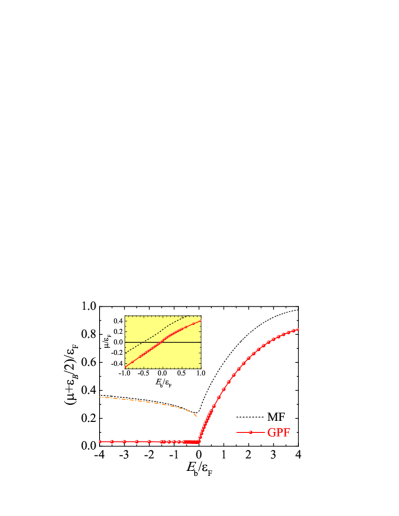
Figure 2: (color online). The chemical potential $\mu$ as a function of the scattering energy $E_{b}$, calculated by using the mean-field theory (dashed line) and GPF theory (solid line with circles). The dot-dashed line shows the asymptotic behavior in the BEC limit predicted by the mean-field theory in Eq. (50), which corresponds to a constant molecular scattering length for composite bosons. In the main figure, we have subtracted the contribution from the two-body bound state with the binding energy $\varepsilon_{B}\equiv\max(-E_{b},0)$. The inset highlights the chemical potential near the topological phase transition (i.e., $\mu\sim 0$ or $E_{b}\sim 0$). Here, we take a cut-off momentum $k_{0}=30k_{F}$.

In Fig. 2, we report the chemical potential $\mu$ as a function of the interaction strength $E_{b}$, predicted by the mean-field theory and GPF theory. To clearly show the many-body effect, we have subtracted the two-body contribution from the bound state when the scattering energy $E_{b}<0$, which takes the form $-\varepsilon_{B}/2\equiv-\max(-E_{b},0)/2$. In the BCS limit ($E_{b}\gg\varepsilon_{F}$), both mean-field and GPF theories predict $\mu\rightarrow\varepsilon_{F}$, as expected. However, towards the BEC limit ($E_{b}\ll-\varepsilon_{F}$), they show entirely different behavior.

In the BEC limit we anticipate that the system may turn into a weakly interacting Bose condensate of composite Cooper pairs, with a bosonic chemical potential given by,

$$\mu_{B}=2\mu+\varepsilon_{B}\simeq g_{B}n_{B},$$ (48)

where $n_{B}\simeq n/2$ and $g_{B}$ is the strength of the interaction between two Cooper pairs. Physically, $g_{B}$ should decrease as we move to the BEC limit. Using the relation $\varepsilon_{F}=2\pi\hbar^{2}n/m$, we obtain that

$$g_{B}\simeq\left(\frac{8\pi\hbar^{2}}{m}\right)\frac{\mu+\varepsilon_{B}/2}{\varepsilon_{F}}.$$ (49)

Thus, we observe from Fig. 2 that the mean-field theory incorrectly predicts an increasing pair-pair interaction strength when we approach the BEC limit, while the GPF theory gives a small residual pair-pair interaction, which is essentially independent on the scattering energy $E_{b}$.

In the mean-field theory, the pair-pair interaction strength can be analytically calculated using a Ginzburg-Landau free energy functional for the pair fluctuation field $\Delta_{\mathbf{q}}$ (see Appendix C). We find that,

$$g_{B,\textrm{MF}}=\frac{16\pi\hbar^{2}}{m}\frac{\left[\ln\eta+2\eta^{-1}-\eta^{-2}/2-3/2\right]}{\left(\ln\eta+\eta^{-1}-1\right)^{2}},$$ (50)

where $\eta=\hbar^{2}k_{0}^{2}/(m\left|E_{b}\right|)+1$. As $\eta\gg 1$ for the parameters in Fig. 2, to a good approximation we have

$$g_{B,\textrm{MF}}\simeq\frac{16\pi\hbar^{2}}{m}\frac{1}{\ln\left[\hbar^{2}k_{0}^{2}/\left(m\left|E_{b}\right|\right)\right]},$$ (51)

which explains the wrong behavior of stronger pair-pair interaction as we decrease $E_{b}$ (see the dot-dashed line in Fig. 2).

Quite generally, the mean-field theory breaks down in two dimensions due to enhanced quantum fluctuations. This is already known for an $s$-wave Fermi superfluid He2015 , where the mean-field theory predicts a constant pair-pair interaction strength of $4\pi\hbar^{2}/m$, instead of a much smaller and chemical potential dependent coupling strength. The renormalization of the pair-pair interaction due to quantum fluctuations is well-captured by our GPF theory. Indeed, in an $s$-wave Fermi superfluid the GPF theory is reliable in predicting an accurate molecular scattering length for composite bosons He2015 , in good agreement with the exact four-body calculation and diffusion quantum Monte Carlo (QMC) simulation. In our case of a chiral $p$-wave Fermi superfluid, we anticipate that the GPF theory will similarly lead to a reliable result for the pair-pair interaction strength $g_{B}$. Unfortunately, unlike the $s$-wave Fermi superfluid, the existence the regularization function $\Gamma\left({\bf k}\right)$ makes it infeasible to derive an analytic expression for $g_{B}$. In future studies, the QMC calculation of the ground-state energy of the system or the exact solution of four resonantly $p$-wave interacting fermions in two dimensions would be very useful to understand the small and constant pair-pair interaction strength $g_{B}$, as predicted by our GPF theory.

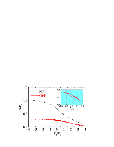
Figure 3: (color online). The pairing gap $\Delta$ as a function of the scattering energy $E_{b}$, predicted by using the mean-field theory (dashed line) and GPF theory (solid line with circles). The inset highlights the kink in the pairing gap near the topological phase transition (i.e., $E_{b}\sim 0$). Here, we take a cut-off momentum $k_{0}=30k_{F}$.

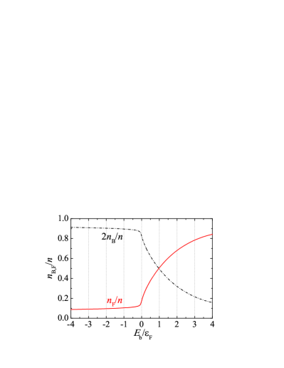
Figure 4: (color online). The fraction of fermions $n_{F}/n$ (solid line) and Cooper pairs $n_{B}/n$ (dashed line), as a function of the scattering energy $E_{b}$. Here, we take a cut-off momentum $k_{0}=30k_{F}$.

Let us now consider the intermediate coupling regime near zero scattering energy $E_{b}=0$, where the chemical potential $\mu$ changes sign and the system is expected to undergo a topological phase transition. In sharp contrast to the $s$-wave case, where $\mu$ evolves rather smoothly, here we find a dramatic change in the slope of the quantity $\mu+\varepsilon_{B}/2$ at $E_{b}\sim 0$ or $\mu\sim 0$. This non-analytic feature at the topological phase transition has been noticed in previous mean-field studies Botelho2005 ; Cao2013 ; Cao2017 and we see that quantum fluctuations make it even more pronounced.

Figure 3 presents the evolution of the pairing order parameter $\Delta$ as a function of the scattering energy $E_{b}$, calculated using the mean-field theory (dashed line) and the GPF theory (solid line with circles). Away from the BCS limit, the pairing gap is significantly reduced by quantum fluctuations. In particular, at resonance, the pairing gap is about a quarter of the Fermi energy, $\Delta\sim 0.25\varepsilon_{F}$. There is an apparent dip at the topological phase transition, as a result of the non-analyticity of the thermodynamics at the transition.

Theoretically, the significance of quantum fluctuations can be most easily recognized from the evolution of the number of Cooper pairs $n_{B}$ as a function of the scattering energy $E_{b}$, as shown in Fig. 4. We find a rapid increase in $n_{B}$, when we move to the topological phase transition point from the BCS limit. Upon reaching the transition, the dependence of the number of Cooper pairs on the scattering energy becomes nearly flat. Once again, this may be viewed as an indication of the non-analyticity at the topological phase transition.

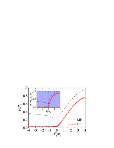
Figure 5: (color online). The pressure (main figure) and total energy (inset), as a function of the scattering energy $E_{b}$, predicted by using the mean-field theory (dashed line) and GPF theory (solid line with circles). The pressure and energy are normalized with respect to the ideal gas values $P_{0}=n\varepsilon_{F}/2$ and $E_{0}=N\varepsilon_{F}/2$, respectively. Here, $N$ is the total number of particles. For the total energy, we have subtracted the contribution from the two-body bound state, $-N\varepsilon_{B}/2$. As before, we take a cut-off momentum $k_{0}=30k_{F}$.

In experiments, on the other hand, the non-analyticity of the thermodynamic functions at the transition may be probed by measuring the homogeneous pressure equation of state through the density distribution of a harmonically trapped resonant $p$-wave Fermi superfluid Nascimbene2010 . In Fig. 5, we report the pressure $P$, normalized to its non-interacting value $P_{0}=n\varepsilon_{F}/2$, as a function of the scattering energy $E_{b}$, calculated with the mean-field theory and the GPF theory. The pressure $P$ shows almost the same scattering energy dependence as the chemical potential, with a clear kink at the topological phase transition. Therefore, the observation of this kink may be regarded as an indirect proof the topological phase transition TopoSuperfluidNote . Moreover, the measurement of the small and nearly constant pressure on the BEC side will be useful to clarify the nature of the resulting weak-interacting Bose condensate.

To conclude this subsection, it is worth noting a recent study of the same system by Jiang and Zhou Jiang2018 , based on a two-channel model for a broad $p$-wave resonance. In that study, quantum fluctuations from selected two-loop diagrams are found to destabilize the system at the resonance, in disagreement with our finding of a stable Fermi superfluid at all interaction strengths. This discrepancy is unlikely from the different model Hamiltonian (i.e., one-channel vs. two-channel), since the one-channel model and two-channel model are known to give the same description for a broad Feshbach resonance Diener2004 ; Liu2005 . It should come from the treatment of quantum fluctuations at different levels. The GPF treatment presented in this work, when it is generalized to the two-channel model Ohashi2003 , includes the two-loop diagrams selected by Jiang and Zhou Jiang2018 ; TwoLoopsDiagramNote . Moreover, it may pick up a set of marginal diagrams containing higher-order loops, within the ladder or bubble approximation. A future GPF study of the two-channel model for a resonantly interacting $p$-wave Fermi superfluid will be useful to clarify the discrepancy and to provide more accurate results for a narrow Feshbach resonance.

IV.2 Critical velocity for superfluidity

A superfluid loses its superfluidity when it moves faster than a critical velocity. For an $s$-wave Fermi superfluid, the critical velocity in the BCS and BEC limits is given by the pair-breaking velocity and sound velocity, respectively, and exhibits a maximum in between Diener2008 . A maximum critical velocity at the resonance emphasizes the stability of a strongly interacting Fermi superfluid Toniolo2017 .

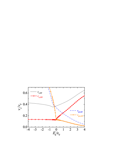
Figure 6: (color online). The sound velocity and pair-breaking velocity, as a function of the scattering energy $E_{b}$, predicted by using the mean-field theory (dashed line or dash-dotted line) and GPF theory (solid line with circles or stars). As the scattering energy decreases (or the interaction strength increases), the critical velocity $v_{c}=\max\{v_{pb},c_{s}\}$ slowly increases. Here, we take a cut-off momentum $k_{0}=30k_{F}$.

The situation for a $p$-wave Fermi superfluid seems to be a bit different. In Fig. 6, we present the sound velocity determined from the equation of state,

$$c_{s}=\left[\frac{n}{m}\frac{\partial\mu}{\partial n}\right]^{1/2}=\left[\frac{n}{m}\left(-\frac{\partial^{2}\Omega}{\partial\mu^{2}}\right)^{-1}\right]^{1/2},$$ (52)

and the pair-breaking velocity calculated by using Landau criterion,

$$v_{pb}=\min_{\{\mathbf{k}\}}\frac{E_{\mathbf{k}}}{\left|k\right|}\simeq\left\{\begin{array}[]{cc}\Delta&\textrm{if }\mu\geq 0\\ \sqrt{\Delta^{2}-4\mu}&\textrm{if }\mu<0\end{array}\right..$$ (53)

In both mean-field and GPF frameworks, the resulting critical velocity $v_{c}=\max\{v_{pb},c_{s}\}$ roughly increases with decreasing scattering energy $E_{b}$. In particular, on the BEC side, the GPF result of the critical velocity becomes nearly flat, consistent with a constant pair-pair interaction strength observed earlier. Typically, the critical velocity at resonance is about $0.1v_{F}$, smaller than that of an $s$-wave Fermi superfluid Bighin2016 ; Mulkerin2017 . This means that a $p$-wave Fermi superfluid could be more easily destroyed than its $s$-wave counterpart.

IV.3 BKT transition temperature

In two dimensions, the transition to a superfluid state at finite temperature is governed by the BKT mechanism Berezinskii1972 ; Kosterlitz1973 . The BKT critical temperature $T_{c}$ of a chiral $p$-wave Fermi superfluid was considered in the previous studies by using the mean-field theory Cao2017 . Here, we determine $T_{c}$ with the inclusion of quantum fluctuations.

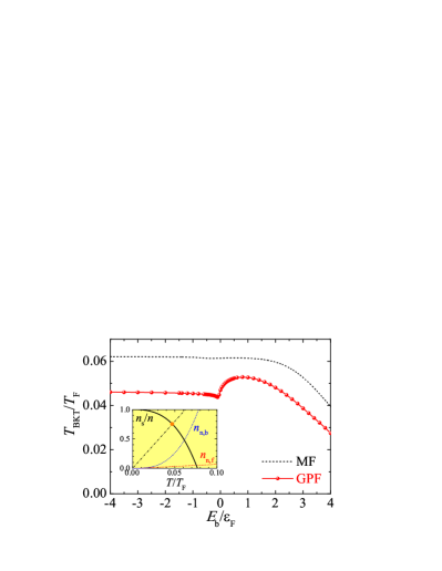
Figure 7: (color online). The BKT transition temperature, calculated by using the mean-field theory (dashed line) and GPF theory (solid line with circles), as a function of the scattering energy $E_{b}$. The inset shows the normal density fractions contributed by fermions $n_{n,f}/n$ and by pairs $n_{n,b}/n$, and the superfluid density fraction $n_{s}/n=1-n_{n,f}/n-n_{n,b}/n$ at zero scattering energy $E_{b}=0$. The cross point between the superfluid fraction $n_{s}/n$ and the line $16T/T_{F}$ determines the BKT temperature at $E_{b}=0$. Here, we take a cut-off momentum $k_{0}=30k_{F}$.

For this purpose, we need to calculate the superfluid density $n_{s}$ and then determine $T_{c}$ using the so-called Thouless-Nelson criterion Nelson1977 ,

$$k_{B}T_{c}=\frac{\pi\hbar^{2}}{8m}n_{s}\left(T_{c}\right),$$ (54)

or equivalently,

$$\frac{T_{c}}{T_{F}}=\frac{1}{16}\frac{n_{s}\left(T_{c}\right)}{n}.$$ (55)

A full calculation of superfluid density $n_{s}$ within the GPF framework is numerically involved. Here, we follow the idea by Bighin and Salasnich to approximately calculate the superfluid density using the standard Landau formalism Bighin2016 . This provides an approximate but convenient way to include quantum fluctuations Bighin2016 ; Mulkerin2017 .

To apply the Landau formalism, we assume that the low-energy excitations of the resonantly interacting $p$-wave superfluid are well-described by quasi-particles. This assumption is excellent in both BCS and BEC limits. Therefore, we anticipate that it may also give some qualitative predictions near resonance. Following Landau’s quasi-particle picture Khalatnikov2000 , the densities of the normal fluid, due to single-particle fermionic excitations and collective bosonic excitations, are respectively given by,

$$n_{n,f} = -\frac{\hbar^{2}}{m}\sum_{{\bf k}}\frac{{\bf k}^{2}}{2}\frac{\partial}{\partial E_{{\bf k}}}\left(\frac{1}{e^{E_{{\bf k}}/k_{B}T}+1}\right),$$ (56)

$$n_{n,b} = -\frac{\hbar^{2}}{m}\sum_{{\bf q}}\frac{{\bf q}^{2}}{2}\frac{\partial}{\partial\omega_{{\bf q}}}\left(\frac{1}{e^{\omega_{{\bf q}}/k_{B}T}-1}\right),$$ (57)

where we approximate that, as a rough estimation, the fermionic excitations have the energy spectrum of $E_{{\bf k}}$ and the bosonic excitations have phonon dispersion $\omega_{{\bf q}}\simeq c_{s}q$. The superfluid density $n_{s}$ then takes the form,

$$n_{s}=n-n_{n,f}-n_{n,b}.$$ (58)

At resonance, the normal densities due to fermionic and bosonic excitations, $n_{n,f}$ and $n_{n,b}$, and the superfluid density $n_{s}$ are shown in the inset of Fig. 7. We find that the bosonic degree of freedom gives the dominant contribution to the superfluid density and hence leads to a reduced BKT critical temperature. Indeed, the mean-field theory predicts a nearly saturated critical temperature $T_{c}=T_{F}/16\sim 0.06T_{F}$ at resonance, while our GPF theory with Landau formalism for superfluid density gives a smaller critical temperature $T_{c}\sim 0.04T_{F}$.

In the main figure of Fig. 7, we present the evolution of the BKT critical temperature $T_{c}$ as a function of the scattering energy $E_{b}$. It exhibits a bump near the resonance with a maximum $T_{c,\max}\simeq 0.052T_{F}$ at $E_{b}\sim\varepsilon_{F}$. The cusp at $E_{b}\simeq 0$ may be viewed as a clear demonstration of the non-analyticity of the finite temperature thermodynamics at the topological phase transition. Towards the BEC limit, we find that the BKT critical temperature saturates to $T_{c}\sim 0.047T_{F}$.

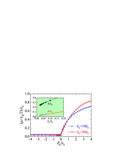
Figure 8: (color online). The chemical potential $\mu$ (with the two-body bound state contribution subtracted) as a function of the scattering energy $E_{b}$, at two cut-off momenta $k_{0}=10k_{F}$ (dashed line with stars) and $k_{0}=30k_{F}$ (solid line with circles). The inset shows the chemical potential $\mu$ and pairing gap $\Delta$ at the zero scattering energy $E_{b}=0$, as a function of the inverse cut-off momentum $k_{0}^{-1}$. All the results are predicted by using the GPF theory.

IV.4 The dependence on the cut-off momentum $k_{0}$

We now turn to discuss the cut-off momentum dependence of our results. In the main figure of Fig. 8, we compare the chemical potentials at the BEC-BCS evolution at two cut-off momenta, $k_{0}=10k_{F}$ (dashed line with stars) and $k_{0}=30k_{F}$ (solid line with circles). A factor of three reduction in the cut-off momentum does not lead to any changes at the qualitative level. In the inset, we highlight the cut-off momentum dependence of the chemical potential and pairing gap at the resonance. We do not find singular behaviors as we increase the cut-off momentum and extend it towards infinity. Therefore, although a cut-off momentum $k_{0}$ is necessary to make the $p$-wave interaction renormalizable (for dimensions $d\geq 2$), we may still have some universal behaviors that are weakly (i.e., logarithmically) dependent on $k_{0}^{-1}$.

V Conclusions and outlooks

In conclusions, we have theoretically investigated the consequence of quantum fluctuations in a resonantly interacting $p$-wave Fermi superfluid in two dimensions at the BEC-BCS evolution, using the Gaussian pair fluctuation theory. We have found that the zero-temperature equations of state, the critical velocity for superfluidity, and the BKT critical temperature are strongly renormalized by quantum fluctuations and their non-analyticity at the topological phase transition is greatly enhanced. Experimentally, this non-analyticity could be best probed by measuring the pressure equation of state at zero temperature, which shows an apparent kink near resonance, and the BKT critical temperature, which exhibits a bump and then a cusp structure. Although the $p$-wave Fermi superfluid seems to be delicate in superfluidity compared with its $s$-wave counterpart due to a smaller critical velocity, it is thermodynamically stable at all interaction strengths, in disagreement with a previous theoretical study Jiang2018 , which takes into account quantum fluctuations at the level of two-loop diagrams.

For $p$-wave interacting fermions in two dimensions, Nishida and co-workers recently predicted the existence of a series of three-particle bound states, the so-called super-Efimov states Nishida2013 . The impact of these super-Efimov states to the many-body properties (i.e., superfluidity) of the system remains to be understood. It will be an interesting research topic to be explored in future studies.

Appendix A Two-particle scattering

We use a separable interaction potential to characterize the chiral $p$-wave interatomic interaction:

$$V_{{\bf kk}^{\prime}} = \lambda\Gamma\left({\bf k}\right)\Gamma^{*}\left({\bf k}^{\prime}\right),$$ (59)

$$\Gamma\left({\bf k}\right) = \frac{\left(k/k_{1}\right)}{\left[1+\left(k/k_{0}\right)^{2n}\right]^{3/2}}e^{i\varphi_{{\bf k}}},$$ (60)

where $k_{1}$ - set to be $k_{F}$ in numerical calculations - is a characteristic momentum that makes $\Gamma\left({\bf k}\right)$ dimensionless, $k_{0}$ is a large-momentum cut-off, and $\varphi_{{\bf k}}$ is the polar angle of ${\bf k}$ in 2D momentum space. We use the exponent $n$ to control the shape of the regularization function $\Gamma\left({\bf k}\right)$. In the large-$n$ limit, effectively we have a step function.

To obtain the two-body scattering amplitude, we consider the following two-body $T$-matrix in vacuum,

$$T\left({\bf k},{\bf k}^{\prime};E_{+}\right) = t\left(E_{+}\right)\Gamma\left({\bf k}\right)\Gamma^{*}\left({\bf k}^{\prime}\right),$$ (61)

$$\frac{1}{t\left(E_{+}\right)} = \frac{1}{\lambda}+\sum_{{\bf k}^{\prime\prime}}\frac{\left|\Gamma\left({\bf k}^{\prime\prime}\right)\right|^{2}}{2\epsilon_{{\bf k}^{\prime\prime}}-E_{+}},$$ (62)

where $k^{\prime}=\left|{\bf k}^{\prime}\right|=k$ and $E_{+}=\hbar^{2}k^{2}/m+i0^{+}$. The analytic form of the scattering amplitude or $t\left(E_{+}\right)$ in the low energy limit (i.e., $k\rightarrow 0$) should be independent on the detailed regularization function. Therefore, we may simply use a step function (i.e., $n\rightarrow\infty$). By introducing a new variable $x=(k^{\prime\prime})^{2}$, we find that,

$$\frac{1}{t\left(E_{+}\right)}=\frac{1}{\lambda}+\frac{m}{4\pi\hbar^{2}k_{1}^{2}}\int\limits_{0}^{k_{0}^{2}}dx\frac{x}{x-\tilde{E}_{+}},$$ (63)

where $\tilde{E}_{+}=k^{2}+i0^{+}$. This leads to ($\tilde{E}=k^{2}$),

$$\frac{1}{t\left(E_{+}\right)}=\frac{1}{\lambda}+\frac{m}{4\pi\hbar^{2}k_{1}^{2}}\left[k_{0}^{2}+\tilde{E}\ln\left(\frac{k_{0}^{2}}{\tilde{E}}-1\right)+i\pi\tilde{E}\right].$$ (64)

By taking the low-energy limit $k\rightarrow 0$, we arrive at

$$\frac{1}{t\left(E_{+}\right)}=-\frac{m}{4\hbar^{2}k_{1}^{2}}\left[-\frac{1}{a_{p}}+\frac{2k^{2}}{\pi}\ln\left(R_{p}k\right)-ik^{2}\right],$$ (65)

where $R_{p}\sim 1/k_{0}$ is the effective range of the $p$-wave interaction, the term $a_{p}^{-1}$ collects all the constants in Eq. (64) and physically we interpret $a_{p}$ as the $p$-wave scattering area in two dimensions. It is easy to see that, the full two-body $T$-matrix is ($k=k^{\prime}$),

$$T\left({\bf k},{\bf k}^{\prime};E_{+}\right)=e^{i\left(\varphi_{{\bf k}}-\varphi_{{\bf k}^{\prime}}\right)}\left(-\frac{4\hbar^{2}}{m}\right)\left[\frac{kk^{\prime}}{-a_{p}^{-1}+\left(2k^{2}/\pi\right)\ln\left(R_{p}k\right)-ik^{2}}\right].$$ (66)

According to Levinsen, Cooper and Gurarie (see Appendix in Ref.Levinsen2008 ), we may define a two-dimensional $p$-wave scattering amplitude,

$$f_{p}\left(k\right)=-\frac{m}{2\hbar^{2}\left(2\pi k\right)^{1/2}}T\left({\bf k},{\bf k};E_{+}\right)=\sqrt{\frac{2}{\pi k}}\frac{k^{2}}{-a_{p}^{-1}+\left(2k^{2}/\pi\right)\ln\left(R_{p}k\right)-ik^{2}}=\frac{1}{g_{p}(k)-i\left(\pi k/2\right)^{1/2}},$$ (67)

where

$$g_{p}(k)=\sqrt{\frac{\pi k}{2}}\frac{-a_{p}^{-1}+\left(2k^{2}/\pi\right)\ln\left(R_{p}k\right)}{k^{2}}$$ (68)

is a real function of $k$. The $p$-wave scattering amplitude may also be written in terms of the phase shift $\delta_{p}(k)$ Levinsen2008 :

$$f_{p}\left(k\right)=\frac{1}{i\sqrt{2\pi k}}\left(e^{2i\delta_{p}}-1\right)=\sqrt{\frac{2}{\pi k}}\frac{1}{\cot\delta_{p}-i},$$ (69)

where the phase shift satisfies,

$$k^{2}\cot\delta_{p}\left(k\right)=-\frac{1}{a_{p}}+\frac{2k^{2}}{\pi}\ln\left(R_{p}k\right)+\cdots.$$ (70)

We note that, the relation between the scattering amplitude $f_{p}(k)$ and phase shift $\delta_{p}(k)$ defined in Eq. (69) is slightly different from that derived by solving the two-body problem (see Eq. (11) in Ref. Zhang2017 )

Appendix B The structure of the functions $A$, $B$, $C$, $D$ and $F$

Here we demonstrate that the functions $A$, $B$, $C$, $D$ and $F$ do not depend on the direction of ${\bf q}$, and thus we may simply set ${\bf q}=q{\bf e}_{x}$ in numerical calculations. Actually, this is pretty clear for $A$, $B$, $C$ and $D$, since the factor $\left|\Gamma({\bf k)}\right|$ does not depend on the polar angle $\varphi_{{\bf k}}$. All the integral functions therefore depend on the angle between ${\bf q}$ and ${\bf k}$ only, or more precisely $\cos(\varphi_{{\bf k}}-\varphi_{{\bf q}})$. For the function $F$, we now need to check explicitly that the factor

$$P=\Gamma^{*}\left({\bf k}\right)\Gamma^{*}\left({\bf k}\right)\Gamma\left(\frac{\mathbf{q}}{2}+{\bf k}\right)\Gamma\left(\frac{\mathbf{q}}{2}-{\bf k}\right)$$ (71)

also depends on $\varphi_{{\bf k}}-\varphi_{{\bf q}}$ only. We may also explicitly show that $F$ is a real function. For this purpose, we examine the following product,

$$P = \tilde{P}\left(k,q;\varphi_{{\bf k}}-\varphi_{{\bf q}}\right)e^{-i2\varphi_{{\bf k}}}\left[\left(\frac{q_{x}}{2}+k_{x}\right)+i\left(\frac{q_{y}}{2}+k_{y}\right)\right]\left[\left(\frac{q_{x}}{2}-k_{x}\right)+i\left(\frac{q_{y}}{2}-k_{y}\right)\right],$$ (72)

$$= \tilde{P}\left(k,q;\varphi_{{\bf k}}-\varphi_{{\bf q}}\right)e^{-i2\varphi_{{\bf k}}}\left[\frac{\left(q_{x}^{2}-q_{y}^{2}\right)}{4}-\left(k_{x}^{2}-k_{y}^{2}\right)+i2\left(\frac{q_{x}q_{y}}{4}-k_{x}k_{y}\right)\right],$$ (73)

$$= \tilde{P}\left(k,q;\varphi_{{\bf k}}-\varphi_{{\bf q}}\right)\left[\cos 2\varphi_{{\bf k}}-i\sin 2\varphi_{{\bf k}}\right]\left[\left(\frac{q^{2}}{4}\cos 2\varphi_{{\bf q}}-k^{2}\cos 2\varphi_{{\bf k}}\right)+i\left(\frac{q^{2}}{4}\sin 2\varphi_{{\bf q}}-k^{2}\sin 2\varphi_{{\bf k}}\right)\right]$$ (74)

$$= \tilde{P}\left(k,q;\varphi_{{\bf k}}-\varphi_{{\bf q}}\right)\left\{\left[\frac{q^{2}}{4}\cos\left(2\varphi_{{\bf k}}-2\varphi_{{\bf q}}\right)-k^{2}\right]-i\frac{q^{2}}{4}\sin\left(2\varphi_{{\bf k}}-2\varphi_{{\bf q}}\right)\right\},$$ (75)

where in the first line of the equation, we have singled out the chiral $p_{x}+ip_{y}$ dependence of the regularization function $\Gamma$ and the function $\tilde{P}$ depends on $\varphi_{{\bf k}}-\varphi_{{\bf q}}$. It is now clear that, in the calculations of $A$, $B$, $C$, $D$ and $F$, $\varphi_{{\bf q}}$ can be removed by re-defining the angle $\varphi_{{\bf k}}$: $\varphi_{{\bf k}}-\varphi_{{\bf q}}\rightarrow\varphi$. The imaginary part of $F$ is strictly zero since

$$\int\limits_{0}^{2\pi}d\varphi h\left(\cos\varphi\right)\sin 2\varphi=0$$ (76)

for any function $h(x)$.

Appendix C Ginzburg-Landau free energy functional for the pair fluctuation field

In the BEC limit, we may derive a Gross-Pitaevskii free energy of composite bosons $\mathcal{S}[\phi(\mathbf{x},\tau)]$, which takes the form,

$$\mathcal{S}=\int dx\left[\phi^{*}\left(\frac{\partial}{\partial\tau}-\frac{\hbar^{2}}{2m_{B}}-\mu_{B}\right)\phi+\frac{g_{B}}{2}\left|\phi\right|^{4}\right],$$ (77)

where $m_{B}=2m$ is the mass of composite bosons, $\mu_{B}$ is the chemical potential and $g_{B}$ is the pair-pair interaction strength, and we abbreviate $x\equiv(\mathbf{x},\tau)$. To this end, we first consider the Ginzburg-Landau free energy functional for the pair fluctuation field $\Delta(x)$:

$$\mathcal{\tilde{S}}=\int dx\left[\Delta^{*}\left(a\frac{\partial}{\partial\tau}-b\frac{\hbar^{2}}{4m}-c\right)\Delta+\frac{d}{2}\left|\Delta\right|^{4}\right],$$ (78)

where the $\phi$-field can be obtained by rescaling the pair fluctuation field $\Delta$, i.e., $\sqrt{a}\Delta(x)\rightarrow\phi(x)$.

Following the seminal work by Sá de Melo, Randeria, and Engelbrecht SadeMelo1993 , we determine the coefficients $a$, $b$, and $c$ by evaluating the small frequency and momentum expansion of the pair propagator $M_{0}(\mathbf{q},i\nu_{n})$ in the normal state, which takes the form,

$$M_{0}=-\frac{1}{2\lambda}+\frac{1}{2}\sum_{\mathbf{k}}\frac{\left|\Gamma(\mathbf{k})\right|^{2}}{i\nu_{n}+2\mu-2\epsilon_{\mathbf{k}}-\hbar^{2}\mathbf{q}^{2}/(4m)}.$$ (79)

Using the fact that,

$$M_{0}\left(\mathbf{q}\rightarrow 0,i\nu_{n}\rightarrow 0\right)\simeq-a\left(i\nu_{n}\right)+b\frac{\hbar^{2}\mathbf{q}^{2}}{4m}-c,$$ (80)

we obtain

$$a=b=\frac{1}{2}\sum_{\mathbf{k}}\frac{\left|\Gamma(\mathbf{k})\right|^{2}}{\left(2\epsilon_{\mathbf{k}}-2\mu\right)^{2}}$$ (81)

and

$$c=\frac{1}{2\lambda}+\frac{1}{2}\sum_{\mathbf{k}}\frac{\left|\Gamma(\mathbf{k})\right|^{2}}{2\epsilon_{\mathbf{k}}-2\mu}.$$ (82)

In the BEC limit, we have $\mu_{B}=2\mu-E_{b}\rightarrow 0^{+}$. By replacing the bare interaction strength $\lambda$ with the scattering energy $E_{b}$, it is easy to verify that,

$$c\simeq\frac{\mu_{B}}{2}\sum_{\mathbf{k}}\frac{\left|\Gamma(\mathbf{k})\right|^{2}}{\left(2\epsilon_{\mathbf{k}}+\left|E_{b}\right|\right)^{2}}\simeq\mu_{B}a.$$ (83)

The integral in $a$ can be worked out in the limit of an infinitely large exponent $n\rightarrow\infty$, where $\Gamma(\mathbf{k})=[(k_{x}+ik_{y})/k_{1}]\Theta(k_{0}-k)$. We find that,

$$a=\frac{m^{2}}{8\pi\hbar^{4}k_{1}^{2}}\left(\ln\eta+\frac{1}{\eta}-1\right),$$ (84)

where $\eta=\hbar^{2}k_{0}^{2}/(m\left|E_{b}\right|)+1$.

The coefficient $d$, on the other hand, may be calculated by Taylor expanding the mean-field thermodynamic potential $\Omega_{\textrm{MF}}$ at small pairing gap $\Delta\sim 0$, i.e.,

$$\Omega_{\textrm{MF}} = -c\Delta^{2}+\frac{d}{2}\Delta^{4}+\cdots.$$

This leads to,

$$c=-\frac{\partial\Omega_{\textrm{MF}}}{\partial\Delta^{2}}=\frac{1}{2\lambda}+\sum_{\mathbf{k}}\frac{\left|\Gamma(\mathbf{k})\right|^{2}}{2\epsilon_{\mathbf{k}}-2\mu}$$ (85)

as anticipated, and

$$d=\frac{\partial^{2}\Omega_{\textrm{MF}}}{\partial\left(\Delta^{2}\right)^{2}}=\sum_{\mathbf{k}}\frac{\left|\Gamma(\mathbf{k})\right|^{4}}{\left(2\epsilon_{\mathbf{k}}-2\mu\right)^{3}}.$$ (86)

By replacing $-2\mu$ with $\left|E_{b}\right|$ in the equation for $d$, and performing the integration, we obtain,

$$d = \frac{m^{3}}{4\pi\hbar^{6}k_{1}^{4}}\left(\ln\eta+\frac{2}{\eta}-\frac{1}{2\eta^{2}}-\frac{3}{2}\right).$$ (87)

The rescaling of the pair fluctuation field, $\sqrt{a}\Delta(x)\rightarrow\phi(x)$, leads to the desired expression for the pair-pair interaction strength,

$$g_{B}=\frac{d}{a^{2}}=\frac{16\pi\hbar^{2}}{m}\frac{\left[\ln\eta+2\eta^{-1}-\eta^{-2}/2-3/2\right]}{\left(\ln\eta+\eta^{-1}-1\right)^{2}},$$ (88)

which is Eq. (50) in the main text.

References

• (1) V. P. Mineev and K. V. Samokhin, Introduction to Unconventional Superconductivity (CRC, Boca Raton, FL, 1999).
• (2) N. Read and D. Green, Phys. Rev. B 61, 10267 (2000).
• (3) D. A. Ivanov, Phys. Rev. Lett. 86, 268 (2001).
• (4) A. Yu. Kitaev, Ann. Phys. (NY) 303, 2 (2003).
• (5) For a review, see, C. Nayak, S. H. Simon, A. Stern, M. Freedman, and S. D. Sarma, Rev. Mod. Phys. 80, 1083 (2008).
• (6) Y. Maeno, H. Hashimoto, K. Yoshida, S. Nishizaki, T. Fujita, J. G. Bednorz, and F. Lichtenberg, Nature (London) 372, 532 (1994).
• (7) For a review, see, V. Gurarie and L. Radzihovsky, Ann. Phys. (Amsterdam) 322, 2 (2007).
• (8) I. Bloch, J. Dalibard, and W. Zwerger, Rev. Mod. Phys. 80, 885 (2008).
• (9) S. Giorgini, L. P. Pitaevskii, and S. Stringari, Rev. Mod. Phys. 80, 1215 (2008).
• (10) D. M. Eagles, Phys. Rev. 186, 456 (1969).
• (11) A. J. Leggett, in Modern Trends in the Theory of Condensed Matter, edited by A. Pekalski and R. Przystaw (Springer-Verlag, Berlin, 1980).
• (12) P. Noziéres and S. Schmitt-Rink, J. Low Temp. Phys. 59, 195 (1985).
• (13) C. A. R. Sá de Melo, M. Randeria, and J. R. Engelbrecht, Phys. Rev. Lett. 71, 3202 (1993).
• (14) C. A. Regal, C. Ticknor, J. L. Bohn, and D. S. Jin, Phys. Rev. Lett. 90, 053201 (2003).
• (15) J. Zhang, E. G. M. van Kempen, T. Bourdel, L. Khaykovich, J. Cubizolles, F. Chevy, M. Teichmann, L. Tarruell, S. J. J. M. F. Kokkelmans, and C. Salomon, Phys. Rev. A 70, 030702(R) (2004).
• (16) K. Günter, T. Stöferle, H. Moritz, M. Köhl, and T. Esslinger, Phys. Rev. Lett. 95, 230401 (2005).
• (17) C. H. Schunck, M. W. Zwierlein, C. A. Stan, S. M. F. Raupach, W. Ketterle, A. Simoni, E. Tiesinga, C. J. Williams, and P. S. Julienne, Phys. Rev. A 71, 045601 (2005).
• (18) J. P. Gaebler, J. T. Stewart, J. L. Bohn, and D. S. Jin, Phys. Rev. Lett. 98, 200403 (2007).
• (19) J. Fuchs, C. Ticknor, P. Dyke, G. Veeravalli, E. Kuhnle, W. Rowlands, P. Hannaford, and C. J.Vale, Phys. Rev.A 77, 053616 (2008).
• (20) Y. Inada, M. Horikoshi, S. Nakajima, M. Kuwata-Gonokami, M. Ueda, and T. Mukaiyama, Phys. Rev. Lett. 101, 100401 (2008).
• (21) T. Nakasuji, J. Yoshida, and T. Mukaiyama, Phys. Rev. A 88, 012710 (2013).
• (22) C. Luciuk, S. Trotzky, S. Smale, Z. Yu, S. Zhang, and J. H. Thywissen, Nat. Phys. 12, 599 (2016).
• (23) M. Waseem, T. Saito, J. Yoshida, and T. Mukaiyama, Phys. Rev. A 96, 062704 (2017).
• (24) J. Yoshida, T. Saito, M. Waseem, K. Hattori, and T. Mukaiyama, Phys. Rev. Lett. 120, 133401 (2018).
• (25) M. Waseem, J. Yoshida, T. Saito, and T. Mukaiyama, Phys. Rev. A 98, 020702(R) (2018).
• (26) J. Levinsen, N. R. Cooper, and V. Gurarie, Phys. Rev. A, 78, 063616 (2008).
• (27) A. K. Fedorov, V. I. Yudson, and G. V. Shlyapnikov, Phys. Rev. A 95, 043615 (2017).
• (28) M. Lu, N. Q. Burdick, and B. L. Lev, Phys. Rev. Lett. 108, 215301 (2012).
• (29) K. Aikawa, S. Baier, A. Frisch, M. Mark, C. Ravensbergen, and F. Ferlaino, Science 345, 1484 (2014).
• (30) S. S. Botelho and C. A. R. Sa de Melo, J. Low Temp. Phys. 140, 409 (2005).
• (31) T.-L. Ho and R. B. Diener, Phys. Rev. Lett. 94, 090402 (2005).
• (32) V. Gurarie, L. Radzihovsky, and A. V. Andreev, Phys. Rev. Lett. 94, 230403 (2005).
• (33) C.-H. Cheng and S.-K. Yip, Phys. Rev. Lett. 95, 070404 (2005).
• (34) M. Iskin and C. A. R. Sá de Melo, Phys. Rev. Lett. 96, 040402 (2006).
• (35) G. Cao, L. He, and P. Zhuang, Phys. Rev. A 87, 013613 (2013).
• (36) Y. Ohashi, Phys. Rev. Lett. 94, 050403 (2005).
• (37) D. Inotani, R. Watanabe, M. Sigrist, and Y. Ohashi, Phys. Rev. A 85, 053628 (2012).
• (38) D. Inotani and Y. Ohashi, Phys. Rev. A 92, 063638 (2015).
• (39) G. Cao, L. He, and X.-G. Huang, Phys. Rev. A 96, 063618 (2017).
• (40) S. M. Yoshida and M. Ueda, Phys.Rev. Lett. 115, 135303 (2015).
• (41) Z. Yu, J. H. Thywissen, and S. Zhang, Phys. Rev. Lett. 115, 135304 (2015).
• (42) M. He, S. Zhang, H. M. Chan, and Q. Zhou, Phys. Rev. Lett. 116, 045301 (2016).
• (43) S.-G. Peng, X.-J. Liu, and H. Hu, Phys. Rev. A 94, 063651 (2016).
• (44) Y.-C. Zhang and S. Zhang, Phys. Rev. A 95, 023603 (2017).
• (45) J. Yao and S. Zhang, Phys. Rev. A 97, 043612 (2018).
• (46) D. Inotani and Y. Ohashi, Phys. Rev. A 98, 023603 (2018).
• (47) S. Tan, Ann. Phys. (NY) 323, 2952 (2008).
• (48) E. Braaten and L. Platter, Phys. Rev. Lett. 100, 205301 (2008).
• (49) G. Liu and Y.-C. Zhang, Europhys. Lett. 122, 40006 (2018).
• (50) S.-J. Jiang and F. Zhou, Phys. Rev. A 97, 063606 (2018).
• (51) H. Hu, X.-J. Liu, and P. D. Drummond, Europhys. Lett. 74, 574 (2006).
• (52) R. B. Diener, R. Sensarma, and M. Randeria, Phys. Rev. A 77, 023626 (2008).
• (53) H. Hu, P. D. Drummond, and X.-J. Liu, Nat. Phys. 3, 469 (2007).
• (54) L. He, H. Lü, G. Cao, H. Hu, and X.-J. Liu, Phys. Rev. A 92, 023620 (2015).
• (55) G. Bighin and L. Salasnich, Phys. Rev. B 93, 014519 (2016).
• (56) A. A. Abrikosov, L. Gor’kov, and I. E. Dzyaloshinski, Methods of Quantum Field Theory in Statistical Physics (Dover, New York, 1963).
• (57) S. Nascimbène, N. Navon, K. Jiang, F. Chevy, and C. Salomon, Nature (London) 463, 1057 (2010).
• (58) In order to have a smoking gun proof of the non-trivial topological properties of the Fermi superfluid, it is necessary to confirm the existence of the chiral Majorana mode at the edge or the non-abelian Majorana fermions at the vortex core.
• (59) R. B. Diener and T.-L. Ho, arXiv:cond-mat/0405174 (2004).
• (60) X.-J. Liu and H. Hu, Phys. Rev. A 72, 063613 (2005).
• (61) Y. Ohashi and A. Griffin Phys. Rev. A 67, 063612 (2003).
• (62) In our numerical GPF calculations, we avoid some approximations made by Jiang and Zhou to the two-loop diagrams for obtaining a closed analytic form for the thermodynamic potential Jiang2018 .
• (63) U. Toniolo, B. C. Mulkerin, C. J. Vale, X.-J. Liu, and H. Hu, Phys. Rev. A 96, 041604(R) (2017).
• (64) V. L. Berezinskii, Zh. Eksp. Teor. Fiz. 61, 1144 (1971) [Sov. Phys. JETP 34, 610 (1972)].
• (65) J. M. Kosterlitz and D. J. Thouless, J. Phys. C 6, 1181 (1973).
• (66) D. R. Nelson and J. M. Kosterlitz, Phys. Rev. Lett. 39, 1201 (1977).
• (67) B. C. Mulkerin, L. He, P. Dyke, C. J. Vale, X.-J. Liu, and H. Hu, Phys. Rev. A 96, 053608 (2017).
• (68) I. M. Khalatnikov, An Introduction to the Theory of Superfluidity (The Perseus Books Group, Boulder, 2000).
• (69) Y. Nishida, S. Moroz, and D. T. Son, Phys. Rev. Lett. 110, 235301 (2013).