Preparing multiparticle entangled states of NV centers via adiabatic ground-state transitions
Abstract
We propose an efficient method to generate multiparticle entangled states of NV centers in a spin mechanical system, where the spins interact through a collective coupling of the Lipkin-Meshkov-Glick (LMG) type. We show that, through adiabatic transitions in the ground state of the LMG Hamiltonian, the Greenberger-Horne-Zeilinger (GHZ)-type or the W-type entangled states of the NV spins can be generated with this hybrid system from an initial product state. Because of adiabaticity, this scheme is robust against practical noise and experimental imperfection, and may be useful for quantum information processing.
I introduction
In recent years, much attention has been paid to the generation of multiparticle entangled states with different systems, which play a key role in quantum computation, quantum networks, quantum teleportation, and quantum cryptography Wootters (1998); Vedral (2002); Horodecki et al. (2009); Sørensen and Mølmer (1999); James (1998); Raussendorf and Briegel (2001); Dakić and Radonjić (2017). Thus far, a plenty of schemes for preparing multiparticle entangled states have been proposed, with a variety of setups such as ion traps, cavity QED, spin-mechanics, etc Cirac and Zoller (1995); Zheng (2001); Mølmer and Sørensen (1999); Unanyan et al. (2001); Unanyan and Fleischhauer (2003); Morrison and Parkins (2008); Møller et al. (2008); Zhang and Duan (2013); Reiter et al. (2016); Armata et al. (2017); Ashhab et al. (2008); Li et al. (2017); Yang et al. (2012, 2013). Furthermore, some of these schemes have been successfully implemented in experiment Häffner et al. (2005); Meekhof et al. (1996); Barontini et al. (2015); Neumann et al. (2008); Sackett et al. (2000); Zhu et al. (2011); Johnson et al. (2017). Especially, hybrid quantum systems are reliable and promising setups for quantum information processing due to their easy scalability and longer coherence times Xiang et al. (2013a); Rabl et al. (2006); Peng et al. (2012); Xiang et al. (2013b); Lü et al. (2013); Song et al. (2017); Houck et al. (2016); Buluta et al. (2012); You and Nori (2005).
Among all microscopic solid state systems, nitrogen-vacancy (NV) centers in diamond are particularly attractive due to their excellent spin properties even at ambient conditions Hong et al. (2012); Doherty et al. (2013); Maze et al. (2011); Kubo et al. (2010, 2011); MacQuarrie et al. (2013); Golter et al. (2016a); Teissier et al. (2014); Bar-Gill et al. (2013); Maze et al. (2011); Doherty et al. (2012). Significant theoretical and experimental investigations have been carried out to realize quantum logical gates, quantum state manipulating, and entangled state generation Golter and Wang (2014); Golter et al. (2014, 2016b). However, it is still a challenge to generate multipartite entanglement among distant NV centers in hybrid quantum systems Dai and Kwek (2012); Sipahigil et al. (2012); Yang et al. (2011); Xia and Twamley (2016).
In principle, the precondition for manipulating or entangling NV spins is to acquire the strong coupling between the NV spins and other quantum data buses Li et al. (2016); Bennett et al. (2013); Li and Nori (2018); Amsüss et al. (2011); You et al. (2014). Much work has been proposed by taking advantage of the strong magnetic coupling between NV center ensembles and superconducting microwave cavities or qubits Kubo et al. (2010, 2011); Marcos et al. (2010); Zou et al. (2014); Zhou et al. (2017). In fact, the more attractive investigation is the strong magnetic coupling between nanomechanical resonators (NAMR) and single NV centers or a few of distant NV centers Dolde et al. (2011); Albrecht et al. (2013); Rabl et al. (2009); Xu et al. (2009); Ma et al. (2017). Based on the spin-mechanical system, several promising theoretical schemes have also been proposed to prepare entangled NV spins by utilizing the NAMR as a data bus Li et al. (2016); Xia and Twamley (2016); Xu et al. (2009); Ma et al. (2017); Rabl et al. (2010). Since these schemes naturally rely on the dynamical evolution of the hybrid spin mechanical system, the target state is inevitably disturbed by dissipations and ambient thermal noises. Therefore, it is appealing to propose a high-efficiency and more feasible protocol for preparing multiparticle entangled NV spins.
In this work, we propose an efficient scheme for generating multiparticle entangled states of NV centers in a spin mechanical system, where an array of NV centers are magnetically coupled to a nanomechanical resonator. With the assistance of external microwave fields, we can acquire collective interactions for NV spins with the form of the Lipkin-Meshkov-Glick (LMG) type Lipkin et al. (1965) The LMG Hamiltonian can be adiabatically steered from the isotropic type to the one-axis twisting one by tuning the Rabi frequencies slowly enough to maintain the NV spins in the ground state. The collective NV spins undergo the ground-state transitions that allows us to obtain the adiabatic channels between the initial separate ground state and the final entangled ground state. We investigate this adiabatic scheme with analytical results and numerical simulations for three different types of adiabatic transfer processes. The results indicate that we can acquire the Greenberger-Horne-Zeilinger (GHZ)-type and the W-type entangled states for NV spins with very high fidelity. Compared to previous works, this scheme is robust against practical noise and experimental imperfection because of adiabaticity.
II The setup

We consider the spin-mechanical setups as illustrated in Fig. 1(a) and (b). The ground-state energy level structure of a single NV center is shown in Fig. 1(c). The electronic ground triplet state is the eigenstates of spin operator with , and the zero-field splitting between the degenerate sublevels and is GHz Doherty et al. (2012); Maze et al. (2011); Doherty et al. (2013). A homogeneous static magnetic field is used to remove the degenerate states with the Zeeman splitting . In Fig. 1(a), the end of a cantilever NAMR with dimensions is attached with a row of equidistant magnet tips (size of nm). An array of NV centers are placed homogeneously and sparsely in the vicinity of the upper surface of the diamond sample, which are placed just under the magnet tips one-by-one with the same distance nm. The motion of the cantilever attached with the magnet chip produces the time-dependent gradient magnetic field , with the fundamental frequency at the NV spinDolde et al. (2011); Albrecht et al. (2013); Rabl et al. (2009); Xu et al. (2009); Ma et al. (2017). Meanwhile, we apply the dichromatic microwave driving fields polarized in the direction with frequencies and to manipulate the NV centers’ triple ground states. To make sure that the NV centers are all strongly and nearly equally coupled to the cantilever, we restrict the tips within a small region near the end of the cantilever. In this case, the number for available NV centers is limited to at most 10 NV centers Rabl et al. (2009); Xu et al. (2009). Moreover, we assume that the dichromatic microwave fields drive the NV centers homogeneously, because the microwave length is much larger than the size of the the cantilever.
Then for the single NV spin, we can obtain the Hamiltonian expressed as
| (1) | |||||
where is the landé factor of NV center, is the Bohr magneton, and is the spin operator of the NV center. As , we can ignore the far-off resonant interactions between the spin and the gradient magnetic fields along and directions. Then we can obtain the Hamiltonian
| (2) | |||||
We assume , with the first order gradient magnetic field, and the corresponding annihilation and creation operators, and the zero field fluctuation for this resonator of mass . In the rotating frame at the frequency ,
| (3) | |||||
where is the coupling constant between the NV center and the NAMR. Taking and , we assume the frequencies of the two driving fields and are far off resonance with respect to the transition between the states and . Therefore, this allows us to isolate a two-level subsystem comprised by for the single NV center. For the NV spin, we can define , , and . Then we can obtain the Hamiltonian under the rotating-wave approximation,
| (4) | |||||
where is the energy transition frequency between the level and , and are the dichromatic Rabi frequencies.
We can ignore the interactions between the adjacent NV centers, as long as the distance between the two adjacent NV spins is far enough. Then we have the total Hamiltonian for this hybrid system
| (5) | |||||
The first and second items are the free Hamiltonian for the NAMR and NV centers, the third item is the Hamiltonian for describing the interactions between the NV centers and the mechanical resonator, and the last item describes the microwave driving for the transition between and of the NV spins.
We can also implement such a spin-mechanical setup by use of a suspended carbon nanotube resonator that carries dc current. Recently, it has been shown that the suspended carbon nanotube carrying dc current can enable the strong coupling between mechanical motion and NV spins Li et al. (2016). This setup is particularly suitable for the investigation of an array of NV centers coupled to a mechanical resonator.
Another equivalent setup is illustrated in Fig. 1(b). In this system, a row of equidistant NV centers are set homogeneously and sparsely in the vicinity of the upper surface near the end of the cantilever diamond NAMR. An array of magnetic tips are fixed above these NV centers one-by-one with the same distance . With the assistance of the static magnetic fields and microwave driving fields, we can also achieve the equivalent Hamiltonian for describing the interactions as the first setup shown in Fig. 1(a).
Owing to the variations in the size and spacing of the nanomagnets and NV centers, the coupling can not be the same for all of the NV centers. There will be slight differences for each NV center, and this will give rise to a degree of disorder in the system. Here we define and , where is the disorder factor in this hybrid system Janarek et al. (2018); Underwood et al. (2012); Ashhab (2015); de Abreu et al. (2018). Therefore, the Hamiltonian in Eq. (5) can be expressed as
| (6) | |||||
For conveniently, we define the collective spin operators for all of the NV centers as , , , and they also satisfy the angular momentum commutation relations . Therefore, Eq. (6) can be simplified as
| (7) | |||||
First of all, we apply the unitary Schrieffer-Wolff transformation to , where , and can be viewed as an effective Lamb-Dicke parameter for this solid-state system Albrecht et al. (2013); Golter et al. (2016b); Rabl et al. (2010). Then we have .
| (8) | |||||
where is the coefficient of Ising interactions. and are the experimental disorder items in our system. The first item corresponds to the high frequency oscillating item, and its effective influence on the system can be discarded because . The second item corresponds to the major disorder, whose effect will be discussed in Sec. V. For simplicity, we first assume that , and then we can discard the item because of . As a result, we can acquire the Hamiltonian without the disorder
| (9) | |||||
Secondly, we assume that the resonator is cooled sufficiently with extremely low ambient temperature, so that this hybrid system satisfies the Lamb-Dicke limit , where is the average number of the phonon for this oscillation mode with temperature Cirac and Zoller (1995); Mølmer and Sørensen (1999); Zheng (2001); Unanyan et al. (2001); Unanyan and Fleischhauer (2003). Applying the approximate relation to Eq. (9) we can acquire the Hamiltonian in the interaction picture
| (10) |
We define the detuning as , and assume the relations in this hybrid system , , and . Since the NAMR stays in relative lower energy state, we can eliminate the resonator mode and ignore the items for the energy shift caused by this mechanical oscillation mode. Then we can get the effective Hamiltonian as follow James and Jerke (2012)
| (11) |
where the effective coefficients are
| (12) |
According to Eq. (11), the effective Hamiltonian for this system evidently corresponds to the general LMG model for describing the collective interactions of spin- particles.
Therefore, in this solid-state system, we introduce the single NV center’s decoherence factor as the dephasing rate to the master equation with the expression
| (13) |
III Generating entangled states via adiabatic transitions
| The different LMG model | Physical parameters conditions |
|---|---|
| , , , . | |
| , , , . | |
| , , , . |
| Hamiltonian for different types of LMG model | The ground state |
|---|---|
| ( and ) | or |
| ( and ) | or |
| () | or |
| () | (N is even) and (N is odd) |
| () | or |
| () | (N is even) and (N is odd) |
The parameters , , and in Eq. (II) can be controlled by adjusting the relevant parameters such as the detunings , Rabi frequencies , and coupling coefficients . We can get several special forms of the LMG model by tuning these parameters and make a concise list in TABLE. I.
The LMG model was first proposed by H. J. Lipkin, M. Meshkov and A. J. Glick for describing the monopole-monopole interactions in nuclear physics Lipkin et al. (1965). In order to explore new physics from this LMG type interaction, so far, a great deal of theoretical schemes are proposed for simulating this kind of interaction with different systems, such as the ion-trap scheme Mølmer and Sørensen (1999), the cavity QED scheme Morrison and Parkins (2008), and the hybrid solid-state qubit scheme Zhou et al. (2017); Tsomokos et al. (2008). The LMG type Hamiltonian possesses the particular symmetry under the exchange of particles. Especially, the isotopic ferromagnetic LMG model and the simple (one-axis twisting) ferromagnetic or antiferromagnetic LMG model can be solved exactly. Here we study the ground states for these different types of the LMG model and make a brief list in TABLE. II.
Let’s make a brief discussion on these different types of the LMG model. When we choose the experimental parameters as , , and according to the first row in TABLE. I, we can get the isotropic Hamiltonian with the expression
| (14) | |||||
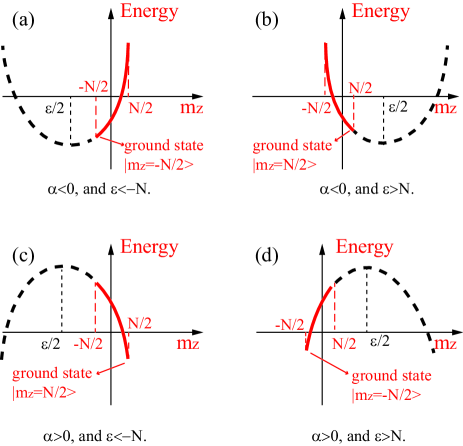
where the coefficients are , and . In which, the collective spins operator is , with the maximum total angular momentum ( is integer or half integer number). This isotropic LMG Hamiltonian can be solved exactly in the representation of because of the relations , where , and is the eigenstates of . In order to describe the physics more visually, in Fig. 2 we show the analysis graphics for the ground states of the isotropy LMG Hamiltonian in different conditions.
As shown in Fig. 2(a) and (b), when , , and because of the symmetry breaking , there must be a unique ground state for Eq. (14), and the result is shown in the first row of TABLE.II, with and . Here and . On the other hand, if we set and , we can also give a convincing interpretation of the ground state for according to Fig. 2(c) and (d). Then we can get the unique ground state for Eq. (14) in the second row of TABLE.II, with and .
By setting the parameters as the second and third rows in TABLE.I, we can also get the simple (one-axis twisting) LMG Hamiltonian
| (15) |
where the parameters are , , , , and .
| (16) |
with the parameters , , , , and .
According to Eq. (15) and Eq. (16), when we change the sign of from the negative value to the positive one, the collective spin system correspondingly undergoes the phase transition from the ferromagnetic interactions (FI) to the antiferromagnetic interactions (AFI). These transitions can also lead to the collective NV spins’ ground-state transitions shown in TABLE. II. When , Eqs. (15) and (16) are the Hamiltonians for describing the FI, whose ground states are double degenerate ones according to the third and the fifth rows in TABLE. II, with the expressions and . Here and . On the contrary, if we set , we can have the Hamiltonian for AFI, and obtain the ground states corresponding to the fourth and the sixth rows in TABLE. II, i.e., ( is even) and ( is odd).
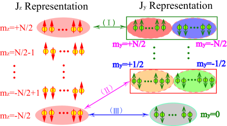
In this work, we focus on the generation of the multiparticle entangled states through adiabatically steering the Hamiltonian from the isotropic type to the one-axis twisting one . The essential criteria for this scheme is that we need to keep all spins in the ground states during the dynamical evolution process. It is necessary to determine the slowly varying functions of the Rabi frequencies versus the evolution time. Then we tune the parameters slowly enough to maintain the adiabatic conditions , in which is the characteristic time for the transfer process, and is the energy difference between the ground state and the next excited state. According to the discussion in Ref. Mølmer and Sørensen (1999), this adiabaticity constraints will not change as we increase the number of particles up to 50. In our scheme, the number of the NV centers have been limited in N 10, as a result, the adiabaticity constraints will be valid. We consider three different schemes: case I, , ; case II, , and is odd; case III, , and is even. These three different types of adiabatic processes are shown in Fig. 3.
For case I, we set the coupling parameters to satisfy , , , and , and assume that Eq. (14) is the initial Hamiltonian in this hybrid quantum system, which corresponds to the first row in TABLE. I. According to Fig. 2(b) and the first row in TABLE. II, we can analytically achieve the unique initial ground states for Eq. (14), which is the separable multiparticle state without any entanglement. With the adiabatic transfer process and , we can transform the LMG Hamiltonian from Eq. (14) into Eq. (15). As a result, we can achieve the adiabatic transfer process in this hybrid quantum system. Moreover, since the Hamiltonian for this type of transition corresponds to the FI, there is no need to discuss the odevity of the number of NV centers. Owing to the particular symmetry of the exchange of particles for this kind of LMG-type interactions as Eqs. (14) and (15), we can get the adiabatic ground-state transfer between the initial disentangled ground state and the final target entangled ground state,
| (17) |
Here corresponds to the -particle GHZ-type entangled state in the representation, and the total number of spins can sensitively influence on the entanglement due to the phase factor . For example, when , we can have .
For another case, according to the first row in TABLE. I and the second row in TABLE. II, we set the parameters as , , , and . Therefore, for Eq. (14), the initial ground state can be expressed as , which is also plotted in Fig. 2(d). Taking advantage of the same adiabatic transfer process and , we can also achieve the transfer process to prepare the entangled ground states. Since , the initial Hamiltonian is the form of FI, but the final Hamiltonian is the type of AI. In this adiabatic transfer process, the odevity of needs to be distinguished between odd (case II) and even (case III), as illustrated in Fig. 3.
In case II, and the total number of NV spins is odd. The ground states for the final Hamiltonian are two generate ground states as , which are both maximally entangled states. Moreover, owing to the symmetrical interactions for exchanging the particles, we can get the second adiabatic transition process in case II,
| (18) |
where is the -particle W-type maximally entangled state in the representation, with the total angular momentum for all the spins. Similarly, when , we can obtain and . Evidently, are both the W-type maximally entangled state in the representation.
For case III, and the total number of NV spins is even. With the final Hamiltonian , we have the unique nondegenerate ground state as , which is also the W-type maximally entangled state. Then we obtain the third adiabatic transition process in case III,
| (19) |
where is also the -particle W-type maximally entangled state in the representation, with the total angular momentum for all the NV spins. When , we have the target state as , which corresponds to the four-particle W-type maximally entangled state.
IV Numerical simulations
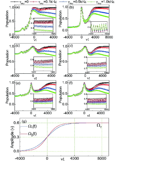
To confirm our theoretical schemes discussed above, we assume that the frequency of the NAMR is about MHz and the dephasing rates for all the NV spins are homogeneous . Then we make the numerical simulations through solving the master equation (13), and display the results for different cases in Fig. 4. In these numerical simulations, we have set the dephasing rate respectively as kHz, kHz, kHz, and kHz.
The adiabatic ground-state transfer process for case I is plotted in Fig. 4(a) and (b). We have assumed that the NV spins are initially prepared in the ground state and set the number of NV spins as . This adiabatic process corresponds to the transition of the FI LMG model between the isotropy type and the one-axis twisting type as shown in Fig. 3. We apply the slowly varying dichromatic microwave fields with the Rabi frequencies and according to Fig. 4(g), and obtain the dynamical evolution of the population for the target state .
In Fig. 4(a), the detuning is and the coupling is , while in Fig. 4(b) the detuning is and the coupling is . We find that the collective NV spins will be transferred to the GHZ state at the time . When the coupling strength between the NV centers and the NAMR decreases, as shown in Fig. 4(b), the time for reaching the target state will be much longer. Furthermore, we find that in ideal conditions the system can be steered into the target GHZ state with a fidelity equal to unity. However, when the spin dephasing effect is taken into account, the population in the target state decreases.
For case II and case III, the adiabatic state transfer schemes correspond to the transitions from the FI to the AFI as shown in Fig. 3. In these cases, the target states depend on the odd or even number of the NV spins. Therefore, for case II, we have set the odd number of NV spins as and assumed that the NV spins are initially prepared in the ground state . With the assistance of the slowly varying dichromatic microwave fields according to Fig. 4(g), we can acquire the dynamical evolution of the population for the target state in our numerical simulation.
As shown in Fig. 4(c)-(d), we set , in Fig. 4(c), and , in Fig. 4(d). We find that the collective NV spins will be transferred to the W-type entangled ground state when under different detunings. We can also find that the population of the target W-state can reach unity in ideal conditions, but less than unity in real conditions because of the dephasing effect.
While for case III, we have set the even number of NV spins as and assumed that the NV spins are also initially prepared in the ground state . With the assistance of the identical dichromatic microwave fields according to Fig. 4(g), we can also obtain the dynamical evolution of the population for the target state , as illustrated in Fig. 4(e) and (f). The parameters are chosen the same as those in Fig. 4(c) and (d). Obviously, in spite of the different detunings the collective four NV spins will be transferred to the W-type entangled ground state at the time . We also find that the NV spins can be steered into the target W-type state with a fidelity equal to unity in ideal conditions. However, when the spin dephasing effect is taken into account, the population in the target state decreases.
V Experimental imperfections
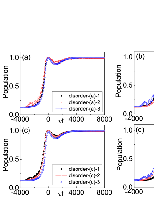
We now discuss the experimental imperfections. In this scheme, the experimental imperfections are mainly the physical disorder and the dispersion of the control parameters. Owing to the variations in the size and spacing of the magnetic tips and NV centers, and according to the discussion in Sec.II, the physical disorder is mainly caused by the inhomogeneous coupling between the NV centers and magnetic tips. We can make numerical simulations and display the effect of different disorder distributions on our scheme Janarek et al. (2018); Underwood et al. (2012); Ashhab (2015); de Abreu et al. (2018). We set , , and the slowly varying Rabi frequencies and . In Fig. 5, we plot the transfer efficiency under different disorder distributions. Moreover, according to the different values of , we consider four different cases (disorder-(a,b,c,d)) in Fig. 5: in Fig. 5(a), in Fig. 5(b), in Fig. 5(c), and in Fig. 5(d).
In our simulations, we take four spins as an example. In Fig. 5, we choose three different distributions for each disorder case. According to the numerical simulations as shown in Fig. 5 (a)-(d), we find that the collective NV spins will be transferred to the target ground state when the disorder is about of , and this transfer process is unaffected by these kinds of disorder.
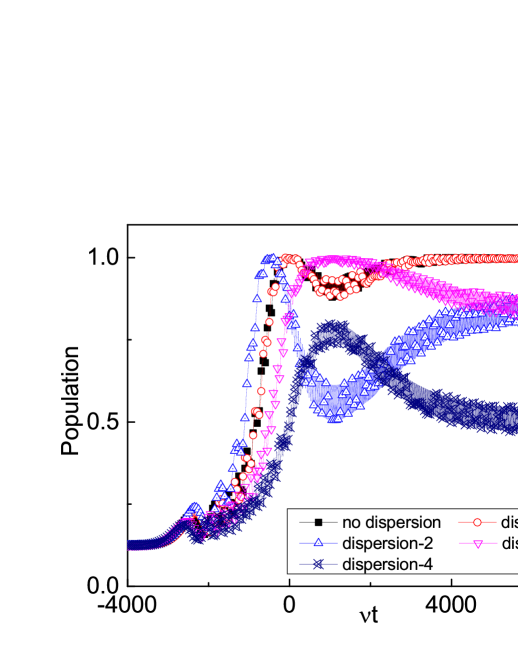
The dispersion caused by the experimental control parameters is another experimental imperfection. In this scheme, the dispersion mainly results from the dichromatic slowly varying Rabi frequencies and . We assume and , with the average value , and the dispersions . By setting , , we plot the dynamical evolution for the ground-state transfer efficiency in Fig. 6 under five different situations: {, }, {, }, {, }, {, }, and {, }.
As illustrated in Fig. 6, we find that the collective NV spins will be transferred to the target state with high efficiency when the dispersion satisfies . However, the transfer efficiency will decrease when the dispersion becomes larger. Hence, in order to prepare the target entangled state with high efficiency in this scheme, the dispersion of the control parameters should satisfy .
VI The feasibility of this scheme
To examine the feasibility of our scheme in realistic experiment, we now discuss the relevant experimental parameters. For realistic conditions, the frequency for high- () NAMR is about MHz, with the number of NV spins , we can obtain the magnetic coupling strength between the NAMR and the NV centers satisfies MHz. The Rabi frequency is about MHz and the detuning satisfies MHz. Assuming an environmental temperature mK in a dilution refrigerator, the thermal phonon number is about , and we can get the effective damping rate of NAMR is about Hz. Comparing with the effective couplings MHz and MHz, we can discard the effect of the NAMR’s damping rate in our numerical simulation Sidles et al. (1995); Liu et al. (2014); Li et al. (2015); Ekinci and Roukes (2005); Yang et al. (2000). Based on these parameters above, the time for transfer the NV spins’ ground state adiabatically from separate state to maximal entangled state will be about in this scheme. On the other hand, the relaxation time of the NV spin triplet ranging from milliseconds at room temperature to several seconds at low temperature has been reported. In general, the single NV spin decoherence in diamond is mainly caused by the coupling of the surrounding electron or nuclear spins, such as the electron spins P1 centers, the nuclear spins spins and spins Naydenov et al. (2011); Zhao et al. (2012). In type-Ib diamond samples, the free-induction decay of the NV center spin in an electron spin bath (P1 centers) can be neglected, and in high-purity type-IIa samples, the decay time caused by the electron spin bath will exceed one millisecond Naydenov et al. (2011); Zhao et al. (2012, 2014). The coupling to the host nuclear spin(MHz), induces the substantial coherent off-resonance errors, and these errors have been solved experimentally Ryan et al. (2010). For NV centers in diamond with natural abundance of , the decoherence will be dominated by the hyperfine interaction with the nuclear spins, which mainly form the nuclear spin bath Zhao et al. (2011a); Childress et al. (2006); Zhao et al. (2011b). With the development of the dynamical decoupling techniques Viola et al. (1999); Witzel and Sarma (2007); Yao et al. (2007); Uhrig (2007); Hason et al. (2008); Yang and Liu (2008); West et al. (2010); Zhao et al. (2011b); Biercuk et al. (2009); Du et al. (2009); Taylor et al. (2008); Takahashi et al. (2008); Stanwix et al. (2010); Zhao et al. (2011c), the dephasing time of a single NV center in diamond can be more than ms Balasubramanian et al. (2009); Lange et al. (2010); Shim et al. (2012). Thus, the coherence time is sufficient for achieving the desired NV spins entangled ground state.
VII Conclusion
In summary, we have proposed an efficient protocol for entangling the NV spins with the assistance of a high- NAMR and dichromatic classical microwave driving fields. In this protocol, we can not only acquire the collective LMG type interactions for NV spins (), but also steer the LMG Hamiltonian adiabatically from the isotropic type to the simple (one-axis twisting) type by tuning the Rabi frequencies slowly enough to maintain the NV spins in the ground state. As a result, the collective NV spins will undergo ground state transitions, which allows us to obtain the adiabatic channels between the initial separate ground state and the final entangled ground state. In this work, we have made the analytical discussions and numerical simulations on three different types of adiabatic processes for cases I, II, and III. We can acquire the GHZ-type maximally entangled NV spin ground state in case I, and the W-type ground states in cases II and III under realistic conditions.
Acknowledgments
References
- Wootters (1998) W. K. Wootters, Phys. Rev. Lett. 80, 2245 (1998).
- Vedral (2002) V. Vedral, Rev. Mod. Phys. 74, 197 (2002).
- Horodecki et al. (2009) R. Horodecki, P. Horodecki, M. Horodecki, and K. Horodecki, Rev. Mod. Phys. 81, 865 (2009).
- Sørensen and Mølmer (1999) A. Sørensen and K. Mølmer, Phys. Rev. Lett. 82, 1971 (1999).
- James (1998) D. F. V. James, Appl. Phys. B 66, 181 (1998).
- Raussendorf and Briegel (2001) R. Raussendorf and H. J. Briegel, Phys. Rev. Lett. 86, 5188 (2001).
- Dakić and Radonjić (2017) B. Dakić and M. Radonjić, Phys. Rev. Lett. 119, 090401 (2017).
- Cirac and Zoller (1995) J. I. Cirac and P. Zoller, Phys. Rev. Lett. 74, 4091 (1995).
- Zheng (2001) S.-B. Zheng, Phys. Rev. Lett. 87, 230404 (2001).
- Mølmer and Sørensen (1999) K. Mølmer and A. Sørensen, Phys. Rev. Lett. 82, 1835 (1999).
- Unanyan et al. (2001) R. G. Unanyan, N. V. Vitanov, and K. Bergmann, Phys. Rev. Lett. 87, 137902 (2001).
- Unanyan and Fleischhauer (2003) R. G. Unanyan and M. Fleischhauer, Phys. Rev. Lett. 90, 133601 (2003).
- Morrison and Parkins (2008) S. Morrison and A. S. Parkins, Phys. Rev. Lett. 100, 040403 (2008).
- Møller et al. (2008) D. Møller, L. B. Madsen, and K. Mølmer, Phys. Rev. Lett. 100, 170504 (2008).
- Zhang and Duan (2013) Z. Zhang and L.-M. Duan, Phys. Rev. Lett. 111, 180401 (2013).
- Reiter et al. (2016) F. Reiter, D. Reeb, and A. S. Sørensen, Phys. Rev. Lett. 117, 040501 (2016).
- Armata et al. (2017) F. Armata, G. Calajo, T. Jaako, M. S. Kim, and P. Rabl, Phys. Rev. Lett. 119, 183602 (2017).
- Ashhab et al. (2008) S. Ashhab, A. O. Niskanen, K. Harrabi, Y. Nakamura, T. Picot, P. C. de Groot, C. J. P. M. Harmans, J. E. Mooij, and F. Nori, Phys. Rev. B 77, 014510 (2008).
- Li et al. (2017) X.-X. Li, P.-B. Li, S.-L. Ma, and F.-L. Li, Sci. Rep. 7, 14116 (2017).
- Yang et al. (2012) C.-P. Yang, Q.-P. Su, and S. Han, Phys. Rev. A 86, 022329 (2012).
- Yang et al. (2013) C.-P. Yang, Q.-P. Su, S.-B. Zheng, and S. Han, Phys. Rev. A 87, 022320 (2013).
- Häffner et al. (2005) H. Häffner, W. Hänsel, C. F. Roos, J. Benhelm, D. Chekalkar, M. Chwalla, T. Körber, U. D. Rapol, M. Riebe, and P. O. Schmidt, Nature 438, 643 (2005).
- Meekhof et al. (1996) D. M. Meekhof, C. Monroe, B. E. King, W. M. Itano, and D. J. Wineland, Phys. Rev. Lett. 76, 1796 (1996).
- Barontini et al. (2015) G. Barontini, L. Hohmann, F. Haas, J. Estéve, and J. Reichel, Science 349, 1317 (2015).
- Neumann et al. (2008) P. Neumann, N. Mizuochi, F. Rempp, P. Hemmer, H. Watanabe, S. Yamasaki, V. Jacques, T. Gaebel, F. Jelezko, and J. Wrachtrup, Science 320, 1326 (2008).
- Sackett et al. (2000) C. A. Sackett, D. Kielpinski, B. E. King, C. Langer, V. Meyer, C. J. Myatt, M. Rowe, Q. A. Turchette, W. M. Itano, and D. J. Wineland, Nature 404, 256 (2000).
- Zhu et al. (2011) X. Zhu, S. Saito, A. Kemp, K. Kakuyanagi, S. Karimoto, H. Nakano, W. J. Munro, Y. Tokura, M. S. Everitt, and K. Nemoto, Nature 478, 221 (2011).
- Johnson et al. (2017) K. G. Johnson, J. D. Wongcampos, B. Neyenhuis, J. Mizrahi, and C. Monroe, Nat. Commun. 8, 697 (2017).
- Xiang et al. (2013a) Z.-L. Xiang, S. Ashhab, J. Q. You, and F. Nori, Rev. Mod. Phys. 85, 623 (2013a).
- Rabl et al. (2006) P. Rabl, D. DeMille, J. M. Doyle, M. D. Lukin, R. J. Schoelkopf, and P. Zoller, Phys. Rev. Lett. 97, 033003 (2006).
- Peng et al. (2012) Z. H. Peng, Y.-x. Liu, Y. Nakamura, and J. S. Tsai, Phys. Rev. B 85, 024537 (2012).
- Xiang et al. (2013b) Z.-L. Xiang, X.-Y. Lü, T.-F. Li, J. Q. You, and F. Nori, Phys. Rev. B 87, 144516 (2013b).
- Lü et al. (2013) X.-Y. Lü, Z.-L. Xiang, W. Cui, J. Q. You, and F. Nori, Phys. Rev. A 88, 012329 (2013).
- Song et al. (2017) W. Song, W. Yang, J. An, and M. Feng, Opt. Express 25, 19226 (2017).
- Houck et al. (2016) A. A. Houck, H. E. Türeci, and J. Koch, Nat. Phys. 8, 292 (2016).
- Buluta et al. (2012) I. Buluta, S. Ashhab, and F. Nori, Rep. Prog. Phys. 74, 104401 (2012).
- You and Nori (2005) J. Q. You and F. Nori, Phys. Today 58, 42 (2005).
- Hong et al. (2012) S. Hong, M. S. Grinolds, P. Maletinsky, R. L. Walsworth, M. D. Lukin, and A. Yacoby, Nano. Lett. 12, 3920 (2012).
- Doherty et al. (2013) M. W. Doherty, N. B. Manson, P. Delaney, F. Jelezko, J. Wrachtrup, and L. C. L. Hollenberg, Phys. Rep. 528, 1 (2013).
- Maze et al. (2011) J. Maze, A. Gali, E. Togan, Y. Chu, A. Trifonov, E. Kaxiras, and M. Lukin, New J. Phys. 13, 780 (2011).
- Kubo et al. (2010) Y. Kubo, F. R. Ong, P. Bertet, D. Vion, V. Jacques, D. Zheng, A. Dréau, J.-F. Roch, A. Auffeves, F. Jelezko, J. Wrachtrup, M. F. Barthe, P. Bergonzo, and D. Esteve, Phys. Rev. Lett. 105, 140502 (2010).
- Kubo et al. (2011) Y. Kubo, C. Grezes, A. Dewes, T. Umeda, J. Isoya, H. Sumiya, N. Morishita, H. Abe, S. Onoda, T. Ohshima, V. Jacques, A. Dréau, J.-F. Roch, I. Diniz, A. Auffeves, D. Vion, D. Esteve, and P. Bertet, Phys. Rev. Lett. 107, 220501 (2011).
- MacQuarrie et al. (2013) E. R. MacQuarrie, T. A. Gosavi, N. R. Jungwirth, S. A. Bhave, and G. D. Fuchs, Phys. Rev. Lett. 111, 227602 (2013).
- Golter et al. (2016a) D. A. Golter, T. Oo, M. Amezcua, K. A. Stewart, and H. Wang, Phys. Rev. Lett. 116, 143602 (2016a).
- Teissier et al. (2014) J. Teissier, A. Barfuss, P. Appel, E. Neu, and P. Maletinsky, Phys. Rev. Lett. 113, 020503 (2014).
- Bar-Gill et al. (2013) N. Bar-Gill, L. M. Pham, A. Jarmola, D. Budker, and R. L. Walsworth, Nat. Commun. 4, 1743 (2013).
- Doherty et al. (2012) M. W. Doherty, F. Dolde, H. Fedder, F. Jelezko, J. Wrachtrup, N. B. Manson, and L. C. L. Hollenberg, Phys. Rev. B 85, 205203 (2012).
- Golter and Wang (2014) D. A. Golter and H. Wang, Phys. Rev. Lett. 112, 116403 (2014).
- Golter et al. (2014) D. A. Golter, T. K. Baldwin, and H. Wang, Phys. Rev. Lett. 113, 237601 (2014).
- Golter et al. (2016b) D. A. Golter, T. Oo, M. Amezcua, I. Lekavicius, K. A. Stewart, and H. Wang, Phys. Rev. X 6, 041060 (2016b).
- Dai and Kwek (2012) L. Dai and L. C. Kwek, Phys. Rev. Lett. 108, 066803 (2012).
- Sipahigil et al. (2012) A. Sipahigil, M. L. Goldman, E. Togan, Y. Chu, M. Markham, D. J. Twitchen, A. S. Zibrov, A. Kubanek, and M. D. Lukin, Phys. Rev. Lett. 108, 143601 (2012).
- Yang et al. (2011) W. L. Yang, Y. Hu, Z. Q. Yin, Z. J. Deng, and M. Feng, Phys. Rev. A 83, 022302 (2011).
- Xia and Twamley (2016) K. Xia and J. Twamley, Phys. Rev. B 94, 205118 (2016).
- Li et al. (2016) P.-B. Li, Z.-L. Xiang, P. Rabl, and F. Nori, Phys. Rev. Lett. 117, 015502 (2016).
- Bennett et al. (2013) S. D. Bennett, N. Y. Yao, J. Otterbach, P. Zoller, P. Rabl, and M. D. Lukin, Phys. Rev. Lett. 110, 156402 (2013).
- Li and Nori (2018) P.-B. Li and F. Nori, Phys. Rev. Applied 10, 024011 (2018).
- Amsüss et al. (2011) R. Amsüss, C. Koller, T. Nöbauer, S. Putz, S. Rotter, K. Sandner, S. Schneider, M. Schramböck, G. Steinhauser, H. Ritsch, J. Schmiedmayer, and J. Majer, Phys. Rev. Lett. 107, 060502 (2011).
- You et al. (2014) J.-B. You, W. L. Yang, Z.-Y. Xu, A. H. Chan, and C. H. Oh, Phys. Rev. B 90, 195112 (2014).
- Marcos et al. (2010) D. Marcos, M. Wubs, J. M. Taylor, R. Aguado, M. D. Lukin, and A. S. Sørensen, Phys. Rev. Lett. 105, 210501 (2010).
- Zou et al. (2014) L. J. Zou, D. Marcos, S. Diehl, S. Putz, J. Schmiedmayer, J. Majer, and P. Rabl, Phys. Rev. Lett. 113, 023603 (2014).
- Zhou et al. (2017) Y. Zhou, S.-L. Ma, B. Li, X.-X. Li, F.-L. Li, and P.-B. Li, Phys. Rev. A 96, 062333 (2017).
- Dolde et al. (2011) F. Dolde, H. Fedder, M. W. Doherty, T. Nöbauer, F. Rempp, G. Balasubramanian, T. Wolf, F. Reinhard, L. C. L. Hollenberg, F. Jelezko, and J. Wrachtrup, Nat. Phys. 7, 459 (2011).
- Albrecht et al. (2013) A. Albrecht, A. Retzker, F. Jelezko, and M. B. Plenio, New J. Phys. 15, 83014 (2013).
- Rabl et al. (2009) P. Rabl, P. Cappellaro, M. V. G. Dutt, L. Jiang, J. R. Maze, and M. D. Lukin, Phys. Rev. B 79, 041302 (2009).
- Xu et al. (2009) Z. Y. Xu, Y. M. Hu, W. L. Yang, M. Feng, and J. F. Du, Phys. Rev. A 80, 022335 (2009).
- Ma et al. (2017) Y. Ma, T. M. Hoang, M. Gong, T. Li, and Z.-q. Yin, Phys. Rev. A 96, 023827 (2017).
- Rabl et al. (2010) P. Rabl, S. J. Kolkowitz, F. H. L. Koppens, J. G. E. Harris, P. Zoller, and M. D. Lukin, Nat. Phys. 6, 602 (2010).
- Lipkin et al. (1965) H. Lipkin, N. Meshkov, and A. Glick, Nucl. Phys. 62, 188 (1965).
- Janarek et al. (2018) J. Janarek, D. Delande, and J. Zakrzewski, Phys. Rev. B 97, 155133 (2018).
- Underwood et al. (2012) D. L. Underwood, W. E. Shanks, J. Koch, and A. A. Houck, Phys. Rev. A 86, 023837 (2012).
- Ashhab (2015) S. Ashhab, Phys. Rev. A 92, 062305 (2015).
- de Abreu et al. (2018) B. R. de Abreu, U. Ray, S. A. Vitiello, and D. M. Ceperley, Phys. Rev. A 98, 023628 (2018).
- James and Jerke (2012) D. F. V. James and J. Jerke, Can. J. Phys. 85, 625 (2012).
- Tsomokos et al. (2008) D. I. Tsomokos, S. Ashhab, and F. Nori, New J. Phys. 10, 113020 (2008).
- Sidles et al. (1995) J. A. Sidles, J. L. Garbini, K. J. Bruland, D. Rugar, O. Züger, S. Hoen, and C. S. Yannoni, Rev. Mod. Phys. 67, 249 (1995).
- Liu et al. (2014) Y.-C. Liu, X. Luan, H.-K. Li, Q. Gong, C. W. Wong, and Y.-F. Xiao, Phys. Rev. Lett. 112, 213602 (2014).
- Li et al. (2015) P.-B. Li, Y.-C. Liu, S.-Y. Gao, Z.-L. Xiang, P. Rabl, Y.-F. Xiao, and F.-L. Li, Phys. Rev. Applied 4, 044003 (2015).
- Ekinci and Roukes (2005) K. L. Ekinci and M. L. Roukes, Rev. Sci. Instrum. 76, 061101 (2005).
- Yang et al. (2000) J. Yang, T. Ono, and M. Esashi, Appl. Phys. Lett. 77, 3860 (2000).
- Naydenov et al. (2011) B. Naydenov, F. Dolde, L. T. Hall, C. Shin, H. Fedder, L. C. L. Hollenberg, F. Jelezko, and J. Wrachtrup, Phys. Rev. B 83, 081201 (2011).
- Zhao et al. (2012) N. Zhao, S.-W. Ho, and R.-B. Liu, Phys. Rev. B 85, 115303 (2012).
- Zhao et al. (2014) N. Zhao, J. Wrachtrup, and R.-B. Liu, Phys. Rev. A 90, 032319 (2014).
- Ryan et al. (2010) C. A. Ryan, J. S. Hodges, and D. G. Cory, Phys. Rev. Lett. 105, 200402 (2010).
- Zhao et al. (2011a) N. Zhao, W. Yang, S. W. Ho, J. L. Hu, J. T. K. Wan, and R. B. Liu, AIP Conference Proceedings 1399, 697 (2011a).
- Childress et al. (2006) L. Childress, M. V. Gurudev Dutt, J. M. Taylor, A. S. Zibrov, F. Jelezko, J. Wrachtrup, P. R. Hemmer, and M. D. Lukin, Science 314, 281 (2006).
- Zhao et al. (2011b) N. Zhao, Z.-Y. Wang, and R.-B. Liu, Phys. Rev. Lett. 106, 217205 (2011b).
- Viola et al. (1999) L. Viola, E. Knill, and S. Lloyd, Phys. Rev. Lett. 82, 2417 (1999).
- Witzel and Sarma (2007) W. M. Witzel and S. D. Sarma, Phys. Rev. Lett. 98, 077601 (2007).
- Yao et al. (2007) W. Yao, R.-B. Liu, and L. J. Sham, Phys. Rev. Lett. 98, 077602 (2007).
- Uhrig (2007) G. S. Uhrig, Phys. Rev. Lett. 98, 100504 (2007).
- Hason et al. (2008) R. Hason, V. V. Dobrovitski, A. E. Feiguin, O. Gywat, and D. D. Awschalom, Science 320, 352 (2008).
- Yang and Liu (2008) W. Yang and R.-B. Liu, Phys. Rev. Lett. 101, 180403 (2008).
- West et al. (2010) J. R. West, D. A. Lidar, B. H. Fong, and M. F. Gyure, Phys. Rev. Lett. 105, 230503 (2010).
- Biercuk et al. (2009) M. J. Biercuk, M. J. Biercuk, H. Uys, A. P. VanDevender, N. Shiga, W. M. Itano, and J. J. Bollinger, Nature 458, 996 (2009).
- Du et al. (2009) J. Du, X. Rong, N. Zhao, Y. Wang, J. Yang, and R. B. Liu, Nature 461, 1265 (2009).
- Taylor et al. (2008) J. M. Taylor, P. Cappellaro, L. Childress, L. Jiang, D. Budker, P. R. Hemmer, A. Yacoby, R. Walsworth, and M. D. Lukin, Nat. Phys. 4, 810 (2008).
- Takahashi et al. (2008) S. Takahashi, R. Hanson, J. van Tol, M. S. Sherwin, and D. D. Awschalom, Phys. Rev. Lett. 101, 047601 (2008).
- Stanwix et al. (2010) P. L. Stanwix, L. M. Pham, J. R. Maze, D. Le Sage, T. K. Yeung, P. Cappellaro, P. R. Hemmer, A. Yacoby, M. D. Lukin, and R. L. Walsworth, Phys. Rev. B 82, 201201 (2010).
- Zhao et al. (2011c) N. Zhao, J. L. Hu, S. W. Ho, J. T. K. Wan, and R. B. Liu, Nature Nanotechnology 6, 242 (2011c).
- Balasubramanian et al. (2009) G. Balasubramanian, P. Neumann, D. Twitchen, M. Markham, R. Kolesov, N. Mizuochi, J. Isoya, J. Achard, J. Beck, and J. Tissler, Nature Materials 8, 383 (2009).
- Lange et al. (2010) G. D. Lange, Z. H. Wang, D. Ristè, V. V. Dobrovitski, and R. Hanson, Science 330, 60 (2010).
- Shim et al. (2012) J. H. Shim, I. Niemeyer, J. Zhang, and D. Suter, Epl 99, 40004 (2012).
- Johansson et al. (2012) J. R. Johansson, P. D. Nation, and F. Nori, Comput. Phys. Commun. 183, 1760 (2012).
- Johansson et al. (2013) J. R. Johansson, P. D. Nation, and F. Nori, Comput. Phys. Commun. 184, 1234 (2013).