Knowledge-Aided Normalized Iterative Hard Thresholding Algorithms and Applications to Sparse Reconstruction

Abstract

This paper deals with the problem of sparse recovery often found in compressive sensing applications exploiting a priori knowledge. In particular, we present a knowledge-aided normalized iterative hard thresholding (KA-NIHT) algorithm that exploits information about the probabilities of nonzero entries. We also develop a strategy to update the probabilities using a recursive KA-NIHT (RKA-NIHT) algorithm, which results in improved recovery. Simulation results illustrate and compare the performance of the proposed and existing algorithms.

Index Terms—  compressed sensing, iterative hard thresholding, prior information, probability estimation, sparse recovery

1 Introduction

Sparse signal recovery problems are among the fundamental problems addressed in compressed sensing (CS) [1, 2, 3, 4, 5, 6, 7, 8] which have been successfully utilized in many areas such as image processing [9], wireless sensor networks [10], and face recognition [11]. Most often this problem refers to recovering a sparse signal $\mathbf{x}$ from its linear measurements:

$$\mathbf{y=Ax+e},$$ (1)

where $\|\mathbf{x}\|_{0}\leq K$ (here $\|\cdot\|_{0}$ counts the number of non-zero elements), $\mathbf{A}\in\Re^{M\times N}$ with $M\leq N$, and $\mathbf{e}{\in\Re^{M\times 1}}$ is the noise which is modeled by independent and identically distributed Gaussian random variables with zero mean and variance $\sigma^{2}$.

Although most of the signals are not directly sparse, they can be sparsely represented by a well-chosen dictionary $\mathbf{\Psi}\in\Re^{L\times N}$ with $L\leq N$. A signal $\mathbf{s}$ is said to be sparsely represented under $\mathbf{\Psi}$ if

$$\mathbf{s=\Psi x},$$ (2)

Typical examples of the dictionaries include the Fourier matrix for frequency-sparse signals, a multiband modulated Discrete Prolate Spheroidal Sequences (DPSSs) dictionary for sampled multiband signals [12] and one learned from the training data [13]. In CS, a sensing matrix $\mathbf{\Phi}\in\Re^{M\times L},M\leq L$ [14, 15] is utilized to capture most of the information contained in the signal $\mathbf{s}$ that can be sparsely represented under $\mathbf{\Psi}$. Thus, for the measurement in (1) we have $\mathbf{A=\Phi\Psi}$. Algorithms for finding the sparse vector $\mathbf{x}$ from the measurement $\mathbf{y}$ include the orthogonal matching pursuit (OMP) [16], basic pursuit (BP) [17], least absolute shrinkage and selection operator (LASSO) [18], iterative hard thresholding (IHT)[19], dichotomous coordinate descent (DCD)-based algorithm [20], adaptive approaches [21, 22, 23, 24, 25, 26, 27, 28, 29, 30, 31, 32, 33, 34, 35, 36, 37, 38, 39] and $\ell_{1}$-homotopy [40, 41].

A sparse signal can be successfully recovered when both the values of the nonzero elements of $\mathbf{x}$ and their positions are accurately estimated. The use of a priori information about such values and their positions has been shown to provide improvements to the recovery task [42] - [43]. In particular, prior work [44] has exploited the probabilities of the nonzero elements to improve the recovery using the OMP algorithm. However, there has been no attempt so far to consider the improvement of other existing algorithms such as the normalized iterative hard theresholding (NIHT) [45] with the exploitation of prior knowledge. Therefore, we propose a knowledge-aided NIHT (KA-NIHT) algorithm and a recursive KA-NIHT (RKA-NIHT) algorithm, which can exploit prior information in the form of probabilities of nonzero entries. Note that the probabilities that have been used in [44] as a priori knowledge are fixed. However, in practice, such a precise knowledge can hardly be available. A more practical approach is to consider these probabilities just as educated guesses, and update them within the iterations using the RKA-NIHT algorithm. To this end, we propose the use of an adaptive set of probabilities and develop a recursive procedure to compute these probabilities over the iterations. Simulations show that the proposed KA-NIHT and RKA-NIHT algorithms outperform existing recovery techniques.

The organization of the remaining part of the paper is as follows. Some preliminary work is introduced in Section 2. Section 3 describes the proposed knowledge-aided algorithms using the initial probability vector and adjustment of the probability vector through a recursive method based on the NIHT algorithm. Section 4 presents and discusses simulation results. Section 5 gives the conclusion of our work.

2 Preliminary Work

In compressive sensing systems, a designer often employs a recovery algorithm to obtain a sparse solution. A recovery algorithm can be formulated as an optimization problem that can be written as:

$$\widehat{\mathbf{x}}=\arg\min_{\mathbf{x}:\|\mathbf{x}\|_{0}\leq K}\|\mathbf{y-Ax}\|_{2}^{2},$$ (3)

where $\|\cdot\|_{2}$ denotes the 2-norm of a vector, Thus, a sparse vector $\widehat{\mathbf{x}}$ should be found so that the error $\|\mathbf{y-Ax}\|_{2}^{2}$ is minimized under the $K$-sparsity constraint $\|\mathbf{x}\|_{0}\leq K$. In the following subsections, the NIHT algorithm and types of a priori information on the sparsity are introduced.

2.1 Normalized Iterative Hard Thresholding

Under the condition of the restricted isometry property [46], the sparse recovery can be obtained by using the NIHT algorithm [45]. In the NIHT algorithm, the cost function decreases in every iteration until the convergence. Let the solution vector be initialized as $\mathbf{x}^{0}=\mathbf{0}$. The following iterations ($l\geq 1$) are used in the NIHT algorithm:

$$\mathbf{x}_{l+1}=H_{K}(\mathbf{x}_{l}+\mu\mathbf{A}^{T}(\mathbf{y-Ax}_{l})),$$ (4)

where $H_{K}(\cdot)$ is an operator setting all elements of a vector to zero except for the K elements with the largest magnitudes. The step size $\mu$ is adapted to maximally minimize the error in every iteration:

$$\mu=\frac{\mathbf{g}_{\Lambda_{l}}^{T}\mathbf{g}_{\Lambda_{l}}}{\mathbf{g}_{\Lambda_{l}}^{T}\mathbf{A}_{\Lambda_{l}}^{T}\mathbf{A}_{\Lambda_{l}}\mathbf{g}_{\Lambda_{l}}},$$ (5)

where $\Lambda_{l}$ is the support of $\mathbf{x}_{l}$ and $\mathbf{g}=\mathbf{A}^{T}(\mathbf{y-Ax}_{l})$ is the negative gradient of $\|\mathbf{y-Ax}\|_{2}^{2}$.

2.2 A priori information on sparsity

The NIHT algorithm exploits a priori information o the sparsity of the solution in the form of the number of non-zero elements $K$. The performance of a sparse recovery algorithm can be improved if extra a priori information on the sparsity of the solution is available. Let a sparse signal $\mathbf{x}=[x_{1},\cdots,x_{N}]^{T}$ be generated using the following rule. The $i$-th entry of of $\mathbf{x}$ is given by

$$x_{i}=w_{i}\vartheta_{i},$$ (6)

where $w_{i}$ is a deterministic non-zero value, and $\vartheta_{i}\in\{0,1\}$ is a random binary variable used to decide whether the entry is zero or non-zero according to a probability distribution. The probability for $\vartheta_{i}=1$ is denoted as $p_{i}$, and the random variable $\{\vartheta_{i}\}_{i=1}^{N}$ are assumed independent. The support of $\mathbf{x}$ is given by $\Lambda=\{i|\vartheta_{i}=1\}$. In [44], OMP [16], BP [17] and LASSO [18] algorithms are extended to exploit a priori information in the form of the probability distribution $\mathbf{p}=[p_{1},\cdots,p_{N}]^{T}$ which are named as Log-Weighted OMP (LW-OMP), Log-Weighted BP (LW-BP), Log-Weighted LASSO (LW-LASSO), respectively. The results show that excellent sparse recovery can be achieved if the probability distribution is sufficiently non-uniform, especially using LW-OMP algorithm. Therefore below we will use it as a benchmark for comparison with our algorithm.

The goal of this paper is to propose an efficient algorithm to estimate $\mathbf{x}$ from the observation $\mathbf{y}$ using $\mathbf{p}=[p_{1},\cdots,p_{N}]^{T}$ as prior probabilities based on the NIHT algorithm.

3 Proposed Reconstruction Algorithms

The NIHT algorithm according to (4) selects the support elements with the highest magnitudes. With such strategy, it is possible that non-zero elements with low magnitudes as missed. By exploiting the prior probabilities $\mathbf{p}=[p_{1},\cdots,p_{N}]^{T}$ the support estimate can be made more accurate and consequently the performance of sparse recovery improved.

We propose to recover the support in every iteration of the NIHT algorithm using the following operation:

$$\Lambda=\sup[S_{K}(|\mathbf{x}+\mu\mathbf{g}|+\alpha\log(\mathbf{p}))],$$ (7)

where $S_{K}(\cdot)$ is an operator to sort elements of a vector in descending order, sets last $(N-K)$ elements to zero, and return the elements back to the original order. The operator $\sup[\cdot]$ extracts positions of non-zero elements. Note that the notation $|\mathbf{x}+\mu\mathbf{g}|$ means element-wise magnitudes of the vector elements. Similarly, $\log(\mathbf{p})$ means $\log$ of each element of vector $\mathbf{p}$. The term $\log(\mathbf{p})$ introduces a penalty in the iterations. If $\alpha=0$, then we arrive at the NIHT algorithm. If $\alpha>0$, then for a high $p_{i}$ (close to one) the penalty is small, while for a small $p_{i}$ the penalty is high. As a result, if it is a priori know that the probability of appearance of the $i$-th element $p_{i}$ is low, it is unlikely that it would be selected into the support $\Lambda$. The parameter $\alpha$ controls the tradeoff between the importance of the current magnitude $|x_{i}+\mu g_{i}|$ of an element and its a priori probability $p_{i}$. The modification of the NIHT algorithm that exploits the support estimate according to (7) is named KA-NIHT.

Note that in the KA-NIHT algorithm, the a priori probabilities $\mathbf{p}$ are fixed. However, in practice, such a precise knowledge can hardly be available. A more practical approach is to consider these probabilities just as educated guesses, and update them within the iterations using the RKA-NIHT algorithm as described below.

In the RKA-NIHT algorithm, the support estimate (7) is replaced with the estimate:

$$\Lambda=\sup[S_{K}(|\mathbf{x}+\mu\mathbf{g}|+\alpha\log(\mathbf{q}))],$$ (8)

when the vector $\mathbf{q}=\mathbf{p}$ at the first iteration and it is updated recursively at the following iterations as:

$$\mathbf{q}_{\Lambda}\leftarrow\mathbf{q}_{\Lambda}+\beta\mathbf{p}_{\Lambda}.$$ (9)

Here we denote $\mathbf{q}_{\Lambda}$ a vector which is obtained from the vector $\mathbf{q}$ by only keeping elements on the support $\Lambda$. The parameter $\beta$ is a tuning parameter which is selected according to the experiments.

The steps of the RKA-NIHT algorithm are summarized as follows.

  Algorithm: RKA-NIHT   Input: Data vector $\mathbf{y}\in\Re^{M\times 1}$, compressed matrix $\mathbf{A}\in\Re^{M\times N}$, the sparsity $K$ is known. The probability vector is $\mathbf{p}$. The iteration number is $I$. $c,\kappa,\beta$ are constants.

Initialization: the solution vector $\mathbf{x}_{0}=\mathbf{0}$, and

$$\mathbf{x}_{1}=H_{K}(\mathbf{A}^{T}\mathbf{y}),$$

$\Lambda_{1}=\sup(\mathbf{x}_{1})$, $l=1$; $\mathbf{q}\leftarrow\mathbf{p}$.

Repeat until $l>I$:

Step 1: $\mathbf{g}_{l}=\mathbf{A}^{\cal T}(\mathbf{y}-\mathbf{Ax}_{l})$

Step 2: $\mu_{l}=\frac{\mathbf{g}^{T}_{\Lambda_{l}}\mathbf{g}_{\Lambda_{l}}}{\mathbf{g}^{T}_{\Lambda_{l}}\mathbf{A}^{T}_{\Lambda_{l}}\mathbf{A}_{\Lambda_{l}}\mathbf{A}_{\Lambda_{l}}}$

Step 3: $\Lambda_{l+1}=\sup[S_{K}(|\mathbf{x}_{l}+\mu_{l}\mathbf{g}_{l}|+\alpha\log(\mathbf{q}))]$

Step 4: $\hat{\mathbf{x}}_{l+1}=(\mathbf{x}_{l}+\mu_{l}\mathbf{g}_{l})_{\Lambda_{l+1}}$

Step 5: If $\Lambda_{l+1}=\Lambda_{l}$ then $\mathbf{x}_{l+1}=\hat{\mathbf{x}}_{l+1}$

else $\varrho=(1-c)(\|\hat{\mathbf{x}}_{l+1}-\mathbf{x}_{l}\|^{2}_{2})/(\|\mathbf{A}(\hat{\mathbf{x}}_{l+1}-\mathbf{x}_{l})\|^{2}_{2})$

if $\mu_{l}\geq\varrho$ repeat until $\mu_{l}\leq\varrho$

$\mu_{l}\leftarrow\mu_{l}/(\kappa(1-c))$

$\Lambda_{l+1}=\sup[S_{K}(|\mathbf{x}_{l}+\mu_{l}\mathbf{g}_{l}|+\alpha\log(\mathbf{q}))]$

$\hat{\mathbf{x}}_{l+1}=(\mathbf{x}_{l}+\mu_{l}\mathbf{g}_{l})_{\Lambda_{l+1}}$

$\mathbf{x}_{l+1}=\hat{\mathbf{x}}_{l+1}$

Step 6: Update $\mathbf{q}$:

$\mathbf{q}_{\Lambda_{l+1}}\leftarrow\mathbf{q}_{\Lambda_{l+1}}+\beta\mathbf{p}_{\Lambda_{l+1}}$

Step 7: $l=l+1$

Output: $\widehat{\mathbf{x}}=\mathbf{x}_{l}$

 

The KA-NIHT algorithm is the particular case of the algorithm RKA-NIHT when step 6 is removed.

The computational complexity of NIHT, KA-NIHT and RKA-NIHT per iteration is calculated and shown in Table 1.

Table 1: Computational complexity of three algorithms per iteration.

.

	Additions	Multiplications	Comparison
NIHT	$KM+K+2N+3MN+M-5$	$KM+K+2N+3MN+2M+3$	$2NlogN+1$
KA-NIHT	$KM+K+5N+2.75MN-2.5$	$KM+K+2.5N+2.75MN+1.75M+0.75$	$2.75NlogN+1.75K+0.75$
RKA-NIHT	$KM+2K+2.6N+2.4MN-1.8$	$KM+2K+1.8N+2.4MN+1.4M+0.4$	$2.75NlogN+1.75K+0.75$

4 Simulation Results

In this section, we investigate the performance of OMP [16], LW-OMP [44], NIHT [45], KA-NIHT, RKA-NIHT and Oracle NIHT algorithms for various $M$ and noise variance $\sigma^{2}$ with $N=240$, and $S=1000$ simulation trials.

The values $\{w_{i}\}_{i=1}^{N}$ in (6) are drawn from a Gaussian distribution $N(0,1)$. The support probabilities are modeled as follows. Elements of $\mathbf{x}$ are divided into $G$ groups. The proportions $h_{n}$ of elements in the groups are different, but $\sum_{n=1}^{G}h_{n}=1$. Every group contains $N_{n}=h_{n}N$ elements whose support probabilities are equal to $\overline{p}_{n}$. For a sparse signal with support $\Lambda$, the sparsity $K$ is the number of non-zero elements $K=|\Lambda|$. The average of $|\Lambda|$ is denoted as $\overline{K}=\sum_{i=1}^{N}p_{i}=\sum_{n=1}^{G}N_{n}\overline{p}_{n}$. In our simulation, the sparse vector is divided into $G=4$ groups with $N_{1}=210,N_{2}=20,N_{3}=5,N_{4}=5,N_{n}\overline{p}_{n}=4$, and $\overline{K}=16$. That is, each group has on average four non-zero coefficients.

We compare the true support $\Lambda_{t}$ with its estimate $\widehat{\Lambda}_{t}$ in the $t$-th simulation trail using

$$P_{recovered}=\frac{1}{S}\sum_{t=1}^{S}\frac{|\Lambda_{t}\cap\widehat{\Lambda}_{t}|}{|\Lambda_{t}|},$$ (10)

Another performance measure adopted in this paper is the Mean Square Deviation (MSD) defined as:

$$MSD=\frac{1}{S}\sum_{t=1}^{S}\frac{\|\mathbf{x}^{(t)}-\widehat{\mathbf{x}}^{(t)}\|_{2}^{2}}{\|\mathbf{x}^{(t)}\|_{2}^{2}},$$ (11)

where $\mathbf{x}^{(t)}$ is the true vector and $\widehat{\mathbf{x}}^{(t)}$ is the recovered vector in the $t$-th simulation trial.

Fig. 1 draws the MSD evolution with iterations in the three NIHT based algorithms. The variance of noise is $\sigma^{2}=10^{-3}$. The dimension of $\mathbf{y}$ is $M=70$. The other parameters are set to: $c=0.01,\kappa(1-c)=2,\beta=0.6,\alpha=\frac{1.5}{\sum_{i=1}^{N}q_{i}}$. It can be seen that the proposed algorithms outperform the original NIHT algorithm, with the RKA-NIHT algorithm providing the best performance.

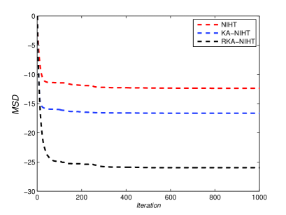
Fig. 1: The MSD versus iteration number, with $M=70$;

Fig. 2 (a) demonstrates the proportion of coefficients recovered in six methods with the dimension of the vector $\mathbf{y}$ varying from $M=40$ to $M=80$. Fig. 2 (b) shows the MSD performance.

We can conclude the following:

The proportion of correct recovery increases with the larger dimension of $\mathbf{y}$.

The recovery algorithms with prior information perform better than the original recovery algorithms such as the LW-OMP against OMP and KA-NIHT against NIHT.

As for the KA-NIHT and RKA-NIHT algorithms, the performance of the scheme with adjustable probabilities is better than that with fixed probabilities.

The RKA-NIHT algorithm shows a better performance than the LW-OMP algorithm, also exploiting the a priori probabilities.

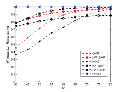
(a)

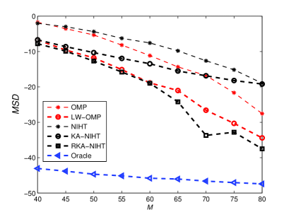
(b)

Fig. 2: The proportion of coefficients recovered and MSD versus sensing matrix dimension $M$.

Fig. 3 shows the algorithm performance for varying levels of noise. The length of $\mathbf{y}$ is $M=70$. Other parameters are the same as for Fig. 2. Results in Fig. 3 demonstrate that the proposed RKA-NIHT algorithm outperforms the other algorithms in the large range of the noise level.

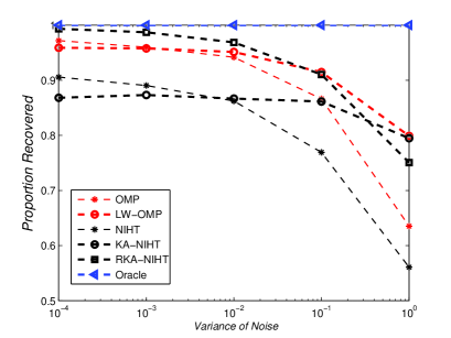
(a)

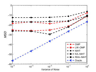
(b)

Fig. 3: The proportion of coefficients recovered and MSD versus variance of noise $\sigma^{2}$.

5 Conclusion

In this paper, we have developed knowledge-aided normalized iterative hard thresholding algorithms for sparse recovery problems. The proposed algorithms, named KA-NIHT and RKA-NIHT algorithms, have been designed considering the initial probabilities which are given at the start as prior knowledge and a recursive procedure to update the probabilities of the non-zero coefficients, respectively. The use of prior probabilities can improve the accuracy of finding the positions for non-zero elements. The simulations have shown that the proposed KA-NIHT and RKA-NIHT algorithms perform very well as compared to existing algorithms.

References

- [1] D. L. Donoho, “Compressed sensing,” IEEE Transactions on information theory, vol. 52, no. 4, pp. 1289–1306, 2006.
- [2] E. J. Candès and M. B. Wakin, “An introduction to compressive sampling,” IEEE signal processing magazine, vol. 25, no. 2, pp. 21–30, 2008.
- [3] R. C. de Lamare and R. Sampaio-Neto, “Adaptive reduced-rank mmse filtering with interpolated fir filters and adaptive interpolators,” IEEE Signal Processing Letters, vol. 12, no. 3, pp. 177–180, March 2005.
- [4] R. C. de Lamare and R. Sampaio-Neto, “Reduced-rank adaptive filtering based on joint iterative optimization of adaptive filters,” IEEE Signal Processing Letters, vol. 14, no. 12, pp. 980–983, Dec 2007.
- [5] R. C. de Lamare and R. Sampaio-Neto, “Adaptive reduced-rank processing based on joint and iterative interpolation, decimation, and filtering,” IEEE Transactions on Signal Processing, vol. 57, no. 7, pp. 2503–2514, July 2009.
- [6] R. C. de Lamare and P. S. R. Diniz, “Set-membership adaptive algorithms based on time-varying error bounds for cdma interference suppression,” IEEE Transactions on Vehicular Technology, vol. 58, no. 2, pp. 644–654, Feb 2009.
- [7] R. Fa, R. C. de Lamare, and L. Wang, “Reduced-rank stap schemes for airborne radar based on switched joint interpolation, decimation and filtering algorithm,” IEEE Transactions on Signal Processing, vol. 58, no. 8, pp. 4182–4194, Aug 2010.
- [8] Z. Yang, R. C. de Lamare, and X. Li, “-regularized stap algorithms with a generalized sidelobe canceler architecture for airborne radar,” IEEE Transactions on Signal Processing, vol. 60, no. 2, pp. 674–686, Feb 2012.
- [9] G. Li, X. Li, S. Li, H. Bai, Q. Jiang, and X. He, “Designing robust sensing matrix for image compression,” IEEE Transactions on Image Processing, vol. 24, no. 12, pp. 5389–5400, 2015.
- [10] S. Xu, R. C. de Lamare, and H. V. Poor, “Distributed compressed estimation based on compressive sensing,” IEEE Signal Processing Letters, vol. 22, no. 9, pp. 1311–1315, 2015.
- [11] J. Wright, A. Y. Yang, A. Ganesh, S. S. Sastry, and Y. Ma, “Robust face recognition via sparse representation,” IEEE transactions on pattern analysis and machine intelligence, vol. 31, no. 2, pp. 210–227, 2009.
- [12] Z. Zhu and M. B. Wakin, “Approximating sampled sinusoids and multiband signals using multiband modulated dpss dictionaries,” Journal of Fourier Analysis and Applications, pp. 1–48, 2016.
- [13] M. Aharon, M. Elad, and A. Bruckstein, “-svd: An algorithm for designing overcomplete dictionaries for sparse representation,” IEEE Transactions on signal processing, vol. 54, no. 11, pp. 4311–4322, 2006.
- [14] G. Li, Z. Zhu, D. Yang, L. Chang, and H. Bai, “On projection matrix optimization for compressive sensing systems,” IEEE Transactions on Signal Processing, vol. 61, no. 11, pp. 2887–2898, 2013.
- [15] Q. Jiang, S. Li, H. Bai, R. C. de Lamare, and X. He, “Gradient-based algorithm for designing sensing matrix considering real mutual coherence for compressed sensing systems,” IET Signal Processing, vol. 11, no. 4, pp. 356–363, 2017.
- [16] Y. C. Pati, R. Rezaiifar, and P. S. Krishnaprasad, “Orthogonal matching pursuit: Recursive function approximation with applications to wavelet decomposition,” in Proc. 27th Asilomar Conf. Signals Syst. Comput., 1993, pp. 40–44.
- [17] E. J. Candès and T. Tao, “Decoding by linear programming,” IEEE transactions on information theory, vol. 51, no. 12, pp. 4203–4215, 2005.
- [18] R. Tibshirani, “Regression shrinkage and selection via the lasso,” Journal of the Royal Statistical Society. Series B (Methodological), pp. 267–288, 1996.
- [19] T. Blumensath and M. E. Davies, “Iterative hard thresholding for compressed sensing,” Applied and computational harmonic analysis, vol. 27, no. 3, pp. 265–274, 2009.
- [20] Y. V. Zakharov, V. H. Nascimento, R. C. De Lamare, and F. G. D. A. Neto, “Low-complexity dcd-based sparse recovery algorithms,” IEEE Access, vol. 5, pp. 12737–12750, 2017.
- [21] R. C. de Lamare and R. Sampaio-Neto, “Sparsity-aware adaptive algorithms based on alternating optimization and shrinkage,” IEEE Signal Processing Letters, vol. 21, no. 2, pp. 225–229, Feb 2014.
- [22] M. Yukawa, R. C. de Lamare, and R. Sampaio-Neto, “Efficient acoustic echo cancellation with reduced-rank adaptive filtering based on selective decimation and adaptive interpolation,” IEEE Transactions on Audio, Speech, and Language Processing, vol. 16, no. 4, pp. 696–710, May 2008.
- [23] Y. Cai, R. C. de Lamare, B. Champagne, B. Qin, and M. Zhao, “Adaptive reduced-rank receive processing based on minimum symbol-error-rate criterion for large-scale multiple-antenna systems,” IEEE Transactions on Communications, vol. 63, no. 11, pp. 4185–4201, Nov 2015.
- [24] J. Liu and R. C. de Lamare, “Low-latency reweighted belief propagation decoding for ldpc codes,” IEEE Communications Letters, vol. 16, no. 10, pp. 1660–1663, October 2012.
- [25] Z. Yang, R. C. D. Lamare, and X. Li, “Sparsity-aware space-time adaptive processing algorithms with l1-norm regularisation for airborne radar,” IET Signal Processing, vol. 6, no. 5, pp. 413–423, July 2012.
- [26] R. C. De Lamare and R. Sampaio-Neto, “Minimum mean-squared error iterative successive parallel arbitrated decision feedback detectors for ds-cdma systems,” IEEE Transactions on Communications, vol. 56, no. 5, pp. 778–789, May 2008.
- [27] N. Song, W. U. Alokozai, R. C. de Lamare, and M. Haardt, “Adaptive widely linear reduced-rank beamforming based on joint iterative optimization,” IEEE Signal Processing Letters, vol. 21, no. 3, pp. 265–269, March 2014.
- [28] S. D. Somasundaram, N. H. Parsons, P. Li, and R. C. de Lamare, “Reduced-dimension robust capon beamforming using krylov-subspace techniques,” IEEE Transactions on Aerospace and Electronic Systems, vol. 51, no. 1, pp. 270–289, January 2015.
- [29] L. Wang, R. C. de Lamare, and M. Haardt, “Direction finding algorithms based on joint iterative subspace optimization,” IEEE Transactions on Aerospace and Electronic Systems, vol. 50, no. 4, pp. 2541–2553, October 2014.
- [30] L. Qiu, Y. Cai, R. C. de Lamare, and M. Zhao, “Reduced-rank doa estimation algorithms based on alternating low-rank decomposition,” IEEE Signal Processing Letters, vol. 23, no. 5, pp. 565–569, May 2016.
- [31] H. Ruan and R. C. de Lamare, “Robust adaptive beamforming using a low-complexity shrinkage-based mismatch estimation algorithm,” IEEE Signal Processing Letters, vol. 21, no. 1, pp. 60–64, Jan 2014.
- [32] H. Ruan and R. C. de Lamare, “Robust adaptive beamforming based on low-rank and cross-correlation techniques,” IEEE Transactions on Signal Processing, vol. 64, no. 15, pp. 3919–3932, Aug 2016.
- [33] R. C. de Lamare, “Adaptive and iterative multi-branch mmse decision feedback detection algorithms for multi-antenna systems,” IEEE Transactions on Wireless Communications, vol. 12, no. 10, pp. 5294–5308, October 2013.
- [34] W. Zhang, R. C. de Lamare, C. Pan, M. Chen, J. Dai, B. Wu, and X. Bao, “Widely linear precoding for large-scale mimo with iqi: Algorithms and performance analysis,” IEEE Transactions on Wireless Communications, vol. 16, no. 5, pp. 3298–3312, May 2017.
- [35] T. G. Miller, S. Xu, R. C. de Lamare, and H. V. Poor, “Distributed spectrum estimation based on alternating mixed discrete-continuous adaptation,” IEEE Signal Processing Letters, vol. 23, no. 4, pp. 551–555, April 2016.
- [36] J. Gu, R. C. de Lamare, and M. Huemer, “Buffer-aided physical-layer network coding with optimal linear code designs for cooperative networks,” IEEE Transactions on Communications, vol. 66, no. 6, pp. 2560–2575, June 2018.
- [37] S. F. B. Pinto and R. C. de Lamare, “Multi-step knowledge-aided iterative esprit: Design and analysis,” IEEE Transactions on Aerospace and Electronic Systems, pp. 1–1, 2018.
- [38] P. Clarke and R. C. de Lamare, “Transmit diversity and relay selection algorithms for multirelay cooperative mimo systems,” IEEE Transactions on Vehicular Technology, vol. 61, no. 3, pp. 1084–1098, March 2012.
- [39] M. F. Kaloorazi and R. C. de Lamare, “Subspace-orbit randomized decomposition for low-rank matrix approximations,” IEEE Transactions on Signal Processing, vol. 66, no. 16, pp. 4409–4424, Aug 2018.
- [40] D. L. Donoho and Y. Tsaig, “Fast solution of -norm minimization problems when the solution may be sparse,” IEEE Transactions on Information Theory, vol. 54, no. 11, pp. 4789–4812, 2008.
- [41] F. G. Almeida Neto, R. C. De Lamare, V. H. Nascimento, and Y. V. Zakharov, “Adaptive reweighting homotopy algorithms applied to beamforming,” IEEE Transactions on Aerospace and Electronic Systems, vol. 51, no. 3, pp. 1902–1915, July 2015.
- [42] C. J. Miosso, R. Borries, and J. H. Pierluissi, “Compressive sensing with prior information: Requirements and probabilities of reconstruction in -minimization,” IEEE Transactions on Signal Processing, vol. 61, no. 9, pp. 2150–2164, 2013.
- [43] J. F. C. Mota, N. Deligiannis, and M. R. D. Rodrigues, “Compressed sensing with prior information: Optimal strategies, geometry, and bounds,” arXiv preprint arXiv:1408.5250, 2014.
- [44] J. Scarlett, J. S Evans, and S. Dey, “Compressed sensing with prior information: Information-theoretic limits and practical decoders,” IEEE Transactions on Signal Processing, vol. 61, no. 2, pp. 427–439, 2013.
- [45] T. Blumensath and M. E. Davies, “Normalized iterative hard thresholding: Guaranteed stability and performance,” IEEE Journal of selected topics in signal processing, vol. 4, no. 2, pp. 298–309, 2010.
- [46] E. J. Candès, J. Romberg, and T. Tao, “Robust uncertainty principles: Exact signal reconstruction from highly incomplete frequency information,” IEEE Transactions on information theory, vol. 52, no. 2, pp. 489–509, 2006.