We present a novel approach to construct cosmological models endowed with a particular scalar field,
the stealth. The model is constructed by studying a scalar field no-minimally coupled to
the gravitational field with sources; as sources, we used a perfect fluid and analyzed the simplest
case of dust and the power-law cosmology. Surprisingly, we find that these stealth fields, which have
no back-reaction to background space-time, have a contribution to cosmological dynamics.
Furthermore, we provide analytic expressions of the stealth’s contributions to the energy density in
both cases, and for the pressure in the power-low cosmology, which means that such contributions
to cosmological evolution are quantifiable. Additionally, we discuss the behaviors of the
self-interaction potential for some cases.
Keywords:
First keyword Second keyword More
1 Introduction
The stealth fields are nontrivial solutions to scalar fields non-minimally coupled to the gravitational
field with a vanishing stress-energy tensor. This particular fact does not induce a back-reaction on
the background spacetime where the stealths propagate. The stealth fields based on the Einstein
field equations as well as in some modified gravity field equations have been fairly studied in the
last few years where their existence has been proved in several gravitational contexts
rubens ; poloco ; AyonBeato:2005tuA ; AyonBeato:2004ig ; banerj ; mokthar ; mokthar2 ; mokthar3 ; faraoni ; mokthar5 ; mokthar6 ; cisterna ; charmois ; temoc ; Smolic ; chilenos ; maeda ; Ayon-Beato:2013bsa ; Ayon-Beato:2015bsa .
In any case, despite the wealth of references quoted the
subject, from the field equations little can be concluded regarding the interaction between a stealth
field and ordinary matter. In this sense, we intend to develop further such subject in the present
work. In fact, remarkable results in this direction were provided in poloco where a deep
analysis of the interaction of matter which does not carry energy and the ordinary matter,
was performed.
One of the most outstanding conclusions from the current astronomical data has been the
confirmation of the late cosmic acceleration of the Universe SnIa . Until now, the best fit to
this data is by using the well known Cold Dark Matter (CDM) model. This
model necessarily includes a cosmological constant to make it work and exhibit an accelerated
behavior of the Universe but the criticism is that such constant is included by hand into the
model. This fact leaves several questions and concerns, mainly about the nature of the constant;
for example, its origin and value that are very close to critical energy density confronting thus the
predictions made by the quantum field theory in approximately 120 orders of magnitude. There
are two main approaches pursued to describe the phenomenon of the cosmic acceleration: the
first one is based in the inclusion of an exotic matter, i.e. the dark energy (DE) where the
cosmological constant drives the expansion; the second one, by modifying the Einstein gravity
theory where some non-standard geometrical terms lead to an accelerated performance. While
these models are interesting, it is probably fair to say that their results about the accelerated
behavior of the Universe are not conclusive, especially when they are compared to those
from CDM model.
On the other hand, the stealth fields in the cosmological context have been a focus of great interest
since the so-called dark energy sector of the Universe seems to be a special arena where modified
gravity theories, and observations, may be contrasted. In this spirit, in 1972 was shown that
the presence of a stealth field in a cosmological scenario is able to reproduce the observational data.
In view of this situation, encouraged by their particular behaviors as well the possibility to grasp
their role into the cosmological setup, one may wonder if the stealth field evolution in a
Friedmann-Lemaître- Robertson-Walker (FLRW) spacetime coupled to a perfect fluid indicates
a viable alternative to explain the accelerated expansion of the universe. There are other approaches
that pursue the same goal such as quintessence shani , Chaplygin gas chaplin and its
generalization chaplinG , -essence kessence , to mention something. In all these
cases, they invoke a scalar field to drive the cosmic acceleration. Following this line of reasoning,
in this paper, we construct a cosmological model endowed with a scalar field, the stealth field,
with the particular fact that it does not back-react on an FLRW background spacetime, contrary to
the above mentioned models. As a result, we obtain a general approach relating the stealth with
any type of matter coupled to the gravitational field.
In this work, we attempt to carry one step further the FLRW geometry as a background spacetime
where the stealth field propagate, endowing it with matter content provided by dust. By
respecting the vanishing of the stress tensor associated to the stealth as field equations, we
explicitly construct solutions for as well as the self-interacting potential. At dependence of
the parameters of the theory, this may (or not) have some non-trivial impacts on the cosmology
of the Universe.
The paper is organized as follows. In section 2 the general approach for the stealth in presence of
sources is given. In section 3 we used the approach to study the stealth in the presence of dust.
In section 4 an example of the stealth in a power law universe expansion is studied, finally, in
section 5 we end with a discussion and conclusions are given.
2 Stealths in presence of sources
The stealth fields are characteristics of Hordensky theories of gravitation where the
scalar fields are coupled non-minimally to gravity. In the present work, we study the stealth in an
FLRW space-time with a perfect fluid and its cosmological consequences. An action describing such
a scenario is,
(1)
In the above expression, is the coupling constant, is the matter
Lagrangian, is the scalar field, and is the self-interaction potential of the scalar field.
The field equations obtained from the variation of the action (1) with respect to the
metric are written as
(2)
where is the stress-energy tensor of ordinary matter and
is the stress-energy tensor of the stealth field
; explicitly:
(3)
Meanwhile, from variation with respect to the scalar field, the equation which describes its dynamics
is obtained
(4)
The existence of a stealth field for a given background is established by the vanishing of (2);
(5)
and its solutions and must satisfy the equation which describes the dynamics of
scalar field,
(6)
obtained by the variation of (1) with respect to the scalar field. At this point, the problem
is to solve the system of equations (5) and (6).
However, as was pointed out in mokthar the fulfillment of Eq.(6) is warranted from
the conservation of the energy-momentum stealth tensor due to diffeomorphism invariance of the
action (1),
(7)
which means that solutions of (5) satisfying (7) are necessarily solutions of
(6).
In the present work, for the construction of the stress-energy tensor for the stealth field
, we give the matter information of the Einstein’s equations instead of the
geometrical one, so then the ordinary matter it is related with the stealth field through the
expression,
(8)
It is remarkable that this expression is consistent just only when stealth configurations exist.
In what follows, we will consider that scalar field is homogeneous, i.e. depend only on time.
3 Stealth’s cosmological models
Bearing in mind the picture of the Universe by the Big Bang theory, we will model it with a perfect
fluid in an FLRW background.
(9)
as usual, the scale factor is a function of time.
As a source we use a perfect fluid stress-energy tensor
, where is the pressure,
the energy density and is the -velocity of the fluid with
. By substituting this tensor into (8) we obtain;
(10)
(11)
where ; there are two independent equations, one from the spatial component and
the other from the time component.
The cosmological model is realized combining Eq.(11) and using the fact
that the density in that equation must correspond with the given by GR, then it
must satisfied the Friedmann equation , so
(12)
The simplest case to study is the dust case, that is, . So from (10) for the
self-interacting potential we get
Now the problem has been reduced to finding the stealth field , while the energy
density and the potential are given by the above equations.
In the dust case, the non-relativistic matter contribution behaves as
. Then, we try to integrate Eq. (14) using the density
, however, the direct substitution of the in
(14) leads us to a Riccati equation and for this case, there is no analytic
solution. We are interested in the analytic solutions of Eq. (14);
therefore, we propose to seek solutions for that depends only on the scale
factor, i.e., , so Eq. (14) turns out to be
(15)
where we have defined , (for more detail see appendix 7). It is worth to remark
that the solutions to the above equation have different behaviors depending on the range of possible
values of , as we will see below.
3.1 Homogeneous cosmologies for
By integrating (15), we obtain for the scalar field
(16)
where
here and are integration constants.
Now, for the same range of values for , the potential is obtained by substitution of
the above equation into (13),
(17)
where we have defined and
. It is verify by substitution
of (16) into (14) the right expression to the density .
At this point, we have obtained a stealth model that mimics exactly a matter dominated universe. It is
important to remark that has to be positive and this would eventually implies a new range for
the coupling .
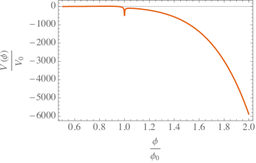
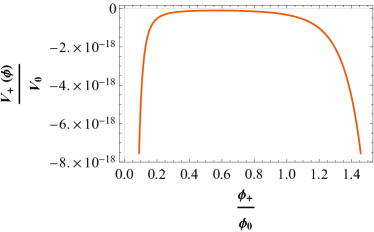
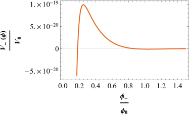
In the following figure we show the graphs of vs. , for four
different values of the parameters in .
Figure 1: The left panel shows vs.
for the values , , , , and ; and
at the right panel for , , , , and .
As is clear from Fig.(1) the potential is nearly flat near and positive as the values
of increase. The same happens for both cases, although the left panel shows a sharp deep well
around . It is interesting to note that for values of , the discriminant of the root
in always become positive so for this case the solutions given by Eq. (16) remain
valid. From the analysis of this solution shows that stealths can appear at the same time as spacetime,
as we will see later it is not obvious, some solutions allow stealths sometime after the cosmological
evolution begun.
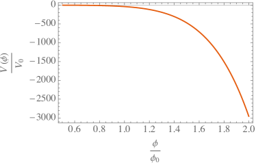
Figure 2: The left panel takes the values , , , , and
; and the right panel , , ,
, and .
In Fig.(2) it is shown the case where . The left panel shows a nearly flat
potential in the entire range of with a similar sharp deep well around as we see in
the previous case. The right panel is completely different compared to the previous cases. It is positive
and decaying in all the range of the scalar field, and diverges at the origin .
The term in Eq.(16) will appear constantly from here on in the solution for
stealth and there is no reason to constrain its value, so it could be positive,
imaginary or null, depending if its value becomes greater than, less than or equal
to . Now the solution (16) remain valid to the ranges
. The critical value
, the range and will be analyzed in
separate subsections. It is interesting to note that for values of , the
discriminant of the root in always become positive so for this case the
solution given by Eq. (16) remain valid.
3.2 Stealth cosmology for
As was pointed out in the previous section, the value for is not
described by (16). In order to get the solution for this value we
substitute directly on (15), so we have
(18)
and the potential associated to the above equation becomes
(19)
where we have defined , and . Once again was verified the right functional form of by substituting
(18) into (14).
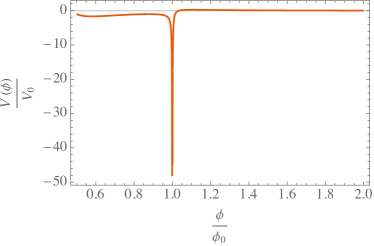
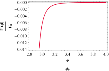
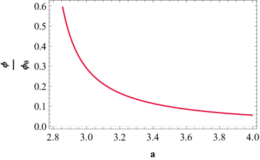
In the figure (3) we show the potential to different values of the
parameters, as one can see we do not include the graph for because it shows a
similar as the first graph.
Figure 3: At the left we show the self-interaction potential vs.
the scalar field and the graph on the right is for the scalar field vs. is the scale factor. The
values used are , , , ,
, and .
An interesting fact that emerges from the analysis of this solution is that the field only reaches
real values after a certain time of evolution of the scale factor. So, in this case, the stealth appears
after of space-time, and the values of and make the graph start closer or farther
from the origin.
3.3 Stealth cosmology for
From (3) in the range the discriminant of
is negative, the exponent is complex, so that we have oscillating solutions given by
(20)
where and are constants. Now, if we define the constants as
and , we can get a simpler scalar field, this is
(21)
and its potential
(22)
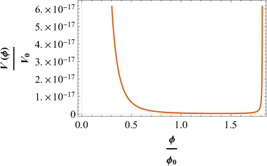
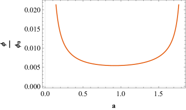
The graph for this case is shown in figure (4), the stealth field, in this case, have a periods
of real and complex values, which are longer as the value of the phase into the cosine increase.
Figure 4: At the left we show the self-interaction potential vs.
the scalar field and
the graph on the right is for the scalar field vs. is the scale factor. The values used are
, , , , and .
3.4 Stealth cosmologies for
There is a special case for .
In particular here it is possible to integrate the general case. Under the change
Eq. (15) is written as
(23)
Now from the above equation it is evident why this value for is a special
value, and in general its integral is
(24)
and its self-interaction potential gives
(25)
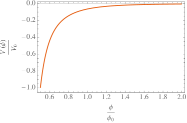
The behavior for both potentials is displayed in Fig.(5).
Figure 5: At the left we show the self-interaction of the scalar field
vs.
for the values , , , , and ;
While at the right we show vs.
for the values , , , , and .
In the figures of this section we wish study the sensibility of the potential to
the sign of the integration constants. For this case the solution allow stealth at same time as the start
of spacetime.
4 Homogeneous power law cosmologies
In this section, we show the advantages of our approach by studying the contributions of the stealth
field to the principal quantities setting up the cosmology from the Einstein equations, that is, the
energy density and the pressure. In order to prove our approach, we reproduce some of the results
reported in Ayon-Beato:2015bsa , we study the power law for homogeneous
cosmologies. As in previous case, the behavior of stealth
depends on value of so we study the solutions for the more general cases
reported in the work aforementioned. Even more, in what follows we use the
conformal metric as in Ayon-Beato:2015bsa ,
(26)
In this case from Eq. (8), we get the expressions for and
(27)
(28)
Adding (27) and (28) and doing the same for the expressions of and
obtained from field equations of GR, we obtain the equations for the stealth field and its
self-interaction potential ,
(29)
now subtracting Eqs. (27) and (28) and by using again and from GR,
(30)
By substituting (30) into Eqs. (27) and (28), we get
(31)
(32)
From the above equations, it is clear that is possible to quantify the contributions to the stealth field
to and . In order to realize the cosmology the Friedmann equation in the spacetime
described by (26) is with state equation
, explicitly for Friedmann equation in terms of stealth
(33)
and for power-law cosmologies, the state equation remains valid.
4.1 Homogeneous cosmologies with
As in the previous section, the behavior of the solution of (29) for depends on the value
of so we study the solutions in its different regimes or ranges.
(34)
A contribution of our work to the solutions found in Ayon-Beato:2015bsa are the expressions
for the energy density and pressure given by the Eqs. (27) and (28), respectively,
(35)
(36)
(37)
It is worth mentioning that all terms in the above expressions which depend explicitly on time are
contributions of the stealth field. The term vanish with the contribution of
.
4.2 Homogeneous cosmologies for
At the value of Eq.(34) fail so this case must be
integrated in separate way. Substituting this value into Eq.(29) the stealth
field
(38)
here and , are integration constants.
For this ranges the energy-density and the pressure are given by
(39)
(40)
where we have defined .
4.3 Homogeneous cosmologies for
There is a range for and where the discriminant of the solution becomes to be negative;
for this range the solutions are oscillating. At a difference of the reported in
Ayon-Beato:2015bsa , we do not use the relic symmetries approach. So we present directly the
solution of (29) and shown the expressions for and . In both cases our approach
work.
(41)
, are integration constants.
Now the energy density and the pressure are
(42)
(43)
we have defined ,
note that vanish linear contributions in as in first case, and it is
necessary to recovery the behavior of and .
Finally we recover the state equation since all the contributions
to density energy and pressure are which are the predict
behavior of GR, at difference in this theory, we quantify the contributions from
stealth field.
We decided don’t include the potentials for all the cases reviewed here cause has
been studied very well in Ayon-Beato:2015bsa , and the purpose of this
work it is to shown the quantify relations of stealth contributions to the
cosmology.
5 Conclusions
The main goal of this work is to provide a novel approach to construct cosmological models endowed
with stealth. We studied the stealth configurations in presence of sources, choosing a perfect fluid
and particularizing it to study two cases, dust, and the power law, both in a homogeneous
cosmology. As a result, we obtain a general approach to relate the stealth with any kind of matter
coupled to the gravitational field whenever there is stealth on it. As the stealths are such that they do
not warp the background spacetime, intuitively expected to play a role in the cosmological dynamics.
In this sense, there was provided a way to be quantified their contributions, namely, through
expressions for energy density and the pressure. This was achieved by giving the matter information
to the system of equations which gives room to a stealth field configuration instead of the geometrical.
For completeness, we show the behavior of some cases of the self-interaction potential for the
stealth, focusing on the sensibility of the sign of the integration constants. The reason for this last
issue because we expect that the parameter be fixed when the model will be contrasted
against observational data as was shown in 1972 . From the analysis of the solutions, the
stealth is allowed from the beginning of spacetime, except when where its
existence starting after the beginning of spacetime.
In future works, we will use the approach to study subclasses of the Hordensky’s theories which
have self-tuning mechanism, for example, those reported in 4fabs . Additionally, we explore
the perturbations like in odinstov , where some clues that what could happen with our
proposal.
6 Acknowledgments
Authors thank to Eloy Ayón-Beato for enlightening discussions.
Special thanks to Carlos Manuel Rodríguez.
CC acknowledges partial support by CONACyT Grant CB-2012-177519-F
and grant PROMEP, CA-UV, Álgebra, Geometría y
Gravitación. This work was partially supported by SNI (México).
VHC acknowledges partial support by DIUV-REG-50/2013.
AA acknowledges partial support by CONACyT Grant Estancias Posdoctorales
Vinculadas al Fortalecimiento de Calidad del Posgrado Nacional 2016.
7 Appendix A: Stealth field equation
We study the consequences of the stealth in cosmology,
Einstein’s field equations for a perfect fluid source are furnished by
(44)
here is are the Einstein tensor, is the energy momentum tensor of a
perfect fluid
(45)
where is the pressure, the energy density, is the fluid velocity four
vector with . is the stress energy tensor of the stealth
field (3).
The Friedmann-Lemaitre-Robertson-Walker metric for a homogeneous isotropic universe is provided
by
(46)
where , indicating the spatial curvature constants. In the case the field equations
for the background
are given by
(47)
(48)
and the continuity equation that satisfies the fluid is
(49)
Now, we assume that the universe is spatially flat and the dust case, i.e. when the pressure is zero.
We go back to the equations (47) and (49), to obtain that density and scale factor
are given explicitly in the form
(50)
(51)
in thats case the equations for the stealth are given by the Eq.(14).
factorizing and rearranging terms and by
substituting the expressions of and one arrive at Eq.(15).
References
(1)
R. Cordero and A. Vilenkin,
Phys. Rev. D 65, 083519 (2002) [hep-th/0107175].
(2)
L. M. Sokolowski,
Acta Phys. Polon. B 35, 587 (2004)
[gr-qc/0310113].
(3)
E. Ayón-Beato, C. Martínez, R. Troncoso and J. Zanelli,
Phys. Rev. D 71, 104037 (2005)
[hep-th/0505086].
(4)
E. Ayón-Beato, C. Martínez and J. Zanelli,
Gen. Rel. Grav. 38, 145 (2006)
[hep-th/0403228].
(5)
N. Banerjee, R. K. Jain and D. P. Jatkar,
Gen. Rel. Grav. 40, 93 (2008 [hep-th/0610109].
(6)
E. Ayón-Beato, M. Hassaïne and M. M. Juárez-Aubry,
arXiv:1506.03545 [gr-qc].
(7)
M. M. Caldarelli, C. Charmousis and M. Hassaïne,
JHEP 1310, 015 (2013)
[arXiv:1307.5063 [hep-th]].
(8)
M. Bravo-Gaete and M. Hassaïne,
Phys. Rev. D 88, 104011 (2013)
[arXiv:1308.3076 [hep-th]].
(9)
V. Faraoni, A. F. Zambrano-Moreno, Phys. Rev. D 81 124050 (2010). arxiv:1006.1936 [gr-qc]
(10)
M. Hassaïne,
Phys. Rev. D 89, no. 4, 044009 (2014)
[arXiv:1311.4623 [hep-th]].
(11)
M. Bravo-Gaete and M. Hassaïne,
Phys. Rev. D 90, no. 2, 024008 (2014)
[arXiv:1405.4935 [hep-th]].
(12)
A. Cisterna, M. Hassaïne, J. Oliva and M. Rinaldi,
Phys. Rev. D 94, no. 10, 104039 (2016)
[arXiv:1609.03430 [gr-qc]].
(13)
E. Babichev, C. Charmousis and M. Hassaïne,
JCAP 1505, 031 (2015)
[arXiv:1503.02545 [gr-qc]].
(14)
A. Alvarez, C. Campuzano, M. Cruz, E. Rojas and J. Saavedra,
Gen. Rel. Grav. 48, no. 12, 165 (2016)
[arXiv:1611.03022 [gr-qc]].
(15)
I. Smolic̀, Phys. Rev. D 97, no.8, 084041 (2018). [arxiv.org:1711.07490][gr-qc]
(16)
C. Quinzacara, P. Meza, A. Sampson and M. Valenzuela. [arxiv.org:1805.04621][hep-th] (2018).
(17)
H. Maeda and K. i. Maeda,
Phys. Rev. D 86, 124045 (2012)
[arXiv:1208.5777 [gr-qc]].
(18)
E. Ayón-Beato, A. A. García, P. I. Ramírez-Baca and C. A. Terrero-Escalante,
Phys. Rev. D 88, no. 6, 063523 (2013)
[arXiv:1307.6534 [gr-qc]].
(19)
E. Ayón-Beato, P. I. Ramírez-Baca and C. A. Terrero-Escalante,
Phys. Rev. D 97, no. 4, 043505 (2018)
[arXiv:1512.09375 [gr-qc]]. (2015).
(20)
S. Perlmutter, et. al. ApJ, 517, 565 (1999); A. G. Ries et. al. AJ, 116, 1009 (1998);
B. P. Schmidt, ApJ, 507, 46 (1998).
(21)
C. Campuzano, V. H. Cárdenas and R. Herrera,
Eur. Phys. J. C 76, no. 12, 698 (2016)
[arXiv:1611.08433 [gr-qc]].
(22)
C. Wetterich, Nucl. Phys. B 302, 668 (1988);
B. Ratra, P.J.E. Peebles, Phys. Rev. D 37, 3406 (1988);
J.A. Frieman, C.T. Hill, A. Stebbins, I. Waga, Phys. Rev. Lett. 75, 2077 (1995);
M.S. Turner, M. White, Phys. Rev. D 56, R4439 (1997);
R.R. Caldwell, R. Dave, P.J. Steinhardt, Phys. Rev. Lett. 76, 1582 (1998);
P.J. Steinhardt, L.Wang, I. Zlatev, Phys. Rev. D 59, 123504 (1999);
V. Sahni and L. M. Wang,
Phys. Rev. D 62, 103517 (2000).
[astro-ph/9910097].
(23)
A. Y. Kamenshchik, U. Moschella and V. Pasquier,
Phys. Lett. B 511, 265 (2001)
[gr-qc/0103004].
(24)
M. C. Bento, O. Bertolami and A. A. Sen,
Phys. Rev. D 66, 043507 (2002)
[gr-qc/0202064].
(25)
R. J. Scherrer,
Phys. Rev. Lett. 93, 011301 (2004)
[astro-ph/0402316].
(26)
C. Charmousis, J. Edmund, E. J. Copeland, A. Padilla, P. M. Saffin,
Phys. Rev. Lett. 108 051101 (2012). arxiv: 1106.2000 [hep-th]
(27)
A. V. Astashenok and S. D. Odintsov, Phys. Lett. B, 718, 1194 (2013).