Using non-solar-scaled opacities to derive stellar parameters

Abstract

Aims. In an effort trying to improve spectroscopic methods of stellar parameters determination, we implemented non-solar-scaled opacities in a simultaneous derivation of fundamental parameters and abundances. We want to compare the results with the usual solar-scaled method using a sample of solar-type and evolved stars.

Methods. We carried out a high-precision stellar parameters and abundance determination by applying non-solar-scaled opacities and model atmospheres. Our sample is composed by 20 stars (including main-sequence and evolved objects), with six stars belonging to binary systems. The stellar parameters were determined by imposing ionization and excitation equilibrium of Fe lines, with an updated version of the FUNDPAR program, together with plane-parallel ATLAS12 model atmospheres and the MOOG code. Opacities for an arbitrary composition and v_micro were calculated through the OS (Opacity Sampling) method. Detailed abundances were derived using equivalent widths and spectral synthesis with the MOOG program. We applied the full line-by-line differential technique using the Sun as reference star, both in the derivation of stellar parameters and in the abundance determination. We start using solar-scaled models in a first step, and then continue the process but scaling to the abundance values found in the previous step (i.e. non-solar-scaled). The process finish when the stellar parameters of one step are the same of the previous step, i.e. we use a doubly-iterated method.

Results. We obtained a small difference in stellar parameters derived with non-solar-scaled opacities compared to classical solar-scaled models. The differences in T_eff, log g and [Fe/H] amount up to 26 K, 0.05 dex and 0.020 dex for the stars in our sample. These differences could be considered as the first estimation of the error due to the use of classical solar-scaled opacities to derive stellar parameters with solar-type and evolved stars. We note that some chemical species could also show an individual variation higher than those of the [Fe/H] (up to $\sim$0.03 dex) and varying from one specie to another, obtaining a chemical pattern difference between both methods. This means that condensation temperature T_c trends could also present a variation. We include an example showing that using non-solar-scaled opacities, the solution found with the classical solar-scaled method indeed cannot always verify the excitation and ionization balance conditions required for a model atmosphere. We discuss in the text the significance of the differences obtained when using solar-scaled vs non-solar-scaled methods.

Conclusions. We consider that the use of the non-solar-scaled opacities is not mandatory e.g. in every statistical study with large samples of stars. However, for those high-precision works whose results depend on the mutual comparison of different chemical species (such as the analysis of condensation temperature T_c trends), we consider that it is whortwhile its aplication. To date, this is probably one of the more precise spectroscopic methods of stellar parameters derivation.

1 Introduction

The discovery of the first exoplanets orbiting the pulsar PSR1257+12 (Wolszczan & Frail, 1992) and the solar-type star 51 Peg (Mayor & Queloz, 1995), gave rise to a number of works which strongly motivated to increase the precision of both photometry and spectroscopy techniques. This continuous effort allowed the discovery of new planets and its subsequent analysis. For instance, radial-velocity measurements improved to a precision of few m/s or less (e.g. Lo Curto et al., 2015; Fischer et al., 2016), while the Kepler photometry could reach ¡ 1 millimag for a 12^th mag star. The derivation of detailed chemical abundances followed a similar path. For example, the use of the called differential technique applied to physically similar stars, allowed to significantly reduce the dispersion in [Fe/H] to values near or lower than $\sim$0.01 dex (e.g. Desidera et al., 2004; Meléndez et al., 2009; Ramírez et al., 2011; Saffe et al., 2015, 2016, 2017). These high precision values are needed, for example, to detect a possible chemical signature of planet formation (e.g. Meléndez et al., 2009; Saffe et al., 2016) and also required by the chemical tagging technique. Then, it is crucial to pursuit the maximum possible precision in the derivation of stellar parameters and chemical patterns.

Several works studying the chemical composition of solar-type stars use a two-step method of abundance determination. For instance, in the study of stellar galactic populations (e.g. Adibekyan et al., 2012, 2013, 2014, 2016; Delgado Mena et al., 2017), metallicity trends in stars with and without planets (e.g. Sousa et al., 2008, 2011a, 2011b; Adibekyan et al., 2012), and the possible signature of terrestrial planets (e.g. González Hernández et al., 2010, 2013; Adibekyan et al., 2014). These works are not an exhaustive list but exemplify a number of important studies and trends. Briefly, in a first step the fundamental parameters are determined by imposing excitation and ionization equilibrium of Fe I and Fe II lines. The model atmosphere which satisfy these conditions is usually interpolated or calculated by assuming both solar-scaled opacities and abundances. Once fixed the stellar parameters, in a second step the chemical abundances are determined by using equivalent widths or spectral synthesis, depending on the possible presence of blends and other effects such as hyperfine structure (HFS). The process normally finishes here, resulting in a chemical pattern that is not exactly solar-scaled, as supposed in the first step. Notably, even reaching a perfect match between synthetic and observed spectra, this inconsistency could lead to an incorrect determination of stellar parameters and abundances. In addition, this issue is generally unaccounted in the total error estimation of most literature works.

Then, in an effort to improve the precision of the results, the approppriate calculation of the model atmospheres should include the previous derivation of opacities obtained for a specific abundance pattern, beyond the classical solar-scaled values. We wonder if it is possible to implement such method in the calculation of stellar parameters in a practical way. What is the difference in the stellar parameters obtained with this procedure and the classical solar-scaled methods? How many iteration steps are neccessary to properly derive the stellar parameters? Can this effect introduce a statistical bias in studies of large samples? Do we expect a null difference in metallicity between very similar components of binary stars? These important questions are the motivation of the present work.

This work is organized as follows. In Sect. 2 we describe the sample and data reduction, while in Sect. 3 we explain the calculation of opacities and models. Finally, we present the discussion and conclusions in Sect. 4 and 5.

2 Sample of spectra

As previously mentioned, the detection of the possible chemical signature of planet formation requires a very high precision in stellar parameters. These studies are usually performed on solar-type main-sequence stars (e.g. Tucci Maia et al., 2014; Saffe et al., 2015, 2016). We start by choosing 10 objects of this type for our sample. In order to study the possible differences between solar-scaled and non-solar-scaled methods in other type of stars, we also included in our sample 10 giants stars (see Table 1). Then, the final sample is composed by 20 stars with T_eff in the range 4131-8333 K and log g in the range 1.62-4.64 dex. Their metallicities range from $-$0.43 to $+$0.27 dex i.e. including objects with values lower and higher than the Sun, and likely including a number of different chemical mixtures. Six stars in our sample belong to binary systems previously studied in the literature (Saffe et al., 2015, 2016, 2017, hereafter SA15, SA16, SA17). In particular, the binary systems were selected due to a high degree of physical similarity between their components, which allow to test the possible variation of the stellar parameters (scaled vs non-solar-scaled methods) depending on the chemical pattern, which is roughly similar for the two stars in each binary system.

For the stars studied in this work, Table 1 presents the corresponding spectrograph, resolving power, signal to noise and object used as a proxy for the Sun spectra. We reduced the data by using the reduction package MAKEE 3 with HIRES spectra, the DRS pipeline (Data Reduction Software) with HARPS data and the OPERA 5 (Martioli et al., 2012) software with GRACES spectra. The continuum normalization and other operations (such as Doppler correction and combining spectra) were perfomed using Image Reduction and Analysis Facility (IRAF).

Table 1: Sample of spectra used in this work.

Stars	Spectrograph	R	S/N	Sun
				spectra
Main-sequence stars
HD 80606 + HD 80607	HIRES	67000	$\sim$330	Iris
$\zeta^{1}$ Ret + $\zeta^{2}$ Ret	HARPS	110000	$\sim$300	Ganymede
HAT-P-4 + TYC 2567-744-1	GRACES	67500	$\sim$400	Moon
HD 19994	HARPS	115000	$\sim$390	Ganymede
HD 221287	HARPS	115000	$\sim$130	Ganymede
HD 96568	HARPS	115000	$\sim$350	Ganymede
HD 128898	HARPS	115000	$\sim$340	Ganymede
Evolved stars
HD 2114	HARPS	115000	$\sim$180	Ganymede
HD 10761	HARPS	115000	$\sim$195	Ganymede
HD 28305	HARPS	115000	$\sim$180	Ganymede
HD 32887	HARPS	115000	$\sim$245	Ganymede
HD 43023	HARPS	115000	$\sim$275	Ganymede
HD 50778	HARPS	115000	$\sim$140	Ganymede
HD 85444	HARPS	115000	$\sim$225	Ganymede
HD 109379	HARPS	115000	$\sim$335	Ganymede
HD 115659	HARPS	115000	$\sim$310	Ganymede
HD 152334	HARPS	115000	$\sim$195	Ganymede

3 Calculating non-solar-scaled opacities and models

Within the suite of Kurucz’s programs for model atmosphere calculation, a non-solar-scaled model can be calculated mainly in two different ways. The first option consists in the previous calculation of an Opacity Distribution Function (ODF) which depends on the abundances and microturbulence velocity v_micro, which is then used as input for an ATLAS9 model atmosphere (see e.g. Kurucz et al., 1974; Castelli, 2005b). The second option consists directly in the calculation of an ATLAS12 model atmosphere, which calculates internally the opacities through the Opacity Sampling (OS) method (see e.g. Peytremann, 1974; Kurucz, 1992; Castelli, 2005a).

We will briefly describe both options here. ODF functions used by ATLAS9 are tables which describe the dependence of the line absorption coefficient l_ν as a function of the frequency $\nu$, calculated for a given pair T_gas and P_gas (see e.g. Kurucz et al., 1974; Castelli, 2005b). Different sets of ODFs are derived for fixed abundances (usually solar-scaled and some $\alpha$-enhanced models) and fixed v_micro (see e.g. Castelli & Kurucz, 2003; Coelho, 2014). Strictly speaking, the calculation of an ATLAS9 model atmosphere for an specific composition and v_micro should include the previous calculation of the ODF for the corresponding values using the DFSYNTHE program (see e.g. Castelli, 2005b). Otherwise, the numerical abundances derived for the ions during the actual model calculation at a given gas state (T_gas and P_gas) will differ from the ones calculated during the ODF computation. On the other hand, it is also possible to derive an ATLAS12 model atmosphere in which the OS method determines the opacity for given abundances and v_micro. This is an important detail, given that the correct derivation of a model atmosphere for an arbitrary chemical pattern should include the specific opacities, and not only a mere change in the abundances used. The longer time required by the calculation of an ATLAS12 model compared to ATLAS9 is not a problem today, finishing the operation after only few minutes. There is available a complete ATLAS12 version for gfortran at the Fiorella Castelli’s webpage, while for DFSYNTHE there is only an ifort (intel) version. Then, we use ATLAS12 for the calculation of a non-solar-scaled model atmosphere.

Usually, ATLAS12 model atmospheres are used when the chemical composition of the stars present e.g. alpha-elements patterns that do not follow solar-scaled or alpha-enhanced models, or early-type stars where diffussion effects change significatively their superficial composition (see e.g. Sbordone et al., 2005; Mucciarelli et al., 2012). In this work, we use non-solar-scaled opacities (calculated by ATLAS12) for the simultaneous derivation of both stellar parameters and abundances, as we explain in the next Section.

4 Stellar parameters and chemical abundance analysis

We started by measuring the equivalent widths of Fe I and Fe II lines in the spectra using the IRAF task splot, and then continued with other chemical species. The lines list and relevant laboratory data (such as excitation potential and oscilator strengths) are similar to those used in previous works (SA15, SA16). However we note that the exact values are not very relevant here, given the differential technique applied in this case.

The first estimation of the stellar parameters (T_eff, log g, [Fe/H], v_micro) uses an iterative process within the FUNDPAR program (Saffe, 2011), searching for a model atmosphere which satisfies the excitation and ionization balance of Fe I and Fe II lines. This code was improved in order to use the program MOOG (Sneden, 1973) together with ATLAS12 opacities and model atmospheres (Kurucz, 1993). The procedure uses explicitly calculated (i.e. non-interpolated) plane-parallel local thermodynamic equilibrium (LTE) Kurucz’s model atmospheres with ATLAS12, which includes the internal calculation of the line opacities through the Opacity Sampling (OS) method. Two runs of ATLAS12 are used (see e.g. Castelli, 2005a): the first one for a preselection of important lines (for the given stellar parameters and abundances) and the second for the final calculation of the model structure. In both runs we explicitly use a specific chemical pattern.

The models are calculated with overshooting in order to facilitate the comparison with previous works (e.g. Saffe et al., 2015, 2016, 2017). However, we caution that this modification of the mixing-length theory is suitable for the Sun but not neccesarily for other stars (Castelli et al., 1997). The overshooting produces a thermal structure that disagrees with that obtained from hydrodynamical simulations, being magnified for low metallicity and dissapears for solar metallicity (see Fig. C.1 in Bonifacio et al., 2009). We adopted the layer 36 in the atmosphere where numerical results related with the Schwarzschild criterion can be assumed as reliable for models with T_eff $>$ 4000 K (Castelli, 2005a).

We applied in this work the full differential technique i.e. we consider the individual line-by-line differences between each star and the Sun, which is used as the reference star. The object used as a proxy for the solar spectra (in reflected light) is listed in the last column of Table 1. First, we determined absolute abundances for the Sun using 5777 K for T_eff, 4.44 dex for log g and an initial v_micro of 1.0 km/s. Then, we estimated v_micro for the Sun with the usual method of requiring zero slope in the absolute abundances of Fe I lines vs. reduced equivalent widths and obtained a final v_micro of 0.91 km/s. We note, however, that the exact values are not crucial for our strictly differential study (see e.g. Bedell et al., 2014; Saffe et al., 2015). The next step is the derivation of stellar parameters for all stars in our sample using the Sun as reference i.e. (star - Sun). We want to stress that this line-by-line method is applied both in the derivation of stellar parameters and in the chemical abundances (i.e. the ”full” differential technique), allowing to increase the precision of stellar parameters (e.g. Saffe et al., 2015, 2016).

In the first FUNDPAR iteration we use solar-scaled models for an initial estimation of stellar parameters. Then, a starting set of chemical abundances are determined using equivalent widths and spectral synthesis. In the next step, the iterative process within FUNDPAR is restarted but scaling using the last set of abundances instead of the initial solar-scaled values. At this point, we take advantage of the ATLAS12 opacities and models calculated ”on the fly” at the request of FUNDPAR, for an arbitrary chemical composition and v_micro. We note that the possibility to scale to an arbitrary chemical pattern (through an ABUNDANCE SCALE control card) was implemented by Dr. Fiorella Castelli and is not available in the original Kurucz code (Castelli, 2005a). In this way, new stellar parameters and abundances are succesively derived, finishing the process consistently when the stellar parameters are the same of the previous step. The process described here is then a doubly-iterated process, with the FUNDPAR iteration contained within a larger (abundance-scaled) iteration. The classical solar-scaled results correspond to the values derived in the first step of this new scheme.

We computed the individual abundances for the following elements: C I, O I, Na I, Mg I, Al I, Si I, S I, Ca I, Sc I, Sc II, Ti I, Ti II, V I, Cr I, Cr II, Mn I, Fe I, Fe II, Co I, Ni I, Cu I, Sr I, Y II, and Ba II. The HFS splitting was considered for V I, Mn I, Co I, Cu I and Ba II, by adopting the HFS constants of Kurucz & Bell (1995) and performing spectral synthesis with the program MOOG (Sneden, 1973) for these species. We used exactly the same lines (laboratory data and equivalent widths) for iron and for all chemical species, when deriving stellar parameters and abundances with both methods (scaled and non-solar-scaled).

5 Results and Discussion

In Figure 1 we show two examples of chemical pattern derived using the classical solar-scaled method (red) and the doubly-iterated method (blue), for the stars HAT-P-4 and HD 80606 (upper and lower figures). For each star, the lower panel shows the abundance differences between the methods (as new method $-$ solar-scaled). We note that some of these differences are notably higher than the $\sim$0.01 dex of the [Fe/H] (e.g. for La, Ce, Nd, Sm and Dy in HAT-P-4), reaching up to $\sim$0.03 dex. Other species shows even a contrary or negative difference (such as C and O in the same panel). This behaviour of the different chemical elements is also seen in other stars (see e.g. HD 80606, lower panel of Figure 1). In principle, we can consider these differences as a ”chemical pattern difference” derived from the use of one method or another (to our knowledge, showed for the first time in this work). However, we caution that this pattern difference could change from star to star, depending on their specific opacities (composition) and fundamental parameters.

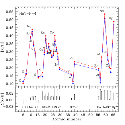
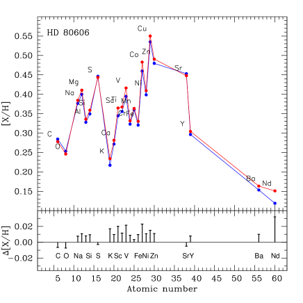
Figure 1: Chemical pattern derived using the classical solar-scaled method (red) and the new method (blue). The small lower panels show the abundance differences between both methods, being a chemical pattern difference. Upper and lower figures correspond to the stars HAT-P-4 and HD 80606.

We present in the Table 2 the final stellar parameters derived using the new scheme proposed here, together with the individual errors showed as T${}_{\rm{eff}}\pm\xi_{Teff}$, log g $\pm\xi_{logg}$, etc. The errors were derived following the same procedure of previous works, taking into account independent and covariance terms in the error propagation (see e.g. Section 3 of Saffe et al., 2015, for more details). In addition, between parentheses we show the difference between both procedures (as new method $-$ solar-scaled method). The higher differences in T_eff, log g, [Fe/H] and v_micro amount to (absolute values) 26 K, 0.05 dex, 0.020 dex and 0.05 km/s. However, it is interesting to separate the results of main-sequence and giant stars, which seem to show a slightly different behaviour. For instance, there is no evolved star with a T_eff difference higher than $\sim$10 K, while many main-sequence objects are above this value. A similar effect is seen in the average v_micro differences: there is no giant star with a v_micro difference higher than 0.02 km/s, while many main-sequence objects are above this value. On the other hand, there is no clear difference in the average difference values of main-sequence and giant stars when comparing log g and [Fe/H] values. We also note that the higher difference in T_eff corresponds to a main-sequence star (HAT-P-4 with 26 K), while the higher difference in [Fe/H] corresponds to an evolved object (HD 32887 with 0.020 dex).

In general, the differences obtained between the solar-scaled and the new method, are comparable to the individual dispersions of the values of the stellar parameters. In particular, we note that some [Fe/H] differences are higher or similar than the dispersions. For the other three stellar parameters (T_eff, log g and v_micro) the differences are usually lower than the individual dispersions. This means that the use of the non-solar-scaled method is not neccesarily mandatory for every determination of stellar parameters. However, there are some physical processes that claim a higher precision in order to be well described. We discuss specifically the significance of these differences in the Section 5.1.

Given the differences found in stellar parameters between both methods showed in the Table 2, we should expect small differences (although not identical) model structures derived using both methods. We present in the Figure 2 four examples comparing solar-scaled (blue dashed lines) and non-solar-scaled (red continuous lines) ATLAS12 model atmospheres. This Figure include two main-sequence stars (HD 19994, HAT-P-4) and two giant stars (HD 32887, HD 115659). For each star, we show the temperature T and pressure P both as a function of the Rosseland depth $\tau_{Ross}$, as derived from the ATLAS12 model atmospheres. We included intentionally the star HD 19994 in these plots, which shows one of the lowest differences in stellar parameters when derived using both methods (see Table 2). The temperature distributions using both methods are similar in general. However, the small insets present a zoom of the temperature distribution, showing indeed that the distributions are not identical: HD 19994 shows a slightly higher T for the solar-scaled method than the new method, while the other three stars shows a lower T for the solar-scaled method i.e. the contrary difference. This corresponds directly to the slightly higher and lower T_eff respectively, obtained with both methods for these stars (see Table 2). In other words, a slightly higher T distribution corresponds to a slightly higher T_eff. In the same Figure 2, we also see that the pressure distributions show a more noticeable difference when calculated using both methods. In particular, the lowest difference corresponds in this example to HD 19994, showing one of the lowest differences in parameters in the Table 2. We note that the small differences found between the models showed in the Figure 2 include the range -1 $<$ log $\tau_{Ross}$ ¡ 1 where we expect that most non-saturated spectral lines should form. Then, the plots of Figure 2 show that the structure of the model atmospheres, as expected, are similar but not identical (even for stars such as HD 19994), and the differences correspond to the differences found in stellar parameters showed in the Table 2.

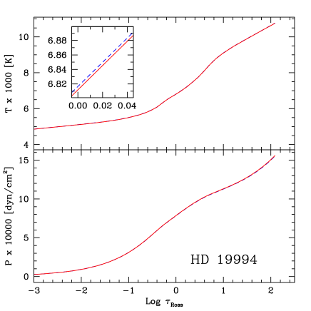
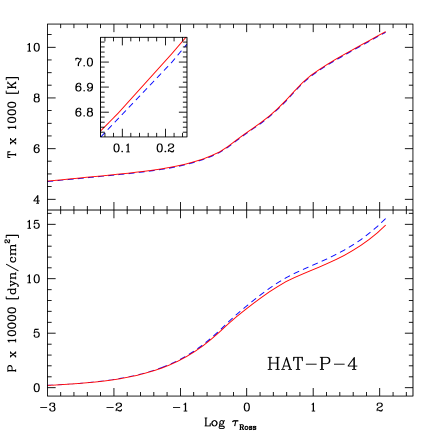
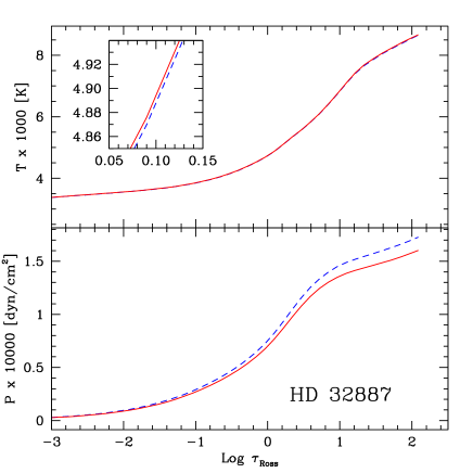
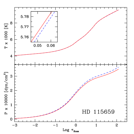
Figure 2: Comparison of solar-scaled (blue dashed lines) vs non-solar-scaled (red continuous lines) ATLAS12 model atmospheres. The example shows temperature and pressure distributions of four different stars (see text for details).

We also performed the following experiment. Using non-solar-scaled opacities, we derived the abundances of Fe I and Fe II but applying the solution found with the solar-scaled method. We present in the Figure 3 the corresponding results, showing the iron abundance vs excitation potential and iron abundance vs reduced EW for the star HAT-P-4 (upper and lower panels). Filled and empty points correspond to Fe I and Fe II, while the dashed line shows a linear fit to the abundance values. Inspecting the plots, it is clear that the four conditions required to find an appropriate solution for the model atmosphere (see Section 4) are not satisfied simultaneously. The average Fe II abundance is higher than the Fe I average (0.24 and 0.21 dex, respectively), with 8/10 Fe II lines above the Fe I average. Also, the abundances do present a slight trend with the reduced equivalent widths (lower panel). Even admitting a null slope in both panels of Figure 3, the fact that only one condition is not verified (e.g. the ionization balance), is enough to show that the stellar parameters using the solar-scaled method indeed were not exactly derived, and then a new solution could improve the previous one. And this new solution will need to change the four stellar parameters, not only one, because the four mentioned conditions are not independent between them. This task is done by the downhill simplex method within the FUNDPAR program, using non-solar-scaled opacities as explained in the Section 4.

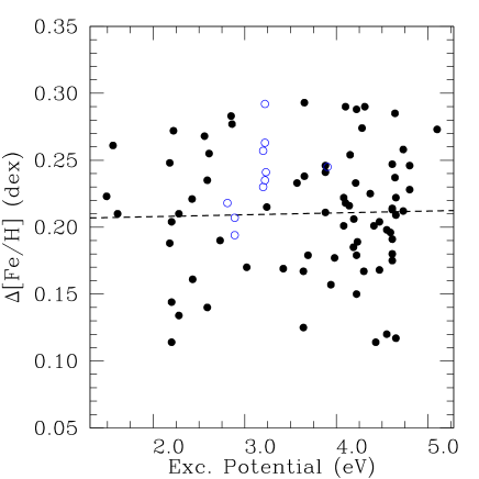
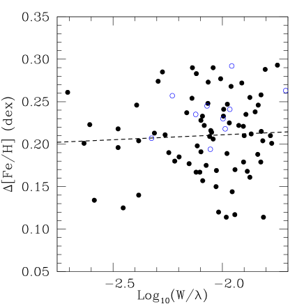
Figure 3: Iron abundance vs excitation potential (upper panel) and iron abundance vs reduced EW (lower panel) for the star HAT-P-4, derived with non-solar-scaled opacities but applying the solution of the solar-scaled method. Filled and empty points correspond to Fe I and Fe II, respectively. The dashed line is a linear fit to the abundance values. See text for more details.

From Table 2, we note that four main-sequence stars show a negative difference in T_eff between both methods (HD 19994, HD 221287, HD 96568 and HD 128898), being the stars with the highest T_eff in the main-sequence sample. Then, we wonder if the differences between both methods depend only on one parameter such as e.g. T_eff. HAT-P-4 and HD 80606 differ both by $\sim$+25 K when using both methods but having a T_eff difference of $\sim$485 K. Also, TYC 2567-744-1 and HD 80607 differ by $\sim$+15 K between both methods and have a T_eff difference of $\sim$550 K. Then, we cannot adopt solely T_eff as a proxy for the differences between both methods, although it seems to play a role. Due to the explicit calculation of the opacities for specific composition, we should expect that the differences also depend on the detailed chemical composition of each target.

We note that the differences in [Fe/H] between both methods are very similar when considering two stars in the same binary system. For instance, HD 80606 and HD 80607 present differences of +0.009 and +0.006 dex, while $\zeta^{1}$ Ret and $\zeta^{2}$ Ret present differences of +0.010 and +0.009 dex. This implies that the mutual difference in [Fe/H] between binary components is approximately preserved when considering two very similar stars.

The last two columns in the Table 2 show the slope of abundance vs condensation temperature T_c, using abundances of the classical solar-scaled method (slope s_classic) and abundances with the new scheme (slope s_new). Condensation temperatures were taken from the 50% T_c values derived by Lodders (2003) for a solar system gas with [Fe/H]=0. In particular for the binary systems of Table 2, if one star presents a higher s_classic value than its binary companion, then the same star also presents a higher slope s_new in the new method. Then, the T_c trends of previous works (SA15, SA16, SA17) are verified. However, we consider that this is not neccesarily the rule, because both slopes s_classic and s_new present small but noticeable differences between them in general, differences which are comparable to the error of the slopes and then cannot be totally ignored.

From Table 2, the values of s_new and s_classic values are similar within their errors, showing in general lower differences for giants than for main-sequence stars. Some slopes of the T_c trends remains almost identical (e.g. s_new and s_classic of HD 2114 are 3.03$\pm$1.87 and 3.06$\pm$1.87), while other T_c trends could change up to $\sim$100% of their original slopes (e.g. s_new and s_classic of HD 80606 are 2.38$\pm$0.94 and 4.17$\pm$0.85). We note that main-sequence stars with lower T_eff seem to show higher s_new values than s_classic, while stars with T_eff higher than $\sim$6200 K seem to show the contrary effect. For giant stars, those stars with T_eff lower than $\sim$4500 K seem to show s_new greater than s_classic, while for higher T_eff the behaviour is less clear. Then, the exact difference between the T_c trends depends on the fundamental parameters of the stars and of their chemical patterns.

Table 2: Stellar parameters derived using the new doubly-iterated method. The difference between both procedures is indicated with parentheses (as new method $-$ solar-scaled method).

Star	Teff	log g	[Fe/H]	vmicro	sclassic	snew
	[K]	[dex]	[dex]	[km/s]	[10-5 dex/K]	[10-5 dex/K]
Main-sequence stars
HAT-P-4	6064$\pm$35 ($+$26)	4.34$\pm$0.08 ($-$0.01)	$+$0.220$\pm$0.005 ($+$0.009)	1.30$\pm$0.09 ($+$0.04)	$+$12.37$\pm$1.53	$+$13.70$\pm$1.50
TYC 2567-744-1	6055$\pm$37 ($+$15)	4.37$\pm$0.07 ($-$0.01)	$+$0.104$\pm$0.006 ($+$0.012)	1.22$\pm$0.10 ($+$0.02)	$+$3.98$\pm$0.81	$+$5.29$\pm$0.95
HD 80606	5579$\pm$28 ($+$25)	4.31$\pm$0.10 ($+$0.02)	$+$0.268$\pm$0.002 ($+$0.009)	0.91$\pm$0.07 ($+$0.04)	$+$2.38$\pm$0.94	$+$4.17$\pm$0.85
HD 80607	5505$\pm$34 ($+$16)	4.29$\pm$0.11 ($+$0.01)	$+$0.249$\pm$0.004 ($+$0.006)	0.88$\pm$0.09 ($+$0.03)	$+$3.23$\pm$0.64	$+$4.30$\pm$0.55
$\zeta^{1}$ Ret	5725$\pm$29 ($+$11)	4.50$\pm$0.05 ($+$0.00)	$-$0.251$\pm$0.003 ($+$0.010)	0.94$\pm$0.05 ($+$0.05)	$+$2.67$\pm$1.26	$+$2.81$\pm$1.21
$\zeta^{2}$ Ret	5874$\pm$27 ($+$13)	4.52$\pm$0.07 ($-$0.01)	$-$0.270$\pm$0.004 ($+$0.009)	1.08$\pm$0.06 ($+$0.05)	$-$2.31$\pm$1.37	$-$0.84$\pm$1.34
HD 19994	6245$\pm$39 ($-$4)	4.42$\pm$0.15 ($+$0.00)	$+$0.228$\pm$0.010 ($-$0.001)	1.38$\pm$0.11 ($-$0.01)	$-$2.82$\pm$1.37	$-$3.51$\pm$1.37
HD 221287	6340$\pm$40 ($-$6)	4.63$\pm$0.13 ($+$0.01)	$+$0.007$\pm$0.010 ($-$0.001)	1.28$\pm$0.12 ($-$0.01)	$+$7.60$\pm$1.48	$+$7.47$\pm$1.47
HD 96568	8333$\pm$39 ($-$14)	3.59$\pm$0.09 ($+$0.04)	$-$0.081$\pm$0.005 ($+$0.010)	1.54$\pm$0.08 ($+$0.02)	$+$6.56$\pm$4.77	$+$6.40$\pm$4.77
HD 128898	8035$\pm$27 ($-$8)	4.64$\pm$0.09 ($+$0.02)	$+$0.099$\pm$0.008 ($+$0.008)	1.59$\pm$0.11 ($-$0.03)	$+$7.99$\pm$4.82	$+$6.59$\pm$4.84
Evolved stars
HD 2114	5308$\pm$35 ($-$8)	2.87$\pm$0.12 ($-$0.03)	$-$0.047$\pm$0.010 ($+$0.000)	1.86$\pm$0.10 ($-$0.01)	$+$3.06$\pm$1.87	$+$3.03$\pm$1.87
HD 10761	5036$\pm$32 ($+$8)	2.74$\pm$0.10 ($-$0.03)	$+$0.018$\pm$0.007 ($+$0.005)	1.49$\pm$0.09 ($+$0.01)	$+$7.04$\pm$2.50	$+$7.22$\pm$2.46
HD 28305	5020$\pm$41 ($+$1)	3.00$\pm$0.11 ($+$0.01)	$+$0.157$\pm$0.006 ($+$0.004)	1.72$\pm$0.11 ($-$0.01)	$+$9.36$\pm$2.68	$+$9.42$\pm$2.66
HD 32887	4271$\pm$39 ($+$6)	1.91$\pm$0.12 ($-$0.04)	$-$0.169$\pm$0.006 ($+$0.020)	1.57$\pm$0.08 ($+$0.00)	$+$6.62$\pm$3.10	$+$7.47$\pm$3.10
HD 43023	5069$\pm$29 ($-$7)	3.05$\pm$0.11 ($+$0.01)	$-$0.020$\pm$0.004 ($-$0.001)	1.25$\pm$0.05 ($-$0.02)	$+$4.44$\pm$1.82	$+$3.64$\pm$1.81
HD 50778	4131$\pm$39 ($+$7)	1.62$\pm$0.16 ($-$0.05)	$-$0.431$\pm$0.007 ($+$0.014)	1.60$\pm$0.10 ($+$0.00)	$+$4.42$\pm$3.08	$+$5.34$\pm$3.10
HD 85444	5179$\pm$31 ($+$2)	2.97$\pm$0.14 ($-$0.01)	$+$0.051$\pm$0.010 ($+$0.004)	1.47$\pm$0.07 ($+$0.00)	$+$5.61$\pm$2.02	$+$7.72$\pm$2.08
HD 109379	5240$\pm$36 ($+$5)	2.75$\pm$0.15 ($+$0.00)	$-$0.003$\pm$0.006 ($+$0.005)	1.75$\pm$0.13 ($+$0.00)	$-$1.80$\pm$2.35	$-$1.50$\pm$2.35
HD 115659	5159$\pm$29 ($+$4)	2.94$\pm$0.13 ($-$0.02)	$+$0.066$\pm$0.008 ($+$0.004)	1.49$\pm$0.07 ($+$0.00)	$+$8.74$\pm$2.28	$+$9.03$\pm$2.26
HD 152334	4291$\pm$37 ($+$5)	2.11$\pm$0.12 ($-$0.01)	$-$0.072$\pm$0.005 ($+$0.010)	1.41$\pm$0.11 ($-$0.01)	$+$5.92$\pm$3.04	$+$6.67$\pm$3.56

5.1 Solar-scaled or not: are the differences significant?

At first view, a difference of 0.01 dex in metallicity or 15 K in T_eff does not seem to be significant. For instance, a number of works show that giant planets form preferentially around metal-rich stars (e.g. Santos et al., 2004, 2005; Fischer & Valenti, 2005), which is called the giant planet-metallicity correlation. In these statistical works with hundreths of objects, an individual dispersion in [Fe/H] of 0.01 or 0.02 dex would not be significant. However, exoplanet host stars are a fossil record of planet formation, beyond the giant planet-metallicity correlation. Using a high-precision abundance analysis, Meléndez et al. (2009) found a lack of refractories in the atmosphere of the Sun, when compared to the average abundances of 11 solar twins. The authors found a trend between the abundances and T_c of the different chemical species, as a possible signature of rocky planet formation. They proposed that the refractory elements absent in the Sun’s atmosphere were used to create rocky planets and the nuclei of giant planets. This idea was followed by a number of works in literature (see e.g. Ramírez et al., 2010; Tucci Maia et al., 2014; Saffe et al., 2015, 2016, 2017). The detection of this planetary chemical signature is a very challenging task, requiring a careful and detailed analysis of the data, as we explain below.

The complete T_c trend detected by Tucci Maia et al. (2014) for the stars of the binary system 16 Cyg, covers a range of only 0.04 dex between the maximum and minimum abundance values of 19 different chemical species (see their Figure 3). We showed previously (Figure 1) that a number of species suffer an abundance difference (as new method $-$ solar-scaled) higher than the $\sim$0.01 dex of the [Fe/H], reaching up to $\sim$0.03 dex for e.g. Nd or Sm in HAT-P-4, with some elements showing even the contrary difference (such as C and O). Then, it is clear that the inclusion or not of this effect will have an important impact in the detection of a possible T_c trend, in objects such as the stars of the 16 Cyg binary system, where the complete trend covers only 0.04 dex. This shows that the detection of a possible T_c trend (as a chemical signature of planet formation) requires the maximum achievable precision in both stellar parameters and abundances. In general, we can say that those high-precision studies whose results depend on the mutual comparison of different chemical species should prefer the non-solar-scaled method.

It is also notable that our Sun is considered a typical star in the context of the giant planet-metallicity correlation, however the same Sun do shows a clear T_c trend when compared to solar twins (Meléndez et al., 2009; Ramírez et al., 2010) using very high-precision abundances. This apparent dichotomy derive in part from the precision reached in these different works. It would be very difficult (if not impossible) to detect a slight T_c trend by applying only standard techniques (e.g. non-differential) rather than high-precision methods of stellar parameters derivation.

The search of a possible chemical signature of planet formation is not the only reason to pursuit high-precison stellar parameters. Several examples in the literature shows that, for instance, a precise planetary characterization depends on the precise derivation of stellar parameters. For instance, Bedell et al. (2017) revised the stellar parameters of the host star Kepler-11 using a high-precision spectroscopic method and showed that the planet densities raised between 20% and 95% per planet compared to previous works. Other example corresponds to the derivation of the planetary radius which depends on the stellar radius, which in turn is derived from the fundamental parameters T_eff, log g, [Fe/H] and v_micro (see e.g. Johnson et al., 2017). Notably, the improved derivation of parameters allowed the detection of a gap in the radius distribution of small planets (R $<$ 2 R_Earth, Fulton et al., 2017), showing the possible presence of two different populations of planets (rocky planets and Neptune-like planets). Then, the importance of precise stellar parameters is evident. Also, we can consider the missing mass of refractory material in the atmosphere of the stars due to the planet formation process, estimated using the models of Chambers (2010). Using the solar-scaled results for the star HAT-P-4 we obtain M_rock $=$ 7.2 $\pm$ 0.4 M_Earth, while using the non-solar-scaled values we derive M_rock $=$ 8.6 $\pm$ 0.4 M_Earth i.e. a 20% of difference. This error could be avoided using the new estimation of parameters. Then, it is clear the need for reach the highest possible precision in these works.

Following the previous considerations, we can summarize as follows. If we are working with a large sample of stars, trying only to detect e.g. a global difference in metallicity of $\sim$0.20 dex between two subgroups, then an individual dispersion of $\sim$0.01 dex does not seem to be significant. On the other hand, if we are trying to detect e.g. a relative difference in abundances of different species (such as a T_c trend) or e.g. the missing mass of refractory material due to the planet formation process, then it is worthwhile to use the highest possible precision. It is also important to keep in mind that some chemical species show differences higher than that of [Fe/H]. We caution that the use of a lower precision will certainly tend to mask or smooth out the signal of any physical process which requires a higher precision to be detected.

5.2 A bias in studies of many stars?

From Table 2, although T_eff seems to play a role, it is not clear that a single parameter determines the differences between the two methods. However, we can suppose that a group of stars in the solar neighborhood presents a chemical pattern approximately similar to the solar one, while other stars have in general a non-solar-scaled pattern. Suppose that we obtain stellar parameters for all stars using the classical two-step method and the non-solar-scaled method. Then, those stars in the first group will show similar parameters derived with both methods, given their chemical pattern approximately solar. However, those stars in the second group will present a difference in their parameters, which gradually increases as stars present patterns farther and farther from the solar one. This would correspond to a possible small bias in the parameters, depending on the chemical composition of the stars considered. In addition, Castelli (2005a) showed that the internal temperature distribution T vs log $\tau_{Rosseland}$ of ATLAS9 and ATLAS12 model atmospheres do differ with increasing T_eff, adopting in principle the same abundance pattern in both cases. Then, we consider that a possible small bias cannot be totally ruled out. We will address this important question in detail quantitatively in a next work.

6 Conclusion

We used non-solar-scaled opacities for a simultaneous derivation of stellar parameters and chemical abundances in a sample of solar-type main-sequence and evolved stars. To date, this is probably one of the more precise spectroscopic methods of stellar parameters determination. The difference in stellar parameters could amount to +26 K in T_eff, 0.05 dex in log g and 0.020 dex in [Fe/H], when using solar-scaled vs non-solar-scaled methods. We note that some chemical species could also show a variation higher than those of the [Fe/H], and varying from one specie to another, obtaining a chemical pattern difference between both methods. This means that T_c trends could also present a variation. The differences were derived using the full line-by-line differential technique i.e. both for the derivation of stellar parameters and chemical abundances. We consider that the use of non-solar-scaled opacities is not neccesarily mandatory e.g. in statistical studies with large sample of stars. On the other hand, those high precision studies whose results depend on the mutual comparison of different chemical species (such as a T_c trend) should prefer the non-solar-scaled method. In these cases, when modeling the atmosphere of the stars, the four stellar parameters usually taken as (T_eff, log g, [Fe/H], v_micro) should in fact be considered as (T_eff, log g, chemical pattern, v_micro), which is conceptually closer to the real case.