marginparsep has been altered.
topmargin has been altered.
marginparwidth has been altered.
marginparpush has been altered.
The page layout violates the ICML style.
Please do not change the page layout, or include packages like geometry,
savetrees, or fullpage, which change it for you.
We’re not able to reliably undo arbitrary changes to the style. Please remove
the offending package(s), or layout-changing commands and try again.
No Multiplication? No Floating Point? No Problem!
Training Networks for Efficient Inference
Anonymous Authors1
Abstract
For successful deployment of deep neural networks on highly resource constrained devices (hearing aids, earbuds, wearables), we must simplify the types of operations and the memory/power resources required during inference. Completely avoiding inference-time floating point operations is one of the simplest ways to design networks for these highly constrained environments. By quantizing both our in-network non-linearities and our network weights, we can move to simple, compact networks without floating point operations, without multiplications, and without non-linear function computations. Our approach allows us to explore the spectrum of possible networks, ranging from fully continuous versions down to networks with bi-level weights and activations. Our results show that quantization can be done with little or no loss of performance on both regression tasks (auto-encoding) and multi-class classification tasks (ImageNet). The memory needed to deploy our quantized networks is less than one-third of the equivalent architecture that uses floating-point operations. The activations in our networks emit only a small number of predefined, quantized values (typically 32) and all of the network’s weight are drawn from a small number of unique values (typically 100-1000) found by employing a novel periodic adaptive clustering step during training.
1 Introduction
Almost all recent neural-network training algorithms rely on gradient-based learning. This has moved the research field away from using discrete-valued inference, with hard thresholds, to smooth, continuous-valued activation functions Werbos (1974); Rumelhart et al. (1986). Unfortunately, this causes inference to be done with floating-point operations, making it difficult to deploy on an increasingly-large set of low-cost, limited-memory, low-power hardware in both commercial Lane et al. (2015) and research settings Bourzac (2017).
Avoiding all floating point operations allows the inference network to realize the power-saving gains available with fixed-point processing Finnerty & Ratigner (2017). To move fully to fixed point, we need to quantize both the network weights and the activation functions. We can also achieve significant memory savings, by not just quantizing the network weights, but clustering all of them across the entire network into a small number of levels. With this in place, the memory footprint grows about (or less) as fast as the unclustered, continuous-weight network size. Additionally, the relative rates at which our memory footprint will grow is easily controlled using , the number of unique weights. In our experiments, with , we show that we can meet or exceed the classification performance of an unconstrained network, using the same architecture and (nearly) the same training process.
While most neural networks use continuous non-linearities, many use non-linearities with poorly defined gradients, without impacting the training process Nair & Hinton (2010); Glorot et al. (2011); Goodfellow et al. (2013). When purely quantized outputs are desired, however, such as with binary units, a number of additional steps are normally taken Bengio et al. (2013); Tang & Salakhutdinov (2013); Raiko et al. (2014); Courbariaux et al. (2016); Maddison et al. (2016); Hou et al. (2016) or evolutionary strategies are used Plagianakos et al. (2001). At a high level, many of the methods employ a stochastic binary unit and inject noise during the forward pass to sample the units and the associated effect on the network’s outputs. With this estimation, it is possible to calculate a gradient and pass it through the network. One interesting benefit of this method is its use in generative networks in which stochasticity for diverse generation is desired Raiko et al. (2014). Raiko et al. (2014) also extended Tang & Salakhutdinov (2013) to show that learning with stochastic units may not be necessary within a larger deterministic network.
A different body of research has focused on quantizing and clustering network weights Yi et al. (2008); Courbariaux et al. (2016); Rastegari et al. (2016); Deng et al. (2017); Wu et al. (2018). Several existing weight-quantization methods (e.g., Courbariaux et al. (2016)) liken the process to Dropout Srivastava et al. (2014) and its regularization effects. Instead of randomly setting activations to zero when computing gradients (as with dropout), weight clustering and binarization tends to push extreme weights partway back towards zero. Additional related work is given in the next section.
2 Training Networks for Efficient Inference
In this section, we separately consider the tasks of (1) quantizing the output of each unit and (2) reducing the set of allowed weights to a small, preset, size. The effects of each method are examined in isolation and together in Section 3.
2.1 Activation Quantization
Figure 1 gives a simple procedure that we use for activation quantization.111 For the research reported in this paper, we use equal step sizes in the activation-output space (see Figure 1). However nothing in our final system requires this. To make this section concrete and easily reproducible, we show the effects of quantization on tanh’s output. However, we have employed the exact same method to quantize ReLU-6 Krizhevsky & Hinton (2010), rectified-tanh, and sigmoid among others.
function gammaD (input, levels): y step quant_y return quant_y

Naively backpropagating errors with these quantized tanh (tanhD) units will quickly run into problems as the activations are both discontinuous and characterized by piece-wise constant functions. In order to use gradient-based methods with tanhD units, we need to define a suitable derivative. We simply use the derivative of the underlying function — (e.g. for , we used ). In the forward pass, both in training and inference, the output is quantized to levels. In the backward pass, we proceed by ignoring the quantization and instead compute the derivatives of the underlying function. Whereas previous studies that attempted quantization to binary-output units experienced difficulties in training, we have found that as is increased, even to relatively small values (), all of the currently popular training algorithms perform well with no modification Baluja (2018), (e.g. SGD, SGD+momentum, ADAM, RMS-Prop, etc). A number of studies have used similar approaches, often in a binary setting (e.g. straight through estimators Hinton (2012); Bengio et al. (2013); Rippel & Bourdev (2017)); most recently, Agustsson et al. (2017); Mentzer et al. (2018) used a smooth mixture of the quantized and underlying function in the backwards pass.
Why does ignoring the quantization in the backwards pass work? If we had tried to use the quantized outputs, the plateaus would not have given usable derivatives. By ignoring the quantizations, the weights of the network still move in the desired directions with each backpropagation step. However, unlike non-quantized units, any single move may not affect the unit’s output. In fact, it is theoretically possible the entire network’s output may not change despite all the weight changes made in a single step. Nonetheless, in a subsequent weight update, the weights will again be directed to move, and of those that move in the same direction, some will cause a unit’s output to cross a quantization threshold. This changes the unit’s and, eventually, the network’s output. Further, notice that for tanhD, Figure 1, the plateaus are not equally sized. Where the magnitude of the derivative for the underlying tanh function is maximum is where the plateau is the smallest. This is beneficial in training since the unit’s output changes most rapidly where the derivative of tanh changes the most rapidly.
Finally, to provide an intuitive example of how these units perform in practice, see Figure 2. This shows how a parabola is fit with a variety of activations and quantization. In this example, a tiny network with a single linear output unit and only two hidden units is used. The most revealing graphs are the training curves with tanhD() (Figure 2-c). The fit to the parabola matches closely with intuition; the different levels of quantization symmetrically reduce the error in a straightforward manner. As is increased (d and e), the performance approximates and then matches the networks trained with tanh and ReLU activations.
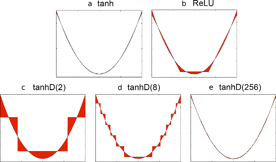
To summarize, a simple procedure to quantize the outputs of a unit’s activations was given. For ease of exposition and clarity, it was presented with tanh, though testing has been done with most, if not all, the commonly used activation functions. Beyond tanhD, we will demonstrate the use of quantized ReLU activations in Section 3.
2.2 Weight Quantization
We turn now to reducing the set of allowed weights to a small, predefined, number. As the goal of our work is efficient inference; we do not attempt to stay quantized during the training process. The process used to obtain only a small number of unique weights is a conceptually simple addition to standard network training. Like activation quantization, it can be used with any weight setting procedure - from SGD or ADAM to evolutionary algorithms.
Previous research has been conducted in making the network weights integers Yi et al. (2008); Wu et al. (2018), as well as reducing the number of weights to only binary or ternary values Courbariaux et al. (2016); Deng et al. (2017) during both testing and training, using a stochastic update process driven by the sign bit of the gradient. Empirically, many of the previous techniques that either compress or quantize weights on an already trained model perform poorly on real-valued regression problems. While our implementations of Denton et al. (2014); Han et al. (2016); Lin et al. (2015) are quite successful on classification problems, we were unable to achieve comparable performance using those techniques on networks that perform image compression and reconstruction, using the architectures described in Ballé et al. (2016). We hypothesize that the reason for this is that quantizations can create sharp cuts that seem to be beneficial for decision boundaries but hinder performance when regressing to real-valued variables. Tasks in which real-valued outputs are required have become common recently (e.g. image-to-image-translation Isola et al. (2016), image compression and speech synthesis, to name a few). Fortunately, our method exhibits good performance on regression tasks, as well as providing an easily tunable hyper-parameter (the number of weight clusters), thereby alleviating any remaining task impact.
Perhaps the most straightforward approach to creating a network with only a limited number of unique weights () is to start with a trained network and quantize the weights to a small number, , of equally spaced values. While this clearly allows us to use fixed-point arithmetic, this approach has limitations. The number of uniformly spaced levels must be large to retain good performance: Lin et al. (2015) showed that, even with 1024 distinct (equally-spaced) levels on the first layer of Alexnet, straightforward quantization (without post-quantization fine tuning) resulted in a classification accuracy drop of 72%.222This number is based on Lin et al. (2015) Figure 4 “optimized bit-width” with conv1 weights having distinct values; conv2 and conv4 each having distinct values; and conv3, conv5, fc1 and fc2 each having distinct values. The total number of distinct weight values within the network would be 1344. As will be explained in Section 4, moving away from uniform quantization does not force us away from fixed-point arithmetic: we are able to reap the power/computational benefits of this regime without resorting to uniform sampling.
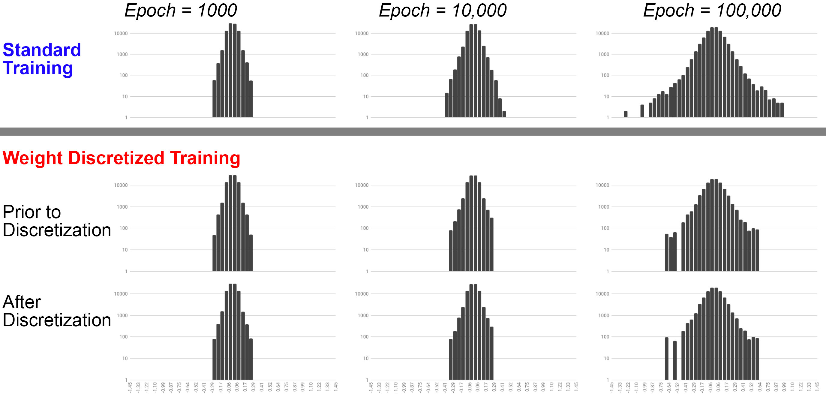
To address the limitations in uniform quantization, we instead adaptively cluster the weights throughout the training process. Rather than fully training a network and then quantizing the weights, a recurring clustering step is added into the training procedure. Periodically (after every 1000 steps, in our experiments), all of the weights in the network, including the bias weights, are clustered in a one-dimensional (the value of the weight/bias) k-means process Jain (2010).333 All of the clustering approaches that we tried (e.g., LVQ Kohonen (1995), HAC Duda et al. (1995), k-means) gave similar results. We used k-means for simplicity. Clustering, rather than using uniformly sized bins, ensures that bin spacing respects the underlying distribution of the weights (Figure 3).
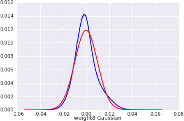
As will be seen in our results (Section 3), using k-means clustering on the weights and biases of small- and medium-sized networks works extremely well. However, k-means clustering on more than about a million parameters can become prohibitively slow, even though we only do this clustering once every one thousand steps. Most modern networks far surpass a million weights: Alexnet, for example, has more than 50 million weights and biases. In Section 3.3, we use a simple method to sidestep this problem by subsampling in the weight/bias space, and determine cluster centers using only 2% of the parameters. This subsampling allows for faster training, but does not make use of the available information about the weight/bias distributions and, as we will see in Section 3.3, gives about 3% lower network accuracy.
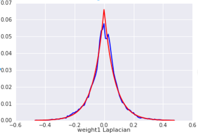
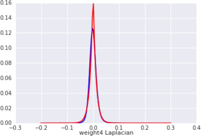
Instead of simply subsampling, we can make use of what we know about fully-trained weight distributions: that many resemble Laplacian or Gaussian distributions. Figure 3 shows this for a fully-trained MNIST-classification network and Figure 4 shows it for the fully-trained Alexnet. This insight opens interesting model-based approaches to quantization. Specifically, if the “natural” (unquantized) weight/bias distributions on large networks really should be Laplacian (or Gaussian), the loss in accuracy of the quantized network might be traced back to the overall or error of the quantized weights/biases compared to their “natural” distributions. Under this assumption, we should be able to determine the optimal quantization levels based on these parameterized models. Figure 5 shows cluster centers and occupancies for Laplacian distributions that minimize its or error in the weight/bias space. While this does not necessarily correspond directly to minimizing the accuracy loss, using the Laplacian not only matched the classification accuracy than we got from unconstrained k-means, but actually surpassed it, as we will show in Section 3.3.
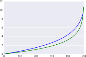
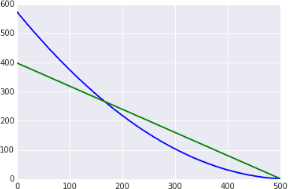
One interesting characteristic of the Laplacian-based clustering model is that we can describe the best cluster center locations in closed form, as a function of the extreme values that were seen in the sampled set. Specifically, for minimum error and using an odd number of cluster centers, the cluster centers should be at where is the mean value of the network weights and is a scaling factor and where with and . We set the scaling factor, , using the cluster occupancy curve for guidance. From Figure 5, for minimum error on a fair sample set from a Laplacian distribution, occupancy of the clusters should fall linearly. However, early in training, the observed weight distribution is far from a fair Laplacian sample: many more weights are near zero than dictated by a Laplacian model. We adjust for this by setting so that, early in training, the maximum quantization level is at or slightly beyond the maximum observed weight. Specifically, we start with where is the maximum amplitude difference between any weight and the mean . This scaling allows us to accurately model the largest magnitude weights.
On a pragmatic note, we found that in the beginning of training, the weights were too tightly clustered around the mean (compare the left and right columns in Figure 3). We determined that by slightly “nudging” in early training, we could speed-up convergence without losing final network accuracy. If , we change to move outward by . Later in training, tying our scaling parameter to means that we would lose the regularization benefits seen in Figure 3-b and -c. To avoid losing that, we “nudge” the value of just slightly lower, by , whenever the activation weights are spread out by more than the expected range of desired values (specifically, whenever ). We will revisit this Laplacian-model–based approach with our investigation of Alexnet (Section 3.3).
2 Hidden Layers


(a) Activations quantized
4 Hidden Layers

(b) Weights quantized
(c) Both quantized
Whichever way we pick the quantization clusters (whether using k-means or model-based approaches), once the clusters are created, each weight is replaced with the centroid of its assigned cluster, thereby reducing the number of unique weights to . After weight replacement, training continues with no modifications until the next clustering step. At this point, the cycle repeats. For all of our experiments, quantization occurs after every 1000 training steps.
This procedure, though simple, has some subtle effects. First, as a training regularizer, it keeps the range of the weights from growing too quickly, as there is a persistent “regression to the mean.” Second, it provides a mechanism to inject directed noise into the training process. As we will show, both of these properties have, at times, yielded improved results over allowing arbitrary valued weights. Figure 3 (row b) shows the distribution of weights at the beginning, middle, and end of training when weight clustering is used, immediately prior to the quantization step. With 1000 clusters used throughout training, the weights after replacement (Figure 3, row c) appear very similar to the unclustered weights (Figure 3, row b).
3 Experiments
We experimented with many tasks and network architectures to determine how quantizations of activations and weights affected performance. These experiments included testing memorization capacity, real-value function approximation, and numerous classification problems. Because of space limitations, however, we only present the three most often researched tasks; these are representative of the results seen across our studies. We present two classification tasks: MNIST LeCun et al. (1998), and ImageNet Russakovsky et al. (2014). We also present a real-valued output task: auto-encoding images, the crucial building block to neural-network based image compression.
In all of our tests, we retrained the baselines to eliminate the possibility of any task-specific heuristics. In some cases, this led to lower baseline performance than state-of-the-art; however, since our goal is to measure the relative effect of quantizations on any network, the results provide the insights needed.
3.1 MNIST
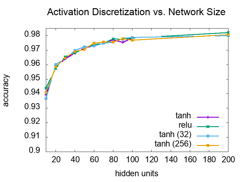
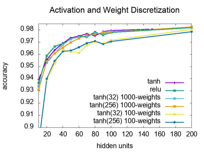
For MNIST, we train a fully connected network with ADAM Kingma & Ba (2015) and vary the number of hidden units to explore the trade-off between quantization, accuracy, and network size. These networks ranged from just over 8,000 parameters up to nearly 110,000 parameters, depending on the architecture and number of hidden units. Figure 6-a contains the performance of the networks using ReLU and tanh activation functions with no quantizations; these are the baselines. Since tanh slightly outperformed ReLU, we will quantize tanh in our experiments.

Convolution

(a) Activations quantized
Fully Connected
(b) Weights quantized

(c) Both quantized
First, we examine the effect of only quantizing each unit’s activations. We experimented with 8 sets of activation quantization (2, 4, 8, … 256 levels). We found that both tanhD(8) and tanhD(16) often perform as well as tanh and ReLU in performance when there are hidden units per layer. At tanh(32) and above, performance is largely indistinguishable from tanh (Figure 6-a). Next, we examine weight quantization in isolation using k-means clustering. Two sets of experiments are presented: and (Figure 6 b). With 1000 unique weights allowed, the performance is nearly identical to no weight quantization. However, when is reduced to 100, there is a decline in performance. Nonetheless, note that even with the performance recovers with additional hidden units – hinting towards the trade-off in representational capacity between number of distinct values a weight can represent and the number of weights in the network.
Finally, when both quantizations are combined, we again see that the only noticeable negative effect comes when the number of unique weights is set to 100. No matter which activation is used, when 100 weights are used, performance decreases. This same trend holds true for networks with a depth of 2 hidden layers (top row) and with 4 hidden layers (bottom row).
3.2 Auto-Encoding
A number of recent as well as classic research papers have used auto-encoding networks as the basis for image compression Cottrell & Munro (1988); Kramer (1991); Jiang (1999); Toderici et al. (2016); Svoboda et al. (2016); Toderici et al. (2017). To recreate the input image, real values are used as the outputs. As discussed earlier, real value approximation can be a more challenging problem domain than classification when quantizing the network.
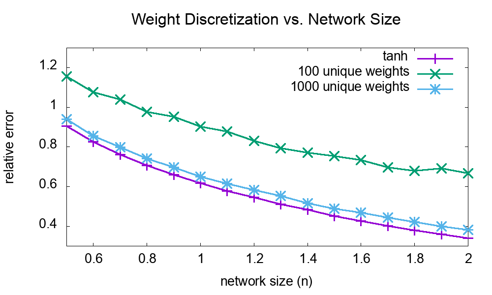
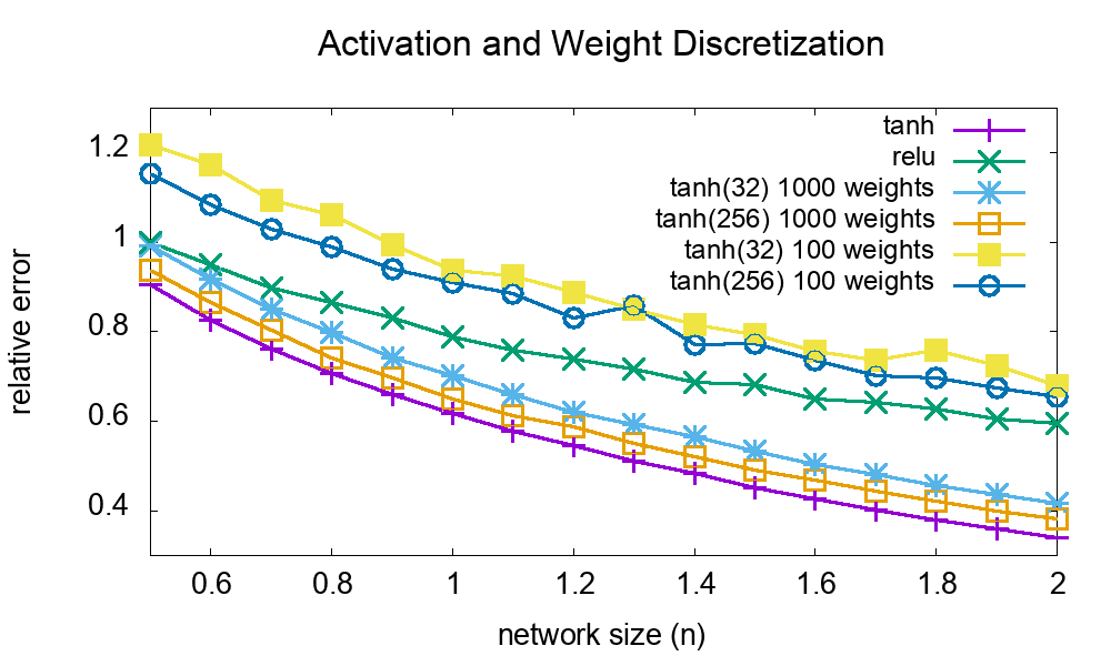
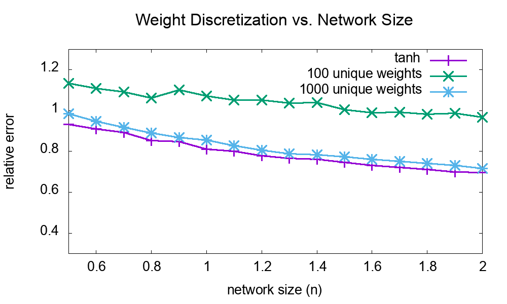
For these experiments, we train two network architectures: convolutional (26,000 to 380,000 parameters) and fully connected (160,000 to 660,000 parameters). ADAM is used for training, and error is minimized. We trained with the ImageNet train-set and all tests are performed with the validation images. The smallest conv-network has four conv. layers with (, , , ) depth, followed by 3 conv-transpose layers with depth (, , ). The last two layers are conv. with depth 20 and 3. For the second experiment, the fully-connected network has 7 hidden layers with (, , , , , ) units each. To examine the effects of network size, is varied from 0.5 to 2.0 for both experiments.
Because the raw numbers are not meaningful in isolation, we show performance measurements relative to training the smallest network with ReLU activations and no quantizations (the graphs for both architectures can be compared to see effects of network size). In Figure 7-a for both architectures, ReLU performed worse than tanh. TanhD(32) and TanhD(256) tracked the performance of tanh closely for all sizes of the network. Similarly to the MNIST experiment (Figure 6 b), reducing the number of weights to hurt performance. With , the performance decline was much smaller; however, unlike with MNIST, there was a discernible effect.
| Activation | Unique | Unquantized inputs | Quantized inputs | ||||
| Experiment | # | Levels | Weights | Recall | Recall | Recall | Recall |
| () | () | @1 | @5 | @1 | @5 | ||
| AlexNet w/ ReLU | 0 | - | - | 57.4 | 80.4 | - | - |
| AlexNet w/ ReLU6 | 1 | - | - | 56.4 | 79.8 | - | - |
| Continuous weights, only quantized activations. | 2 | 256 | - | 56.1 | 79.8 | - | - |
| 3 | 32 | - | 56.0 | 79.4 | 56.0 | 79.6 | |
| 4 | 16 | - | 55.8 | 79.4 | 55.4 | 78.9 | |
| 5 | 8 | - | 53.4 | 77.7 | 52.6 | 77.1 | |
| k-means quantized weights and quantized activations (no dropout). | 6 | 32 | 1000 | 52.5∗ | 76.3∗ | 52.1 | 76.0 |
| 7 | 32 | 100 | 48.6∗ | 73.1∗ | 47.2 | 72.2 | |
| Laplacian quantized weights, quantized activations: | |||||||
| - with dropout | 8 | 32 | 1000 | 55.5∗ | 79.3∗ | 55.5 | 79.2 |
| - without dropout | 9 | 32 | 1000 | 57.1∗ | 79.8∗ | 56.9 | 79.4 |
When the two quantizations were combined, again, the largest impact was a result of setting the weight quantization levels too low. As before, increasing the network size returns the performance lost due to weight and activation quantization. Importantly, this task indicates that although the quantization procedures do indeed take a larger toll on the performance with real-outputs, quantization remains a viable approach for network computation/memory reduction. The amount of performance degradation tolerated can be explicitly dictated by the needs of the application by controlling . It is worth repeating here that while our implementations of many of the recent competing methods in Denton et al. (2014); Han et al. (2016); Lin et al. (2015) are quite successful on classification problems, we were unable to achieve comparable performance using those techniques on compression and reconstruction.
3.3 AlexNet
To evaluate the effects of quantization on a larger network (more than 50 million parameters), we used AlexNet Krizhevsky et al. (2012) to address the 1000-class ImageNet task. To ensure that we are training our network correctly, we first retrained AlexNet from scratch using the same architecture and training procedures specified in in Krizhevsky et al. (2012); some small differences are: we employed an RMSProp optimizer, weight initializer sd=0.005, bias initializer sd=0.1, one Nvidia Tesla P100 GPU, and a stepwise decaying learning rate. Our network achieved a recall@5 accuracy of 80.4% and recall@1 accuracy of 57.4%. This should be compared to the accuracy reported in Krizhevsky et al. (2012) of 81.8% and 59.3%, recall@5 and recall@1, respectively. The small difference in performance was because we did not use the PCA pre-processing, which Krizhevsky et al. (2012) cite as causing approximately the difference seen. All of the remaining comparisons will use the exact same training procedure, only differing in which quantizations and activations are used.
To begin, we examined the effect of switching to ReLU6 instead of ReLU. AlexNet with ReLU6 achieved a recall top-1 of 56.4% and top-5 of 79.8% (Experiment #1). This change is needed to support activation quantization, to give a bounded range. With that change, we then examine the performance of only quantizing the activations and inputs, without weight quantization, in Experiments #2-#5 444 We separately report two approaches: first, quantizing activation outputs without quantizing the network inputs and, second, quantizing both activation outputs and network inputs to the same number of levels. This allows us to compare to other prior work which left the first and last layers of their networks unquantized Zhou et al. (2016); Rastegari et al. (2016).. using 256 activation levels (8 bits) down to only 8 levels (3 bits). In Experiments #2 and #3, there is little degradation in performance in comparison to using the full floating point (32 bits) (Experiment #1). Below 32 levels with both input and activation quantization (right most columns in Table 1), performance declines (Experiment #4 and #5).
Using the most aggressive acceptable activation quantization (32 values), we turn to our next experiment: reducing the number of unique weights allowed. We set (Experiment #6). The only training modification was the elimination of dropout. As illustrated in Figure 3, the quantization process itself works as a regularizer, so dropout is not needed. Wu et al. (2018) took a similar approach and removed dropout from their AlexNet quantization experiments. It should also be noted that Wu et al. (2018) did not quantize the last layer’s weights for reporting results. All of our quantized AlexNet results include quantization of the final layer’s weights. Also, Wu et al. (2018) did not quantize the network inputs – we show performance with input quantization (rightmost columns “Quantized Inputs”). For speed in training, only a randomly selected 2% sample of the full weight/bias set was used for k-means clustering; however, all the weights/bias parameters were then set to those cluster centers.
| Recall@1 | Recall@5 | |||||
| baseline | quantized | difference | baseline | quantized | difference | |
| Our work | 57.4% | 57.1% | -0.3% | 80.4% | 79.8% | -0.6% |
| WAGE Wu et al. (2018) | - | - | - | 80.7% | 75.9% | -4.8% |
| DoReFa Zhou et al. (2016) | 55.9% | 53.0% | -2.9% | - | - | - |
| QNN Hubara et al. (2016) | 56.6% | 51.0% | -5.6% | 80.2% | 73.7% | -6.5% |
| XNOR-Nets Rastegari et al. (2016) | 56.6% | 44.2% | -12.4% | 80.2% | 69.2% | -11.0% |
| Optimized fixed-point Lin et al. (2015)22footnotemark: 2 | - | - | - | 80.3% | 22.6% | -57.7% |
Examining Experiments #6 and #7, we see that Experiment #7, with only 100 unique weights, performed much better than we would have expected given its earlier performance in Subsections 3.1 and 3.2. We speculate that unlike the other tasks in which setting was detrimental to performance, AlexNet has so much extra capacity and depth that the effective decrease in representational capacity for each weight was lessened by the large architecture.
The results to this point show minimal loss in performance (relative to Experiment #1) after the activation is quantized to 32 levels and 1000 weights are used. Let us take a step-back and compare to other methods of quantization. Our results already improve on the absolute as well as relative loss in recall@5 accuracy seen in earlier studies Zhou et al. (2016); Hubara et al. (2016); Wu et al. (2018) and is close to the best previous recall@1 loss Zhou et al. (2016). However, as pointed out in Section 2.2, we might be able to do better using a model of the expected weight distribution, rather than relying on k-means clustering of a 2% sample. We chose to use a Laplacian distribution model according to -error spacing. Using this approach, we see a significant improvement in performance (Experiment #9). We surpass the performance both of our fully continuous baseline (Experiment #1) and of our k-means weight clustering (Experiment #6).
Compared to the prior work that focused on moving away from floating-point implementations (Table 2),555 We have only included in this table those references that reported their work on ImageNet classification using the Alexnet architecture, quantizing both weights and activations, so that comparisons are fair. For this reason, several well-known pieces of prior work Vanhoucke et al. (2011); Courbariaux et al. (2016); Li et al. (2017) are not included in Table 2. our approach is the only one which did not suffer a significant loss in performance, relative to the unquantized version of the network. We have, by far, the best performance both relative to baseline and in absolute terms. Han et al. (2016) is the only other reference that we have found with weight quantization that did not suffer from performance loss but Han et al. (2016) does not quantize activations and requires floating-point calculations. DoReFa Zhou et al. (2016), which is closest to our performance, is 8 times slower than the baseline implementation, whereas we expect our implementation to be as fast as or faster than the baseline due to the relative speed of lookups versus multiplies.
4 Memory Savings, No Multiplication, No Floating Point
As we have shown, it is possible to train networks with little (if any) additional error introduced through quantizing the activation function. On top of the quantized activation function, we can use our clustering approach to reduce the number of unique weights in the network. With these two quantization components in place, an inference step in a fully trained neural network can be completed with no multiplication operations, no non-linear function computation, and no floating point representations.
To accomplish this, we have quantized the non-linear activation function to activations and allowed unique weights in the network. We pre-compute all of the multiplications required and store them in a table of size . In our AlexNet experiments, we typically used , which required storing 32,000 entries. However, this extra memory requirement is completely offset with the savings obtained from no longer needing to store the weights. Previously, for each weight, a floating point number (32 bits) was required. With this method, only an index to the correct column in the table is needed (10 bits). Given the number of weights in a network like AlexNet (), this reflects savings in memory, in addition to computational savings detailed below. Furthermore, in terms of bandwidth for downloading trained models (for example to mobile devices) we can find greater efficiency by using entropy coding of the weight indices: based on our fully-trained quantized network weight distributions, even the simplest (non-adaptive, marginal-only) entropy coding reduces the index size from 10 bits to below 7 bits, giving a savings in model storage size.666This same memory/bandwidth savings is available as soon as the weights are clustered, even if the activations are not quantized.
Figure 8 shows how a pre-computed multiplication table could be deployed. In the example, we show a single unit within a network; the unit has 4 inputs + a bias unit. The stored multiplication table includes a row for the bias unit’s computation (e.g. multiplying the bias unit’s weight by an “activation” of 1.0). Note that the same multiplication table is used across all of the network’s nodes.
Once the summation is computed by adding the looked-up entries from the multiplication table, the activation is computed on the summed value. In this example, the activation is shown with a tanhD activation function with 6 levels of quantization. We do not compute the activation function’s output but instead find the right output for according to the boundaries that we have recorded for the . This is the row index that is used for this value as it is fed into the next layer’s units.

There are two remaining inefficiencies in this system. First, we represented all the values stored in the lookup-table (LUT) in floating point. This has a minor impact on the total memory used but, more importantly means we need to use a floating-point accumulator on the results. To address this first issue, we switch to a fixed-point / integer representation for all the stored values. Note that all the values are multiplied by a large scale-factor, , to provide us with the needed precision, and divided by , a sampling interval that we will use in the activation input space. The easiest method of selecting is empirically, as having too large is not detrimental as long as the additions fit in the allocated memory for the temporary accumulator variables required. The summation now emits an integer, the activation-function input scaled by .
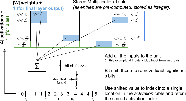
The second inefficiency is related to finding the activation function’s output value (or, more accurately, the index for that value in the LUT row space). Using the approach from Figure 8, finding the right output (one of ) requires that we examine the boundaries of the bins (). To address the inefficiency of needing to scan the boundaries, , in the activation function, we instead directly look-up the bin in the activation that contains the correct output (see Figure 9). After the summation of the inputs is computed, it is bit-shifted by bits, removing the least significant bits and giving the index of the bin in the activation table to look in. The binning (in the original activation-input space) is wide, which we have already accounted for by the scale factor that we included in our stored LUT values. So bit shifting by bits has replaced a linear (or binary) scan of the boundaries, giving a speed up relative to scanning (or, alternatively, relative to general multiplication and divide operations).
One of the limitations of this lookup-approach is that it works in cases in which the spacings between the activation boundaries are integer multiples of a uniform step size, . For the ReLU-6 activations, this is simple: the boundaries are spaced uniformly; and the activation table size is just entries.777In fact for ReLU6 with , the activation table can be completely omitted: it is just an identity mapping. However, when we quantize the tanh activation (Section 2.1), the width of the bins varies. For the example shown in Figures 8 and 9, the quantization boundaries are adjusted slightly from the “optimal” (that is, the boundary that would give the lowest quantization error relative to the original underlying tanh nonlinearity), so that we can set and have an activation table that is 12 entries long (pointing at 6 distinct quantized activation levels). In this case, the less we want to move our activation boundaries relative to the expected optimal, the smaller the value that must be and the larger that the activation table must be. Even so, since the table is a simple 1D array (in contrast with the multiplication table), the amount of memory that is needed for this table is negligible.
Since we are replacing floating point computations with table lookups and fixed-point summation, we need to guarantee that we will not overflow our underlying integer buffers. We are able to provide this guarantee by selecting appropriately. Our weights, one multiplicand, are always within a known, bounded range since we know our weight-cluster–center values. The previous layer’s outputs, the other multiplicand, are also in a known, bounded range since they are one of our quantization levels. Finally, by examining the network architecture, we know the maximum number of values that will need to be added by our summation step. If longer integers are required, this increase will only impact the buffer used by the summation (since that is the only location impacted by the maximum network fan-in). In the unlikely event that longer integers are required in the tables, this additional space is a minor expense in comparison to storing full resolution weights.
In summary, the final approach, shown in Figure 9, accomplishes what we set out to do at inference time: (1) eliminate multiplications in inference (2) eliminate floating point in inference and (3) eliminate computation of non-linearities without scanning of an activation input-to-output array.
Note that during training, floating point is used. Wu et al. (2018) addresses training with integers with various classification problems. Our goal is to ensure that networks, even if trained on the fastest GPUs, can be deployed on small devices that may be constrained in terms of power, speed or memory. Additionally, for our requirements, which encompass deployment of networks outside of the classification genre, we needed the quantization techniques to work with regression/real-valued outputs.
5 Discussion & Future Work
The need to enable more complex computations in the enormous number of deployed devices, rather than sending raw signals back to remote servers to be processed, is rapidly growing. For example, auditory processing within hearing aids, vision processing in remote sensors, custom signal processing in ASICs, or any of the recent photo applications running on the low and medium-powerful cell phones prevalent in many developing countries, all will benefit from on-device processing.
Pursuing quantized networks has led to a number of interesting questions for future exploration. Three immediate directions for future work are presented below. We also use this opportunity to discuss some of the insights/trends we noticed in our study but were not able to discuss fully here.
-
•
For quantizing weights, all of the network’s weights were placed into a single bucket. An alternative is to cluster the weights of each layer, or set of layers, independently. If there are distribution differences between layers (as can be seen in Figure 4), this may better capture the most significant weights from each layer. If this divided approach were used, there would be multiple multiplication tables stored for the same network. However, for large networks, the extra memory requirement would still be eclipsed by the saving of not representing each weight individually and the order in which the different LUT are accessed would be predictable (based on network architecture), making any L1 caching more effective.
-
•
Currently, is kept constant throughout training. However, we have witnessed instability in the beginning of training when is small. These spikes in the training loss dissipate as training progresses. Starting training with a larger-than-desired and gradually decreasing it may address the initial instability.
-
•
We, and other studies, have noticed the regularization-type effects of these methods. Additionally, we have noticed improved performance when other regularizers, such as Dropout, are not used. The use of these methods as regularizers is open for future work.
Beyond the practical ramifications of these simplified networks, perhaps what is most interesting are the implications of the simplified networks on network capacity. In general, we have embraced training ever larger networks to address growing task complexity and performance requirements. However, if we can obtain close performance using only a small fraction of the representational power in the activations and the weights then, with respect to our current models, much smaller networks could store the same information. Why does performance improve with larger networks? Perhaps the answer lies in the pairing of the network architectures and the learning algorithms. The learning algorithms control how the search through the weight-space progresses. It is likely that the architectures used today are explicitly optimized for the task and implicitly optimized for the learning algorithms employed. The large-capacity, widely-distributed, networks work well with the gradient descent algorithms used. Training networks to more efficiently store information, while maintaining performance, may require the use of alternate methods of exploring the weight-space.
References
- Agustsson et al. (2017) Agustsson, E., Mentzer, F., Tschannen, M., Cavigelli, L., Timofte, R., Benini, L., and Gool, L. V. Soft-to-hard vector quantization for end-to-end learned compression of images and neural networks. CoRR, abs/1704.00648, April 2017. URL http://arxiv.org/abs/1704.00648.
- Ballé et al. (2016) Ballé, J., Laparra, V., and Simoncelli, E. P. End-to-end optimized image compression. CoRR, abs/1611.01704, 2016. URL http://arxiv.org/abs/1611.01704.
- Baluja (2018) Baluja, S. Empirical explorations in training networks with discrete activations. CoRR, abs/1801.05156, January 2018. URL http://arxiv.org/abs/1801.05156.
- Bengio et al. (2013) Bengio, Y., Léonard, N., and Courville, A. C. Estimating or propagating gradients through stochastic neurons for conditional computation. CoRR, abs/1308.3432, August 2013. URL http://arxiv.org/abs/1308.3432.
- Bourzac (2017) Bourzac, K. Speck-size computers: Now with deep learning [news]. IEEE Spectrum, 54(4):13–15, April 2017.
- Cottrell & Munro (1988) Cottrell, G. W. and Munro, P. Principal components analysis of images via back propagation. In Visual Communications and Image Processing’88: Third in a Series, volume 1001, pp. 1070–1078. International Society for Optics and Photonics, October 1988.
- Courbariaux et al. (2016) Courbariaux, M., Hubara, I., Soudry, D., El-Yaniv, R., and Bengio, Y. Binarized neural networks: Training deep neural networks with weights and activations constrained to +1 or-1. arXiv preprint arXiv:1602.02830, February 2016.
- Deng et al. (2017) Deng, L., Jiao, P., Pei, J., Wu, Z., and Li, G. Gated XNOR networks: Deep neural networks with ternary weights and activations under a unified discretization framework. CoRR, abs/1705.09283, May 2017. URL http://arxiv.org/abs/1705.09283.
- Denton et al. (2014) Denton, E. L., Zaremba, W., Bruna, J., LeCun, Y., and Fergus, R. Exploiting linear structure within convolutional networks for efficient evaluation. In Ghahramani, Z., Welling, M., Cortes, C., Lawrence, N. D., and Weinberger, K. Q. (eds.), Advances in Neural Information Processing Systems 27, pp. 1269–1277. Curran Associates, Inc., December 2014.
- Duda et al. (1995) Duda, R. O., Hart, P. E., and Stork, D. G. Pattern classification and scene analysis 2nd ed. ed: Wiley Interscience, pp. 39–42, 1995.
- Finnerty & Ratigner (2017) Finnerty, A. and Ratigner, H. Reduce power and cost by converting from floating point to fixed point, March 2017. URL http://www.xilinx.com/support/documentation/white_papers/wp491-floating-to-fixed-point.pdf.
- Glorot et al. (2011) Glorot, X., Bordes, A., and Bengio, Y. Deep sparse rectifier neural networks. In Proceedings of the Fourteenth International Conference on Artificial Intelligence and Statistics, pp. 315–323, April 2011.
- Goodfellow et al. (2013) Goodfellow, I. J., Warde-Farley, D., Mirza, M., Courville, A., and Bengio, Y. Maxout networks. arXiv preprint arXiv:1302.4389, February 2013.
- Han et al. (2016) Han, S., Mao, H., and Dally, W. J. Deep compression: Compressing deep neural networks with pruning, trained quantization and huffman coding. International Conference on Learning Representations (ICLR), May 2016.
- Hinton (2012) Hinton, G. Neural networks for machine learning. Coursera, video lectures, 2012. URL https://www.coursera.org/learn/neural-networks.
- Hou et al. (2016) Hou, L., Yao, Q., and Kwok, J. T. Loss-aware binarization of deep networks. arXiv preprint arXiv:1611.01600, November 2016.
- Hubara et al. (2016) Hubara, I., Courbariaux, M., Soudry, D., El-Yaniv, R., and Bengio, Y. Quantized neural networks: Training neural networks with low precision weights and activations. arXiv arXiv:1609.07061, September 2016.
- Isola et al. (2016) Isola, P., Zhu, J.-Y., Zhou, T., and Efros, A. A. Image-to-image translation with conditional adversarial networks. arXiv preprint arXiv:1611.07004, November 2016.
- Jain (2010) Jain, A. K. Data clustering: 50 years beyond k-means. Pattern recognition letters, 31(8):651–666, August 2010.
- Jiang (1999) Jiang, J. Image compression with neural networks–a survey. Signal Processing: Image Communication, 14(9):737–760, 1999.
- Kingma & Ba (2015) Kingma, D. and Ba, J. Adam: A method for stochastic optimization. In International Conference on Learning Representations (ICLR), May 2015.
- Kohonen (1995) Kohonen, T. Learning vector quantization. In Self-Organizing Maps, pp. 175–189. Springer, 1995.
- Kramer (1991) Kramer, M. A. Nonlinear principal component analysis using autoassociative neural networks. AIChE journal, 37(2):233–243, February 1991.
- Krizhevsky & Hinton (2010) Krizhevsky, A. and Hinton, G. Convolutional deep belief networks on cifar-10. Unpublished manuscript, 40:7, 2010.
- Krizhevsky et al. (2012) Krizhevsky, A., Sutskever, I., and Hinton, G. E. Imagenet classification with deep convolutional neural networks. In Advances in neural information processing systems, pp. 1097–1105, 2012.
- Lane et al. (2015) Lane, N. D., Bhattacharya, S., Georgiev, P., Forlivesi, C., and Kawsar, F. An early resource characterization of deep learning on wearables, smartphones and internet-of-things devices. In Proceedings of the 2015 International Workshop on Internet of Things towards Applications, pp. 7–12. ACM, 2015.
- LeCun et al. (1998) LeCun, Y., Cortes, C., and Burges, C. J. The MNIST database of handwritten digits, 1998. URL http://yann.lecun.com/exdb/mnist/.
- Li et al. (2017) Li, H., De, S., Xu, Z., Studer, C., Samet, H., and Goldstein, T. Training quantized nets: A deeper understanding. In Neural Information Processing Systems, December 2017.
- Lin et al. (2015) Lin, D. D., Talathi, S. S., and Annapureddy, V. S. Fixed point quantization of deep convolutional networks. CoRR, abs/1511.06393, November 2015. URL http://arxiv.org/abs/1511.06393.
- Maddison et al. (2016) Maddison, C. J., Mnih, A., and Teh, Y. W. The concrete distribution: A continuous relaxation of discrete random variables. CoRR, abs/1611.00712, November 2016. URL http://arxiv.org/abs/1611.00712.
- Mentzer et al. (2018) Mentzer, F., Agustsson, E., Tschannen, M., Timofte, R., and Gool, L. V. Conditional probability models for deep image compression. CoRR, abs/1801.04260, January 2018. URL http://arxiv.org/abs/1801.04260.
- Nair & Hinton (2010) Nair, V. and Hinton, G. E. Rectified linear units improve restricted boltzmann machines. In Proceedings of the 27th international conference on machine learning (ICML), pp. 807–814, June 2010.
- Plagianakos et al. (2001) Plagianakos, V., Magoulas, G., Nousis, N., and Vrahatis, M. Training multilayer networks with discrete activation functions. In Neural Networks, 2001. Proceedings. IJCNN’01. International Joint Conference on, volume 4, pp. 2805–2810. IEEE, July 2001.
- Raiko et al. (2014) Raiko, T., Berglund, M., Alain, G., and Dinh, L. Techniques for learning binary stochastic feedforward neural networks. arXiv preprint arXiv:1406.2989, June 2014.
- Rastegari et al. (2016) Rastegari, M., Ordonez, V., Redmon, J., and Farhadi, A. XNOR-net: Imagenet classification using binary convolutional neural networks. In European Conference on Computer Vision, pp. 525–542. Springer, October 2016.
- Rippel & Bourdev (2017) Rippel, O. and Bourdev, L. Real-time adaptive image compression. arXiv preprint arXiv:1705.05823, 2017.
- Rumelhart et al. (1986) Rumelhart, D. E., Hinton, G. E., and Williams, R. J. Learning representations by back-propagating errors. nature, 323(6088):533, 1986.
- Russakovsky et al. (2014) Russakovsky, O., Deng, J., Su, H., Krause, J., Satheesh, S., Ma, S., Huang, Z., Karpathy, A., Khosla, A., Bernstein, M. S., Berg, A. C., and Li, F. Imagenet large scale visual recognition challenge. CoRR, abs/1409.0575, September 2014. URL http://arxiv.org/abs/1409.0575.
- Srivastava et al. (2014) Srivastava, N., Hinton, G. E., Krizhevsky, A., Sutskever, I., and Salakhutdinov, R. Dropout: a simple way to prevent neural networks from overfitting. Journal of machine learning research, 15(1):1929–1958, 2014.
- Svoboda et al. (2016) Svoboda, P., Hradis, M., Barina, D., and Zemcík, P. Compression artifacts removal using convolutional neural networks. CoRR, abs/1605.00366, May 2016. URL http://arxiv.org/abs/1605.00366.
- Tang & Salakhutdinov (2013) Tang, Y. and Salakhutdinov, R. R. Learning stochastic feedforward neural networks. In Advances in Neural Information Processing Systems, pp. 530–538, December 2013.
- Toderici et al. (2016) Toderici, G., O’Malley, S. M., Hwang, S. J., Vincent, D., Minnen, D., Baluja, S., Covell, M., and Sukthankar, R. Variable rate image compression with recurrent neural networks. In International Conference on Learning Representations, 2016.
- Toderici et al. (2017) Toderici, G., Vincent, D., Johnston, N., Hwang, S. J., Minnen, D., Shor, J., and Covell, M. Full resolution image compression with recurrent neural networks. In Computer Vision and Pattern Recognition (CVPR), 2017 IEEE Conference on, pp. 5435–5443. IEEE, 2017.
- Vanhoucke et al. (2011) Vanhoucke, V., Senior, A., and Mao, M. Z. Improving the speed of neural networks on CPUs. In Deep Learning and Unsupervised Feature Learning Workshop, NIPS 2011, December 2011.
- Werbos (1974) Werbos, P. Beyond regression: new tools for prediction and analysis in the behavioral sciences. PhD thesis, Harvard University, 1974.
- Wu et al. (2018) Wu, S., Li, G., Chen, F., and Shi, L. Training and inference with integers in deep neural networks. arXiv preprint arXiv:1802.04680, February 2018.
- Yi et al. (2008) Yi, Y., Hangping, Z., and Bin, Z. A new learning algorithm for neural networks with integer weights and quantized non-linear activation functions. In IFIP International Conference on Artificial Intelligence in Theory and Practice, pp. 427–431. Springer, 2008.
- Zhou et al. (2016) Zhou, S., Wu, Y., Ni, Z., Zhou, X., Wen, H., and Zou, Y. DoReFa-net: Training low bitwidth convolutional neural networks with low bitwidth gradients. arXiv arXiv:1606.06160, June 2016.