Toric Landau–Ginzburg models

Abstract.

This is a review of the theory of toric Landau–Ginzburg models — the effective approach to mirror symmetry for Fano varieties. We mainly focus on the cases of dimensions $2$ and $3$, as well as on the case of complete intersections in weighted projective spaces and Grassmannians. Conjectures that relate invariants of Fano varieties and their Landau–Ginzburg models, such as Katzarkov–Kontsevich–Pantev conjectures, are also studied.

Part I Introduction.

One of the most brilliant ideas in mathematics in the last three decades is Mirror Symmetry. As it often happens, it came to mathematics from physics. That is, Calabi–Yau threefolds (i. e. varieties of complex dimension $3$ with non-vanishing everywhere defined holomorphic $3$-form) play a central role in elementary particles description in the string theory. These varieties, enhanced by symplectic forms and complex structures, can be considered as symplectic or algebraic manifolds. Physicists noticed that these varieties come in (non-uniquely defined) pairs such that symplectic properties of Calabi–Yau manifold $X$ (the so called branes of type $A$) correspond to algebraic properties of its pair $Y$ (the so called branes of type $B$) and, vice-versa, symplectic properties for $Y$ correspond to algebraic properties for $X$. One of numerical consequences of the correspondence is Mirror Symmetry of Hodge numbers. It states that $h^{i,j}(X)=h^{i,3-j}(Y)$. One can say that putting a mirror to Hodge diamond for $X$ one can see the Hodge diamond for $Y$. This justifies the term ‘‘Mirror Symmetry’’.

Just after making this breakthrough it was straightforwardly generalized to higher-dimensional Calabi–Yau varieties. Some numerical consequences of the discovery were also formulated, which enabled one to formulate the idea of Mirror Symmetry mathematically. The first example of the phenomena is the famous paper [COGP91], where the generic quintic threefold in ${\mathbb{P}}^{4}$ was considered. The certain series for the hypersurface was considered, that is the one constructed by expected numbers of rational curves of given degree lying on the variety (Clemens conjecture states that for very generic quintic the numbers are finite). The certain one-dimensional family was considered. The period for the family, that is the function given by integrals of fiberwise forms over fiberwise cycles, after certain transformation coincides with the series for the quintic. This principle of correspondence of the series constructed by numbers of rational curves lying on the manifold and periods of the dual one-parameter family is the basement of the Mirror Symmetry conjecture of variations of Hodge structures.

The following generalization of Mirror Symmetry is the one for Fano varieties, that is varieties with ample anticanonical class. Such varieties play an important role in algebraic geometry: for instance, they are the main ‘‘building bricks’’ in Minimal Model Program. Moreover, they have rich geometry; say, a lot of rational curves lie on them. In opposite to the Calabi–Yau case, mirror partners for Fano varieties are not varieties of the same kind but certain varieties together with complex-valued functions called superpotential. Such varieties are called Landau–Ginzburg models and they can be described as one-dimensional families of fibers of superpotentials. In particular, fibers of the families are Calabi–Yau varieties mirror dual to anticanonical sections of the Fano varieties. Mirror Symmetry conjecture of variations of Hodge structures claims the correspondence between $I$-series that are constructed by Gromov–Witten invariants, that are expected numbers of rational curves of given degree lying on the manifold (it’s important here that it is Fano or close to be Fano to have enough rational curves) and periods of the dual family. In other words it claims the coincidence of the second Dubrovin’s connection for the Fano manifold and the Gauss–Manin connection for the dual Landau–Ginzburg model, or coincidence of regularized quantum differential equation of the variety and Picard–Fuchs differential equation of the dual model.

The first and the main example when Mirror Symmetry conjecture of variations of Hodge structures holds was given by Givental (see [Gi97b], and also [HV00])). He constructed Landau–Ginzburg models for complete intersections in smooth toric varieties. This construction can be generalized to complete intersections in singular toric varieties and, more general, varieties admitting ‘‘good’’ toric degenerations, such as Grassmannians or partial flag manifolds (see [BCFKS97] and [BCFKS98]). Moreover, Givental’s model for a toric variety $T$ can be simplified by expressing monomially some variables in terms of others such that the superpotential becomes a Laurent polynomial in $\dim(T)$ variables. The Newton polytope of the Laurent polynomial coincide with the fan polytope for $T$, that is a convex hull of integral generators of rays of a fan for $T$. For a complete intersection it is often possible to make one more birational change of variables after which the superpotential remains being representable by a Laurent polynomial. Moreover, this change of variables transforms Givental integral (that express periods) correctly.

Consider a Gorenstein toric variety $T$. Its fan polytope is reflexive, which means that the dual the polytope is integral. Consider the dual to $T$ toric variety $T^{\vee}$; in other words the varieties $T$ and $T^{\vee}$ are defined by dual polytopes. Let $X$ be a Calabi–Yau complete intersection in $T$ of dimension $n$, which is defined by some nef-partition. Batyrev and Borisov (see [BB96]) defined the dual nef-partition, which gives the dual Calabi–Yau variety $Y$. According to Givental, Mirror Symmetry conjecture of variations of Hodge structures holds for $X$ and $Y$. In loc. cit it is shown that

$$h_{st}^{p,q}(X)=h_{st}^{p,n-q}(Y),$$

where $h_{st}^{p,q}(Y)$ are stringy Hodge numbers. (In particular in our case they coincide with Hodge numbers of a crepant resolution of $Y$, which, by Batyrev’s theorem (see [Ba99]) do not depend on the particular resolution.) Thus in our case Mirror Symmetry conjecture for Hodge numbers follows from Mirror Symmetry conjecture of variations of Hodge structures. In the Fano case one can’t claim the correspondence of Hodge diamonds because the dual objects are not varieties but families of varieties. In [KKP17] the analogues of Hodge numbers for ‘‘tame compactified Landau–Ginzburg models’’ were defined (in three ways). The authors made a conjecture about mirror correspondence for them. We in particular study these conjectures in this paper, correct them a bit and observe schemes of their proofs for the two- and three-dimensional cases.

The next step is Kontsevich’s Homological Mirror Symmetry conjecture. It states mirror correspondence in terms of derived categories. That is, considering Fano manifold $X$ as an algebraic variety one can construct the derived category of coherent sheaves $D^{b}(coh\ X)$, and considering $X$ as a symplectic variety (with chosen symplectic form) one can construct the Fukaya category $Fuk(X)$, whose objects are Lagrangian submanifolds for the symplectic form, and morphisms are Floer homology. On the other hand, similar categories can be defined for a Landau–Ginzburg model $w\colon Y\to{\mathbb{C}}$. Analogue of the derived category of coherent sheaves for the Landau–Ginzburg model is the derived category of singularities $D^{b}_{sing}(Y,w)$, that is a product over all singular fibers of quotients of categories of coherent sheaves by subcategories of perfect complexes. Analogue of the Fukaya category is the Fukaya–Seidel category $FS(Y,w)$, whose objects are vanishing to singularities Lagrangian cycles (for chosen symplectic form on the Landau–Ginzburg model). Homological Mirror Symmetry conjecture states the equivalences

$$Fuk(X)\cong D^{b}_{sing}(Y,w),\ \ \ \ D^{b}(coh\ X)\cong FS(Y,w).$$

Homological Mirror Symmetry conjecture is very powerful. For instance, the Bondal–Orlov theorem states that a Fano variety can be reconstructed from its derived category of coherent sheaves. However because of the deepness of the conjecture it is hard to prove it even for the simplest cases. The positive examples are the partial proofs of the conjecture (that is, the proof of one of equivalences in the conjecture) for del Pezzo surfaces ([AKO06]), toric varieties ([Ab09]), and some of hypersurfaces ([Sh15]). Let us mention that Mirror Symmetry conjecture of variations of Hodge structures is claimed to be a numerical consequence of Homological Mirror Symmetry conjecture, since the equivalence of categories implies the isomorphism of their Hochschild cohomologies, which in our case correspond to quantum cohomology and variations of Hodge structures.

It is expected that different versions of mirror symmetry conjectures agree one with others. This means that Givental’s Landau–Ginzburg models satisfy Homological Mirror Symmetry conjecture. More precise, the following compactification principle should hold: there should exist fiberwise (log) compactification of a Landau–Ginzburg model which, after choosing a symplectic form, satisfies Homological Mirror Symmetry conjecture. In particular, fibers of the compactification should be Calabi–Yau varieties mirror dual to anticanonical sections of the Fano variety. These three properties (correspondence to Gromov–Witten invariants, the existence of compactification of a family of Calabi–Yau varieties, and a connection with toric degenerations) justify the notion of toric Landau–Ginzburg model which is central in this paper. Similarly to the case of smooth toric varieties (but not complete intersections therein!), toric Landau–Ginzburg model is an algebraic torus together with non-constant complex-valued function satisfying the properties discussed above. Since the function on the torus (after choosing a basis) is nothing but a Laurent polynomial, we call the Laurent polynomial (satisfying the properties) toric Landau–Ginzburg model. See Part III for the precise definition.

Strong version of Mirror Symmetry conjecture of variations of Hodge structures claims the existence of toric Landau–Ginzburg model for each smooth Fano variety.

The notion of toric Landau–Ginzburg model turned out to be an effective tool for studying mirror symmetry conjectures. This paper is a review of the theory of toric Landau–Ginzburg models. In particular, we construct them for a large class of Fano varieties such as del Pezzo surfaces, Fano threefolds, complete intersections in (weighted) projective spaces and Grassmannians. We also construct their compactifications and study their properties, invariants, and related conjectures.

We present only sketches of proofs for a lot of results in the paper; one can find details in the references. The paper is organized as follows. Part II contains definitions and preliminaries needed for the following. Part III is devoted to the notion of toric Landau–Ginzburg models. Del Pezzo surfaces are discussed in Part IV. We present there a precise construction of toric Landau–Ginzburg model depending on a divisor on a del Pezzo surface.

Part V, central in the paper, is devoted to the threefold case. Section V.1 contains construction of weak Landau–Ginzburg models. In Section V.2 (log) Calabi–Yau compactifications are constructed. In Section V.3 we discuss toric degenerations of Fano threefolds that correspond to their weak Landau–Ginzburg models. We also present a certain construction for the Picard rank one case. In Section V.4 we compute Picard lattices of fibers of Landau–Ginzburg models for the Picard rank one case and show that the fibers are Dolgachev–Nikulin mirrors to anticanonical sections of Fano varieties.

In Part VI we study Katzarkov–Kontsevich–Pantev conjectures on Hodge numbers of Landau–Ginzburg models. In Section VI we, following [KKP17], define and discuss Hodge numbers of Landau–Ginzburg models and Katzarkov–Kontsevich–Pantev conjectures. In Section VI.2 we prove the conjectures for del Pezzo surfaces. Finally, in Section VI.3 we present a scheme of the proof of the conjectures in the threefold case.

Part VII is devoted to the higher-dimensional case, that is the cases of (weighted) complete intersections and Grassmannians. A general Givental’s construction of Landau–Ginzburg models for complete intersections in smooth toric varieties is presented in Section VII.1. The most of results in the rest sections are related to the problem of existence of generalizations of such models and to the question if they are birational to weak Landau–Ginzburg models. In Section VII.2 we consider the case of weighted complete intersections. We present there results on existence of nef-partitions that guarantee the existence of weak Landau–Ginzburg models. In the case of complete intersections in the usual projective spaces we show existence of Calabi–Yau compactifications and toric degenerations. The rest of the section contains boundness results for families of smooth complete intersections. More details on this part one can find in the review [PSh18] (in preparation). Finally, in Section VII.3 we consider the case of complete intersections in Grassmannians. For each of such complete intersection we show the existence of Batyrev–Ciocan-Fontanine–Kim–van Straten construction which is birationally equivalent to weak Landau–Ginzburg models.

Notation and conventions

All varieties are considered over the field of complex numbers ${\mathbb{C}}$.

We consider only genus zero Gromov–Witten invariants.

Homology $H_{*}(X,{\mathbb{Z}})$ and cohomology $H^{*}(X,{\mathbb{Z}})$ we denote by $H_{*}(X)$ and $H^{*}(X)$ respectively. Cohomology with compact support (of a variety $X$ with coefficients in the constant sheaf ${\mathbb{C}}_{X}$) we denote by $H_{c}^{*}(X)$. Poincare dual class to $\gamma\in H^{*}(X)$ we denote by $\gamma^{\vee}$. The space $\mathrm{Pic}\,(X)\otimes{\mathbb{C}}$ we denote by $\mathrm{Pic}\,(X)_{\mathbb{C}}$.

For any two numbers $n_{1}$ and $n_{2}$ we denote the set $\{i\mid n_{1}\leqslant i\leqslant n_{2}\}$ by $[n_{1},n_{2}]$.

Calabi–Yau variety for us is a projective variety with trivial canonical class.

We often denote a Cartier divisor on a variety $X$ and its class in $\mathrm{Pic}\,(X)$ by the same symbol.

A smooth degree $d$ del Pezzo surface (except for the quadric surface) we denote by $S_{d}$.

A smooth Fano variety (considered as an element of a family of the varieties of its type) of Picard rank $k$ and number $m$ in the lists in [IP99] we denote by $X_{k-m}$.

We use the notation ${\mathbb{P}}(w_{0},\ldots,w_{n})$ for a weighted projective space with weights $w_{0},\ldots,w_{n}$. (Weighted) projective spaces with coordinates $x_{0},\ldots,x_{n}$ we denote by ${\mathbb{P}}[x_{0}:\ldots:x_{n}]$. Affine space with coordinates $x_{0},\ldots,x_{n}$ we denote by ${\mathbb{A}}[x_{1},\ldots,x_{n}]$.

The ring ${\mathbb{C}}[x_{1}^{\pm 1},\ldots,x_{n}^{\pm 1}]$ we denote by ${\mathbb{T}}[x_{1},\ldots,x_{n}]$. The torus $\mathrm{Spec}\,{\mathbb{T}}[x_{1},\ldots,x_{n}]$ we denote by $\mathcal{T}[x_{1},\ldots,x_{n}]$.

An integral polytope $\Delta\in{\mathbb{Z}}^{n}\otimes{\mathbb{R}}$ for us is a polytope with integral vertices, that is ones lying in ${\mathbb{Z}}^{n}$. An integral length of an integral segment is a number of integral points on it minus one.

We consider pencils in the birational sense. That is, a pencil for us is a family birational to a family of fibers of a map to ${\mathbb{P}}^{1}$.

Part II Preliminaries.

II.1. Gromov–Witten invariants and $I$-series

In this part we introduce notions and notation of Gromov–Witten theory we need. Details one can find, say, in [Ma99].

Definition II.1 ([Ma99, V–3.3.2]).

The moduli space of stable maps of rational curves of class $\beta\in H_{2}(X)$ with $n$ marked points to $X$ is the Deligne–Mumford stack (see [Ma99], V–5.5) of stable maps $f\colon C\to X$ of genus $0$ curves with $n$ marked points such that $f_{*}(C)=\beta$.

Consider the evaluation maps $ev_{i}:\bar{M}_{n}(X,\beta)\rightarrow X$, given by $ev_{i}(C;p_{1},\ldots,p_{n},f)=f(p_{i})$. Let $\pi_{n+1}:\bar{M}_{n+1}(X,\beta)\rightarrow\bar{M}_{n}(X,\beta)$ be the forgetful map at the point $p_{n+1}$ which forget this point and contract unstable component after it. Consider the sections

$$\sigma_{i}:\bar{M}_{n}(X,\beta)\rightarrow\bar{M}_{n+1}(X,\beta)$$

defined as follows. The image of a curve $(C;p_{1},\ldots,p_{n},f)$ under the map $\sigma_{i}$ is a curve $(C^{\prime};p_{1},\ldots,p_{n+1},f^{\prime})$. Here $C^{\prime}=C\bigcup C_{0}$, $C_{0}\simeq{\mathbb{P}}^{1}$, $C_{0}$ and $C$ intersect at the non-marked point $p_{i}$ on $C^{\prime}$, and $p_{n+1}$ and $p_{i}$ lie on $C_{0}$. The map $f^{\prime}$ contracts the curve $C_{0}$ to the point and $f^{\prime}|_{C}=f$.

Consider the sheaf $L_{i}$ given by $L_{i}=\sigma_{i}^{*}\omega_{\pi_{n+1}}$, where $\omega_{\pi_{n+1}}$ is a relative dualizing sheaf of $\pi_{n+1}$. Its fiber over the point $(C;p_{1},\ldots,p_{n},f)$ is $T^{*}_{p_{i}}C$.

Definition II.2 ([Ma99, VI–2.1]).

The cotangent line class is the class

$$\psi_{i}=c_{1}(L_{i})\in H^{2}(\bar{M}_{n}(X,\beta)).$$

Definition II.3 ([Ma99, VI–2.1]).

Consider

$$\gamma_{1},\ldots,\gamma_{n}\in H^{*}(X),$$

let $a_{1},\ldots,a_{n}$ be non-negative integers, and let $\beta\in H_{2}(X)$. Then the Gromov–Witten invariant with descendants is the number given by

$$\langle\tau_{a_{1}}\gamma_{1},\ldots,\tau_{a_{n}}\gamma_{n}\rangle_{\beta}=ev_{1}^{*}\gamma_{1}\cdot\psi_{1}^{a_{1}}\cdot\ldots\cdot ev_{n}^{*}\gamma_{n}\cdot\psi_{n}^{a_{n}}\cdot[\bar{M}_{n}(X,\beta)]^{\mathrm{virt}}$$

if $\sum\mathrm{codim}\,\gamma_{i}+\sum a_{i}=\mathrm{vdim}\,\bar{M}_{n}(X,\beta)$ and 0 otherwise. The invariants with $a_{i}=0$, $i=1\ldots,n$, are called prime. We omit symbols $\tau_{0}$ in this case.

Gromov–Witten invariants are usually ‘‘packed’’ into different structures for convenience. The simplest ones are one-pointed ($n=1$); they are usually packed to $I$-series.

Let $X$ be a smooth Fano variety of dimension $N$ and Picard number $\rho$. Choose a basis

$$\{H_{1},\ldots,H_{\rho}\}$$

in $H^{2}(X)$ so that for any $i\in[1,\rho]$ and any curve $\beta$ in the Kähler cone $K$ of $X$ one has $H_{i}\cdot\beta\geqslant 0$. Introduce formal variables $q^{\tau_{i}}$, $i\in[1,\rho]$ and denote $q_{i}=q^{\tau_{i}}$. For any $\beta\in H_{2}(X)$ denote

$$q^{\beta}=q^{\sum\tau_{i}(H_{i}\cdot\beta)}.$$

Consider the Novikov ring $\mathbb{C}_{q}$, i. e. a group ring for $H_{2}(X)$. We treat it as a ring of polynomials over $\mathbb{C}$ in formal variables $q^{\beta}$, with relations

$$q^{\beta_{1}}q^{\beta_{2}}=q^{\beta_{1}+\beta_{2}}.$$

Note that for any $\beta\in K$ the monomial $q^{\beta}$ has non-negative degrees in $q_{i}$.

Definition II.4 (details see in [Gat02], [Prz07a]).

Let $\mu_{1},\ldots,\mu_{N}$ be a basis in $H^{*}(X)$ and let $\check{\mu}_{1},\ldots,\check{\mu}_{N}$ be the dual basis. The $I$-series (or Givental $J$-series) for $X$ is given by the following.

$$I^{X}_{\beta}=ev_{*}\left(\frac{1}{1-\psi}\cdot[\bar{M}_{1}(X,\beta)]^{\mathrm{virt}}\right)=\sum_{i,j\geqslant 0}\langle\tau_{i}\mu_{j}\rangle_{\beta}\check{\mu}_{j},$$

$$I^{X}(q_{1},\ldots,q_{\rho})=1+\sum_{\beta\in K}I_{\beta}^{X}\cdot q^{\beta}.$$

The constant term of $I$-series $I^{X}_{0}$ is

$$I^{X}_{0}(q_{1},\ldots,q_{\rho})=1+\sum_{\beta\in K}\langle\tau_{(-K_{X})\cdot\beta-2}{\mathbf{1}}\rangle_{\beta}\cdot q^{\beta},$$

where $\mathbf{1}$ is the fundamental class. (The map $ev$ and the cotangent line class are unique for one-pointed invariants, so we omit indices.) The series

$$\widetilde{I}^{X}_{0}(q_{1},\ldots,q_{\rho})=1+\sum_{\beta\in K}(-K_{X}\cdot\beta)!\langle\tau_{-K_{X}\cdot\beta-2}\mathbf{1}\rangle_{\beta}\cdot q^{\beta}$$

is called the constant term of regularized $I$-series for $X$.

Consider the class of divisors $H=\sum\alpha_{i}H_{i}$. One can restrict $I$-series, the usual and the regularized ones, to the direction corresponding to the divisor class putting $\sigma_{i}=\alpha_{i}\sigma$ and $t=q^{\sigma}$. Let us fix a divisor class $D$. We are interesting in restrictions of $I$-series on the anticanonical direction corresponding to $D$. For this we change $q^{\beta}$ by $e^{-D\cdot\beta}t^{-K_{X}\cdot\beta}$. In particular one can define a restriction of the constant term of regularized $I$-series to the anticanonical direction (so that $D=0$). It has the form

$$\widetilde{I}^{X}_{0}(t)=1+a_{1}t+a_{2}t^{2}+\ldots,\ \ \ \ a_{i}\in{\mathbb{C}}.$$

II.2. Toric geometry

The definition and the main properties of toric varieties see in [Da78] or in [Fu93]. Let us just remind that toric variety is a variety with an action of a torus $\mathrm{Spec}\,({\mathbb{C}}^{*})^{N}$ such that one of its orbits is a Zariski open set. Toric variety is determined by its fan, i. e. some collection of cones with vertices in the points of lattice that is dual to the lattice of torus characters. Moreover, algebro-geometric properties of toric variety can be formulated in terms of properties of this fan. Remind some of them.

Every cone of the fan $\kappa\subset\mathcal{N}_{{\mathbb{R}}}=\mathcal{N}\otimes{\mathbb{R}}$, $\mathcal{N}\simeq{\mathbb{Z}}^{N}$ of dimension $r$ corresponds to the orbit of the torus of dimension $N-r$. Thus, each edge (one-dimensional cone) correspond to the (equivariant) Weil divisor. That is, let $\Sigma\in\mathcal{N}$ be a fan of the toric variety $X_{\Sigma}$ and let $\sigma\in\Sigma$ be any cone. Let $\mathcal{M}$ be a lattice dual to $\mathcal{N}$ with respect to some non-degenerate pairing $\langle\cdot,\cdot\rangle$ and $\sigma^{\vee}$ be a dual cone for $\sigma$ (i. e. $\sigma^{\vee}=\{l\in\mathcal{M}|\forall k\in\sigma\ \ \langle l,k\rangle\geqslant 0\}$). Let $U_{\sigma}=\mathrm{Spec}\,{\mathbb{C}}[\sigma^{\vee}]$ correspond to $\sigma$. The variety $X_{\sigma}$ is obtained from the affine varieties $U_{\sigma}$, $\sigma\in\Sigma$, by gluing together $U_{\sigma}$ and $U_{\tau}$ along $U_{\sigma\cap\tau}$, $\sigma,\tau\in\Sigma$. The divisors which correspond to the edges of the fan generate divisor class group. A Weil divisor $D=\sum d_{i}M_{i}$, where $M_{i}$ corresponds to edges, is Cartier if for each cone of the fan $\sigma$ there exist a vector $n_{\sigma}$ such that $\langle n_{\sigma},m_{i}\rangle=d_{i}$ where $m_{i}$ are primitive elements of the edges of this cone. If such vector is the same for all cones, then the divisor is principal. Hence if the toric variety is $N$-dimensional and the number of the edges is $N+\rho$, then the rank of the divisor class group is $\rho$.

Definition II.5.

The variety is called ${\mathbb{Q}}$-factorial if some multiple of each Weil divisor is a Cartier divisor.

In particular, there exists an intersection theory for Weil divisors on the ${\mathbb{Q}}$-factorial variety. Toric variety is ${\mathbb{Q}}$-factorial if and only if any cone of the fan, which corresponds to this variety, is simplicial. In this case the Picard group is generated (over ${\mathbb{Q}}$) by divisors, which correspond to the edges of the fan.

Consider a weighted projective space ${\mathbb{P}}={\mathbb{P}}(w_{0},\ldots,w_{N})$. The fan which corresponds to it is generated by integer vectors $m_{0},\ldots,m_{N}\in{\mathbb{R}}^{N}$ such that $\sum w_{i}m_{i}=0$. If $w_{0}=1$, then one can put $m_{0}=(-w_{1},\ldots,-w_{N})$, $m_{i}=e_{i}$, where $e_{i}$ is a basis of ${\mathbb{R}}^{N}$. The collection $\{m_{i}\}$ corresponds to the collection of standard divisors–strata $\{D_{i}\in H^{0}\left(\mathcal{O}_{\mathbb{P}}(w_{i})\right)\}$.

A toric variety is smooth if for any cone $\sigma$ in the fan that correspond to this variety the subgroup $\sigma\cap{\mathbb{Z}}^{N}$ is generated by the subset of the basis of the lattice $m_{1}^{\sigma},\ldots,m_{k}^{\sigma}$. Adding the edge $a=a_{1}m_{1}^{\sigma}+\ldots+a_{k}m_{k}^{\sigma}$, $a_{i}\in{\mathbb{Q}}$ to the cone (and connection it with ‘‘neighbor’’ faces) corresponds to weighted blow up (along subvariety which correspond to $\sigma$) with weights $1/r\cdot(\alpha_{1},\ldots,\alpha_{k})$, where $\alpha_{i}\in{\mathbb{Z}}$ and $a_{i}=\alpha_{i}/r$. Thus we can get toric resolution of a toric variety adding consecutively edges to the fan in this way.

In particular, singular locus of ${\mathbb{P}}$ is the union of strata given by $x_{i_{1}}=\ldots=x_{i_{j}}=0$, where $x_{i_{j}}$ is the coordinate of weight $w_{i_{j}}$ and $\{i_{1},\ldots,i_{j}\}$ is the maximal set of indices such that greatest common factor of the others is greater than $1$, see Lemma VII.18.

Let $X$ be a factorial $N$-dimensional toric Fano variety of Picard rank $\rho$ corresponding to a fan $\Sigma_{X}$ in the lattice $\mathcal{N}$. Let $D_{1},\ldots,D_{N+\rho}$ be its prime invariant divisors. Let $\mathcal{M}=\mathcal{N}^{\vee}$, and let $\mathcal{D}\simeq{\mathbb{Z}}^{N+\rho}$ be a lattice with the basis $\{D_{1},\ldots,D_{N+\rho}\}$ (so that one has a natural identification $\mathcal{D}\simeq\mathcal{D}^{\vee}$). By [CLS11, Theorem 4.2.1] one has an exact sequence

$$0\to\mathcal{M}\to\mathcal{D}\to A_{N-1}(X)=\mathrm{Pic}\,(X)\simeq{\mathbb{Z}}^{\rho}\to 0.$$

We use factoriality of $X$ here to identify the class group $A_{N-1}(X)$ and the Picard group $\mathrm{Pic}\,(X)$. Dualizing this exact sequence, we obtain an exact sequence

(II.6) $$0\to\mathrm{Pic}\,(X)^{\vee}\to\mathcal{D}\to\mathcal{N}\to 0.$$

Thus $\mathrm{Pic}\,(X)^{\vee}$ can be identified with the lattice of relations on primitive vectors on the rays of $\Sigma_{X}$ considered as Laurent monomials in variables $u_{i}$. On the other hand, as the basis in $\mathrm{Pic}\,(X)$ is chosen we can identify $\mathrm{Pic}\,(X)^{\vee}$ and $\mathrm{Pic}\,(X)=H^{2}(X)$. Hence we can choose a basis in the lattice of relations on primitive vectors on the rays of $\Sigma_{X}$ corresponding to $\{H_{i}\}$ and, thus, to $\{q_{i}\}$. We denote these relations by $R_{i}$, and interpret them as monomials in the variables $u_{1},\ldots,u_{N+\rho}$.

Consider a toric variety $T$. A fan (or spanning) polytope $F(T)$ is a convex hull of integral generators of fan’s rays for $T$. Let

$$\Delta=F(T)\subset\mathcal{N}_{\mathbb{R}}.$$

Let

$$\nabla=\{x\ |\ \langle x,y\rangle\geqslant-1\mbox{ for all }y\in\Delta\}\subset\mathcal{M}_{\mathbb{R}}=\mathcal{N}^{\vee}\otimes{\mathbb{R}}.$$

be the dual polytope.

For an integral polytope $\Delta$ we associate a (singular) toric Fano variety $T_{\Delta}$ defined by a fan whose cones are cones over faces of $\Delta$. We also associate a (not uniquely defined) toric variety $\widetilde{T}_{\Delta}$ with $F(\widetilde{T}_{\Delta})=\Delta$ such that for any toric variety $T^{\prime}$ with $F(T^{\prime})=\Delta$ and for any morphism $T^{\prime}\to\widetilde{T}_{\Delta}$ one has $T^{\prime}\simeq\widetilde{T}_{\Delta}$. In other words, $\widetilde{T}_{\Delta}$ is given by ‘‘maximal triangulation’’ of $\Delta$.

Definition II.7.

The variety $T_{\Delta}$ and the polytope $\Delta$ are called reflexive if $\nabla$ is integral.

Let $T$ be reflexive. Denote $T_{\nabla}$ by $T^{\vee}$ and $\widetilde{T}_{\nabla}$ by $\widetilde{T}^{\vee}$.

Finally summarize some facts related to toric varieties and their anticanonical sections. One can see, say, [Da78] for details. It is more convenient to start from the toric variety $T^{\vee}$ for the following.

Fact II.8.

Let the anticanonical class $-K_{T^{\vee}}$ be very ample (in particular, this holds in reflexive threefold case, see [JR06] and [CPS05]). One can embed $T^{\vee}$ to a projective space in the following way. Consider a set $A\subset M$ of integral points in a polytope $\Delta$ dual to $F(T^{\vee})$. Consider a projective space ${\mathbb{P}}$ whose coordinates $x_{i}$ correspond to elements $a_{i}$ of $A$. Associate a homogenous equation $\prod x_{i}^{\alpha_{i}}=\prod x_{j}^{\beta_{j}}$ with any homogenous relation $\sum\alpha_{i}a_{i}=\sum\beta_{j}a_{j}$, $\alpha_{i},\beta_{j}\in{\mathbb{Z}}_{+}$. The variety $T^{\vee}$ is cut out in ${\mathbb{P}}$ by equations associated to all homogenous relations on $a_{i}$.

Fact II.9.

The anticanonical linear system of $T^{\vee}$ is a restriction of $\mathcal{O}_{\mathbb{P}}(1)$. In particular, it can be described as (a projectivisation of) a linear system of Laurent polynomials whose Newton polytopes contain in $\Delta$.

Fact II.10.

Toric strata of $T^{\vee}$ of dimension $k$ correspond to $k$-dimensional faces of $\Delta$. Denote by $R_{f}$ an anticanonical section corresponding to a Laurent polynomial $f\in{\mathbb{C}}[N]$ and by $F_{Q}$ a stratum corresponding to a face $Q$ of $\Delta$. Denote by $f|_{Q}$ a sum of those monomials of $f$ whose support lie in $Q$. Denote by ${\mathbb{P}}_{Q}$ a projective space whose coordinates correspond to $Q\cap N$. (In particular, $Q$ is cut out in ${\mathbb{P}}_{Q}$ by homogenous relations on integral points of $Q\cap N$.) Then $R_{Q,f}=R_{f}|_{F_{Q}}=\{f|_{Q}=0\}\subset{\mathbb{P}}_{Q}$.

Fact II.11.

In particular, $R_{f}$ does not pass through a toric point corresponding to a vertex of $\Delta$ if and only if its coefficient at this vertex is non-zero. The constant Laurent polynomial corresponds to the boundary divisor of $T^{\vee}$.

Part III Toric Landau–Ginzburg models

Consider a smooth Fano manifold $X$ of dimension $n$ and a divisor $D$ on it. Consider the restriction

$$\widetilde{I}^{X,D}_{0}(t)=1+\sum_{\beta\in K,\ a\in{\mathbb{Z}}_{\geqslant 0}}(-K_{X}\beta)!\langle\tau_{a}\mathbf{1}\rangle_{\beta}\cdot e^{-\beta\cdot D}t^{-K_{X}\cdot\beta}$$

of constant term of regularized $I$-series corresponding to $D$.

Consider the torus $G_{\mathrm{m}}^{n}=\prod_{i=1}^{n}\mathcal{T}[x_{i}]$ and a function $f$ on it. This function can be represented by a Laurent polynomial: $f=f(x_{1}^{\pm 1}\ldots,x_{n}^{\pm 1})$. Denote the constant term (that is a coefficient at $x_{1}^{0}\cdot\ldots\cdot x_{n}^{0}$) of the polynomial $f$ by $[f]_{0}$ and put

$$\Phi_{f}=\sum_{i=0}^{\infty}[f^{i}]_{0}t^{i}\in{\mathbb{C}}[[t]].$$

Definition III.1.

The series $\Phi_{f}$ is called the constant terms series for $f$.

Definition III.2.

let $f$ be a Laurent polynomial in $n$ variables $x_{1},\ldots,x_{n}$. The integral

$$I_{f}(t)=\frac{1}{(2\pi i)^{n}}\int\limits_{|x_{i}|=\varepsilon_{i}}\frac{dx_{1}}{x_{1}}\wedge\ldots\wedge\frac{dx_{n}}{x_{n}}\frac{1}{1-tf}=\\ =\frac{1}{(2\pi i)^{n}}\sum_{j=0}^{\infty}t^{j}\cdot\int\limits_{|x_{i}|=\varepsilon_{i}}f^{j}\frac{dx_{1}}{x_{1}}\wedge\ldots\wedge\frac{dx_{n}}{x_{n}}\in{\mathbb{C}}[[t]]$$

is called the main period for $f$, where $\varepsilon_{i}$ are some positive real numbers.

Remark III.3.

One has $I_{f}(t)=\Phi_{f}$.

The following theorem justifies this definition.

Theorem III.4 (see [Prz08b, Proposition 2.3]).

Let $f$ be a Laurent polynomial in $n$ variables. Let $PF_{f}=PF_{f}\left(t,\frac{\partial}{\partial t}\right)$ be a Picard–Fuchs differential operator of the pencil of hypersurfaces in torus given by $f$. Then $PF_{f}[I_{f}(t)]=0$.

Now let us give the central definition of the paper.

Definition III.5 (see [Prz13, §6]).

A toric Landau–Ginzburg model for a pair of a smooth Fano variety $X$ of dimension $n$ and divisor $D$ on it is a Laurent polynomial $f\in{\mathbb{T}}[x_{1},\ldots,x_{n}]$ which satisfies the following.

Period condition:

One has $I_{f}=\widetilde{I}^{X,D}_{0}$.

Calabi–Yau condition:

There exists a relative compactification of a family

$$f\colon({\mathbb{C}}^{*})^{n}\to{\mathbb{C}}$$

whose total space is a (non-compact) smooth Calabi–Yau variety $Y$. Such compactification is called a Calabi–Yau compactification.

Toric condition:

There is a degeneration $X\rightsquigarrow T_{X}$ to a toric variety $T_{X}$ such that $F(T_{X})=N(f)$, where $N(f)$ is the Newton polytope for $f$.

Laurent polynomial satisfying the period condition is called a weak Landau–Ginzburg model.

Definition III.6 ([Prz17]).

A compactification of the family $f\colon({\mathbb{C}}^{*})^{n}\to{\mathbb{C}}$ to a family $f\colon Z\to{\mathbb{P}}^{1}$, where $Z$ is smooth and $-K_{Z}=f^{-1}(\infty)$, is called a log Calabi–Yau compactification (cf. Definition VI.3).

Now discuss why the notion of toric Landau–Ginzburg model is natural.

The period condition is nothing but Mirror Symmetry conjecture of variations of Hodge structures for the case when the ambient space is an algebraic torus. This condition relates Gromov–Witten invariants with periods of the dual model. Periods are integrals of fiberwise forms over fiberwise fibers. This means that they preserve under birational transformations which are biregular in the neighborhood of the cycles we integrating over. For instance, Givental constructed Landau–Ginzburg models in smooth toric varieties as quasi-affine varieties with superpotentials (see Section VII.1 and Paragraph VII.3.1). However in a lot of cases these models are birational to algebraic tori, and the main periods preserve under the corresponding birational isomorphisms, see Paragraph VII.2.2, Part VII and [DH15] and [CoKaPr14].

The Calabi–Yau condition is going back to the following principle.

Principle III.7 (Compactification principle, [Prz13, Principle 32]).

There exists a fiberwise compactification of family of fibers of ‘‘good’’ toric Landau–Ginzburg model (defined up to flops) satisfying (B side of) Homological Mirror Symmetry conjecture.

In particular this means that there should exist a fiberwise compactification to (open) smooth Calabi–Yau variety which is a family of smooth compact Calabi–Yau varieties. This condition is strong enough: say, if $f(x_{1},\ldots,x_{n})$ is a toric Landau–Ginzburg model for a variety $X$, then for $k>1$ the Laurent polynomial $f(x_{1}^{k},\ldots,x_{n})$ satisfies the period condition for $X$, but not the the Calabi–Yau condition and, thus, it does not satisfy the compactification principle.

Example III.8.

The polynomials

$$\frac{(x+y+1)^{3}}{xyzw}+z+w$$

and

$$\left(x_{1}+x_{2}+\frac{1}{x_{1}x_{2}}\right)\left(y_{1}+y_{2}+\frac{1}{y_{1}y_{2}}\right)$$

satisfy the period and Calabi–Yau conditions for a cubic fourfold (see [KP09]). However they are not fiberwise birational (they have different numbers of components of central fibers, cf. Section V.4). It is expected that the first polynomial satisfy the compactification principle.

One can easily see that the second Laurent polynomial in Example III.8 is not toric Landau–Ginzburg model for a cubic fourfold: the degree of the corresponding toric variety differs from the degree of cubic.

Finally, the toric condition goes back to Batyrev–Borisov construction of mirror duality for Calabi–Yau complete intersections in toric varieties via the duality of toric varieties, see [Ba93].

We consider mirror symmetry as a correspondence between Fano varieties and Laurent polynomials. That is, the strong version of Mirror Symmetry conjecture of variations of Hodge structures states the following.

Conjecture III.9.

Any pair of a smooth Fano manifold and a divisor on it has a toric Landau–Ginzburg model.

Corollary III.10.

Any smooth Fano variety has a toric degeneration.

This lets to hope to have the following picture.

Optimistic picture III.11 ([Prz13, Optimistic Picture 38]).

Toric degenerations of smooth Fano varieties are in one-to-one correspondence with toric Landau–Ginzburg models. They satisfy the compactification principle.

Question III.12.

Does the opposite to the second part of the compactification principle hold? That is, is it true that all Landau–Ginzburg models (in the sense of Homological Mirror Symmetry) of the same dimension as the initial Fano variety are compactifications of toric ones? In particular, is it true that all of them are rational?

Question III.13.

Does the Optimistic Picture III.11 need any extra condition on toric varieties?

Part IV Del Pezzo surfaces

We start the section by recalling well known facts about del Pezzo surfaces. We refer, say, to [Do12] as to one of huge amount of references on del Pezzo surfaces.

The initial definition of del Pezzo surface is the following one given by P. del Pezzo himself.

Definition IV.1 ([dP87]).

A del Pezzo surface is a non-degenerate (that is not lying in a linear subspace) irreducible linear normal (that is it is not a projection of degree $d$ surface in ${\mathbb{P}}^{d+1}$) surface in ${\mathbb{P}}^{d}$ of degree $d$ which is not a cone.

In modern words this means that a del Pezzo surface is an (anticanonically embedded) surface with ample anticanonical class and canonical (the same as du Val, simple surface, Kleinian, or rational double point) singularities. (Classes of canonical and Gorenstein singularities for surfaces coincide.) So we use the following more general definition.

Definition IV.2.

A del Pezzo surface is a complete surface with ample anticanonical class and canonical singularities. A weak del Pezzo surface is a complete surface with nef and big anticanonical class and canonical singularities.

Remark IV.3.

Weak del Pezzo surfaces are (partial) minimal resolutions of singularities of del Pezzo surfaces. Exceptional divisors of the resolutions are $(-2)$-curves.

A degree of del Pezzo surface $S$ is the number $d=(-K_{S})^{2}$. One has $1\leqslant d\leqslant 9$. If $d>2$, then the anticanonical class of $S$ is very ample and it gives the embedding $S\hookrightarrow{\mathbb{P}}^{d}$, so both definitions coincide. In this section we assume that $d>2$.

Obviously, projecting a degree $d$ surface in ${\mathbb{P}}^{d}$ from a smooth point on it one gets degree $d-1$ surface in ${\mathbb{P}}^{d-1}$. This projection is nothing but blow up of the center of the projection and blow down all lines passing through the point. (By adjunction formula these lines are $(-2)$-curves.) If we choose general (say, not lying on lines) centers of projections we get a classical description of a smooth del Pezzo surface of degree $d$ as a quadric surface (with $d=8$) or a blow up of ${\mathbb{P}}^{2}$ in $9-d$ points. They degenerate to singular surfaces which are projections from non-general points (including infinitely close ones). Moreover, all del Pezzo surfaces of given degree lie in the same irreducible deformation space except for degree $8$ when there are two components (one for a quadric surface and one for a blow up ${\mathbb{F}}_{1}$ of ${\mathbb{P}}^{2}$). General elements of the families are smooth, and all singular del Pezzo surfaces are degenerations of smooth ones in these families. This description enables us to construct toric degenerations of del Pezzo surfaces. That is, ${\mathbb{P}}^{2}$ is toric itself. Projecting from toric points one gets a (possibly singular) toric del Pezzo surfaces.

Remark IV.4.

The approach to description of del Pezzo surfaces via their toric degenerations and the connection of the degenerations by elementary transformations (projections) can be generalized to the threefold case. That is, smooth Fano threefolds can be connected via toric degenerations and toric basic links. For details see [ChKaPr13].

Remark IV.5.

Del Pezzo surfaces of degree $1$ or $2$ also have toric degenerations. Indeed, these surfaces can be described as hypersurfaces in weighted projective spaces, that is ones of degree $4$ in ${\mathbb{P}}(1,1,1,2)$ and of degree $6$ in ${\mathbb{P}}(1,1,2,3)$ correspondingly, so they can be degenerated to binomial hypersurfaces, cf. Example VII.36. However their singularities are worse then canonical.

Let $T_{S}$ be a Gorenstein toric degeneration of a del Pezzo surface $S$ of degree $d$. Let $\Delta=F(T_{S})\subset\mathcal{N}_{\mathbb{R}}={\mathbb{Z}}^{2}\otimes{\mathbb{R}}$ be a fan polygon of $T_{S}$. Let $f$ be a Laurent polynomial such that $N(f)=\Delta$.

Our goal now is to describe in details a way to construct a Calabi–Yau compactification for $f$. More precise, we construct a commutative diagram

where $Y$ and $Z$ are smooth, fibers of maps $Y\to{\mathbb{A}}^{1}$ and $Z\to{\mathbb{P}}^{1}$ are compact, and $-K_{Z}=f^{-1}(\infty)$; we denote all ‘‘vertical’’ maps in the diagram by $f$ for simplicity.

The strategy is the following. First we consider a natural compactification of the pencil $\{f=\lambda\}$ to an elliptic pencil in a toric del Pezzo surface $T^{\vee}$. Then we resolve singularities of $T^{\vee}$ and get a pencil in a smooth toric weak del Pezzo surface $\widetilde{T}^{\vee}$. Finally we resolve a base locus of the pencil to get $Z$. We get $Y$ cutting out strict transform of the boundary divisor of $\widetilde{T}^{\vee}$.

The polygon $\Delta$ has integral vertices in $\mathcal{N}_{\mathbb{R}}$ and it has the origin as a unique strictly internal integral point. A dual polygon $\nabla=\Delta^{\vee}\subset\mathcal{M}=\mathcal{N}^{\vee}$ has integral vertices and a unique strictly internal integral point as well. Geometrically this means that singularities of $T$ and $T^{\vee}$ are canonical.

Remark IV.6.

The normalized volume of $\nabla$ is given by

$$\mathrm{vol}\,\nabla=|\mbox{integral points in $\nabla$}|-1=(-K_{S})^{2}=d.$$

It is easy to see that

$$|\mbox{integral points on the boundary of $\Delta$}|+|\mbox{integral points on the boundary of $\nabla$}|=12.$$

In particular, $\mathrm{vol}\,\Delta=12-d$.

Compactification construction IV.7 ([Prz17]).

By Fact II.9, the anticanonical linear system on $T^{\vee}$ can be described as a projectivisation of a linear space of Laurent polynomials whose Newton polygons are contained in $\nabla^{\vee}=\Delta$. Thus the natural way to compactify the family is to do it using embedding $({\mathbb{C}}^{*})^{2}\hookrightarrow T^{\vee}$. Fibers of the family are anticanonical divisors in this (possibly singular) toric variety. Two anticanonical sections intersect by $(-K_{T^{\vee}})^{2}=\mathrm{vol}\,\Delta=12-d$ points (counted with multiplicities), so the compactification of the pencil in $T^{\vee}$ has $12-d$ base points (possibly with multiplicities). The pencil $\{\lambda_{0}f=\lambda_{1}\}$, $(\lambda_{0}:\lambda_{1})\in{\mathbb{P}}$, is generated by its general member and a divisor corresponding to a constant Laurent polynomial, i. e. to the boundary divisor of $T^{\vee}$. Let us mention that the torus invariant points of $T^{\vee}$ do not lie in the base locus of the family by Fact II.11.

Let $\widetilde{T}^{\vee}\to T^{\vee}$ be a minimal resolution of singularities of $T^{\vee}$. Pull back the pencil under consideration. We get an elliptic pencil with $12-d$ base points (with multiplicities), which are smooth points of the boundary divisor $D$ of the toric surface $\widetilde{T}^{\vee}$; this divisor is a wheel of $d$ smooth rational curves. Blow up these base points and get an elliptic surface $Z$. Let $E_{1},\ldots,E_{12-d}$ be the exceptional curves of the blow up $\pi\colon Z\to\widetilde{T}^{\vee}$; in particular, $Z$ is not toric. Denote a strict transform of $D$ by $D$ for simplicity. Then one has

$$-K_{Z}=\pi^{*}(-K_{\widetilde{T}^{\vee}})-\sum E_{i}=D+\sum E_{i}-\sum E_{i}=D.$$

Thus the anticanonical class $-K_{Z}$ contains $D$ and consists of fibers of $Z$. This, in particular, means that an open variety $Y=Z\setminus D$ is a Calabi–Yau compactification of the pencil provided by $f$. This variety has $e>0$ sections, where $e$ is a number of base points of the pencil in $\widetilde{T}^{\vee}$ counted without multiplicities.

Summarizing, we obtain an elliptic surface $f\colon Z\to{\mathbb{P}}^{1}$ with smooth total space $Z$ and a wheel $D$ of $d$ smooth rational curves over $\infty$.

Remark IV.8.

Let the polynomial $f$ be general among ones with the same Newton polygon. Then singular fibers of $Z\to{\mathbb{P}}^{1}$ are either curves with a single node or a wheel of $d$ rational curves over $\infty$. By Noether formula one has

$$12\chi(\mathcal{O}_{Z})=(-K_{Z})^{2}+e(Z)=e(Z),$$

where $e(Z)$ is a topological Euler characteristic. Thus singular fibers for $Z\to{\mathbb{P}}^{1}$ are $d$ curves with one node and a wheel of $d$ curves over $\infty$. This description is given in [AKO06].

Remark IV.9.

One can compactify all toric Landau–Ginzburg models for all del Pezzo surfaces of degree at least three simultaneously. That is, all reflexive polygons are contained in the biggest polygon $B$, that has vertices $(2,-1)$, $(-1,2)$, $(-1,-1)$. Thus fibers of all toric Landau–Ginzburg models can be simultaneously compactified to (possibly singular) anticanonical curves on $T_{B^{\vee}}={\mathbb{P}}^{2}$. Blow up the base locus to construct a base points free family. However in this case a general member of the family can pass through toric points as it can happen that $N(f)\varsubsetneq B$. This means that some of exceptional divisors of the minimal resolution are extra curves in a wheel over infinity.

In other words, consider a triangle of lines on ${\mathbb{P}}^{2}$. A general member of the pencil given by $f$ is an elliptic curve on ${\mathbb{P}}^{2}$. The total space of the log Calabi–Yau compactification is a blow up of nine intersection points (counted with multiplicities) of the elliptic curve and the triangle of lines. Exceptional divisors for points lying over vertices of the triangle are components of the wheel over infinity for the log Calabi–Yau compactification; the others are either sections of the pencil or components of fibers over finite points.

Now following [Prz17] describe toric Landau–Ginzburg models for del Pezzo surfaces and toric weak del Pezzo surfaces. That is, for a del Pezzo surface $S$, its Gorenstein toric degeneration $T$ with a fan polygon $\Delta$, its crepant resolution $\widetilde{T}$ with the same fan polygon, and a divisor $D\in\mathrm{Pic}\,(S)_{\mathbb{C}}\simeq\mathrm{Pic}\,(\widetilde{T})_{\mathbb{C}}$, we construct two Laurent polynomials $f_{S,D}$ and $f_{\widetilde{T},D}$, that are toric Landau–Ginzburg models for $S$ and $\widetilde{T}$ correspondingly, by induction. For this use, in particular, Givental’s construction of Landau–Ginzburg models for smooth toric varieties, see Section VII.1.

Let $S\simeq{\mathbb{P}}^{1}\times{\mathbb{P}}^{1}$ be a quadric surface, and let $D_{S}$ be an $(a,b)$-divisor on it. Let $T_{1}=S$, and let $T_{2}$ be a quadratic cone; $T_{1}$ and $T_{2}$ are the only Gorenstein toric degenerations of $S$. The crepant resolution of $T_{2}$ is a Hirzebruch surface ${\mathbb{F}}_{2}$, so let $D_{{\mathbb{F}}_{2}}=\alpha s+\beta f$, where $s$ is a section of ${\mathbb{F}}_{2}$, so that $s^{2}=-2$, and $f$ is a fiber of the map ${\mathbb{F}}_{2}\to{\mathbb{P}}^{1}$. Define

$$f_{S,D_{S}}=f_{\widetilde{T}_{1},D_{S}}=x+\frac{e^{-a}}{x}+y+\frac{e^{-b}}{y}$$

for the first toric degeneration and

$$f_{S,D_{S}}=y+e^{-a}\frac{1}{xy}+\left(e^{-a}+e^{-b}\right)\frac{1}{y}+e^{-b}\frac{x}{y},\ \ f_{\widetilde{T}_{2},D_{{\mathbb{F}}_{2}}}=y+\frac{e^{-\beta}}{xy}+\frac{e^{-\alpha}}{y}+\frac{x}{y}$$

for the second one.

Now assume that $S$ is a blow up of ${\mathbb{P}}^{2}$. First let $S=T=\widetilde{T}={\mathbb{P}}^{2}$, let $l$ be a class of a line on $S$, and let $D=a_{0}l$. Then up to a toric change of variables one has

$$f_{{\mathbb{P}}^{2},D}=x+y+\frac{e^{-a_{0}}}{xy}.$$

Now let $S^{\prime}$ be a blow up of ${\mathbb{P}}^{2}$ in $k$ points with exceptional divisors $e_{1},\ldots,e_{k}$, let $S$ be a blow up of $S^{\prime}$ in a point, and let $e_{k+1}$ be an exceptional divisor for the blow up. We identify divisors on $S^{\prime}$ and their strict transforms on $S$, so $\mathrm{Pic}\,(S^{\prime})=\mathrm{Pic}\,(\widetilde{T}^{\prime})={\mathbb{Z}}l+{\mathbb{Z}}{e_{1}}+\ldots+{\mathbb{Z}}{e_{k}}$ and $\mathrm{Pic}\,(S)={\mathbb{Z}}l+{\mathbb{Z}}{e_{1}}+\ldots+{\mathbb{Z}}{e_{k}}+{\mathbb{Z}}{e_{k+1}}$. Let $D^{\prime}=a_{0}l+a_{1}e_{1}+\ldots+a_{k}e_{k}\in\mathrm{Pic}\,(S^{\prime})_{\mathbb{C}}$ and $D=D^{\prime}+a_{k+1}e_{k+1}\in\mathrm{Pic}\,(S)_{\mathbb{C}}$. First describe the polynomial $f_{\widetilde{T},D}$. Combinatorially $\Delta=F(\widetilde{T})$ is obtained from a polygon $\Delta^{\prime}=F(\widetilde{T}^{\prime})$ by adding one integral point $K$ that corresponds to the exceptional divisor $e_{k+1}$, and taking a convex hull. Let $L$, $R$ be boundary points of $\Delta$ neighbor to $K$, left and right with respect to the clockwise order. Let $c_{L}$ and $c_{R}$ be coefficients in $f_{\widetilde{T}^{\prime},D^{\prime}}$ at monomials corresponding to $L$ and $R$. Let $M\in{\mathbb{T}}[x,y]$ be a monomial corresponding to $K$. Then from Givental’s description of Landau–Ginzburg models for toric varieties (see Section VII.1) one gets

$$f_{\widetilde{T},D}=f_{\widetilde{S}^{\prime},D^{\prime}}+c_{L}c_{R}e^{-a_{k+1}}M.$$

The polynomial $f_{S,D}$ differs from $f_{\widetilde{T},D}$ by coefficients at non-vertex boundary points. For any boundary point $K\in\Delta$ define marking $m_{K}$ as a coefficient of $f_{\widetilde{T},D}$ at $K$. Consider a facet of $\Delta$ and let $K_{0},\ldots,K_{r}$ be integral points in clockwise order of this facet. Then coefficient of $f_{S,D}$ at $K_{i}$ is a coefficient at $s^{i}$ in the polynomial

$$m_{K_{0}}\left(1+\frac{m_{K_{1}}}{m_{K_{0}}}s\right)\cdot\ldots\cdot\left(1+\frac{m_{K_{r}}}{m_{K_{r-1}}}s\right).$$

Remark IV.10.

One has $\mathrm{Pic}\,(S)\simeq\mathrm{Pic}\,(\widetilde{T})$. That is, if $S$ is not a quadric, then both $S$ and $\widetilde{T}$ are obtained by a sequence of blow ups in points (the only difference is that the points for $\widetilde{T}$ can lie on exceptional divisors of previous blow ups). Thus in both cases Picard groups are generated by a class of a line on ${\mathbb{P}}^{2}$ and exceptional divisors $e_{1},\ldots,e_{k}$. However an image of $e_{i}$ under the map of Picard groups given by the degeneration of $S$ to $\widetilde{T}$ can be not equal to $e_{i}$ itself but to some linear combination of the exceptional divisors. In other words these bases do not agree with degenerations.

Remark IV.11.

The spaces parameterizing toric Landau–Ginzburg models for $S$ and for $\widetilde{T}$ are the same — they are the spaces of Laurent polynomials with Newton polygon $\Delta$ modulo toric rescaling. Thus any Laurent polynomial corresponds to different elements of $\mathrm{Pic}\,(S)_{\mathbb{C}}\simeq\mathrm{Pic}\,(\widetilde{T})_{\mathbb{C}}$. This gives a map $\mathrm{Pic}\,(S)_{{\mathbb{C}}}\to\mathrm{Pic}\,(\widetilde{T})_{{\mathbb{C}}}$. However this map is transcendental because of exponential nature of the parametrization.

Proposition IV.12 ([Prz17, Proposition 21]).

The Laurent polynomial $f_{S,D}$ is a toric Landau–Ginzburg model for $(S,D)$.

Proof.

It is well known that $S$ is either a smooth toric variety or a complete intersection in a smooth toric variety. This enables one to compute a series $\widetilde{I}^{S}$ and, since, $\widetilde{I}^{S,D}$ following [Gi97b], see Theorem VII.11. Using this it is straightforward to check that the period condition for $f_{S,D}$ holds. The Calabi–Yau condition holds by Compactification Construction IV.7. Finally the toric condition holds by construction. (See Example IV.15.) ∎

Proposition IV.13 ([Prz17, Proposition 22]).

Consider two different Gorenstein toric degenerations $T_{1}$ and $T_{2}$ of a del Pezzo surface $S$. Let $\Delta_{1}=F(T_{1})$ and $\Delta_{2}=F(T_{2})$. Consider families of Calabi–Yau compactifications of Laurent polynomials with Newton polygons $\Delta_{1}$ and $\Delta_{2}$. Then there is a birational isomorphism of these families. In other words, there is a birational isomorphism between affine spaces of Laurent polynomials with supports in $\Delta_{1}$ and $\Delta_{2}$ modulo toric change of variables that preserves Calabi–Yau compactifications.

Proof.

One can check that polygons $\Delta_{1}$ and $\Delta_{2}$ differ by (a sequence of) mutations (see, say, [ACGK12]). These mutations agree with fiberwise birational isomorphisms of toric Landau–Ginzburg models modulo change of basis in $H^{2}(S,{\mathbb{Z}})$ by the construction. The statement follows from the fact that birational elliptic curves are isomorphic. ∎

Remark IV.14.

Let $D=0$. Then the polynomial $f_{S,0}$ has coefficients $1$ at vertices of its Newton polygon and $\binom{n}{k}$ at $k$-th integral point of an edge of integral length $n$. In other words, $f_{S,0}$ is binomial, cf. Section V.1.

Example IV.15.

Let $S=S_{7}$. This surface has two Gorenstein toric degenerations: it is toric itself, and also it can be degenerated to a singular surface which is obtained by a blow up of ${\mathbb{P}}^{2}$, a blow up of a point on the exceptional curve, and a blow down the first exceptional curve to a point of type $\mathbb{A}_{1}$.

Let $\Delta_{1}$ be the polygon with vertices $(1,0)$, $(1,1)$, $(0,1)$, $(-1,-1)$, $(0,-1)$, and let $D=a_{0}l+a_{1}e_{1}+a_{2}e_{2}$. Then

$$f_{\widetilde{T}_{\Delta_{1}},D}=f_{S,D}=x+y+e^{-a_{0}}\frac{1}{xy}+e^{-(a_{0}+a_{1})}\frac{1}{y}+e^{-a_{2}}xy.$$

Let $\Delta_{2}$ be the polygon with vertices $(1,0)$, $(0,1)$, $(-1,-1)$, and $(1,-1)$, and let $D=a_{0}l+a_{1}e_{1}+a_{2}e_{2}$. Then

$$f_{\widetilde{T}_{\Delta_{2}},D}=x+y+e^{-a_{0}}\frac{1}{xy}+e^{-(a_{0}+a_{1})}\frac{1}{y}+e^{-(a_{0}+a_{1}+a_{2})}\frac{x}{y},$$

$$f^{\prime}_{S,D}=x+y+e^{-a_{0}}\frac{1}{xy}+\left(e^{-(a_{0}+a_{1})}+e^{-(a_{0}+a_{2})}\right)\frac{1}{y}+e^{-(a_{0}+a_{1}+a_{2})}\frac{x}{y}.$$

(Here $f_{S,D}$ and $f^{\prime}_{S,D}$ are toric Landau–Ginzburg models for $(S,D)$ in different bases in $({\mathbb{C}}^{*})^{2}$.) One can easily check that the mutation

$$x\to x,\ \ \ y\to\frac{y}{1+e^{-a_{2}}x}$$

sends $f_{S,D}$ to $f^{\prime}_{S,D}$.

The surface $S$ is toric, so by Givental

$$\widetilde{I}_{0}^{S,D}=\sum_{k,l,m}\frac{(2k+3l+2m)!e^{-a_{0}(k+l+m)-a_{1}k-a_{2}m}t^{2k+3l+2m}}{(k+l)!(l+m)!k!l!m!}$$

(see [$\mbox{CCG}^{+}$]). One can check that $\widetilde{I}_{0}^{S,D}=I_{f_{S,D}}=I_{f^{\prime}_{S,D}}$.

Part V Fano threefolds

This part is devoted to the most studied case of toric Landau–Ginzburg models — that is, models for Fano threefolds. We mainly focus on the Picard rank one case.

V.1. Weak Landau–Ginzburg models

Consider a smooth Fano threefold $X$ of Picard rank $\rho$ and a divisor $D$ on it. Recall that we associate with them the regularized series $\widetilde{I}^{X,D}$ and, in particular, the constant term of this series $\widetilde{I}^{X,D}_{0}$. These series are given by an intersection theory (of curves and divisors) on $X$ and the series $\widetilde{I}^{X}=\widetilde{I}^{X,0}$, see the beginning of Section III, or even the series $I^{X}_{0}$, see [Prz08a]. Coefficients of the series depend on the even part of cohomology of $X$, which is quite simple: $H^{0}(X,{\mathbb{Z}})=H^{6}(X,{\mathbb{Z}})={\mathbb{Z}}$, $H^{2}(X,{\mathbb{Z}})=H^{4}(X,{\mathbb{Z}})={\mathbb{Z}}^{\rho}$. The relations on Gromov–Witten invariants shows that the coefficients are given by finite (small) number of three-pointed Gromov–Witten invariants, see details, say, in [Prz08a]. In the case of Picard rank one Fano threefolds these three-pointed invariants were found, using Givental, Fulton–Woodward, and others results, see [Prz07a], [Prz07b] and references therein. Theorems VII.11 and VII.54 enable one to compute $\widetilde{I}^{X}_{0}$ for complete intersections in smooth toric varieties and Grassmannians. Fano threefolds with $\rho>1$ have descriptions of this type, and the corresponding series $\widetilde{I}^{X}_{0}$ are computed in [CCGK16], see also [$\mbox{CCG}^{+}$]. We need the series $\widetilde{I}^{X}_{0}$ unless otherwise stated, so we do not need the intersection theory on $X$. From now on we assume the series $\widetilde{I}^{X}_{0}$ known.

We assume that $D=0$. Recall that a Laurent polynomial $f_{X}$ is called a weak Landau–Ginzburg model for $X$ if it satisfies the period condition, that is if its main period (see Definition III.2) coincides with $I^{X}_{0}$. There are $105$ families of smooth Fano threefolds, see, for instance, [IP99] and [MM82]. Their anticanonical classes are very ample for $98$ of them. Weak Landau–Ginzburg models are known for each of them (they are usually not unique), see [$\mbox{CCG}^{+}$] for the case of very ample anticanonical class and Proposition V.1 for the other case.

Smooth Fano threefolds with non-very ample anticanonical classes can be described as complete intersections in smooth toric varieties or weighted projective spaces, so one can construct Givental’s Landau–Ginzburg models (see Definition VII.4) satisfying the period condition.

Proposition V.1 (cf. Proposition V.11).

Fano threefolds $X_{1-1}$, $X_{1-11}$, $X_{2-1}$, $X_{2-2}$, $X_{2-3}$, $X_{9-1}$, and $X_{10-1}$ have toric Landau–Ginzburg models.

Proof.

The Fano variety $X_{1-1}$ is a hypersurface section of degree $6$ in ${\mathbb{P}}(1,1,1,1,3)$. The Fano variety $X_{1-11}$ is a hypersurface section of degree $6$ in ${\mathbb{P}}(1,1,1,2,3)$. The Fano variety $X_{2-1}$ is a hypersurface section of type $(1,1)$ in ${\mathbb{P}}^{1}\times X_{1-11}$ in an anticanonical embedding; in other words, it is a complete intersection of hypersurfaces of types $(1,1)$ and $(0,6)$ in ${\mathbb{P}}^{1}\times{\mathbb{P}}(1,1,1,2,3)$. The Fano variety $X_{2-2}$ is a hypersurface in a certain toric variety, see [CCGK16]. The Fano variety $X_{2-3}$ is a hyperplane section of type $(1,1)$ in ${\mathbb{P}}^{1}\times X_{1-12}$ in an anticanonical embedding; in other words, it is a complete intersection of hypersurfaces of types $(1,1)$ and $(0,4)$ in ${\mathbb{P}}^{1}\times{\mathbb{P}}(1,1,1,1,2)$. Finally one has $X_{9-1}={\mathbb{P}}^{1}\times S_{2}$ and $X_{10-1}={\mathbb{P}}^{1}\times S_{1}$.

For a variety $X_{i-j}$ construct its Givental’s type Landau–Ginzburg models and then present it by Laurent polynomial $f_{i-j}$, see, for instance, formula (VII.27). It satisfies the period condition by [$\mbox{CCG}^{+}$] Consider these cases one by one.

Givental’s Landau–Ginzburg model for $X_{2-1}$ is a complete intersection

$$\left\{\begin{array}[]{ll}u+v_{0}=0,\\ v_{1}+v_{2}+v_{3}=0\end{array}\right.$$

in $\mathcal{T}[u,v_{0},v_{1},v_{2},v_{3}]$ with a function

$$u+\frac{1}{u}+v_{0}+v_{1}+v_{2}+v_{3}+\frac{1}{v_{1}v_{2}^{2}v_{3}^{3}},$$

see Definition VII.4. After the birational change of variables

$$v_{1}=\frac{x}{x+y+1},\ \ v_{2}=\frac{y}{x+y+1},\ \ v_{3}=\frac{1}{x+y+1},\ \ u=\frac{z}{z+1},\ \ v_{0}=\frac{1}{z+1}$$

one, up to an additive shift, gets a function

$$f_{2-1}=\frac{(x+y+1)^{6}(z+1)}{xy^{2}}+\frac{1}{z}$$

on a torus $\mathcal{T}[x,y,z]$.

In the similar way one gets Calabi–Yau compactifications for the other varieties. One has

$$f_{1-1}=\frac{(x+y+z+1)^{6}}{xyz},$$

$$f_{1-11}=\frac{(x+y+1)^{6}}{xy^{2}z}+z,$$

$$f_{2-2}=\frac{(x+y+z+1)^{2}}{x}+\frac{(x+y+z+1)^{4}}{yz},$$

$$f_{2-3}=\frac{(x+y+1)^{4}(z+1)}{xyz}+z+1,$$

$$f_{9-1}=x+\frac{1}{x}+\frac{(y+z+1)^{4}}{yz}.$$

$$f_{10-1}=\frac{(x+y+1)^{6}}{xy^{2}}+z+\frac{1}{z}.\qed$$

Thus one can assume that the anticanonical class of $X$ is very ample. To find a weak Landau–Ginzburg model for $X$ one can, similarly to Proposition V.1, construct Givental’s Landau–Ginzburg model and try to find birational isomorphisms of total spaces of such models with an algebraic torus (cf. Theorem VII.42). However we use another approach. That is, we consider ‘‘good’’ three-dimensional polytopes and study ‘‘correct’’ Laurent polynomials supported on them (in particular, their coefficients are symmetric enough). At the moment the most appropriate method of constructing weak Landau–Ginzburg models seems to be a generalization of the one described below, see Remark V.4. However we do not need it here.

Weak Landau–Ginzburg models, ‘‘guessed’’ via the period condition (see [Prz08b]) or obtained from Landau–Ginzburg models for complete intersections often first have reflexive Newton polytopes and, second, they often satisfy the binomial principle, see [Prz13]. It declares a way to put coefficients of Laurent polynomials with fixed Newton polytopes. That is, one needs to put 1’s at vertices of such polytope, and $\binom{n}{i}$ on $i$-th (from any end) integral point of an edge of integral length $n$. This principle can be applied in many cases (in other words, for Newton polytopes of toric varieties with cDV singularities, that is ones whose integral points, except for the origin, lie on edges). Most of smooth Fano threefolds have degenerations to toric varieties with cDV singularities, but not all unfortunately. Thus we use the following generalization of the binomial principle.

Definition V.2 (see [CCGK16]).

An integral polygon is called of type $A_{n}$, $n\geqslant 0$, if it is a triangle such that two its edges have integral length $1$ and the rest one has integral length $n$. (In other words, its integral points are $3$ vertices and $n-1$ points lying on the same edge.) In particular, $A_{0}$ is a segment of integral length $1$.

An integral polygon $P$ is called Minkowski, or of Minkowski type, if it is a Minkowski sum of several polygons of type $A_{n}$, that is

$$P=\left\{p_{1}+\ldots+p_{k}|\,p_{i}\in P_{i}\right\}$$

for some polygons $P_{i}$ of type $A_{k_{i}}$, and if the affine lattice generated by $P\cap{\mathbb{Z}}^{2}$ is a sum of affine lattices generated by $P_{i}\cap{\mathbb{Z}}^{2}$. Such decomposition is called admissible lattice Minkowski decomposition and denoted by $P=P_{1}+\ldots+P_{k}$.

An integral three-dimensional polytope is called Minkowski if it is reflexive and if all its facets are Minkowski polygons.

Definition V.3 (see [CCGK16]).

Let $P\in{\mathbb{Z}}^{2}\otimes{\mathbb{R}}$ be an integral polygon of type $A_{n}$. Let $v_{0},\ldots,v_{n}$ be consecutive integral points on the edge of $P$ of integral length $n$ and let $u$ be the rest integral point of $P$. Let $x=(x_{1},x_{2})$ be a multivariable that corresponds to an integral lattice ${\mathbb{Z}}^{2}\subset{\mathbb{R}}^{2}$. Put

$$f_{P}=x^{u}+\sum\binom{n}{k}x^{v_{k}}.$$

(In particular one has $f_{P}=x^{u}+x^{v_{0}}$ for $n=0$.)

Let $Q=Q_{1}+\ldots+Q_{s}$ be an admissible lattice Minkowski decomposition of an integral polygon $Q\subset{\mathbb{R}}^{2}$. Put

$$f_{Q_{1},\ldots,Q_{s}}=f_{Q_{1}}\cdot\ldots\cdot f_{Q_{s}}.$$

A Laurent polynomial $f\subset{\mathbb{T}}[x_{1},x_{2},x_{3}]$ is called Minkowski if $N(f)$ is Minkowski and for any facet $Q\subset N(f)$, as for an integral polygon, there exist an admissible lattice Minkowski decomposition $Q=Q_{1}+\ldots+Q_{s}$ such that $f|_{Q}=f_{Q_{1},\ldots,Q_{s}}$.

All $98$ families of smooth Fano threefolds that have very ample anticanonical classes have weak Landau–Ginzburg models of Minkowski type, see [CCGK16].

Remark V.4.

There exist the following notion of maximally mutable polynomial, see, for instance, [KT]). A birational isomorphism $\phi\colon\mathcal{T}[x_{1},\ldots,x_{n}]\to\mathcal{T}[y_{1},\ldots,y_{n}]$ is called elementary mutation of the polynomials $f$ and $g$ if it is given by $y_{1}=r(x_{1},\ldots,x_{n})$, $y_{i}=x_{i}$ for $2\leqslant i\leqslant n$, and $\phi^{*}(f)=g$. The Laurent polynomials $f$ and $g$ in $n$ variables are called mutationally equivalent if there exists a sequence of mutations transforming one to another. On the other hand, if we have a polytope $\Delta$ and a vector $v$ in the dual space, one can define a mutation of $\Delta$ in $v$ (if it exists) multiplying $k$-slice for $v$ (that is a set $\{p\in\Delta\mid\langle p,n\rangle=k\}$) on $k$-th power of some fixed polytope $\Delta_{v}$ (and dividing on it for $k<0$). (Mutations of polytopes correspond to deformations of toric Fano varieties, whose fan polytopes they are, see [IV12].) It is clear that mutations of polynomials induce mutations of their Newton polytopes. However the opposite is not true in general. There are strong restrictions to make the opposite true. A Laurent polynomial is called maximally mutational if any mutation of its Newton polytope is given by mutation of the polynomial and if it is true for all mutations of the polynomial. Rigid (without parameters) maximally mutational Laurent polynomials form a class of weak Landau–Ginzburg models fits now in the best way to the list of Fano varieties. In dimension $2$ there are exactly $10$ such classes, and elements of each of them are weak Landau–Ginzburg models for all of $10$ families of del Pezzo surfaces. In dimension $3$ there are $105$ classes, and each of them correspond to one of $105$ families of Fano threefolds (private communication with A. Kasprzyk).

Remark V.5.

Minkowski decompositions of facets of Newton polytopes of Laurent polynomials of Minkowski type naturally give mutations of the polynomials. It turns out (see [CCGK16]) that Minkowski type polynomials are mutationally equivalent if and only if they have the same constant term series (and, thus, they are weak Landau–Ginzburg models of the same Fano variety if such variety exists). Classes of Laurent polynomials of Minkowski type which do not correspond to smooth Fano threefolds are expected to correspond to smooth orbifolds.

V.2. Calabi–Yau compactifications

Let $f$ be a weak Landau–Ginzburg model for a smooth Fano threefold $X$ and a divisor $D$ on it. Recall the notation from Section II.2. Let $\Delta=N(f)$, $\nabla=\Delta^{\vee}$, $T=T_{\Delta}$, $T^{\vee}=T_{\nabla}$. In a lot of cases polynomials satisfying the period and toric conditions satisfy the Calabi–Yau condition as well. However it is not easy to check this condition: there are no general enough approaches as for the rest two conditions are; usually one needs to check the Calabi–Yau condition ‘‘by hand’’. The natural idea is to compactify the fibers of the map $f\colon({\mathbb{C}}^{*})^{n}\to{\mathbb{C}}$ using the embedding $({\mathbb{C}}^{*})^{n}\hookrightarrow T^{\vee}$. Indeed, the fibers compactify to anticanonical sections in $T^{\vee}$, and, since, have trivial canonical classes. However, first, $T^{\vee}$ is usually singular, and, even if we resolve it (if it has a crepant resolution!), we can just conclude that its general anticanonical section is a smooth Calabi–Yau variety, but it is hard to say anything about the particular sections we need. Second, the family of anticanonical sections we are interested in has a base locus which we need to resolve to construct a Calabi–Yau compactification; and this resolution can be non-crepant.

Coefficients of the polynomials that correspond to trivial divisors tend to have very symmetric coefficients, at least for the simplest toric degenerations. In this case the base loci are more simple and enable us to construct Calabi–Yau compactifications.

We will assume $f$ to be of Minkowski type. In particular, $\nabla$ is integral, in other words, $\Delta$ is reflexive, and integral points of both $\Delta$ and $\nabla$ are either boundary points or the origins.

Lemma V.6.

Let $T$ be a threefold reflexive toric variety. Then $\widetilde{T}^{\vee}$ is smooth.

Proof.

Let $C$ be a two-dimensional cone of the fan of $\widetilde{T}^{\vee}$. It is a cone over an integral triangle $R$ without strictly internal integral points, such that $R$ lies in the affine plane $L=\{x|\ \langle x,y\rangle\geqslant-1\}$ for some $y\in\mathcal{N}$. This means that is some basis $e_{1},e_{2},e_{3}$ in $\mathcal{M}$ one gets $L=\{a_{1}e_{1}+a_{2}e_{2}+e_{3}\}$. Let $P$ be a pyramid over $R$ whose vertex is an origin. Then by Pick’s formula one has $\mathrm{vol}\,R=\frac{1}{2}$ and $\mathrm{vol}\,P=\frac{1}{6}$, which means that vertices of $R$ form basis in $\mathcal{M}$, so $\widetilde{T}^{\vee}$ is smooth. ∎

Unfortunately, Lemma V.6 does not hold for higher dimensions in general, because there are $n$-dimensional simplices whose only integral points are vertices, such that their volumes are greater then $\frac{1}{n!}$.

Lemma V.7 ([Prz17, Lemma 25]).

Let $f$ be a Laurent polynomial of Minkowski type. Then for any facet $Q$ of $\Delta$ the curve $R_{Q,f}$ is a union of (transversally intersecting) smooth rational curves (possibly with multiplicities).

Idea of the proof.

For non-Minkowski decomposable case this follows from Facts II.8 and II.10. In the decomposable case the curve $R_{Q,f}$ is a union of curves that correspond to Minkowski summands of $Q$. ∎

Proposition V.8.

Let $W$ be a smooth threefold. Let $F$ be a one-dimensional anticanonical linear system on $W$ with reduced fiber $D=F_{\infty}$. Let a base locus $B\subset D$ be a union of smooth curves (possibly with multiplicities) such that for any two components $D_{1},D_{2}$ of $D$ one has $D_{1}\cap D_{2}\not\subset B$. Then there is a resolution of the base locus $f\colon Z\to{\mathbb{P}}^{1}$ with a smooth total space $Z$ such that $-K_{Z}=f^{-1}(\infty)$.

Proof (cf. Compactification Construction IV.7)..

Let $\pi\colon W^{\prime}\to W$ be a blow up of one component $C$ of $B$ on $W$. Since $\pi$ is a blow up of a smooth curve on a smooth variety, $W^{\prime}$ is smooth. Let $E$ be an exceptional divisor of the blow up. Let $D^{\prime}=\cup D^{\prime}_{i}$ be a proper transform of $D=\cup D_{i}$. Since the multiplicity of $C$ in $D$ is $1$, one gets

$$-K_{W^{\prime}}=\pi^{*}(-K_{W})-E=D^{\prime}+E-E=D^{\prime}.$$

Moreover, a base locus of the family on $W^{\prime}$ is the same as $B$ or $B\setminus C$, possibly together with a smooth curve $C^{\prime}$ which is isomorphic to $E\cap D^{\prime}_{i}$; in particular, $C$ is isomorphic to ${\mathbb{P}}^{1}$. (There are no isolated base points as the base locus is an intersection of two divisors on a smooth variety.) Thus all conditions of the proposition hold for $W^{\prime}$. Since $(W,F)$ is a canonical pair, the base locus $B$ can be resolved in finite number of blow ups. This gives the required resolution.∎

Theorem V.9.

Any Minkowski Laurent polynomial in three variables admits a log Calabi–Yau compactification.

Proof.

Let $f$ be a Minkowski Laurent polynomial. Recall that the Newton polytope $\Delta$ of $f$ is reflexive, and the (singular Fano) toric variety whose fan polytope is $\nabla=\Delta^{\vee}$ is denoted by $T^{\vee}$. The family of fibers of the map given by $f$ is a family $\{f=\lambda\}$, $\lambda\in{\mathbb{C}}$. Members of this family have natural compactifications to anticanonical sections of $T^{\vee}$. This family (more precise, its compactification to a family $\{\lambda_{0}f=\lambda_{1}\}$ over ${\mathbb{P}}[\lambda_{0}:\lambda_{1}]$) is generated by a general member and the member that corresponds to the constant Laurent polynomial. The latter is nothing but the boundary divisor $D$ of $T^{\vee}$ by Fact II.11. Denote the obtained pencil on $T^{\vee}$ by $f\colon Z_{T^{\vee}}\dashrightarrow{\mathbb{P}}^{1}$ (we use the same notation $f$ for the Laurent polynomial, the corresponding pencil, and resolutions of this pencil for simplicity). By Lemma V.7, the base locus of $f$ on $Z_{T^{\vee}}$ is a union of smooth (rational) curves (possibly with multiplicities). By Lemma V.6, the variety $\widetilde{T}^{\vee}$ is a crepant resolution of $T^{\vee}$. By definition of a Newton polytope, coefficients of the Minkowski Laurent polynomial at vertices of $\Delta$ are non-zero. This means that the base locus does not contain any torus invariant strata of $T^{\vee}$ since it does not contain torus invariant points by Fact $4$. Thus we get a family $f\colon Z_{\widetilde{T}^{\vee}}\dashrightarrow{\mathbb{P}}^{1}$, whose total space is smooth and a base locus is a union of (transversally intersecting) smooth curves (possibly with multiplicities) again. By Proposition V.8, there is a resolution $f\colon Z\to{\mathbb{P}}^{1}$ of the base locus on $Z_{\widetilde{T}^{\vee}}$ such that $Z$ is smooth and $-K_{Z}=f^{-1}(\infty)$. Thus $Z$ is the required log Calabi–Yau compactification, and $Y=Z\setminus f^{-1}(\infty)$ is a Calabi–Yau compactification. ∎

Remark V.10.

The construction of Calabi–Yau compactification is not canonical: it depends on an order of blow ups of base locus components. However all log Calabi–Yau compactifications are isomorphic in codimension one.

Proposition V.11 (cf. Proposition V.1).

Fano threefolds $X_{1-1}$, $X_{1-11}$, $X_{2-1}$, $X_{2-2}$, $X_{2-3}$, $X_{9-1}$, and $X_{10-1}$ have toric Landau–Ginzburg models.

Proof.

By Proposition V.1 these varieties have weak Landau–Ginzburg models. By [IKKPS] and [DHKLP] they satisfy the period condition. In a spirit of [Prz13] compactify the family given by $f_{i-j}$ to a family of (singular) anticanonical hypersurfaces in ${\mathbb{P}}^{1}\times{\mathbb{P}}^{2}$ or ${\mathbb{P}}^{3}$ and then crepantly resolve singularities of a total space of the family. Consider these cases one by one.

A weak Landau–Ginzburg model for $X_{2-1}$ is the polynomial

$$f_{2-1}=\frac{(x+y+1)^{6}(z+1)}{xy^{2}}+\frac{1}{z},$$

that is a function on $\mathcal{T}[x,y,z]$.

Consider a family $\{f_{2-1}=\lambda\}$, $\lambda\in{\mathbb{C}}$. Make a birational change of variables

$$x=\frac{1}{b_{1}}-\frac{1}{b_{1}^{2}b_{2}}-1,\ \ y=\frac{1}{b_{1}^{2}b_{2}},\ \ z=\frac{1}{a_{1}}-1$$

and multiply the obtained expression by the denominator. We see that the family is birational to

$$\{(1-a_{1})b_{2}^{3}=\left((1-a_{1})\lambda-a_{1}\right)a_{1}(b_{1}b_{2}-b_{1}^{2}b_{2}-1)\}\subset{\mathbb{A}}[a_{1},b_{1},b_{2}]\times{\mathbb{A}}[\lambda].$$

Now this family can be compactified to a family of hypersurfaces of bidegree $(2,3)$ in ${\mathbb{P}}^{1}\times{\mathbb{P}}^{2}$ using the embedding $\mathcal{T}[a_{1},b_{1},b_{2}]\hookrightarrow{\mathbb{P}}[a_{0}:a_{1}]\times{\mathbb{P}}[b_{0}:b_{1}:b_{2}]$. The (non-compact) total space of the family has trivial canonical class and its singularities are a union of (possibly) ordinary double points and rational curves which are du Val along a line in general points. Blow up any of these curves. We get singularities of the similar type again. After several crepant blow ups one approaches to a threefold with just ordinary double points; these points admit a small resolution. This resolution completes the construction of the Calabi–Yau compactification. Note that the total space $({\mathbb{C}}^{*})^{3}$ of the initial family is embedded to the resolution.

In the similar way one gets Calabi–Yau compactifications for the other varieties. One has

$$f_{1-1}=\frac{(x+y+z+1)^{6}}{xyz}.$$

The change of variables

$$x=ab,\ \ y=ac,\ \ z=a-ab-ac-1,$$

applied to the family $\{f_{1-1}=\lambda\}$, and the multiplication on the denominator give the family of quartics

$$a^{4}=\lambda bc(a-ab-ac-1).$$

The embedding $\mathcal{T}[a,b,c]\hookrightarrow{\mathbb{P}}[a:b:c:d]$ gives the compactification to the family of singular quartics over ${\mathbb{A}}^{1}$.

One has

$$f_{1-11}=\frac{(x+y+1)^{6}}{xy^{2}z}+z.$$

The change of variables

$$x=a-ab-\frac{c}{b}-1,\ \ y=ab,\ \ z=\frac{c}{b},$$

applied to the family $\{f_{1-11}=\lambda\}$ and the multiplication on the denominator give the family of quartics

$$a^{4}=(\lambda b-c)(a-ab-1)c.$$

The embedding $\mathcal{T}[a,b,c]\hookrightarrow{\mathbb{P}}[a:b:c:d]$ gives the compactification to the family of singular quartics over ${\mathbb{A}}^{1}$.

One has

$$f_{2-2}=\frac{(x+y+z+1)^{2}}{x}+\frac{(x+y+z+1)^{4}}{yz}.$$

The change of variables

$$x=ab,\ \ y=bc,\ \ z=c-ab-bc-1$$

applied to the family $\{f_{2-2}=\lambda\}$ and the multiplication on a denominator give the family of singular quartics

$$ac^{3}=(c-ab-bc-1)(\lambda ab-c^{2}).$$

The embedding $\mathcal{T}[a,b,c]\hookrightarrow{\mathbb{P}}[a:b:c:d]$ gives the compactification to the family of singular quartics over ${\mathbb{A}}^{1}$.

One has

$$f_{2-3}=\frac{(x+y+1)^{4}(z+1)}{xyz}+z+1.$$

The change of variables

$$x=ac,\ \ y=a-ac-1,\ \ z=\frac{b}{c}-1$$

applied to the family $\{f_{2-3}=\lambda\}$ and the multiplication on the denominator give the family

$$a^{3}b=(\lambda c-b)(b-c)(a-ac-1).$$

The embedding $\mathcal{T}[a,b,c]\hookrightarrow{\mathbb{P}}[a:b:c:d]$ gives the compactification to the family of singular quartics over ${\mathbb{A}}^{1}$.

One has

$$f_{9-1}=x+\frac{1}{x}+\frac{(y+z+1)^{4}}{yz}.$$

The change of variables

$$x=\frac{c}{b},\ \ y=ac,\ \ z=a-ac-1$$

applied to the family $\{f_{9-1}=\lambda\}$ and the multiplication on the denominator give the family

$$a^{3}b=(\lambda bc-b^{2}-c^{2})(a-ac-1).$$

The embedding $\mathcal{T}[a,b,c]\hookrightarrow{\mathbb{P}}[a:b:c:d]$ gives the compactification to the family of singular quartics over ${\mathbb{A}}^{1}$.

One has

$$f_{10-1}=\frac{(x+y+1)^{6}}{xy^{2}}+z+\frac{1}{z}.$$

The change of variables

$$x=\frac{1}{b_{1}}-\frac{1}{b_{1}^{2}b_{2}}-1,\ \ y=\frac{1}{b_{1}^{2}b_{2}},\ \ z=a_{1}$$

applied to the family $\{f_{10-1}=\lambda\}$ and a multiplication on the denominator give the family

$$a_{1}b_{2}^{3}=(\lambda a_{1}-a_{1}^{2}-1)(b_{1}b_{2}-b_{1}^{2}b_{2}-1).$$

The embedding $\mathcal{T}[a_{1},b_{1},b_{2}]\hookrightarrow{\mathbb{P}}[a_{0}:a_{1}]\times{\mathbb{P}}[b_{0}:b_{1}:b_{2}]$ gives the compactification to the family of singular hypersurfaces of bidegree $(2,3)$ in ${\mathbb{P}}^{1}\times{\mathbb{P}}^{2}$ over ${\mathbb{A}}^{1}$.

In all cases total spaces of the families have crepant resolutions. ∎

In [DHKLP] and [IKKPS] it is shown that all Fano threefolds with very ample anticanonical classes have weak Landau–Ginzburg models satisfying the toric condition. Thus, summarizing Theorem V.9, Proposition V.1, Proposition V.11, and [DHKLP] with [IKKPS], one gets the following assertion.

Corollary V.12.

A pair of a smooth Fano threefold $X$ and a trivial divisor on it has a toric Landau–Ginzburg model. Moreover, if $-K_{X}$ is very ample, then any Minkowski Laurent polynomial satisfying the period condition for $(X,0)$ is a toric Landau–Ginzburg model.

Remark V.13.

The compactification construction implies $h^{i,0}(Z)=0$ for all $i>0$.

Remark V.14.

Let us recall that $\widetilde{T}$ is a smooth toric variety with $F(\widetilde{T})=\Delta$. Let $f$ be a general Laurent polynomial with $N(f)=\Delta$. The Laurent polynomial $f$ is a toric Landau–Ginzburg model for a pair $(\widetilde{T},D)$, where $D$ is a general ${\mathbb{C}}$-divisor on $\widetilde{T}$. Indeed, the period condition for it is satisfied by [Gi97b]. Following the compactification procedure described in the proof of Theorem V.9, one can see that the base locus $B$ is a union of smooth transversally intersecting curves (not necessary rational). This means that in the same way as above the statement of Theorem V.9 holds for $f$, so that $f$ satisfies the Calabi–Yau condition (cf. [Ha16]). Finally the toric condition holds for $f$ tautologically. Thus $f$ is a toric Landau–Ginzburg model for $(\widetilde{T},D)$.

Problem V.15.

Prove this for smooth Fano threefolds and any divisor. A description of Laurent polynomials for all Fano threefolds and any divisor is contained in [DHKLP].

Question V.16.

Is it true that the Calabi–Yau condition follows from the period and the toric ones? If not, what conditions should be put on a Laurent polynomial to hold the implication?

Another advantage of the compactification procedure described in Theorem V.9 is that it enables one to describe ‘‘fibers of compactified toric Landau–Ginzburg models over infinity’’. These fibers play an important role, say, for computing Landau–Ginzburg Hodge numbers, see Part VI. We summarize these considerations in the following assertion.

Corollary V.17 (cf. [Ha16, Conjecture 2.3.13]).

Let $f$ be a Minkowski Laurent polynomial. There is a log Calabi–Yau compactification $f\colon Z\to{\mathbb{P}}^{1}$ with $-K_{Z}=f^{-1}(\infty)=D$, where $D$ consists of $\frac{\left(-K_{T_{N(f)}}\right)^{3}}{2}+2$ components combinatorially given by a triangulation of a sphere. (This means that vertices of the triangulation correspond to components of $D$, edges correspond to intersections of the components, and triangles correspond to triple intersection points of the components.)

Proof.

Let $\widetilde{T}^{\vee}$ be a (smooth) maximally triangulated toric variety such that $F(\widetilde{T}^{\vee})=N(f)$, and let $D$ be a boundary divisor of $\widetilde{T}^{\vee}$. The numbers of components of $D$ and $D^{\prime}$ coincide. Let $v$ be a number of vertices in a triangulation of $\nabla$; in other words, $v$ is a number of integral points on the boundary of $\nabla$, or, the same, the number of components of $D$. Let $e$ be a number of edges in the triangulation of $\nabla$, and let $f$ be a number of triangles in the triangulation. As the triangulation is a triangulation of a sphere, one has $v-e+f=2$. On the other hand one has $2e=3f$. This means that $v=\frac{f}{2}+2$. The assertion of the corollary follows from the fact that both $\left(-K_{T_{N(f)}}\right)^{3}$ and $f$ are equal to a normalized volume of $\nabla$. ∎

Remark V.18.

Let $g=\frac{\left(-K_{X}\right)^{3}}{2}+1$ be the genus of Fano threefold $X$; in particular, $D$ consists of $g+1$ components. Then one has $g+1=\dim|-K_{X}|$.

General fibers of compactified toric Landau–Ginzburg models are smooth K3 surfaces. However some of them can be singular or even reducible. Our observations give almost no information about them. However singular fibers are of special interest: they contain information about the derived category of singularities. There is a lack of examples of descriptions of singular fibers. More computable invariant is the number of components of fibers, see Theorems VI.51 and VII.34.

V.3. Toric Landau–Ginzburg models

As we have mentioned, in [DHKLP] and [IKKPS] the toric condition was proven for a huge number of smooth Fano threefolds (in particular, for those we need). The methods used in these papers are theory of toric degenerations and analysis of tangent bundles to deformation spaces at the points on the spaces we need. In this section we study in details toric degenerations of Picard rank one Fano threefolds.

Let us give examples of toric Landau–Ginzburg models (of Minkowski type) and prove the toric condition for them.

Table 1. Toric Landau–Ginzburg models for smooth Fano threefolds of Picard rank one

Var.	Index	Degree	Description	Weak LG model
$X_{1-1}$	1	2	A hypersurface of degree $6$ in ${\mathbb{P}}(1,1,1,1,3)$.	$\frac{(x+y+z+1)^{6}}{xyz}$
$X_{1-2}$	1	4	A general element of the family is quartic.	$\frac{(x+y+z+1)^{4}}{xyz}$
$X_{1-3}$	1	6	A smooth complete intersection of quadric and cubic.	$\frac{(x+1)^{2}(y+z+1)^{3}}{xyz}$
$X_{1-4}$	1	8	A smooth complete intersection of three quadrics.	$\frac{(x+1)^{2}(y+1)^{2}(z+1)^{2}}{xyz}$
$X_{1-5}$	1	10	A general element is a section of $G(2,5)$ by 2 hyperplanes in Plücker embedding and quadric.	$\frac{(1+x+y+z+xy+xz+yz)^{2}}{xyz}$
$X_{1-6}$	1	12	A linear section of the orthogonal Grassmannian $OG(5,10)$ of codimension $7$.	$\frac{(x+z+1)(x+y+z+1)(z+1)(y+z)}{xyz}$
$X_{1-7}$	1	14	A section of $G(2,6)$ by 5 hyperplanes in Plücker embedding.	$\frac{(x+y+z+1)^{2}}{x}$ $+\frac{(x+y+z+1)(y+z+1)(z+1)^{2}}{xyz}$
$X_{1-8}$	1	16	A linear section of symplectic Grassmannian $SGr(3,6)$ of codimension $3$.	$\frac{(x+y+z+1)(x+1)(y+1)(z+1)}{xyz}$
$X_{1-9}$	1	18	A linear section of Grassmannian of the group $G_{2}$ of codimension $2$.	$\frac{(x+y+z)(x+xz+xy+xyz+z+y+yz)}{xyz}$
$X_{1-10}$	1	22	A section of the vector bundle $\Lambda^{2}\mathcal{U}^{*}\oplus\Lambda^{2}\mathcal{U}^{*}\oplus\Lambda^{2}\mathcal{U}^{*}$ on the Grassmannian $\mathrm{Gr}(3,7)$, where$\mathcal{U}$ is the tautological bundle	$\frac{(z+1)(x+y+1)(xy+z)}{xyz}+\frac{xy}{z}+z+3$
$X_{1-11}$	2	$8\cdot 1$	A hypersurface of degree $6$ in ${\mathbb{P}}(1,1,1,2,3)$.	$\frac{(x+y+1)^{6}}{xy^{2}z}+z$
$X_{1-12}$	2	$8\cdot 2$	A hypersurface of degree $4$ in ${\mathbb{P}}(1,1,1,1,2)$.	$\frac{(x+y+1)^{4}}{xyz}+z$
$X_{1-13}$	2	$8\cdot 3$	Smooth cubic.	$\frac{(x+y+1)^{3}}{xyz}+z$
$X_{1-14}$	2	$8\cdot 4$	Smooth intersection of two quadrics.	$\frac{(x+1)^{2}(y+1)^{2}}{xyz}+z$
$X_{1-15}$	2	$8\cdot 5$	A section of $G(2,5)$ by 3 hyperplanes in Plücker embedding.	$x+y+z+\frac{1}{x}+\frac{1}{y}+\frac{1}{z}+xyz$
$X_{1-16}$	3	$27\cdot 2$	Smooth quadric.	$\frac{(x+1)^{2}}{xyz}+y+z$
$X_{1-17}$	4	$64$	${\mathbb{P}}^{3}$.	$x+y+z+\frac{1}{xyz}$

Consider a projective variety $X\subset{\mathbb{P}}^{n}$. Let it be defined by some homogeneous ideal $I\subset S={\mathbb{C}}[x_{0},\ldots x_{n}]$. If $\prec$ is some monomial order for $S$, then there is a flat family degenerating $X$ to $X_{\prec}=V(\mathrm{init}\,_{\prec}(I))$, where $\mathrm{init}\,_{\prec}(I)$ is the initial ideal of $I$ with respect to the monomial order $\prec$. This is not of immediate help in finding toric degenerations of $X$, since in general, $X_{\prec}$ is highly singular with multiple components and thus cannot be equal to or degenerate to a toric variety.

Instead, the point is to consider toric varieties embedded in ${\mathbb{P}}^{n}$ which also degenerate to $X_{\prec}$. Consider such a toric variety $Z$, and let $\mathcal{H}$ be the Hilbert scheme of subvarieties of ${\mathbb{P}}^{n}$ with Hilbert polynomial equal to that of $X$. If $X$ corresponds to a sufficiently general point of a component of $\mathcal{H}$ and $X_{\prec}$ lies only on this component, then $X$ must degenerate to $Z$. This is the geometric background for the following theorem; the triangulations which appear correspond to degenerations of toric varieties to certain special monomial ideals with unobstructed deformations.

Theorem V.19 ([CI14, Corollary 3.4]).

Consider a three-dimensional reflexive polytope $\nabla$ with $m$ lattice points, $7\leqslant m\leqslant 11$, which admits a regular unimodular triangulation with the origin contained in every full-dimensional simplex, and every other vertex having valency $5$ or $6$. Then the smooth Fano threefold of index $1$ and degree $2m-6$ admits a degeneration to $T_{\Delta}$, where $\Delta=\nabla^{\vee}$.

Example V.20 ($X_{1-6}$).

Consider the Laurent polynomial $f$ from Table LABEL:table:_Fano_rank_1 for the Fano threefold $V_{12}$. The dual of the Newton polytope $\nabla=\Delta_{f}^{*}$ is the convex hull of the vectors $\pm e_{1}$, $\pm e_{2}$, $e_{3}$, $-e_{1}-e_{2}$, $e_{2}+e_{3}$, and $-e_{1}-e_{2}-e_{3}$, see Figure 1. The polytope $\nabla$ has only one non-simplicial facet, a parallelogram. Subdividing this facet by either one of its diagonals gives a triangulation of $\partial\nabla$, which naturally induces a triangulation of $\nabla$ with the origin contained in every full-dimensional simplex. It is not difficult to check that this triangulation is in fact regular and unimodular; furthermore, all vertices (with the exception of the origin) have valency $5$ or $6$. Thus, by Theorem V.19, the variety $X_{1-6}$ degenerates to $T_{\Delta_{f}}$.

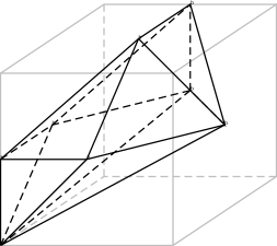
Figure 1. The polytope $\Delta_{f}^{\vee}$ for $X_{1-6}$

Example V.21 ($X_{1-4}$, $X_{1-5}$, $X_{1-7}$, and $X_{1-8}$).

Consider the Laurent polynomial $f$ from Table LABEL:table:_Fano_rank_1 for $X_{1-i}$, $i\in\{4,5,7,8\}$. Similar to the above example for $i=6$, one can check by hand that the polytope $\Delta_{f}^{*}$ satisfies the conditions of Theorem V.19. Thus, there is a degeneration of $X_{1-i}$ to the toric variety $T_{\Delta}$ corresponding to the Landau–Ginzburg model given by $f$.

Example V.22 ($X_{1-9}$).

Consider the Laurent polynomial $f$ from Table LABEL:table:_Fano_rank_1 for $X_{1-9}$. Here, $\nabla=\Delta_{f}^{*}$ has $12$ lattice points, so we cannot apply Theorem V.19, but similar techniques may be used to show the existence of the desired degeneration. Indeed, the dimension of the component $U$ corresponding to $X_{1-9}$ in the Hilbert scheme $\mathcal{H}_{X_{1-9}}$ of its anticanonical embedding is $153$, see [CI14, Proposition 4.1]. The variety $T_{\Delta}$, where $\Delta=N(f)$, corresponds to a point $[T_{\Delta}]$ in $\mathcal{H}_{X_{1-9}}$ since its Hilbert polynomial agrees with that of $X_{1-9}$. A standard deformation-theoretic calculation shows that $[T_{\Delta}]$ is a smooth point on a component of dimension 153. It remains to be shown that this component is in fact $U$.

Now, $\nabla=\Delta^{\vee}$ admits a regular unimodular triangulation such that the origin is contained in every full-dimensional simplex, one boundary vertex has valency $6$, and every other vertex has valency $4$ or $5$. The boundary of this triangulation is in fact the unique triangulation of the sphere with these properties. In any case, $T_{\Delta}$ degenerates to the Stanley–Reisner scheme $R$ corresponding to this triangulation, and $X_{1-9}$ does as well, see [CI14, Corollary 3.3]. Furthermore, a standard deformation-theoretic calculation shows that at the point $[R]$, $\mathcal{H}_{X_{1-9}}$ has only one $153$-dimensional component. Thus, $[T_{\Delta}]$ must lie on $U$, and $X_{1-9}$ must degenerate to $T_{\Delta}$.

Thus, independently from [DHKLP] and [IKKPS], we proved the following theorem (cf. Corollary V.12).

Theorem V.23.

Each Fano threefold of rank 1 has a toric weak Landau–Ginzburg model.

Proof.

According to [CCGK16], Laurent polynomials from Table LABEL:table:_Fano_rank_1 are weak Landau–Ginzburg models of the corresponding Fano varieties. According to Theorem V.9, they satisfy the Calabi–Yau condition. Thus the last thing needed to check is the toric condition. The varieties $X_{1-i}$, $i\in\{1,2,3,4,11,12,13,14\}$, are complete intersections in weighted projective spaces, so the toric condition for them follows from Theorem VII.35. The varieties $X_{1-10}$ and $X_{1-15}$ have small toric degenerations (i, e. degenerations to terminal Gorenstein toric varieties), so the toric condition for them follows from [Gal08]. The toric condition for $X_{1-i}$, $i\in\{5,6,7,8\}$, follows from Examples V.20 and V.21. The toric condition for $X_{1-9}$ follows from Example V.22. Finally, $X_{1-17}={\mathbb{P}}^{3}$ is toric. ∎

V.4. Modularity

In this section we present results from [DHKLP], see also [ILP13].

Mirror Symmetry predicts that fibers of Landau–Ginzburg model for a Fano variety are Calabi–Yau varieties. More precise, it is expected that these fibers are mirror dual to anticanonical sections of the Fano variety. In the threefold case this duality is nothing but Dolgachev–Nikulin duality of K3 surfaces.

Let $H$ be a hyperbolic lattice, ${\mathbb{Z}}\oplus{\mathbb{Z}}$ with intersection form

$$\left(\begin{array}[]{cc}0&1\\ 1&0\\ \end{array}\right).$$

The intersection lattice on the second cohomology on any K3 surface is

$$N=H\oplus H\oplus H\oplus E_{8}(-1)\oplus E_{8}(-1).$$

Consider a family $U_{K}$ of K3 surfaces whose lattice of algebraic cycles contains $K\subset N$ (and coincides with $K$ for general K3 surface). Consider a lattice $L^{\prime}=K^{\bot}$, the orthogonal to $K$ in $N$. Let $L^{\prime}=H\oplus L$.

Definition V.24 (see [Do01]).

The family of K3 surfaces $U_{L}$ is called the Dolgachev–Nikulin dual family to $U_{K}$.

Consider a principally polarized family of anticanonical sections of a Fano threefold $X$ of index $i$ and degree $(-K_{X})^{3}=i^{3}k$. It is nothing but $U_{\langle 2n\rangle}$, $2n=ik$, where $\langle r\rangle$ is a rank $1$ lattice generated by vector whose square is $r$. The lattice $U_{\langle 2n\rangle}$ is a sublattice of $H$. Using this embedding to one of the $H$-summands of $N$ we can see that Dolgachev–Nikulin dual lattice to $U_{\langle 2n\rangle}$ is the lattice

$$M_{n}=H\oplus E_{8}(-1)\oplus E_{8}(-1)+\langle-2n\rangle.$$

The surfaces with Picard lattices $M_{n}$ are Shioda–Inose. They are resolutions of quotients of specific K3 surfaces $S$ by Nikulin involution, the one keeping the transcendental lattice $T_{S}$; it changes two copies of $E_{8}(-1)$. Another description of Shioda–Inose surfaces is Kummer ones going back to products of elliptic curves with $n$-isogenic ones. $M_{n}$-polarized Shioda–Inose surfaces form an $1$-dimensional irreducible family.

It turnes out that fibers of toric Landau–Ginzburg models from Table LABEL:table:_Fano_rank_1 can be compactified to Shioda–Inose surfaces dual to anticanonical sections of Fano threefolds. In this section we prove the following.

Theorem V.25 ([DHKLP]).

Let $X$ be a Fano threefold of Picard rank $1$, index $i$ and let $(-K_{X})^{3}=i^{3}k$. Then a general fiber of toric weak Landau–Ginzburg model from Table LABEL:table:_Fano_rank_1 is a Shioda–Inose surface with Picard lattice $M_{ik/2}$.

We say that toric Landau–Ginzburg model for $X$ satisfies the Dolgachev–Nikulin condition if the assertion of Theorem V.25 holds for it. We call such toric Landau–Ginzburg model good.

Thus compactifications of the Landau–Ginzburg models are, modulo coverings and the standard action of action of $PSL(2,{\mathbb{C}})$ on the base, the unique families of corresponding Shioda–Inose surfaces. More precise, they are index-to-one coverings of the moduli spaces.

Corollary V.26 (cf. [DHNT17]).

A Calabi–Yau compactification of good weak Landau–Ginzburg model is unique up to flops.

Thus, if Homological Mirror Symmetry conjecture holds for Picard rank one Fano threefolds, then their Landau–Ginzburg models (in the Homological Mirror Symmetry sense) up to flops are compactifications of toric ones from Table LABEL:table:_Fano_rank_1. Moreover, all other good toric Landau–Ginzburg models are birational (over ${\mathbb{A}}^{1}$) to them.

To prove Theorem V.25 we study all $17$ one-by-one and compute Neron–Severi lattices of the compactified toric Landau–Ginzburg models.

Remark V.27.

In [Go07] Golyshev described Landau–Ginzburg models for Picard rank one Fano threefolds as universal families over $X_{0}(n)/\tau$, where $\tau$ is an Atkin–Lehner involution, with fibers that are Kummer surfaces associated with products of elliptic curves by an $n$-isogenic ones. Golyshev’s description of periods of these dual families as modular forms seems to be natural to expect from this point of view. The variations of Hodge structures of our families of Shioda–Inose surfaces are the same (over ${\mathbb{Q}}$) as the variations for the products of elliptic curves and the same over ${\mathbb{Z}}$ as for the Kummer surfaces; this follows from the description of Shioda–Inose surfaces given above.

Remark V.28.

Fibers of Landau–Ginzburg models are expected to be Dolgachev–Nikulin dual to anticanonical sections of Fano varieties of any Picard rank. As the Picard rank of the Fano increase, the mirror K3 fibers will no longer be Shioda–Inose. However they are still K3 surfaces of high Picard rank, so we can hope to find analogous modular-type properties (say, automorphic) in these cases as well. Say, fibers of Landau–Ginzburg models are Kummer surfaces given by products of elliptic curves for the Picard rank $2$ case and by abelian surfaces for the Picard rank $3$ case. These lattices are computed over ${\mathbb{Q}}$ in [CP18]; however the computations over ${\mathbb{Z}}$ need more deep methods.

V.4.1. Lattice facts

If $L$ is a lattice and $k$ a field, we will write $L_{k}$ for $L\otimes_{\mathbb{Z}}k$. We will use $\mathcal{N},\mathcal{M}$ to denote two dual rank-three lattices. Let $f_{1-i}$ denote the Laurent polynomial defining the Landau–Ginzburg model from Table LABEL:table:_Fano_rank_1 that correspond to $X_{1-i}$, let $\Delta_{f_{1-i}}^{*}\subset\mathcal{M}_{\mathbb{R}}$ be its Newton polytope, and let $\nabla_{f_{1-i}}\subset\mathcal{N}_{\mathbb{R}}$ be its polar.

Via $A_{n},D_{n},E_{n}$ we denote the root lattices of the corresponding Dynkin diagrams. Via $M$ we denote the rank 18 lattice $H\oplus E_{8}(-1)\oplus E_{8}(-1)$, and via $M_{n}$ the rank 19 lattice $M\oplus\langle-2n\rangle$.

We will use $(x:y:z:w)$ as homogeneous coordinates on ${\mathbb{P}}^{3}$. For distinct, non-empty subsets $I,J,K\subset\{1,2,3,4\}$, we will write $H_{I}$ for the hyperplane defined by setting the sum of coordinates in $I$ equal to zero. Thus, for example, $H_{\{1\}}$ is the coordinate hyperplane $x=0$, while $H_{\{2,4\}}$ is the hyperplane defined by $y+w=0$. We write $L_{I,J}=H_{I}\cap H_{J}$, and $p_{I,J,K}=H_{I}\cap H_{J}\cap H_{K}$.

In many cases, we will use Calabi–Yau compactifications that are different from those from Section V.2. That is, we use compactifications given by

$$({\mathbb{C}}^{*})^{3}\hookrightarrow{\mathbb{P}}[x:y:z:w],$$

cf. Section VI.3. This gives precise descriptions of fibers of compactifications as quartics in ${\mathbb{P}}^{3}$ with ordinary double points. In those cases, we will identify some curves on the minimal resolutions of these singular quartics (which will be K3 surfaces) and compute the intersection matrix of the identified curves, then checking that this matrix has rank 19. In the interest of not boring the reader to death, we will omit the details of these computations. In other cases, we will use elliptic fibrations as described below.

Because we will use them later, we recall a few (perhaps not terribly well-known) facts about lattices. Most are due to [Nik80]; a very readable reference is [Be02]. Let $L$ be a lattice, and $\langle\cdot,\cdot\rangle$ the bilinear pairing on $L$. Denote by $L^{*}$ the dual lattice $\mathrm{Hom}(L,{\mathbb{Z}})$. Since the pairing induces an isomorphism $L_{{\mathbb{Q}}}\simeq\mathrm{Hom}(L_{\mathbb{Q}},{\mathbb{Q}})$, we may think of $L^{*}\subset L_{\mathbb{Q}}$. The pairing $\langle\cdot,\cdot\rangle$ induces a quadratic form $q_{L}$ on the discriminant group $D(L)=L^{*}/L$ by $q_{L}(\phi)=\langle\phi,\phi\rangle$. A priori, $q_{L}$ takes values in ${\mathbb{Q}}/{\mathbb{Z}}$, but if $L$ is an even lattice, it will take values in ${\mathbb{Q}}/(2{\mathbb{Z}})$.

Fixing a basis $e_{1},\ldots e_{r}$ for $L$, we may form the Gram matrix $I_{L}$ whose $(i,j)$-th entry is $\langle e_{i},e_{j}\rangle$. We call $d(L)=\det(I_{L})$ the determinant of $L$.

Fact V.29.

Let $L$ be an even, indefinite lattice of rank $r$ and signature $(s,r-s)$, and let $d$ be the minimal number of generators of $L^{*}/L$. If $r>d+2$, then $q_{L}$ and $s$ uniquely determine $L$.

Fact V.30.

Let $L\subset M$ be even lattices of the same rank. Then $[M:L]^{2}=d(L)/d(M)$.

Fact V.31.

Let $L\subset M$ be even lattices of the same rank, and let $G=M/L\subset L^{*}/L=D$. Note since $L\subset M\subset M^{*}\subset L^{*}$, we have $G\subset M^{*}/L\subset D$ and $(M^{*}/L)/G\simeq M^{*}/M$. Now let $G^{\perp}=\{a\in D\>|\>q_{L}(a+H)=q_{L}(a)\}$. Since $M$ is even, $q_{L}|_{G}=0$, and hence $G\subset G^{\perp}$. Moreover, given $a\in D$, choose $\tilde{a}\in L^{*}$ such that $a=\tilde{a}+L$. Then $a\in G^{\perp}$ if and only if $\langle\tilde{a},M\rangle\subset{\mathbb{Z}}$, i.e. $G^{\perp}=M^{*}/L$. Thus we see that the quadratic form $q_{M}$ is nothing but $q_{L}|_{G^{\perp}}$ descended to $G^{\perp}/G$.

Conversely, given a subgroup $G\subset D$ such that $q_{L}(G)=0$, there exists a lattice $M$ containing $L$ such that $M/L=G$.

Fact V.32.

Let $L$ be a sublattice of a unimodular lattice $\Lambda$. Then $D(L)\simeq D(L^{\perp})$ and $q_{L}=-q_{L^{\perp}}$.

For convenience, we also include the discriminant groups and forms of some of the lattices that play a role in the present study. In Table 2 we present the discriminant form by giving its values on generators of the discriminant group. Note that this description is not unique. For example, if the discriminant group is ${\mathbb{Z}}/(8)$ and the form is listed as $1/8$, this means that a generator $g$ of the group has $q(g)=1/8$. Of course, $3g$ is also a generator, and it has $q(3g)=9/8$.

Lattice $L$	Group $D(L)$	Form $q_{L}$
$H$	$\{1\}$	$0$
$\langle-2n\rangle$	${\mathbb{Z}}/(2n)$	$-1/(2n)$
$A_{1}$	${\mathbb{Z}}/(2)$	$-1/2$
$A_{2}$	${\mathbb{Z}}/(3)$	$4/3$
$A_{3}$	${\mathbb{Z}}/(4)$	$5/4$
$A_{4}$	${\mathbb{Z}}/(5)$	$4/5$
$A_{5}$	${\mathbb{Z}}/(6)$
$A_{6}$	${\mathbb{Z}}/(7)$	$2/7$
$A_{7}$	${\mathbb{Z}}/(8)$	$1/8$
$A_{8}$	${\mathbb{Z}}/(9)$	$4/9$
$A_{9}$	${\mathbb{Z}}/(10)$	$-9/10$
$A_{10}$	${\mathbb{Z}}/(11)$	$4/11$
$A_{11}$	${\mathbb{Z}}/(12)$	$-11/12$
$D_{5}$	${\mathbb{Z}}/(4)$	$-5/4$
$D_{8}$	${\mathbb{Z}}/(2)\oplus{\mathbb{Z}}/(2)$	$0,1$
$D_{10}$	${\mathbb{Z}}/(2)\oplus{\mathbb{Z}}/(2)$	$1,1$
$E_{6}$	${\mathbb{Z}}/(3)$	$2/3$
$E_{7}$	${\mathbb{Z}}/(2)$	$1/2$
$E_{8}$	$\{1\}$	$0$

Table 2. Some Discriminant Groups and Forms

V.4.2. Elliptic fibrations on K3 surfaces

We briefly recall a few facts about elliptic fibrations with section on K3 surfaces.

Definition V.33.

An elliptic K3 surface with section is a triple $(X,\pi,\sigma)$, where $X$ is a K3 surface and $\pi:X\to{\mathbb{P}}^{1}$ and $\sigma:{\mathbb{P}}^{1}\to X$ are morphisms with the generic fiber of $\pi$ an elliptic curve and $\pi\circ\sigma=\mathrm{id}_{{\mathbb{P}}^{1}}$.

Any elliptic curve over the complex numbers can be realized as a smooth cubic curve in ${\mathbb{P}}^{2}$ in Weierstrass normal form

(V.34) $$y^{2}z=4x^{3}-g_{2}xz^{2}-g_{3}z^{3}.$$

Conversely, the equation (V.34) defines a smooth elliptic curve provided $\Delta=g_{2}^{3}-27g_{3}^{2}\neq 0$.

Similarly, an elliptic K3 surface with section can be embedded into the ${\mathbb{P}}^{2}$ bundle ${\mathbb{P}}(\mathcal{O}_{{\mathbb{P}}^{1}}\oplus\mathcal{O}_{{\mathbb{P}}^{1}}(4)\oplus\mathcal{O}_{{\mathbb{P}}^{1}}(6))$ as a subvariety defined by equation (V.34), where now $g_{2},g_{3}$ are global sections of $\mathcal{O}_{{\mathbb{P}}^{1}}(8)$, $\mathcal{O}_{{\mathbb{P}}^{1}}(12)$ respectively (i.e. they are homogeneous polynomials of degrees 8 and 12). The singular fibers of $\pi$ are the roots of the degree 24 homogeneous polynomial $\Delta=g_{2}^{3}-27g_{3}^{2}\in H^{0}(\mathcal{O}_{{\mathbb{P}}^{1}}(24))$. Tate’s algorithm can be used to determine the type of singular fiber over a root $p$ of $\Delta$ from the orders of vanishing of $g_{2}$, $g_{3}$, and $\Delta$ at $p$.

Proposition V.35.

[CD07, Lemma 3.9] A general fiber of $\pi$ and the image of $\sigma$ span a copy of $H$ in $\mathrm{Pic}(X)$. Further, the components of the singular fibers of $\pi$ that do not intersect $\sigma$ span a sublattice $S$ of $\mathrm{Pic}(X)$ orthogonal to this $H$, and $\mathrm{Pic}(X)/(H\oplus S)$ is isomorphic to the Mordell–Weil group $MW(X,\pi)$ of sections of $\pi$.

Proposition V.36.

[Mi89, Corollary VII.3.1] The torsion subgroup of $MW(X,\pi)$ embeds in $D(S)$.

When K3 surfaces are realized as hypersurfaces in toric varieties, one can construct elliptic fibrations combinatorially. As before, let $\Delta\subset\mathcal{N}_{\mathbb{Q}}$ be a reflexive polytope, and suppose $P\subset\mathcal{N}$ is a plane such that $\Delta\cap P$ is a reflexive polygon $\nabla$. Let $m\in\mathcal{M}=\mathcal{N}^{\vee}$ be a normal vector to $P$. Then $P$ induces a torus-invariant map ${\mathbb{P}}(\Delta^{*})\to{\mathbb{P}}^{1}$ with generic fiber ${\mathbb{P}}_{\nabla}$, given in homogeneous coordinates by

$$\pi_{m}:(z_{1},\ldots z_{r})\mapsto\left[\prod_{\langle v_{i},m\rangle>0}z_{i}^{\langle v_{i},m\rangle},\prod_{\langle v_{i},m\rangle<0}z_{i}^{-\langle v_{i},m\rangle}\right].$$

Restricting $\pi_{m}$ to an anticanonical K3 surface, we get an elliptic fibration. If $\nabla$ has an edge without interior points, this fibration will have a section as well. See [KS02] for more details.

V.4.3. Picard lattices of fibers of the Landau–Ginzburg models

1. Recall that a Landau–Ginzburg model of Givental type for $X_{1-1}$ is

   $$\left\{\begin{array}[]{ll}y_{0}y_{1}y_{2}y_{3}y_{4}^{3}=1\\ y_{1}+y_{2}+y_{3}+y_{4}=1\end{array}\right.$$

   with superpotential

   $$w=y_{0}.$$

   Consider the change of variables

   $$y_{1}=\frac{x}{x+y+z+t},\ \ y_{2}=\frac{y}{x+y+z+t},\ \ y_{3}=\frac{z}{x+y+z+t},\ \ y_{4}=\frac{t}{x+y+z+t},$$

   where $x,y,z,t$ are projective coordinates. We get the Landau–Ginzburg model

   $$y_{0}xyzt^{3}=(x+y+z+t)^{6},\ \ \ \ w=y_{0}.$$

   Thus in the local chart, say, $t\neq 0$ we get the toric Landau–Ginzburg model from Table LABEL:table:_Fano_rank_1

   $$f_{1-1}=\frac{(x+y+z+1)^{6}}{xyz}.$$

   A general element of the pencil that correspond to $f_{1-1}$ is birational to the general element of the initial Landau–Ginzburg model. Inverse the superpotential: $u=1/w$. We get the pencil given by

   $$y_{1}y_{2}y_{3}y_{4}^{3}=u,\ \ \ \ y_{1}+y_{2}+y_{3}+y_{4}=1.$$

   This is the Landau–Ginzburg model for weighted projective space ${\mathbb{P}}(1:1:1:3)$, see [CG11, (2)]. (In particular, by [CG11, Theorem 1.15] its general element is birational to a K3 surface.) However make another change of variables in the Givental’s Landau–Ginzburg model putting $x=y_{1}$, $y=y_{2}$, $z=y_{4}$. We get the family given by

   $$\widetilde{f}_{1-1}=x+y+z+\frac{w}{xyz^{3}}-1=0$$

   Let $\widetilde{\Delta}_{f_{1-1}}$ be a Newton polytope of the polynomial $\widetilde{f}_{1-1}$ and let $\widetilde{\nabla}_{f_{1-1}}=\widetilde{\Delta}_{f_{1-1}}^{\vee}$. Then fibers of the pencil $\{\widetilde{f}_{1-1}=0\}$ can be compactified inside $T_{\widetilde{\nabla}_{f_{1-1}}}$, cf. Section V.2. The normal vector $(1,2,3)$ induces an elliptic fibration with a section. The Weierstrass form of the fibers of the elliptic fibration is

   $$-\frac{t^{4}u}{48}+\frac{1}{864}t^{5}\left(864t^{2}+1728t\lambda-t+864\lambda^{2}\right)+u^{3}+v^{2}=0.$$

   Hence by Tate’s algorithm there are singular fibers of type $II^{*}$ at $t=0,\infty$ and $I_{2}$ at $t=-\lambda$. Therefore, the K3 surfaces in question are polarized by $H\oplus E_{8}(-1)\oplus E_{8}(-1)\oplus A_{1}(-1)=M_{1}.$

   There is also another fibration induced by the normal $(1,0,1)$ which gives a polarization by

   $$H\oplus E_{7}(-1)\oplus D_{10}(-1).$$

2. Compactify this family to the family of quartics $(x+y+z+w)^{4}-\lambda xyzw=0$ in ${\mathbb{P}}^{3}$. Intersecting the quartic with the pencil of planes containing one of lines lying on it gives a pencil of divisors with the line as base locus. Subtracting the line gives a pencil of cubics. Blowing up the base points of this pencil gives an elliptic fibration with section, which gives a polarization of the K3 surfaces by $H\oplus E_{6}(-1)\oplus A_{11}(-1)$. This fibration has a 3-torsion section, and it can have no other torsion sections by Proposition V.36. Thus by Fact V.30, the generic fiber $X$ of $f_{1-2}$ has $d(NS(X))=4$. As we shall see, fibers of the Landau–Ginzburg model $X_{1-17}={\mathbb{P}}^{3}$ have fibrations of this type as well, and comparing parameters of the two Weierstrass equations, we see that fibers of compactified toric Landau–Ginzburg models for $X_{1-1}$ and $X_{1-17}$ are the same. Because generic fibers of compactifications for $f_{1-17}$ are $M_{2}$-polarized (as we will see soon), $NS(X)\simeq M_{2}$.

3. Compactify the fibers of $f_{1-3}$ as a family of anticanonical divisors in ${\mathbb{P}}^{1}\times{\mathbb{P}}^{2}$ via $(x,y,z)\mapsto((x:1)\times(y:z:1))$. Explicitly, $f_{1-3}^{-1}(\lambda)$ compactifies to the K3 surface

   $$Y_{\lambda}=\{((x:x_{0}),(y:z:w))\in{\mathbb{P}}^{1}\times{\mathbb{P}}^{2}\>|\>(x+x_{0})^{2}(y+z+w)^{3}-\lambda xx_{0}yzw=0\}.$$

   The projection ${\mathbb{P}}^{1}\times{\mathbb{P}}^{2}\to{\mathbb{P}}^{1}$ induces an elliptic fibration on $Y_{\lambda}$ for generic $\lambda$. The map $(x:x_{0})\mapsto((x:x_{0}),(1:-1:0))$ gives a section of this elliptic fibration. Putting the fiber over $(1:a)$ into Weierstrass form

   $$\frac{a^{3}\lambda^{3}(24(1+a)^{2}-a\lambda)}{48}X-\frac{a^{4}\lambda^{4}(36(1+a)^{2}(6(1+a)^{2}-as)+a^{2}s^{2})}{864}+X^{3}+Y^{2}=0$$

   and using Tate’s algorithm, we see singular fibers of Kodaira type $IV^{*}$ at $a=0,\infty$; $I_{6}$ at $a=-1$; and $I_{1}$ where $27(a+1)^{2}-\lambda a=0$. Hence the rank 19 lattice $H\oplus E_{6}(-1)\oplus E_{6}(-1)\oplus A_{5}(-1)$ embeds in the Picard lattice of $Y_{\lambda}$.

   As we will see later, the fibers of $f_{1-16}$ also have fibrations of this type and are $M_{3}$-polarized. Matching the Weierstrass equations, we conclude that fibers for $f_{1-3}$ are isomorphic to fibers for $f_{1-16}$, and hence fibers for $f_{1-3}$ must also be $M_{3}$-polarized.

4. Similar to the case above, we compactify the family as anticanonical K3 surfaces in ${\mathbb{P}}^{1}\times{\mathbb{P}}^{1}\times{\mathbb{P}}^{1}$. Projection onto one of the ${\mathbb{P}}^{1}$ factors gives the generic K3 fiber an elliptic fibration with section. Putting this into Weierstrass form and running Tate’s algorithm give us an embedding of the rank 19 lattice $H\oplus A_{7}(-1)\oplus D_{5}(-1)\oplus D_{5}(-1)$ into the Picard lattice of the generic fiber. Moreover, the Mordell–Weil group is isomorphic to ${\mathbb{Z}}/(4)$. Applying the lattice facts above, with $L=H\oplus A_{7}\oplus D_{5}\oplus D_{5}$, $M=NS(X)$, $G=MW(X)\simeq{\mathbb{Z}}/(4)$, and $D=L^{*}/L\simeq{\mathbb{Z}}/(8)\oplus{\mathbb{Z}}/(4)\oplus{\mathbb{Z}}/(4)$, we have that $d(M)=8$. Examining the possibilities for $G\subset D$, we conclude $M^{*}/M\simeq{\mathbb{Z}}/(8)$, and that $q_{M}$ of a generator is $7/8$.

   Now we claim that $M\simeq M_{4}$. Let $e$ be a generator of the $\langle-8\rangle$ direct summand of $M_{4}$. Since $H$ and $E_{8}$ are unimodular, the group $M_{4}^{*}/M_{4}\simeq{\mathbb{Z}}/(8)$ is generated by $\epsilon=\frac{1}{8}e$, and $q_{M_{4}}(\epsilon)=-1/8$. Note that the element $3\epsilon$ also generates $M_{4}^{*}/M_{4}$, and $q_{M_{4}}(3\epsilon)=-9/8\equiv 7/8\>(mod\ 2{\mathbb{Z}})$. Thus we see that $M$ and $M_{4}$ have the same discriminant form, and their ranks are sufficiently large relative to the number of generators of the discriminant groups. Hence by Fact V.29 one gets that $M$ and $M_{4}$ must be isomorphic.

5. Compactify fibers to singular quartics. There are singularities at $p_{\{i\},\{j\},\{4\}}$ for $1\leqslant i\neq j\leqslant 3$ of type $\mathbb{D}_{4}$ and at $p_{\{i\}\{j\},\{k,4\}}$ where $\{i,j,k\}=\{1,2,3\}$ of type $\mathbb{A}_{1}$. Thus the exceptional curves generate a sublattice of rank 15. The quartics also contain lines $L_{\{i\},\{j,4\}}$ and conics $C_{\{i,j,4\}}$ for $1\leqslant i\neq j\leqslant 3$, subject to relations from

   $$H_{\{1\}} = 2L_{\{1\},\{2,4\}}+2L_{\{1\},\{3,4\}},$$

   $$H_{\{2\}} = 2L_{\{2\},\{1,4\}}+2L_{\{2\},\{3,4\}},$$

   $$H_{\{3\}} = 2L_{\{3\},\{1,4\}}+2L_{\{3\},\{2,4\}},$$

   $$H_{124} = L_{\{1\}\{2,4\}}+L_{\{2\},\{1,4\}}+C_{\{1,2,4\}},$$

   $$H_{\{1,3,4\}} = L_{\{1\},\{3,4\}}+L_{\{3\},\{1,4\}}+C_{\{1,3,4\}},$$

   $$H_{\{2,3,4\}} = L_{\{2\},\{3,4\}}+L_{\{3\},\{2,4\}}+C_{\{2,3,4\}},$$

   which leave a lattice of rank 19.

   Explicitly computing the intersection matrix for the identified curves (one needs to blow up singular curves for this and figure out how strict images of the curves intersect exceptional curves, see Proposition VI.49) shows that they generate a lattice with determinant 10, discriminant group ${\mathbb{Z}}/(10)$ with a generator $\alpha$ having $q(\alpha)=11/10$. Choosing instead the generator $\beta=3\alpha$, we have

   $$q(\beta)=99/10\equiv-1/10\ (mod\ 2{\mathbb{Z}}).$$

   Hence this lattice is isomorphic to $M_{5}$.

   We have just show that for $X$ a general K3 in this pencil, $NS(X)$ contains $M_{5}$. To see that $NS(X)$ actually equals $M_{5}$, we note that since $M$ is unimodular and contained in $NS(X)$, it must be a direct summand. Because $NS(X)$ is an even lattice of signature (1,18), the orthogonal complement of $M\subset NS(X)$ must be even, negative definite, and rank 1 and hence be equal to $\langle-2n\rangle$ for some $n$. From Fact V.30, $10/(\det NS(X))=5/n$ must be a square, and hence $n=5$.

   Alternately, the intersection of one of the singular quartics with a plane containing $L_{\{1\},\{2,4\}}$ consists of $L_{\{1\},\{2,4\}}$ and a (generically) smooth cubic. The pencil of these cubics, with base points blown up, give an elliptic fibration on the minimal resolution of the quartic. This fibration has singular fibers of types $I_{2}^{*}$, $I_{1}^{*}$, $I_{6}$, and 3 ones of type $I_{1}$. It also has a section of infinite order and a 2-torsion section. Hence the Picard lattice of the generic member of this family is a rank 19 lattice containing

   $$H\oplus D_{6}(-1)\oplus D_{5}(-1)\oplus A_{5}(-1)$$

   with quotient ${\mathbb{Z}}\oplus{\mathbb{Z}}/(2)$.

6. Again, we can compactify the fibers for $f_{1-6}$ to singular quartics in the standard way. There are $\mathbb{A}_{1}$ singularities at $(1:-1:0:0)$, $(1:0:-1:0)$, and $(0:1:-1:0)$; $\mathbb{A}_{2}$ singularities at $(1:0:0:0)$ and $(0:0:1:-1)$; and $\mathbb{A}_{3}$ singularities at $(0:1:0:0)$ and $(1:0:0:-1)$. These quartics also contain twelve lines:

   $$L_{\{1\},\{2,3\}},L_{\{1\},\{3,4\}},L_{\{1\},\{2,3,4\}},L_{\{2\},\{3\}},L_{\{2\},\{3,4\}},L_{\{2\},\{1,3,4\}},$$

   $$L_{\{3\},\{4\}},L_{\{3\},\{1,4\}},L_{\{3\},\{1,2,4\}},L_{\{4\},\{1,3\}},L_{\{4\},\{2,3\}},L_{\{4\},\{1,2,3\}}$$

   subject to relations coming from setting equal the hyperplane sections $H_{\{1\}}$, $H_{\{2\}}$, $H_{\{3\}}$, $H_{\{4\}}$, $H_{\{1,3,4\}}$, $H_{\{1,2,3,4\}}$, $H_{\{3,4\}}$, and $H_{\{2,3\}}$. These relations show that only six of these twelve lines are linearly independent. Hence the exceptional locus and strict transforms of lines generate a sublattice of the Picard lattice of the minimal resolutions of K3 surfaces of rank 13+6 =19.

   By explicitly computing the intersection matrix for the 25 rational curves identified, we conclude that the lattice they generate has determinant $\pm 12$, discriminant group ${\mathbb{Z}}/(12)$, and discriminant form $23/12\equiv-1/12\ ({mod}\ 2{\mathbb{Z}})$. Hence this lattice is isomorphic to $M_{6}$. Similar to the argument in the case for $X_{1-5}$, Fact V.30 shows that the Picard lattice must be equal to $M_{6}$.

7. Again, we compactify fibers to singular quartics. The quartics are defined by

   $$(x+y+z+w)(yz(x+y+z+w)+(y+z+w)(z+w)^{2})-\lambda xyzw=0.$$

   The singularities are: type $\mathbb{A}_{1}$ at $(0:1:0:-1)$, type $\mathbb{A}_{2}$ at $(1:0:0:0)$, $(0:1:-1:0)$, and $(\lambda:0:-1:1)$, type $\mathbb{A}_{3}$ at $(0:0:1:-1)$, and type $\mathbb{A}_{4}$ at $(1:-1:0:0)$. The quartics contain eight lines

   $$L_{\{i\},\{1,2,3,4\}}\ (1\leqslant i\leqslant 4),\ L_{\{2\},\{3,4\}},\ L_{\{3\},\{2,4\}},$$

   $$L_{\{3\},\{4\}},L_{\{234\},*}=\{y+z+w=x-\lambda w=0\}$$

   and two conics

   $$C_{1}=\{x=yz+(z+w)^{2}=0\},\ C_{4}=\{w=xy+(y+z)^{2}=0\}$$

   subject to relations coming from setting equal the hyperplane sections $H_{\{1\}}$, $H_{\{2\}}$, $H_{\{3\}}$, $H_{\{4\}}$, $H_{\{2,3,4\}}$, and $H_{\{1,2,3,4\}}$. These relations show that these 10 rational curves on the quartic generate a sublattice of rank 5 in the Picard lattice. Hence the exceptional locus and the strict transforms of these 10 curves generate a rank 19 sublattice of the Picard lattice of the minimal resolution.

   Explicitly computing the intersection matrix for the curves identified shows they generate a lattice isomorphic to $M_{7}$. Hence as in the cases above, the Picard lattice of the general fiber is $M_{7}$.

8. Compactifying to singular quartics gives singularities of type $\mathbb{A}_{1}$ at

   $$(-1:0:0:1),(0:-1:0:1),(0:0:-1:1),$$

   $$(1:-1:0:0),(1:0:-1:0),(0:1:-1:0),$$

   and of type $\mathbb{A}_{2}$ at

   $$(1:0:0:0),(0:1:0:0),(0:0:1:0).$$

   There are also 13 lines

   $$L_{\{i\},\{1,2,3,4\}},L_{\{j\},\{4\}},L_{\{j\},\{k,4\}}\>\mathrm{for}\>1\leqslant i\leqslant 4,\>1\leqslant j\neq k\leqslant 3,$$

   subject to relations from setting equal the hyperplane sections by $H_{\{i\}}$, $H_{\{j,4\}}$, and $H_{\{1,2,3,4\}}$ for $1\leqslant i\leqslant 4$, $1\leqslant j\leqslant 3$. These relations show that the lattice generated by the 13 lines has rank 7. Hence the strict transforms of the lines and the exceptional locus generate a lattice of rank 19.

   By explicitly computing the intersection matrix for the 25 rational curves identified, we conclude that the lattice they generate has determinant $\pm 16$, and discriminant group ${\mathbb{Z}}/(16)$ with a generator $\alpha$ such that $q(\alpha)=23/16$. Taking $\beta=5\alpha$ as generator, we have $q(\beta)=575/16\equiv-1/16\ (\mathrm{mod}\ 2{\mathbb{Z}})$. Hence this lattice is isomorphic to $M_{8}$. In this case, Fact V.30 shows that the Picard lattice of the generic K3 in the pencil is either $M_{8}$ or $M_{2}$. We now use the results of [Go07], which implies that this pencil has the same variation of Hodge structure as the $M_{8}$ pencil, and hence a different variation from the $M_{2}$ variation. Thus we conclude that this pencil must be $M_{8}$-polarized.

9. Compactify fibers to quadrics in ${\mathbb{P}}^{3}$ in the standard way. These quartics have an elliptic fibration with a section coming from intersections with planes containing $L_{\{4\},\{1,2,3\}}$ that gives a polarization of the Picard lattice of the minimal resolution by the rank 19 lattice

   $$H\oplus A_{8}(-1)\oplus A_{2}(-1)\oplus A_{1}(-1)\oplus E_{6}(-1).$$

   By Proposition V.36 there can be no sections of this fibration other than the zero section, and so the Picard lattice must be equal to

   $$H\oplus A_{8}(-1)\oplus A_{2}(-1)\oplus A_{1}(-1)\oplus E_{6}(-1)=M_{9}.$$

10. The quartic compactification contains lines

    $$L_{\{1\},\{3\}},L_{\{1\},\{4\}},L_{\{1\},\{2,4\}},L_{\{1\},\{3,4\}},L_{\{2\},\{3\}},L_{\{2\},\{4\}},L_{\{2\},\{1,4\}},L_{\{2\},\{3,4\}},L_{\{3\},\{1,4\}},$$

    $$L_{\{3\},\{2,4\}},L_{\{1,3\},\{4\}}L_{\{2,3\},\{4\}},L_{\{1,4\},*}=\{x+w=(s-2)x+y=0\},$$

    $$L_{\{2,4\},*}=\{y+w=(s-2)y+x=0\}$$

    and conics

    $$C_{\{3,4\}}=\{z+w=xy+(\lambda-2)z^{2}=0\},$$

    $$C_{\{1,2,4\}}=\{x+y+w=xy+(\lambda-3)(x+y)z+z^{2}=0\},$$

    $$C=\{z=(\lambda+1)w,(\lambda+1)w^{2}+xy=0\},$$

    $$C^{\prime}=\{z=(\lambda+1)w,2w(w+x+y)+\lambda w(x+y)+xy=0\}$$

    subject to relations coming from $H_{\{i\}}$, and singularities of type $\mathbb{A}_{3}$ at $(1:0:0:0)$ and $(0:1:0:0)$, type $\mathbb{A}_{2}$ at $(0:0:1:0)$, and type $\mathbb{A}_{1}$ at $(-1:0:0:1)$ and $(0:-1:0:1)$. The lines are subject to relations from setting equal $H_{\{1\}}$, $H_{\{2\}}$, $H_{\{3\}}$, $H_{\{4\}}$, $H_{\{1,3\}}$, $H_{\{2,3\}}$, $H_{\{1,4\}}$, $H_{\{2,4\}}$, and $H_{\{3,4\}}$.

    Computing the intersection matrix shows that the Picard lattice is $M_{10}$.

11. By Proposition V.11, the fibers we are interested in are birational to quartics

    $$\{x^{4}-(\lambda y-z)(xw-xy-w^{2})z=0\}.$$

    We may consider the elliptic fibration on the fibers for the family of quartics induced from intersections with planes containing $L_{\{1\},\{3\}}$. Putting this fibration into Weierstrass form and applying Tate’s algorithm gives a polarization by $H\oplus E_{7}(-1)\oplus D_{10}(-1)$. Comparing the Weierstrass form of this fibration to the Weierstrass form for the similar fibration for $f_{1-1}$, we conclude that the Picard lattice must be $M_{1}$.

12. Compactify the fibers of the pencil for $f_{1-12}$ to quartics in ${\mathbb{P}}^{3}$. Intersecting the quartics with the pencil of planes containing $L_{\{1\},\{2,4\}}$, subtracting this line, and blowing up base points gives an elliptic fibration with section on the K3 surfaces. The induced polarization is by the rank 19 lattice $H\oplus E_{6}(-1)\oplus A_{11}(-1)$. Comparing with the similar fibration for $X_{1-17}$, the generic lattice must be $M_{2}$.

13. Compactify the fibers of the pencil for $f_{1-13}$ to quartics in ${\mathbb{P}}^{3}$. Intersecting the quartics with planes containing the line $L_{\{1\},\{4\}}$ gives an elliptic fibration that results in a polarization by $H\oplus E_{6}(-1)\oplus E_{6}(-1)\oplus A_{5}(-1).$ The Mordell–Weil group of this fibration is ${\mathbb{Z}}/(3)$. Hence, applying lattice facts, $d(NS(X))=\pm 6$. In fact, by matching parameters with the similar fibrations for $X_{1-3}$ and $X_{1-16}$, we conclude that $NS(X)\simeq M_{3}$.

14. We can compactify the pencil in the toric variety $T_{\nabla_{f_{1-14}}}$ and consider the elliptic fibration with section induced by $(0,0,1)$. This yields a fibration with fibers of type $I_{8}$ at $\infty$ and $I_{1}^{*}$ at $t=\frac{1}{2}\left(\lambda\pm\sqrt{\lambda^{2}+16}\right)$. Hence the fibers carry a polarization by $H\oplus A_{7}(-1)\oplus D_{5}(-1)\oplus D_{5}(-1)$. Moreover, the Mordell–Weil group is isomorphic to ${\mathbb{Z}}/(4)$. So, as for $X_{1-4}$, these K3 surfaces are $M_{4}$-polarized.

15. Compactify the fibers for $f_{1-15}$ in $T_{\nabla_{f_{1-15}}}$. The vector $m=(1,1,0)$ induces an elliptic fibration on the generic compactified fiber $Y_{\lambda}$. The Weierstrass form of this fibration is

    $$-\frac{1}{48}t^{2}P(s,t)u+\frac{1}{864}t^{3}\left(s^{2}(-t)+4t^{2}+12t+8\right)\left(P(s,t)+24(1+t)^{2}\right)+u^{3}+v^{2}=0,$$

    where $P(s,t)=s^{4}t^{2}-8s^{2}t^{3}-24s^{2}t^{2}-16s^{2}t+16t^{4}+24t^{3}-8t^{2}-24t-8$. This fibration has a section of infinite order given by

    $$t\mapsto\left(-\frac{1}{12}t\left(s^{2}t+8t^{2}+12t+4\right),-\frac{1}{2}st^{2}(t+1)^{2}\right)=(u,v)$$

    and a 2-torsion section given by

    $$t\mapsto\left(\frac{1}{12}\left(-s^{2}t+4t^{2}+12t+8\right),0\right)=(u,v).$$

    Hence by Proposition V.35, the lattice $NS(X)$ is a rank 19 lattice containing $H\oplus D_{6}(-1)\oplus D_{5}(-1)\oplus A_{5}(-1)$ with the quotient ${\mathbb{Z}}\oplus{\mathbb{Z}}/(2)$. Matching this elliptic fibration with the one for $X_{1-5}$, we conclude that fibers for $f_{1-15}$ are isomorphic to fibers of $f_{1-5}$, and hence these K3 surfaces are $M_{5}$-polarized.

16. The vector $m=(1,2,1)$ defines an elliptic fibration with section on the generic fiber $Y_{\lambda}$ of the Landau–Ginzburg model. The Weierstrass form of this fibration is

    $$-\frac{1}{48}st^{3}u\left(s^{3}t+48t+48\right)+\frac{1}{864}t^{5}\left(s^{6}(-t)-\right.\\ \left.-72s^{3}t-72s^{3}+864t^{2}+1728t+864\right)+u^{3}+v^{2}=0,$$

    and there are singular fibers of types $III^{*}$ at $t=0$, $II^{*}$ at $t=\infty$, and $I_{3}$ at $t=-1$. Hence the K3 fiber is polarized by the rank 19 lattice $N\oplus A_{2}(-1)$. By Proposition V.36, there can be no torsion sections (the discriminant groups of the two singular fibers have coprime orders), so $NS(Y_{\lambda})=K\oplus A_{2}(-1)$, where $K=H\oplus E_{8}(-1)\oplus E_{7}(-1)$.

    Now note that $D(K\oplus A_{2}(-1))={\mathbb{Z}}/(2)\oplus{\mathbb{Z}}/(3)\simeq{\mathbb{Z}}/(6)$. If we write the isomorphism ${\mathbb{Z}}/(6)\to{\mathbb{Z}}/(2)\oplus{\mathbb{Z}}/(3)$ as $1\mapsto(1,1)$, then we can write the form $q_{N\oplus A_{2}}:{\mathbb{Z}}/(6)\to{\mathbb{Q}}/(2{\mathbb{Z}})$ by specifying

    $$q_{N\oplus A_{2}(-1)}(1)=1/2+4/3=11/6\equiv-1/6\ (mod\ 2{\mathbb{Z}}).$$

    Thus $q_{N\oplus A_{2}}\simeq q_{\langle-6\rangle}\simeq q_{M_{3}}$. Hence by Fact V.29, $NS(X)\simeq M_{3}$.

    Because it is useful for cases $X_{1-3}$ and $X_{1-13}$, we note that $m=(1,0,0)$ gives a fibration with lattice $H\oplus E_{6}(-1)\oplus E_{6}(-1)\oplus A_{5}(-1)$ plus additional sections.

17. Anticanonical K3’s in ${\mathbb{P}}^{3}$ have generic Picard lattice $\langle 4\rangle$ generated by the hyperplane section. We claim that the mirror family has rank 19 Picard lattice $M_{2}$. We can see this explicitly from the toric fibration on $T_{\nabla_{f_{1-17}}}$ defined by the normal vector $m=(1,-1,-2)$. Restricting this fibration to the generic fiber of the Landau–Ginzburg model gives the fiber the structure of an elliptic surface with Weierstrass equation

    $$-\frac{1}{48}\left(s^{4}+144\right)t^{4}u+\frac{1}{864}t^{5}\left(s^{6}(-t)+648s^{2}t+864t^{2}+864\right)+u^{3}+v^{2}=0.$$

    Applying Tate’s algorithm we see singular fibers of Kodaira type $II^{*}$ at $t=0,\infty$, and hence the K3 surfaces are $M$-polarized. Moreover,

    $$(u,v)=\left(-\frac{4s^{4}+120s^{2}+108}{12s^{2}},\frac{3\left(4s^{4}+30s^{2}+18\right)}{2s^{3}}\right)$$

    gives a section of infinite order in $MW(\pi_{m})$, enhancing the polarization to rank 19. Since these are $M$-polarized rank 19 K3 surfaces, they must be $M_{n}$ polarized for some $n$, and as in the case for $X_{1-8}$, we now appeal to [Go07] to conclude that the Picard lattice must be $M_{2}$.

Remark V.37 (cf. Remark V.27).

In [Go07] it is shown that the Landau–Ginzburg models for the cases under consideration have the same variation of Hodge structures (up to pullbacks) as modular variations associated to products of elliptic curves with isogeny. Explicitly, for $X$ one of the Fano threefolds under consideration, let $(N,d)=\left(\frac{\deg(X)}{2\cdot\mathrm{ind}(X)^{2}},\mathrm{ind}(X)\right)$. Let $X_{0}(N)+N$ denote the modular curve $\overline{(\Gamma_{0}(N)+N)\backslash\mathbb{H}}$, and let $t_{N}$ be a hauptmodul for $X_{0}(N)+N$ such that $t_{N}=0$ at the image of the cusp $i\infty$. The Picard–Fuchs equation for the Landau–Ginzburg model of $X$ is now the pullback of the symmetric square of the uniformizing differential equation for $X_{0}(N)+N$ by $\lambda=t_{N}^{d}$.

We can check that the pullback part of Golyshev’s theorem follows in a straightforward way from the geometry of the fibers of the Landau–Ginzburg model.

• Cases $X_{1-1}$ and $X_{1-11}$: Both have polarizations by $H\oplus E_{7}(-1)\oplus D_{10}(-1)$. Clearly, since the moduli space of $H\oplus E_{7}(-1)\oplus D_{10}(-1)$ polarized K3 surfaces is 1-dimensional, we see a posteriori that the Landau–Ginzburg models $f_{1-1}$ and ${f}_{1-11}$ have isomorphic K3-compactified fibers.

• Cases $X_{1-2}$ $X_{1-12}$, and $X_{1-17}$: Similarly, since the moduli space of K3 surfaces polarized by $H\oplus E_{6}(-1)\oplus A_{11}(-1)$ is 1-dimensional, we see a posteriori that the Landau–Ginzburg models $f_{1-2}$, $f_{1-12}$, and $f_{1-17}$ have isomorphic fibers. Writing the Weierstrass forms for the elliptic fibrations that give this polarization in each case, we can match the fibrations fiberwise to check that indeed fibers for $X_{1-12}$ are given from fibers for $X_{1-2}$ by pullback $\lambda\mapsto\lambda^{2}$ , and similarly the compactification for $X_{1-17}$ is a pullback $\lambda\mapsto\lambda^{4}$ of the compactification for $X_{1-17}$.

• $X_{1-3}$, $X_{1-13}$, and $X_{1-16}$: Similar to the previous cases, using the polarizations by $H\oplus E_{6}(-1)\oplus E_{6}(-1)\oplus A_{5}(-1)$.

• Cases $X_{1-4}$ and $X_{1-14}$: Similar to the previous cases, using the polarizations by $H\oplus A_{7}(-1)\oplus D_{5}(-1)\oplus D_{5}(-1)$.

• Cases $X_{1-5}$ and $X_{1-15}$: In this case, the pullback was used to derive the polynomial $f_{1-15}$.

Part VI Katzarkov–Kontsevich–Pantev conjectures

This part is based on papers [KKP17], [LP18], and [CP18]. We study here Katzarkov–Kontsevich–Pantev conjectures about Hodge numbers of Landau–Ginzburg models and prove them in the cases of dimension 2 and 3.

VI.1. Formulation

Let us recall some numerical conjectures from [KKP17] which are supposed to follow from the conjectural Homological Mirror Symmetry between Fano manifolds and Landau–Ginzburg models.

Definition VI.1.

A Landau–Ginzburg model is a pair $(Y,w)$, where

1. $Y$ is a smooth complex quasi-projective variety with trivial canonical bundle $K_{Y}$;

2. $w\colon Y\to{\mathbb{A}}^{1}$ is a morphism with a compact critical locus $crit(w)\subset Y$.

Remark VI.2.

Note that there are no conditions on singularities of fibers.

Following [KKP17] we assume that there exists a tame compactification of the Landau–Ginzburg model as defined below (cf. Definition III.6).

Definition VI.3.

A tame compactified Landau–Ginzburg model is the data $((Z,f),D_{Z})$, where

1. $Z$ is a smooth projective variety and $f\colon Z\to{\mathbb{P}}^{1}$ is a flat morphism.

2. $D_{Z}=(\cup_{i}D^{h}_{i})\cup(\cup_{j}D_{j}^{v})$ is a reduced normal crossings divisor such that

   • $D^{v}=\cup_{j}D^{v}_{j}$ is a scheme-theoretical pole divisor of $f$, i.e. $f^{-1}(\infty)=D^{v}$. In particular $ord_{D^{v}_{j}}(f)=-1$ for all $j$;

   • each component $D_{i}^{h}$ of $D^{h}=\cup_{i}D^{h}_{i}$ is smooth and horizontal for $f$, i.e. $f|_{D^{h}_{i}}$ is a flat morphism;

   • The critical locus $crit(f)\subset Z$ does not intersect $D^{h}$.

3. $D_{Z}$ is an anticanonical divisor on $Z$.

   One says that $((Z,f),D_{Z})$ is a compactification of the Landau–Ginzburg model $(Y,w)$ if in addition the following holds:

4. $Y=Z\setminus D_{Z}$, $f|_{Y}=w$.

Remark VI.4.

In [KKP17] the authors require in above definitions an additional choice of compatible holomorphic volume forms on $Z$ and $Y$. Since these forms will play no role in this paper we omitted them.

Assume that we are given a Landau–Ginzburg model $(Y,w)$ with a tame compactification $((Z,f),D_{Z})$ as above. We denote by $n=\dim Y=\dim Z$ the (complex) dimension of $Y$ and $Z$. Choose a point $b\in{\mathbb{A}}^{1}$ which is near $\infty$ and such that the fiber $Y_{b}=w^{-1}(b)\subset Y$ is smooth. In [KKP17] the authors define geometrically three sets of what they call ‘‘Hodge numbers’’ $i^{p,q}(Y,w)$, $h^{p,q}(Y,w)$, $f^{p,q}(Y,w)$. Let us recall the definitions.

VI.1.1. The numbers $f^{p,q}(Y,w)$

Recall the definition of the logarithmic de Rham complex $\Omega^{*}_{Z}(log\,D_{Z})$. Namely, $\Omega^{s}_{Z}(log\,D_{Z})=\wedge^{s}\Omega^{1}_{Z}(log\,D_{Z})$ and $\Omega^{1}_{Z}(log\,D_{Z})$ is a locally free $\mathcal{O}_{Z}$-module generated locally by

$$\frac{dz_{1}}{z_{1}},\ldots,\frac{dz_{k}}{z_{k}},dz_{k+1},\ldots,dz_{n}$$

if $z_{1}\cdot\ldots\cdot z_{k}=0$ is a local equation of the divisor $D_{Z}$. Hence in particular $\Omega^{0}_{Z}(log\,D_{Z})=\mathcal{O}_{Z}$.

The numbers $f^{p,q}(Y,w)$ are defined using the subcomplex $\Omega^{*}_{Z}(log\,D_{Z},f)\subset\Omega^{*}_{Z}(log\,D_{Z})$ of $f$-adapted forms, which we recall next.

Definition VI.5 ([KKP17, Definition 2.11]).

For each $a\geqslant 0$ define a sheaf $\Omega^{a}_{Z}(log\,D_{Z},f)$ of $f$-adapted logarithmic forms as a subsheaf of $\Omega^{a}_{Z}(log\,D_{Z})$ consisting of forms which stay logarithmic after multiplication by $df$. Thus

$$\Omega^{a}_{Z}(log\,D_{Z},f)=\{\alpha\in\Omega^{a}_{Z}(log\,D_{Z})\ |\ df\wedge\alpha\in\Omega^{a+1}_{Z}(log\,D_{Z})\},$$

where one considers $f$ as a meromorphic function on $Z$ and $df$ is viewed as a meromorphic 1-form.

Definition VI.6 ([KKP17, Definition 3.1]).

The Landau–Ginzburg Hodge numbers $f^{p,q}(Y,w)$ are defined as follows:

$$f^{p,q}(Y,w)=\dim H^{p}(Z,\Omega^{q}_{Z}(log\,D_{Z},f)).$$

VI.1.2. The numbers $h^{p,q}(Y,w)$

Let $N\colon V\to V$ be a nilpotent operator on a finite dimensional vector space $V$ such that $N^{m+1}=0$. Recall that this data defines a canonical (monodromy) weight filtration centered at $m$, $W=W_{*}(N,m)$ of $V$

$$0\subset W_{0}(N,m)\subset W_{1}(N,m)\subset\ldots\subset W_{2m-1}(N,m)\subset W_{2m}(N,m)=V$$

with the properties

1. $N(W_{i})\subset W_{i-2}$,

2. the map $N^{l}\colon gr^{W,m}_{m+l}V\to gr^{W,m}_{m-l}V$ is an isomorphism for all $l\geqslant 0$.

Let $S^{1}\simeq C\subset{\mathbb{P}}^{1}$ be a smooth loop passing through the point $b$ that goes once around $\infty$ in the counter clockwise direction in such a way that there are no singular points of $w$ on or inside $C$. It gives the monodromy transformation

$$T\colon H^{*}(Y_{b})\to H^{*}(Y_{b})$$

and also the corresponding monodromy transformation on the relative cohomology

(VI.7) $$T\colon H^{*}(Y,Y_{b})\to H^{*}(Y,Y_{b})$$

in such a way that the sequence

$$\ldots\to H^{m}(Y,Y_{b})\to H^{m}(Y)\to H^{m}(Y_{b})\to H^{m+1}(Y,Y_{b})\to\ldots$$

is $T$-equivariant, where $T$ acts trivially on $H^{*}(Y)$. (See Subsection VI.2.1 for the construction and the discussion of the monodromy transformation $T\colon H^{*}(Y,Y_{b})\to H^{*}(Y,Y_{b})$.) Since we assume that the infinite fiber $f^{-1}(\infty)\subset Z$ is a reduced divisor with normal crossings, by Griffiths–Landman–Grothendieck Theorem (see [Ka70]) the operator $T\colon H^{m}(Y_{b})\to H^{m}(Y_{b})$ is unipotent and $\left(T-\mathrm{id}\right)^{m+1}=0$. It follows that the transformation (VI.7) is also unipotent. Denote by $N$ the logarithm of the transformation (VI.7), which is therefore a nilpotent operator on $H^{*}(Y,Y_{b})$. One has $N^{m+1}=0$.

Definition VI.8 ([LP18, Definition 7]).

We say that the Landau–Ginzburg model $(Y,w)$ is of Fano type if the operator $N$ on the relative cohomology $H^{n+a}(Y,Y_{b})$ has the following properties:

1. $N^{n-|a|}\neq 0$,

2. $N^{n-|a|+1}=0$.

The above definition is motivated by the expectation that the Landau–Ginzburg model of Fano type usually appears as a mirror of a projective Fano manifold (see Subsection VI.1.4).

Definition VI.9 (see [KKP17, Definition 3.2] and [LP18, Definition 8]).

Assume that $(Y,w)$ is a Landau–Ginzburg model of Fano type. Consider the relative cohomology $H^{*}(Y,Y_{b})$ with the nilpotent operator $N$ and the induced canonical filtration $W$. The Landau–Ginzburg Hodge numbers $h^{p,q}(Y,w)$ are defined as follows:

$$h^{p,n-q}(Y,w)=\dim gr_{2(n-p)}^{W,n-a}H^{n+p-q}(Y,Y_{b})\ \ \text{if $a=p-q\geqslant 0$},$$

$$h^{p,n-q}(Y,w)=\dim gr_{2(n-q)}^{W,n+a}H^{n+p-q}(Y,Y_{b})\ \ \text{if $a=p-q<0$}.$$

Remark VI.10.

Our Definition VI.9 differs from [KKP17, Definition 3.2]

(VI.11) $$h^{p,q}(Y,w)=\dim gr_{p}^{W,p+q}H^{p+q}(Y,Y_{b})$$

by the indices of the grading. The equation (VI.11) seems not to be what the authors had in mind. For example according to the equation (VI.11) the index $p$ is allowed to vary from $0$ to $2n$ and $q$ is allowed to be negative (details see in Subsection VI.1.4).

VI.1.3. The numbers $i^{p,q}(Y,w)$

Recall that for each $\lambda\in{\mathbb{A}}^{1}$ one has the corresponding sheaf $\phi_{w-\lambda}{\mathbb{C}}_{Y}$ of vanishing cycles for the fiber $Y_{\lambda}$. The sheaf $\phi_{w-\lambda}{\mathbb{C}}_{Y}$ is supported on the fiber $Y_{\lambda}$ and is equal to zero if $\lambda$ is not a critical value of $w$. From the works of Schmid, Steenbrink, and Saito it is classically known that the constructible complex $\phi_{w-\lambda}{\mathbb{C}}_{Y}$ carries a structure of a mixed Hodge module and so its hypercohomology inherits a mixed Hodge structure. For a mixed Hodge module $S$ we will denote by $i^{p,q}S$ the $(p,q)$-Hodge numbers of the $p+q$ weight graded piece $gr^{W}_{p+q}S$.

Definition VI.12 ([KKP17, Definition 3.4]).

1. Assume that the horizontal divisor $D^{h}\subset Z$ is empty, i.e. assume that the map $w\colon Y\to{\mathbb{A}}^{1}$ is proper. Then the Landau–Ginzburg Hodge numbers $i^{p,q}(Y,w)$ are defined as follows:

   $$i^{p,q}(Y,w)=\sum_{\lambda\in{\mathbb{A}}^{1}}\sum_{k}i^{p,q+k}{\mathbb{H}}^{p+q-1}(Y_{\lambda},\phi_{w-\lambda}{\mathbb{C}}_{Y}).$$

2. In the general case denote by $j\colon Y\hookrightarrow Z$ the open embedding and define similarly

   $$i^{p,q}(Y,w)=\sum_{\lambda\in{\mathbb{A}}^{1}}\sum_{k}i^{p,q+k}{\mathbb{H}}^{p+q-1}(Y_{\lambda},\phi_{w-\lambda}{\bf R}j_{*}{\mathbb{C}}_{Y}).$$

VI.1.4. Conjectures

It is proved in [KKP17] that for every $m$ the above numbers satisfy the equalities

(VI.13) $$\dim H^{m}(Y,Y_{b};{\mathbb{C}})=\sum_{p+q=m}i^{p,q}(Y,w)=\sum_{p+q=m}f^{p,q}(Y,w).$$

The authors state several conjectures which together refine the equalities (VI.13). The next is a modification of [KKP17, Conjecture $3.6$], see Remark VI.10.

Conjecture VI.14.

Assume that $(Y,w)$ is a Landau–Ginzburg model of Fano type. Then for every $p,q$ there are equalities

$$h^{p,q}(Y,w)=f^{p,q}(Y,w)=i^{p,q}(Y,w).$$

The Landau–Ginzburg model $(Y,w)$ of Fano type (together with a tame compactification) typically arises as a mirror of a projective Fano manifold $X$, $\dim X=\dim Y$.

The following is [KKP17, Conjecture $3.7$], see Remark VI.10.

Conjecture VI.15.

In the above mirror situation for each $p,q$ we have the equality

$$f^{p,q}(Y,w)=h^{p,n-q}(X),$$

where $h^{p,q}(X)$’s are the usual Hodge numbers for $X$.

We refer the interested reader to [KKP17] for a detailed description of the motivation for Conjectures VI.14 and VI.15. Basically the motivation comes from Homological Mirror Symmetry, Hochschild homology identifications, and identification of the monodromy operator with the Serre functor. Namely, assume that the Landau–Ginzburg model $(Y,w)$ as above (together with a tame compactification) is of Fano type and is a mirror of a projective Fano manifold $X$, $\dim X=\dim Y$. Then by Homological Mirror Symmetry conjecture one expects an equivalence of categories

(VI.16) $$D^{b}(coh\ X)\simeq FS((Y,w),\omega_{Y}),$$

where $FS((Y,w),\omega_{Y})$ is the Fukaya–Seidel category of the Landau–Ginzburg model $(Y,w)$ with an appropriate symplectic form $\omega_{Y}$. This equivalence induces for each $a$ an isomorphism of the Hochschild homology spaces

$$HH_{a}(D^{b}(coh\ X))\simeq HH_{a}(FS((Y,w),\omega_{Y})).$$

It is known that

(VI.17) $$HH_{a}(D^{b}(coh\ X))\simeq\bigoplus_{p-q=a}H^{p}(X,\Omega_{X}^{q})$$

and it is expected that

(VI.18) $$HH_{a}(FS((Y,w),\omega_{Y}))\simeq H^{n+a}(Y,Y_{b}).$$

The equivalence (VI.16) and isomorphisms (VI.17), (VI.18) suggest an isomorphism

$$H^{n+a}(Y,Y_{b})\simeq\bigoplus_{p-q=a}H^{p}(X,\Omega_{X}^{q}).$$

Moreover, the equivalence (VI.16) identifies the Serre functors $S_{X}$ and $S_{Y}$ on the two categories. The functor $S_{X}$ acts on the cohomology $H^{*}(X)$ and the logarithm of this operator is equal (up to a sign) to the cup-product with $c_{1}(K_{X})$. Since $X$ is Fano, the operator $c_{1}(K_{X})\cup(\cdot)$ is a Lefschetz operator on the space

$$\bigoplus_{p-q=a}H^{p}(X,\Omega_{X}^{q})$$

for each $a$. On the other hand, the Serre functor $S_{Y}$ induces an operator on the space $H^{n+a}(Y,Y_{b})$ which is the inverse of the monodromy transformation $T$. This suggests that the weight filtration for the nilpotent operator $c_{1}(K_{X})\cup(\cdot)$ on the space $\bigoplus_{p-q=a}H^{p}(X,\Omega_{X}^{q})$ should coincide with the similar filtration for the logarithm $N$ of the operator $T$ on $H^{n+a}(Y,Y_{b})$. First notice that the operator $c_{1}(K_{X})\cup(\cdot)$ on the space $\bigoplus_{p-q=a}H^{p}(X,\Omega_{X}^{q})$ satisfies $(c_{1}(K_{X})\cup(\cdot))^{n-|a|}\neq 0$ by the Hard Lefschetz theorem and $\left(c_{1}(K_{X})\cup(\cdot)\right)^{n-|a|+1}=0$. This explains our Definition VI.8. Moreover, the induced filtration $W$ on $\bigoplus_{p-q=a}H^{p}(X,\Omega_{X}^{q})$ has the properties:

$$h^{p,q}(X)=gr^{W,n-a}_{2(n-p)}\left[\bigoplus_{p-q=a}H^{p}(X,\Omega_{X}^{q})\right]\ \ \text{if $a\geqslant 0$}$$

and

$$h^{p,q}(X)=gr^{W,n+a}_{2(n-q)}\left[\bigoplus_{p-q=a}H^{p}(X,\Omega_{X}^{q})\right]\ \ \text{if $a<0$}.$$

Thus one expects the equality of Hodge numbers

$$h^{p,n-q}(Y,w)=h^{p,q}(X),$$

which is a combination of the above conjectures.

VI.2. Del Pezzo surfaces

Mirror symmetry conjecture we are interested in this section is Homological Mirror Symmetry conjecture. It (more precise, its half) was proven for del Pezzo surfaces in [AKO06]. A Landau–Ginzburg model for del Pezzo surface of degree $d$ is constructed there as a pencil of elliptic curves whose fiber over infinity is a wheel of $12-d$ curves, while the rest singular fibers are $d$ fibers having a single ordinary double point (node). Such pencil is a Landau–Ginzburg model for the del Pezzo surface with a general symplectic form on the model. However a Fukaya–Seidel category is invariant under deformations of pencils, so to study mirror symmetry it is enough to consider the case of a general form. Moreover, the results of the section do not depend on singular fibers away from infinity. Finally note that Landau–Ginzburg models studied here correspond to all del Pezzo surfaces, not only of degree greater than $2$ as in Part IV.

Following [LP18], we correct a bit and prove Conjectures VI.14 and VI.15 for del Pezzo surfaces.

Consider tame compactified Landau–Ginzburg model $(Z,f)$ of dimension $2$. More precisely, consider a rational elliptic surface $f\colon Z\to{\mathbb{P}}^{1}$ with $f^{-1}(\infty)$ being a reduced divisor which is a wheel of $d$ rational curves, $1\leqslant d\leqslant 9$ (it is a nodal rational curve if $d=1$). In this case the horizontal divisor $D^{h}$ is empty, so $D=D^{v}$. In the paper [AKO06] it is proved that the corresponding Landau–Ginzburg model $(Y,w)$ appears as a (homological) mirror of a del Pezzo surface $S_{d}$ of degree $d$. The authors also establish Homological Mirror Symmetry for the case $d=0$: in this case $f^{-1}(\infty)$ is a smooth elliptic curve and $(Y,w)$ is mirror to the blowup $S_{0}$ of ${\mathbb{P}}^{2}$ in $9$ points of intersection of two cubic curves. Note that such $S_{0}$ is not Fano, hence one expects that the corresponding Landau–Ginzburg model $(Y,w)$ is not of Fano type. We confirm this prediction. The next theorem summarizes the main results of this section.

Theorem VI.19 ([LP18, Theorem 11]).

Let $f\colon Z\to{\mathbb{P}}^{1}$ be an elliptic surface with the reduced infinite fiber $D=f^{-1}(\infty)$ which is a wheel of $d$ rational curves for $1\leqslant d\leqslant 9$ or is a smooth elliptic curve for $d=0$. We assume that $f$ has a section. As before put $(Y,w)=(Z\setminus D,f|_{Z\setminus D})$.

1. If $1\leqslant d\leqslant 9$, then the Landau–Ginzburg model $(Y,w)$ is of Fano type and there are equalities of Hodge numbers

   $$f^{p,q}(Y,w)=h^{p,q}(Y,w).$$

2. Let $1\leqslant d\leqslant 9$ and let $X$ be a del Pezzo surface which is a mirror in the sense of [AKO06] to the Landau–Ginzburg model $(Y,w)$. There are equalities of Hodge numbers

   $$f^{p,q}(Y,w)=h^{p,2-q}(X).$$

3. If $d=0$, then $(Y,w)$ is not of Fano type.

The proof of Theorem VI.19 is contained in Proposition VI.33, Proposition VI.43, and Remark VI.45.

Thus Conjecture VI.14 about the numbers $f^{p,q}(Y,w)$, $h^{p,q}(Y,w)$ and Conjecture VI.15 hold in case $(Y,w)$ is of Fano type ($1\leqslant d\leqslant 9$). We will also show that in the context of Theorem VI.19 the numbers $i^{p,q}(Y,w)$ are not equal to the numbers $f^{p,q}(Y,w)$ (or to the numbers $h^{p,q}(Y,w)$, or $h^{p,2-q}(X)$), therefore providing a counterexample to Conjecture VI.14, see Remark VI.46. We do not know how to define the ‘‘correct’’ numbers $i^{p,q}(Y,w)$, which would make Conjecture VI.14 true.

VI.2.1. Monodromy action on relative cohomology

Let $V$ be a smooth complex algebraic variety of dimension $n$ with a proper morphism $w\colon V\to{\mathbb{C}}$. Let $b\in{\mathbb{C}}$ be a regular value of $w$. In this section we construct the monodromy action on the relative homology $H_{*}(V,V_{b})$, which by duality will induce the desired action on $H^{*}(V,V_{b})$.

Let $C\simeq S^{1}\subset{\mathbb{P}}^{1}$ be a smooth loop passing through the point $b$ that goes once around the $\infty$ in the counter clockwise direction in such a way that there are no singular values of $w$ on or inside $C$. Denote by $M$ the preimage $w^{-1}(C)\subset Y$. Then $M$ is a compact oriented smooth manifold which contains the fiber $V_{b}$. The (real) dimensions of $M$ and $V_{b}$ are $2n-1$ and $2n-2$ respectively. By Ehresmann’s Lemma the map $w\colon M\to C$ is a locally trivial fibration of smooth manifolds with the fibers diffeomorphic to $V_{b}$. Hence there exists a diffeomorphism $T\colon V_{b}\to V_{b}$ such that $M$ is diffeomorphic to the quotient

$$M=V_{b}\times[0,1]/\{(a,0)=(T(a),1)\ \text{for all $a\in V_{b}$}\}.$$

For the pair $(M,V_{b})$ we have the corresponding long exact homology sequence

(VI.20) $$\ldots\to H_{i}(V_{b})\stackrel{{\scriptstyle\alpha_{i}}}{{\to}}H_{i}(M)\stackrel{{\scriptstyle\beta_{i}}}{{\to}}H_{i}(M,V_{b})\stackrel{{\scriptstyle\partial_{i}}}{{\to}}H_{i-1}(V_{b})\to\ldots$$

The diffeomorphism $T\colon V_{b}\to V_{b}$ induces an automorphism $T\colon H_{i}(V_{b})\to H_{i}(V_{b})$ for each $i$.

Lemma VI.21.

For each $i\geqslant 0$, there exists a homomorphism $L_{i}\colon H_{i}(V_{b})\to H_{i+1}(M,V_{b})$ such that for all $x\in H_{i}(V_{b})$ we have

$$\partial_{i+1}L_{i}(x)=T(x)-x.$$

Proof.

Let $z$ be an $i$-dimensional cycle in $V_{b}$. Consider the $(i+1)$-dimensional relative cycle $z\times[0,1]$ in $(V_{b}\times[0,1],V_{b}\times\{0\}\cup V_{b}\times\{1\})$ with boundary $z\times\{1\}-z\times\{0\}$. Its image $L_{i}(z)$ in $M$ is a relative $(i+1)$-cycle with boundary $T(z)-z$ in $V_{b}$. This construction yields the required homomorphism $L_{i}\colon H_{i}(V_{b})\to H_{i+1}(M,V_{b})$. Given $x\in H_{i}(V_{b})$ the assertion of the lemma is clear from the construction. ∎

Proposition VI.22 ([LP18, Proposition 13]).

The map $L_{i}\colon H_{i}(V_{b})\to H_{i+1}(M,V_{b})$ is injective for each $i\geqslant 0$ .

Definition VI.23.

For each $i$ define the endomorphism $T\colon H_{i}(M,V_{b})\to H_{i}(M,V_{b})$ as $T=\mathrm{id}+L_{i-1}\partial_{i}$ and the endomorphism $T\colon H_{i}(M)\to H_{i}(M)$ as $T=\mathrm{id}$. (In particular $T=\mathrm{id}$ on $H_{0}(M,V_{b})$.)

The inclusion of the pairs $(M,V_{b})\subset(V,V_{b})$ induces a morphism of the homology sequences

$$\begin{array}[]{ccccccc}\ldots\to&H_{i}(M)&\to&H_{i}(M,V_{b})&\stackrel{{\scriptstyle\partial_{i}}}{{\to}}&H_{i-1}(V_{b})&\to\ldots\\ &\downarrow&&\downarrow\gamma_{i}&&\parallel&\\ \ldots\to&H_{i}(V)&\to&H_{i}(V,V_{b})&\stackrel{{\scriptstyle\partial_{i}}}{{\to}}&H_{i-1}(V_{b})&\to\ldots\end{array}$$

Definition VI.24.

Let us define for each $i\geqslant 0$ the endomorphism $T\colon H_{i}(V,V_{b})\to H_{i}(V,V_{b})$ as the composition

$$T(y)=y+\gamma_{i}L_{i-1}\partial_{i}(y)$$

for $y\in H_{i}(V,V_{b})$. In particular, $T=\mathrm{id}$ on $H_{0}(V,V_{b})$. We also define $T\colon H_{i}(V)\to H_{i}(V)$ to be the identity.

By duality this defines the operators $T$ on the cohomology $H^{i}(V_{b})$, $H^{i}(V,V_{b})$, $H^{i}(V)$.

Corollary VI.25.

The sequence

$$\ldots\to H_{i}(V)\to H_{i}(V,V_{b})\to H_{i-1}(V_{b})\to\ldots$$

is compatible with the endomorphisms $T$. Hence also the dual cohomology sequence

$$\ldots\to H^{i-1}(V_{b})\to H^{i}(V,V_{b})\to H^{i}(V)\to\ldots$$

is compatible with $T$.

Proof.

This follows directly from the definition of the operators $T$ together with the formula in Lemma VI.21. ∎

Proposition VI.26 ([LP18, Proposition 18]).

• Assume that the morphism

  $$\gamma_{i}\colon H_{i}(M,V_{b})\to H_{i}(V,V_{b})$$

  is injective. Then the image of the morphism $H_{i}(V)\to H_{i}(V,V_{b})$ is the space $H_{i}(V,V_{b})^{T}$ of $T$-invariants.

• If $H^{2n-i-1}(V)=0$, then the map $H_{i}(M,V_{b})\to H_{i}(V,V_{b})$ is injective. Hence by (i) the image of the morphism $H_{i}(V)\to H_{i}(V,V_{b})$ is the space $H_{i}(V,V_{b})^{T}$ of $T$-invariants.

VI.2.2. Topology of rational elliptic surfaces

Now we use the notation of the beginning of the section for the special case which we will consider in the rest of the section. Fix a number $0\leqslant d\leqslant 9$ and let $f\colon Z\to{\mathbb{P}}^{1}$ be a rational elliptic surface such that $D=D^{v}=f^{-1}(\infty)$ is a wheel $I_{d}$ of $d$ smooth rational curves for $d\geqslant 2$, a rational curve with one node $I_{1}$ for $d=1$, and a smooth elliptic curve $I_{0}$ for $d=0$. Assume in addition that there exists a section ${\mathbb{P}}^{1}\to E\subset Z$. Recall that $Y=Z\setminus D$.

Since $Z$ is rational, $\chi(\mathcal{O}_{Z})=1$. One has $-K_{Z}=D$, see, for instance, [ISh89, §10.2]. Hence $c_{1}^{2}(Z)=0$, so by Noether’s formula the topological Euler characteristic of $Z$ is equal to $12$. This means that

$$h^{i}(Z)=\left\{\begin{array}[]{ll}1,&i=0,4;\\ 10,&i=2;\\ 0,&\hbox{otherwise.}\end{array}\right.$$

By the adjunction formula $\left(K_{Z}+E\right)\cdot E=2g(E)-2=-2$, so $E^{2}=-1$.

Lemma VI.27.

• If $d=0$, then

  $$h^{i}(D)=\left\{\begin{array}[]{ll}1,&i=0,2;\\ 2,&i=1;\\ 0,&\hbox{otherwise.}\end{array}\right.$$

• If $d>0$, then

  $$h^{i}(D)=\left\{\begin{array}[]{ll}1,&i=0,1;\\ d,&i=2;\\ 0,&\hbox{otherwise.}\end{array}\right.$$

Proof.

The part (i) is clear. Prove the part (ii). Let $p_{1},\ldots p_{d}$ be the intersection points of the components of $D$. Let $\pi\colon\widetilde{D}\to D$ be the normalization. Then $\widetilde{D}$ is a disjoint union of $d$ copies of ${\mathbb{P}}^{1}$. Consider an exact sequence of sheaves on $D$

(VI.28) $$0\to{\mathbb{C}}_{D}\to\pi_{*}\pi^{*}{\mathbb{C}}_{D}\to\oplus_{i=1}^{d}{\mathbb{C}}_{p_{i}}\to 0,$$

where ${\mathbb{C}}_{p_{i}}$ is a skyscraper sheaf supported at $p_{i}$. Notice that

$$\dim H^{i}(D,\pi_{*}\pi^{*}{\mathbb{C}}_{D})=\dim H^{i}(\widetilde{D})=\left\{\begin{array}[]{ll}d,&i=0,2;\\ 0,&i=1.\end{array}\right.$$

Notice also that $H^{0}(D,{\mathbb{C}}_{D})={\mathbb{C}}$ and the map $H^{0}(D,{\mathbb{C}}_{D})\to H^{0}(D,\pi_{*}\pi^{*}{\mathbb{C}}_{D})$ is injective. The lemma now follows from the long exact sequence of cohomology applied to the short exact sequence (VI.28). ∎

Lemma VI.29 ([LP18, Lemma 20]).

The restriction map $s\colon H^{2}(Z)\to H^{2}(D)$ is surjective.

Next we compute the cohomology $H_{c}^{i}(Y)$ of $Y$ with compact support.

Lemma VI.30 ([LP18, Lemma 21]).

The following equalities hold.

$$h^{i}_{c}(Y)=h^{i}(Z,j_{!}{\mathbb{C}}_{Y})=\left\{\begin{array}[]{ll}0,&i=0,1,3;\\ 11-d,&i=2;\\ 1,&i=4.\end{array}\right.$$

Idea of the proof.

This follows from the long exact sequence of cohomology $H^{*}(Z,-)$ for the short exact sequence

$$0\to j_{!}{\mathbb{C}}_{Y}\to{\mathbb{C}}_{Z}\to{\mathbb{C}}_{D}\to 0.\qed$$

Corollary VI.31.

By Poincare duality for $Y$ one has

$$h^{i}(Y)=\left\{\begin{array}[]{rl}1,&\text{if $i=0$;}\\ 11-d,&\text{if $i=2$;}\\ 0,&\text{if $i=1,3,4$.}\end{array}\right.$$

VI.2.3. Landau–Ginzburg Hodge numbers for rational elliptic surfaces

VI.2.3.1. The numbers $h^{p,q}(Y,w)$

We keep the notation of Subsection VI.2.2.

Consider the long exact sequence of homology

$$\ldots\to H_{2}(Y)\to H_{2}(Y,Y_{b})\to H_{1}(Y_{b})\to\ldots$$

Recall that there is a compatible action of the monodromy $T$ on each term of this sequence as explained in Subsection VI.2.1.

Corollary VI.32.

The image of the map $H_{2}(Y)\to H_{2}(Y,Y_{b})$ coincides with the space $H_{2}(Y,Y_{b})^{T}$ of $T$-invariants.

Proof.

In the notation of Proposition VI.26 we have $n=2$, $i=2$, and by Corollary VI.31 we have $H^{2n-i-1}(Y)=H^{1}(Y)=0$. Hence the assertion follows from Proposition VI.26(ii). ∎

Proposition VI.33.

1. We have

   (VI.34) $$H^{k}(Y,Y_{b})=\left\{\begin{array}[]{rl}{\mathbb{C}}^{12-d},&k=2;\\ 0,&\hbox{otherwise.}\end{array}\right.$$

2. For $d>0$ the Landau–Ginzburg model $(Y,w)$ is of Fano type and

   (VI.35) $$h^{p,q}(Y,w)=\left\{\begin{array}[]{rl}1,&(p,q)=(0,2),(2,0);\\ 10-d,&(p,q)=(1,1);\\ 0,&\hbox{otherwise.}\end{array}\right.$$

3. For $d=0$ the Landau–Ginzburg model $(Y,w)$ is not of Fano type. More precisely, the $T$-action on $H^{2}(Y,Y_{b})$ has 2 Jordan blocks of size 2 and 8 blocks of size 1. (So no blocks of size 3).

This proposition proves Theorem VI.19(iii) and computes the right hand side of the equality of Theorem VI.19(i).

The proof of the proposition will occupy the rest of this subsection.

Lemma VI.36.

The restriction map $H^{2}(Y)\to H^{2}(Y_{b})$ is surjective. Hence the map $H_{2}(Y_{b})\to H_{2}(Y)$ is injective.

Proof.

Since $Y_{b}$ is a smooth projective curve, $H^{2}(Y_{b})$ has dimension one and is spanned by the first Chern class $c_{1}(L)$ of any ample line bundle $L$ on $Y_{b}$. It suffices to take any ample line bundle $M$ on $Y$, so that its restriction $L=M|_{Y_{b}}$ is also ample and $c_{1}(M)\in H^{2}(Y)$ restricts to $c_{1}(L)\in H^{2}(Y_{b})$. ∎

The equation (VI.34) now follows from the long exact sequence of cohomology

$$\ldots\to H^{i}(Y,Y_{b})\to H^{i}(Y)\to H^{i}(Y_{b})\to\ldots$$

using Corollary VI.31, the fact that $Y_{b}$ is an elliptic curve, and Lemma VI.36. This proves part (i) of the proposition.

To prove parts (ii) and (iii) it remains to understand the action of the monodromy $T$ on $H_{2}(Y,Y_{b})$.

Consider the part of the long exact sequence of homology

$$H_{3}(Y,Y_{b})\to H_{2}(Y_{b})\to H_{2}(Y)\to H_{2}(Y,Y_{b})\to H_{1}(Y_{b})\to H_{1}(Y).$$

We know that the map $H_{2}(Y_{b})\to H_{2}(Y)$ is injective and that $H_{1}(Y)=H^{1}(Y)^{\vee}=0$. Hence the sequence

(VI.37) $$0\to H_{2}(Y_{b})\to H_{2}(Y)\to H_{2}(Y,Y_{b})\to H_{1}(Y_{b})\to 0$$

is also exact. We have $H_{2}(Y_{b})={\mathbb{C}}$, $H_{1}(Y_{b})={\mathbb{C}}^{2}$, $H_{2}(Y)={\mathbb{C}}^{11-d}$, hence the sequence (VI.37) is isomorphic to

$$0\to{\mathbb{C}}\to{\mathbb{C}}^{11-d}\to{\mathbb{C}}^{12-d}\to{\mathbb{C}}^{2}\to 0.$$

These sequences are $T$-equivariant, where $T$ acts trivially on $H_{2}(Y_{b})$ and $H_{2}(Y)$. By Landman’s theorem $T$ acts unipotently on $H_{1}(Y_{b})$.

For $d=0$ the fiber $f^{-1}(\infty)$ is smooth, hence the action of $T$ on $H_{1}(Y_{b})$ is trivial. Therefore the exact sequence (VI.37) and Corollary VI.32 imply that the $T$-action on $H_{2}(Y,Y_{b})$ is unipotent with two Jordan blocks of size $2$ and eight blocks of size $1$. This means that the Landau–Ginzburg model $(Y,w)$ is not of Fano type, which proves (iii).

For $d>0$ the fiber $f^{-1}(\infty)$ is singular, so the $T$-action on $H_{1}(Y_{b})$ is nontrivial (see [Ko63, Table $1$]). Therefore the exact sequence (VI.37) and Corollary VI.32 imply that the $T$-action on $H_{2}(Y,Y_{b})$ is unipotent with one Jordan block of size $3$ and $9-d$ blocks of size $1$. Therefore $(Y,w)$ is of Fano type and equations (VI.35) hold. This completes the proof of Proposition VI.33.

VI.2.3.2. The numbers $f^{p,q}(Y,w)$

Recall that we have the open embedding $j\colon Y\hookrightarrow Z$.

Lemma VI.38.

We have

$$\Omega^{0}_{Z}(log\,D)\simeq\mathcal{O}_{Z}\quad\text{and}\quad\Omega^{2}_{Z}(log\,D)\simeq\mathcal{O}_{Z}.$$

Hence

$$\Omega^{0}_{Z}(log\,D)(-D)\simeq\Omega^{2}_{Z}(log\,D)(-D)\simeq\omega_{Z}.$$

Proof.

This follows from the definition of the logarithmic complex in Subsection VI.1.1 and the fact that $D$ is the anticanonical divisor. ∎

Proposition VI.39 ([LP18, Proposition 27]).

The following equalities hold.

(VI.40) $$h^{i}(Z,\Omega^{0}_{Z}(log\,D)(-D))=h^{i}(Z,\Omega^{2}_{Z}(log\,D)(-D))=\left\{\begin{array}[]{ll}0,&\hbox{i=0,1;}\\ 1,&\hbox{i=2,}\end{array}\right.$$

(VI.41) $$h^{i}(Z,\Omega^{1}_{Z}(log\,D)(-D))=\left\{\begin{array}[]{ll}0,&\hbox{i=0,2;}\\ 10-d,&\hbox{i=1.}\end{array}\right.$$

Idea of the proof.

The equalities (VI.40) follows from Serre duality and Lemma VI.38. The equality (VI.41) follows from the analysis of the complex

$$\Omega^{0}_{Z}(log\,D)(-D)\to\Omega^{1}_{Z}(log\,D)(-D)\to\Omega^{2}_{Z}(log\,D)(-D)\to 0,$$

which is a resolvent of the sheaf $j_{!}{\mathbb{C}}_{Y}$, see, for instance, [DI87, p. 268]. This complex gives the spectral sequence

$$E_{1}^{pq}=H^{p}(Z,\Omega^{q}_{Z}(log\,D)(-D))$$

which converges to $H^{p+q}(Z,j_{!}{\mathbb{C}}_{Y})$. ∎

Proposition VI.42 ([LP18, Proposition 28]).

There are the isomorphisms

• $\Omega^{0}_{Z}(log\,D,f)\simeq\mathcal{O}_{Z}(-D)\simeq\omega_{Z};$

• $\Omega^{2}_{Z}(log\,D,f)\simeq\Omega^{2}_{Z}(log\,D)\simeq\mathcal{O}_{Z}.$

• There exists a short exact sequence of sheaves on $Z$

  $$0\to\Omega^{1}_{Z}(log\,D)(-D)\to\Omega^{1}_{Z}(log\,D,f)\to\mathcal{O}_{D}\to 0.$$

Proposition VI.43.

One has

$$f^{p,q}(Y,w)=\left\{\begin{array}[]{rl}1,&(p,q)=(0,2),(2,0);\\ 10-d,&(p,q)=(1,1);\\ 0,&\hbox{otherwise.}\end{array}\right.$$

Proof.

Proposition VI.39 and Lemma VI.42 give

$$f^{p,0}(Y,w)=h^{p}\left(Z,\Omega^{0}_{Z}(log\,D,f)\right)=h^{p}\left(Z,\omega_{Z}\right)=\left\{\begin{array}[]{ll}0,&\hbox{p=0,1;}\\ 1,&\hbox{p=2,}\end{array}\right.$$

$$f^{p,1}(Y,w)=h^{p}\left(Z,\Omega^{1}_{Z}(log\,D,f)\right)=h^{p}\left(Z,\Omega^{1}_{Z}(log\,D)(-D)\right)=\left\{\begin{array}[]{ll}0,&\hbox{p=0,2;}\\ 10-d,&\hbox{p=1,}\end{array}\right.$$

and

$$f^{p,2}(Y,w)=h^{p}\left(Z,\Omega^{2}_{Z}(log\,D,f)\right)=h^{p}\left(Z,\mathcal{O}_{Z}\right)=\left\{\begin{array}[]{ll}1,&\hbox{p=0;}\\ 0,&\hbox{p=1,2.}\end{array}\right.$$

∎

VI.2.4. End of proof of Theorem VI.19 and discussion

Studying elliptic surfaces in Section VI.2.3 is motivated by Mirror Symmetry constructions for del Pezzo surfaces from [AKO06]. The authors prove there ‘‘a half’’ of Homological Mirror Symmetry conjecture for del Pezzo surfaces. More precise, they prove that for a general del Pezzo surface $S_{d}$ of degree $d$, $1\leqslant d\leqslant 9$, obtained by blow up of ${\mathbb{P}}^{2}$ in $9-d$ general points there exist a complexified symplectic form $\omega_{Y}$ on $(Y,w)$, where $(Y,w)$ has $12-d$ nodal singular fibers, and that $Y$ can be compactified to $Z$ for which $D$ is a wheel of $d$ curves, such that

(VI.44) $$D^{b}(coh\ S_{d})\cong FS((Y,w),\omega_{Y}).$$

We call $(Y,w)$ a Landau–Ginzburg model for $S_{d}$. We allow the case $d=0$ as well; in this case $(Y,w)$ is a Landau–Ginzburg model for ${\mathbb{P}}^{2}$ blown up in $9$ intersection points of two elliptic curves, see [AKO06]. The equivalence (VI.44) holds in this case as well.

Remark VI.45.

The description of del Pezzo surface $X$ of degree $d$ as a blow up of ${\mathbb{P}}^{2}$ gives the following equalities:

$$h^{p,q}(X)=\left\{\begin{array}[]{rl}1,&(p,q)=(0,2),(2,0);\\ 10-d,&(p,q)=(1,1);\\ 0,&\hbox{otherwise.}\end{array}\right.$$

This remark, together with Proposition VI.33, provides a proof of part (ii) of Theorem VI.19 and thus completes the proof of this theorem. In other words, Conjecture VI.15 and ‘‘a half’’ of Conjecture VI.14 hold for (mirrors of) del Pezzo surfaces.

Remark VI.46.

The second part of Conjecture VI.14 does not hold already for Landau–Ginzburg model $(Y,w)$ for ${\mathbb{P}}^{2}$. Indeed, one has $h^{0,0}(Y,w)=h^{1,1}(Y,w)=h^{2,2}(Y,w)=1$. However the Landau–Ginzburg model $(Y,w)$ has exactly three singular fibers, and the singular set of these fibers is a single node. Hence the numbers $i^{p,q}(Y,w)$ are integers divisible by $3$.

Remark VI.47.

Del Pezzo surfaces are blow ups of ${\mathbb{P}}^{2}$ with one exception, that is, a quadric surface. However toric Landau–Ginzburg model for quadric by Part IV is an elliptic pencil with reduced fiber rover infinity which is a wheel of $8$ curves. Thus the assertion of Theorem VI.19 holds for quadric as well.

VI.3. Fano threefolds

In this section we, following [CP18], study Conjecture VI.15 in the three-dimensional case. The important ingredient of the proof is the following result of A. Harder that treats this conjecture in terms of geometry of Landau–Ginzburg models. That is, consider a tame compactified Landau–Ginzburg model $(Y,w)$, where $w\colon Y\to{\mathbb{C}}$ and $\dim Y=3$. Denote its compactification by $(Z,f)$. Let the divisor over infinity $f^{-1}(\infty)$ combinatorially be a triangulation of a sphere. Assume that $h^{i,0}(Z)=0$ for $i>0$. Let a general fiber $f^{-1}(\lambda)$ be a K3 surface.

Theorem VI.48 ([Ha17, Theorem 10]).

The Hodge diamond for $f^{p,q}(Y,w)$ numbers is

$$\begin{matrix}&&&0&&&\\ &&0&&0&&\\ &0&&k_{Y}&&0&\\ 1\qquad&&ph-2+h^{1,2}(Z)&&ph-2+h^{2,1}(Z)&&\qquad 1\\ &0&&k_{Y}&&0&\\ &&0&&0&&\\ &&&0&&&\end{matrix}$$

where

$$ph=\dim\Bigg{(}\mathrm{coker}\Big{(}H^{2}\big{(}Z,\mathbb{R}\big{)}\to H^{2}\big{(}V,\mathbb{R}\big{)}\Big{)}\Bigg{)}$$

is a corank of restriction of second cohomology of the ambient space to a general fiber $V$, and $k_{Y}$ is given by

$$k_{Y}=\sum_{s\in\Sigma}(\rho_{s}-1),$$

where $\Sigma$ is a set of critical values of $w$ and $\rho_{s}$ is the number of irreducible components of $w^{-1}(s)$.

In particular the assumptions of this theorem hold for toric Landau–Ginzburg models by Theorem V.9 and Remark V.13. Moreover in this case $h^{2,1}(Z)=0$.

Note that birational smooth Calabi–Yau varieties are isomorphic in codimension 1, so the numbers $k_{Y}$ and $ph$ do not depend on particular Calabi–Yau compactification $Y$ of toric Landau–Ginzburg model for $X$. Moreover, by Remark V.5, they do not depend on certain Minkowski toric model.

We need the following statements on the intersection theory for du Val surfaces for the proof.

Proposition VI.49 ([CP18, Proposition A.1.2]).

Suppose that $O$ is a Du Val singular point of the surface $S$, both curves $C$ and $Z$ are smooth at $O$, and $C$ intersects $Z$ transversally at the point $O$. Then for the locla intersection indices $\Big{(}C\cdot Z\Big{)}_{O}$ the following assertions hold.

• The point $O$ is a singular point of $S$ of type $\mathbb{A}_{n}$ or $\mathbb{D}_{n}$.

• If $O$ is a singular point of type $\mathbb{A}_{n}$ and proper transforms of the curves $C$ and $Z$ on the minimal resolution $\widetilde{S}$ of $O$ intersect $k$-th and $r$-th exceptional curves in the chain of exceptional curves of the minimal resolution of $O$, then

  $$\Big{(}C\cdot Z\Big{)}_{O}=\left\{\begin{aligned} &\frac{r(n+1-k)}{n+1}\ \text{for}\ r\leqslant k,\\ &\frac{k(n+1-r)}{n+1}\ \text{for}\ r>k.\\ \end{aligned}\right.$$

• If $O$ is of type $\mathbb{D}_{n}$, then $\Big{(}C\cdot Z\Big{)}_{O}=\frac{1}{2}$.

Proposition VI.50 ([CP18, Proposition A.1.3]).

Suppose that $O$ is a Du Val singular point of the surface $S$, and the curve $C$ is smooth at the point $O$. Then the following holds.

• The point $O$ is a singular point of the surface $S$ of type $\mathbb{A}_{n}$, $\mathbb{D}_{n}$, $\mathbb{E}_{6}$ or $\mathbb{E}_{7}$.

• If $O$ is a singular point of type $\mathbb{A}_{n}$, and a proper transform $\widetilde{C}$ of $C$ intersects $k$-th exceptional curve in the chain of exceptional curves of the minimal resolution of $O$, then

  $$C^{2}=\widetilde{C}^{2}+\frac{k(n+1-k)}{n+1}.$$

• If $O$ is a singular point of type $\mathbb{D}_{n}$, then $C^{2}=\widetilde{C}^{2}+1$ or $C^{2}=\widetilde{C}^{2}+\frac{n}{4}$.

• If $O$ is a singular point of type $\mathbb{E}_{6}$, then $C^{2}=\widetilde{C}^{2}+\frac{4}{3}$.

• If $O$ is a singular point of type $\mathbb{E}_{7}$, then $C^{2}=\widetilde{C}^{2}+\frac{3}{2}$.

Theorem VI.51 ([CP18, Main Theorem]).

Conjecture VI.15 holds for smooth Fano threefolds.

Idea of the proof.

Consider a smooth Fano threefold $X$. By Corollary V.12 it has a toric Landau–Ginzburg model. If $-K_{X}$ is very ample, then choose a model $f(x,y,z)$ such that after a multiplication by $xyz$ and the compactification given by a natural embedding ${\mathbb{A}}[x,y,z]\hookrightarrow{\mathbb{P}}[x:y:z:t]$ we get a family of quartics $\mathcal{S}$ defined by

$$f_{4}(x,y,z,t)=\lambda xyzt,\ \ \ \ \lambda\in{\mathbb{C}}\cup\{\infty\}.$$

One can check that this is always possible. If $-K_{X}$ is not very ample, then compactify a toric Landau–Ginzburg model for $X$ to a family of quartics $\mathcal{S}$ using Proposition V.11.

Now resolve these families blowing up base loci and keeping track the number of exceptional divisors lying in fibers. For this study singularities of fibers along the base locus. Say, ‘‘floating’’ singularity (whose coordinates changing when elements of the family vary) or isolated du Val singularity for each fiber does not give a component to a fiber of the resolution. In a general case for each fiber of the family $\mathcal{S}_{\lambda}$ one can define defect $\mathbf{D}_{P}^{\lambda}$ of a singular point $P$ as a number of exceptional divisors of the resolution lying in the fiber over the point, and defect $\mathbf{C}^{\lambda}$ of a base curve $C$ of the pencil in the fiber $\mathcal{S}_{\lambda}$. In particular, defect of isolated du Val singularity is 0.

Defects of curves can be computed in terms of multiplicities of the curves in fibers. To compute defects of points one need more deep analysis, that is counting of base curves lying over the point. More details see in [CP18, §1].

Denote the number of irreducible components of a variety $V$ by $[V]$. For a resolution $f\colon Y\to{\mathbb{P}}^{1}$ of the pencil $\mathcal{S}_{\lambda}$ it holds

$${[{f}^{-1}(\lambda)]=[\mathcal{S}_{\lambda}]+\sum_{i=1}^{r}\mathbf{C}_{j}^{\lambda}+\sum_{P\in\Sigma}\mathbf{D}_{P}^{\lambda}},$$

where $\{C_{1},\ldots,C_{r}\}$ is a set of base curves and $\Sigma$ is a set of points over which exceptional divisors lie. We denote the total space of the resolution by $Y$ since by Remark V.10 it is isomorphic in codimension $1$ to the log Calabi–Yau compactification from Corollary V.12. Taking sum of the defects over all fibers find $k_{Y}$ and compare it with the number $h^{1,2}(X)$, which can be found, say, in [IP99].

Let $M$ be the $r\times r$ matrix with entries $M_{ij}\in\mathbb{Q}$ that are given by

$$M_{ij}=C_{i}\cdot C_{j},$$

where $C_{i}\cdot C_{j}$ is the intersection of the curves $C_{i}$ and $C_{j}$ on the surface $S_{\lambda}$. One can easily show that for general $\lambda$

$$\dim\Bigg{(}\mathrm{coker}\Big{(}H^{2}\big{(}Z,\mathbb{R}\big{)}\to H^{2}\big{(}V,\mathbb{R}\big{)}\Big{)}\Bigg{)}-2=22-\mathrm{rk}\,\mathrm{Pic}\Big{(}\widetilde{\mathcal{S}}_{\lambda}/\mathcal{S}_{\lambda}\Big{)}-\mathrm{rk}(M),$$

where $\widetilde{\mathcal{S}}_{\lambda}$ is a minimal resolution. Since for a general $\lambda$ the surface $\widetilde{S}_{\lambda}$ has du Val singularities, it is enough to find types of these singularities to find a relative Picard number.

The theorem can be proved by direct computations for each Fano threefold in the way outlined above. ∎

A. Harder’s results and Conjecture VI.15 motivate the following. Consider a smooth Fano variety $X$ of dimension $N$ and let $Y$ be its $N$-dimensional Landau–Ginzburg model. Define, as before $k_{Y}$ as a difference between the number of irreducible components of reducible fibers of $Y$ and the number of reducible fibers.

Conjecture VI.52 ([Prz13, Problem 27], [PSh15a, Conjecture 1.1], cf. [GKR12]).

For a smooth Fano variety $X$ of dimension $N\geqslant 3$ one has $h^{1,N-1}(X)=k_{Y}$.

Thus Theorem VI.51 implies Conjecture VI.52) for threefolds. A proof of Conjecture VI.52 for complete intersections is given by Theorem VII.34.

Finally, by Homological Mirror Symmetry one expects that the number of reducible fibers of threefold Landau–Ginzburg model is not greater than the Picard rank of the corresponding Fano variety. In particular, the proof of Theorem VI.51 implies that for the Picard rank one case one has at most one reducible fiber. It turns out that one can get an important information from the monodromy at the reducible fiber. That is, comparing results of Iskovskikh [Isk77], Golyshev [Go07], and compactified toric Landau–Ginzburg models constructed above, one can get the following.

Theorem VI.53 ([KP09, Theorem 3.3]).

Let $X$ be a smooth Picard rank one Fano threefold whose compactified Landau–Ginzburg model has a fiber with non-isolated singularities. Then the monodromy (in the second cohomology) at this fiber is unipotent if and only if $X$ is rational.

Another approach to (non-)rationality of Fano varieties via their Landau–Ginzburg models see in [IKP14].

Part VII Complete intersections in (weighted) projective spaces and Grassmannians

In this part we study (toric) Landau–Ginzburg models of smooth complete intersections in weighted projective spaces and Grassmannians.

We mainly focus on complete intersections in Grassmannians. Weighted complete intersections are studied in the preprint [PSh]. We just briefly present the main results here.

First describe Givental’s construction from [Gi97b] for Landau–Ginzburg models of Fano complete intersections in smooth toric varieties. We also describe their period integrals. We apply this construction to complete intersections, and its generalization to ‘‘good’’ toric varieties to del Pezzo surfaces (see Part IV) and, following [BCFKS97], to complete intersections in Grassmannians (see Section VII.3).

VII.1. Givental’s construction

Let $X$ be a factorial $N$-dimensional toric Fano variety of Picard rank $\rho$ corresponding to a fan $\Sigma_{X}$ in a lattice $\mathcal{N}\simeq{\mathbb{Z}}^{N}$. Let $D_{1},\ldots,D_{N+\rho}$ be its prime invariant divisors. Let $Y_{1},\ldots,Y_{l}$ be ample divisors in $X$ cutting out a smooth Fano complete intersection

$$Y=Y_{1}\cap\ldots\cap Y_{l}.$$

Put $Y_{0}=-K_{X}-Y_{1}-\ldots-Y_{l}$. Choose a basis

$$\{H_{1},\ldots,H_{\rho}\}\subset H^{2}(X)$$

so that for any $i\in[1,\rho]$ and any curve $\beta$ in the Kähler cone $K$ of $X$ one has $H_{i}\cdot\beta\geqslant 0$. Introduce variables $q_{1},\ldots,q_{\rho}$ as in Section II.2. Define $\kappa_{i}$ by $-K_{Y}=\sum\kappa_{i}H_{i}$.

The following theorem is a particular case of Quantum Lefschetz hyperplane theorem, see [Gi97b, Theorem 0.1].

Theorem VII.1.

Suppose that $\dim(Y)\geqslant 3$. Then the constant term of regularized $I$-series for $Y$ is given by

(VII.2) $$\widetilde{I}^{Y}_{0}(q_{1},\ldots,q_{\rho})=\exp\big{(}\mu(q)\big{)}\cdot\sum_{\beta\in K\cap H_{2}(X)}q^{\beta}\frac{\prod_{i=0}^{l}|\beta\cdot Y_{i}|!}{\prod_{j=1}^{N+\rho}|\beta\cdot D_{j}|!^{\frac{\beta\cdot D_{j}}{|\beta\cdot D_{j}|}}}$$

where $\mu(q)$ is a correction term linear in $q_{i}$ (in particular it is trivial in the higher index case). For $\dim(Y)=2$ the same formula holds after replacing $H^{2}(Y)$ in the definition of $\widetilde{I}^{Y}_{0}$ by the restriction of $H^{2}(X)$ to $Y$.

Remark VII.3.

Note that the summands of the series (VII.2) have non-negative degrees in $q_{i}$.

Now we describe Givental’s construction of a dual to $Y$ Landau–Ginzburg model and compute its periods. Introduce $N+\rho$ formal variables $u_{1},\ldots,u_{N+\rho}$ corresponding to divisors $D_{1},\ldots,D_{N+\rho}$.

Recall that the short exact sequence (II.6) identifies $\mathrm{Pic}\,(X)^{\vee}$ with the lattice of relations on primitive vectors on the rays of $\Sigma_{X}$ considered as Laurent monomials in variables $u_{i}$. On the other hand, as the basis in $\mathrm{Pic}\,(X)$ is chosen, we can identify $\mathrm{Pic}\,(X)^{\vee}$ and $\mathrm{Pic}\,(X)=H^{2}(X)$. Hence we can choose a basis in the lattice of relations on primitive vectors on the rays of $\Sigma_{X}$ corresponding to $\{H_{i}\}$ and, thus, to $\{q_{i}\}$. We denote these relations by $R_{i}$, and interpret them as monomials in the variables $u_{1},\ldots,u_{N+\rho}$. We denote images of $D_{i}\in\mathcal{D}$ $\mathrm{Pic}\,(X)$ by $D_{i}$ as well.

Choose a nef-partition, i. e. a partition of the set $[1,N+\rho]$ into sets $E_{0},\ldots,E_{l}$ such that for any $i\in[1,l]$ the divisor $\sum_{j\in E_{i}}D_{j}$ is linearly equivalent to $Y_{i}$ (which also implies that the divisor $\sum_{j\in E_{0}}D_{j}$ is linearly equivalent to $Y_{0}$).

The following definition is well-known (see discussion after Corollary 0.4 in [Gi97b], and also [HV00, §7.2]).

Definition VII.4.

Givental’s Landau–Ginzburg model for $Y$ is a variety $LG_{0}(Y)$ in a torus

$$\mathrm{Spec}\,\mathbb{C}_{q}[u_{1}^{\pm 1},\ldots,u_{N+\rho}^{\pm 1}]$$

given by equations

(VII.5) $$R_{i}=q_{i},\ i\in[1,\rho],$$

and

$$\left(\sum_{s\in E_{j}}u_{s}\right)=1,\ j\in[1,l],$$

with a superpotential $w=\sum_{s\in E_{0}}u_{s}$. Given a divisor $D\sim\sum r_{i}H_{i}\in\mathrm{Pic}\,(Y)_{\mathbb{C}},$ define a Landau–Ginzburg model of Givental type $LG(Y,D)$ corresponding to $(Y,D)$, putting $q_{i}=\exp(r_{i})$. Put $LG(Y)=LG(Y,0)$.

Remark VII.6.

The superpotential of Givental’s Landau–Ginzburg model can be defined as $w^{\prime}=u_{1}+\ldots+u_{N+\rho}$. However we don’t make a distinction between two superpotentials $w$ and $w^{\prime}$ as $w^{\prime}=w+l$, since both these functions define the same family over $\mathbb{C}_{q}$.

Given variables $x_{1},\ldots,x_{r}$, define a standard logarithmic form in these variables as the form

$$\Omega(x_{1},\ldots,x_{r})=\frac{1}{(2\pi i)^{r}}\frac{dx_{1}}{x_{1}}\wedge\ldots\wedge\frac{dx_{r}}{x_{r}}.$$

The following definition is well-known (see discussion after Corollary 0.4 in [Gi97b], and also [Gi97a]).

Definition VII.7.

Fix $N+\rho$ real positive numbers $\varepsilon_{1},\ldots,\varepsilon_{N+\rho}$ and define an $(N+\rho)$-cycle

$$\delta=\{|u_{i}=\varepsilon_{i}|\}\subset\mathbb{C}[u_{1}^{\pm 1},\ldots,u_{N+\rho}^{\pm 1}].$$

Givental’s integral for $Y$ or $LG_{0}(Y)$ is an integral

(VII.8) $$I_{Y}^{0}=\int\limits_{\delta}\frac{\Omega(u_{1},\ldots,u_{N+\rho})}{\prod_{i=1}^{\rho}(1-\frac{q_{i}}{R_{i}})\cdot\prod_{j=0}^{k}\left(1-\sum_{s\in E_{j}}u_{s}\right)}\in\mathbb{C}[[q_{1},\ldots,q_{\rho}]].$$

Given a divisor $D=\sum r_{i}H_{i}$ one can specialize Givental’s integral to the anticanonical direction and divisor $D$ putting $q_{i}=e^{r_{i}}t^{\kappa_{i}}$ in the integral (VII.8), cf. Definition II.4. We denote the result of specialization by $I_{(Y,D)}$. Put $I_{(Y,0)}=I_{Y}$.

Remark VII.9.

The integral (VII.8) does not depend on numbers $\varepsilon_{i}$ provided they are small enough.

Remark VII.10.

The integral (VII.8) is defined up to a sign sinse we do not specify an order of variables.

The following assertion is well-known to experts (see [Gi97b, Theorem 0.1], and also discussion after Corollary 0.4 in [Gi97b]).

Theorem VII.11.

One (up to a sign, see Remark VII.10) has

$$\widetilde{I}^{Y}_{0}=I_{Y}^{0}.$$

The recipe for Givental’s Landau–Ginzburg model and integral can be written down in another, more simple, way. That is, we make suitable monomial change of variables $u_{1},\ldots,u_{N+\rho}$ an get rid of some of them using equations (VII.5). More precisely, since $\mathcal{N}$ is a free group, using the exact sequence (II.6) one obtains an isomorphism

$$\mathcal{D}\simeq\mathrm{Pic}\,{(X)}^{\vee}\oplus\mathcal{N}.$$

Thus one can find a monomial change of variables $u_{1},\ldots,u_{N+\rho}$ to some new variables $x_{1},\ldots,x_{N},y_{1},\ldots,y_{\rho}$, so that

$$u_{i}=\widetilde{X}_{i}(x_{1},\ldots,x_{N},y_{1},\ldots,y_{\rho},q_{1},\ldots,q_{\rho})$$

such that for any $i\in[1,\rho]$ one has

$$\frac{R_{i}(u_{1},\ldots,u_{N+\rho})}{q_{i}}=\frac{1}{y_{i}}.$$

Put

$$X_{i}=\widetilde{X}_{i}(x_{1},\ldots,x_{N},1,\ldots,1,q_{1},\ldots,q_{\rho}).$$

Then $LG_{0}(Y)$ is given in the torus $\mathrm{Spec}\,\mathbb{C}_{q}[x_{1}^{\pm 1},\ldots,x_{N}^{\pm 1}]$ by equations

$$\sum_{s\in E_{j}}\alpha_{s}X_{s}=1,\ j\in[1,l],$$

with superpotential $w=\sum_{s\in E_{0}}\alpha_{s}X_{s}$, where $\alpha_{i}=\prod q_{j}^{r_{i,j}}$ for some integers $r_{i,j}$.

Let us mention that given a Laurent monomial $U_{i}$ in variables $u_{j}$, $j\in[1,N+\rho]$, that does not depend on a variable $u_{i}$ one has

$$\Omega(u_{1},\ldots,u_{i}^{\pm 1}\cdot U_{i},\ldots,u_{N+\rho})=\pm\Omega(u_{1},\ldots,u_{i},\ldots,u_{N+\rho}).$$

This means that

(VII.12) $$I_{Y}^{0}=\int_{\delta^{\prime}}\frac{\pm\Omega(y_{1},\ldots,y_{\rho})\wedge\Omega(x_{1},\ldots,x_{N})}{\prod_{i=1}^{\rho}(1-y_{i})\prod_{j=0}^{k}\left(1-\sum_{s\in E_{j}}\alpha_{s}\widetilde{X}_{s}\right)}$$

for some $(N+\rho)$-cycle $\delta^{\prime}$.

Consider an integral

$$\int_{\sigma}\frac{dU}{U}\wedge\Omega_{0}$$

for some form $\Omega_{0}$ and a cycle $\sigma=\sigma^{\prime}\cap\{|U|=\varepsilon\}$ for some cycle $\sigma^{\prime}\subset\{U=0\}$. It is well known that (see, for instance, [ATY85, Theorem 1.1]) that

$$\frac{1}{2\pi i}\int_{\sigma}\frac{dU}{U}\wedge\Omega_{0}=\int_{\sigma^{\prime}}\left.\Omega_{0}\right|_{U=0}$$

if both integrals are well defined (in particular the form $\Omega_{0}$ does not have a pole along $\{U=0\}$).

We denote

$$\left.\Omega_{0}\right|_{U=0}=\mathrm{Res}\,_{U}\left(\frac{dU}{U}\wedge\Omega_{0}\right).$$

Taking residues of the form on the right hand side of the formula (VII.12) with respect to $y_{i}$ one gets

$$I_{Y}^{0}=\int_{\delta^{\prime\prime}}\frac{\pm\Omega(x_{1},\ldots,x_{N})}{\prod_{j=0}^{l}\left(1-\sum_{s\in E_{j}}\alpha_{s}X_{s}\right)}$$

for some $N$-cycle $\delta^{\prime\prime}$.

Moreover, one can introduce a new parameter $t$ and scale $u_{i}\to tu_{i}$ for $i\in E_{0}$. Fix a divisor class $D=\sum r_{i}H_{i}$. One can check that after a change of coordinates $q_{i}=e^{r_{i}}t^{\kappa_{i}}$ the initial integral restricts to the integral

(VII.13) $$\int_{\delta_{1}}\frac{\pm\Omega(x_{1},\ldots,x_{N})}{\prod_{j=1}^{k}\left(1-\left(\sum_{s\in E_{j}}\gamma_{s}X_{s}\right)\right)\cdot\left(1-t\sum_{i\in E_{0}}\gamma_{i}X_{i}\right)}=I_{(Y,D)}$$

for some monomials $\gamma_{i}$ and $N$-cycle $\delta_{1}$ homologous to a cycle

$$\delta_{1}^{0}=\{|x_{i}|=\varepsilon_{i}\mid i\in[1,N]\}.$$

In particular, for $D=0$ we have $\gamma_{i}=1$. The same specialization defines the Landau–Ginzburg model $LG(Y)$

(VII.14) $$\sum_{s\in E_{j}}X_{s}=1,\quad j\in[1,k],$$

with superpotential $w=\sum_{s\in E_{0}}X_{s}$.

Consider a non-toric variety $X$ that has a small (that is, terminal Gorenstein) toric degeneration $T$. Let $Y$ be a Fano complete intersection in $X$. Consider a nef-partition for the set of rays of the fan of $T$ corresponding to (degenerations of) hypersurfaces cutting out $Y$. Let $LG(Y)$ be a result of applying the procedure discussed above for Givental’s integral defined for $T$ and the nef-partition in the same way as in the case of complete intersections in toric varieties. Batyrev in [Ba97] suggested $LG(Y)$ as a Landau–Ginzburg model for $Y$. Moreover, at least in some cases such as for complete intersections in Grassmannians (see Subsection VII.3.2) Givental’s integral and Landau–Ginzburg model can be simplified further by making birational changes of variables and taking residues. This gives weak Landau–Ginzburg models for complete intersections in projective spaces (see Section VII.2.2) and, more general, Grassmannians (see Section VII.3).

We also generalize the model (VII.14) for smooth complete intersections in weighted projective spaces, see Subsection VII.2.2. Such complete intersection can be described as a complete intersection in smooth toric variety after resolution of singularities that are far away from the complete intersection. However this description is equivalent to applying the construction (VII.14) directly, cf. [Prz07b].

VII.2. Weighted complete intersections

In this section we apply constructions from Section VII.1 for complete intersections in weighted projective spaces. More details see in [PSh].

VII.2.1. Nef-partitions

A crucial ingredient of Givental’s construction from Section VII.1 for complete intersections in toric varieties and its generalization is an existence of nef-partitions for the complete intersections. Obviously such nef-partitions exist for complete intersections in projective spaces. However in general the existence of such nef-partitions is not clear. From classification point of view the most interesting Fano varieties are ones with Picard group ${\mathbb{Z}}$. If a complete intersection admit a nef-partition, then the ambient toric variety is a weighted projective space (or its quotient if the complete intersection is singular). In general the existence of nef-partition for weighted complete intersection is expected but not proven.

Conjecture VII.15.

Smooth well formed weighted complete intersection has a good nef-partition and a toric Landau–Ginzburg model (definitions see below).

Remark VII.16.

The existence of good (see Definition VII.21) nef-partition implies the existence of weak Landau–Ginzburg model (see Section VII.2.2) satisfying the toric condition (see Section VII.2.4). In a lot of cases by analogy with Theorem VII.30 one can check the Calabi–Yau condition which will show that the Landau–Ginzburg model is toric. The main problem to show this is that in general the Newton polytope of the weak Landau–Ginzburg model is not reflexive.

We denote the greatest common divisor of the numbers $a_{1},\ldots,a_{r}\in{\mathbb{N}}$ by $(a_{1},\ldots,a_{r})$.

Remind some facts about weighted projective spaces. More details see in [Do82]. Consider a weighted projective space $\mathbb{P}={\mathbb{P}}(w_{0},\ldots,w_{N})$.

Definition VII.17 (see [IF00, Definition 5.11]).

The weighted projective space $\mathbb{P}$ is said to be well formed if the greatest common divisor of any $N$ of the weights $w_{i}$ is $1$.

Any weighted projective space is isomorphic to a well formed one, see [Do82, 1.3.1].

Lemma VII.18 (see [IF00, 5.15]).

The singular locus of ${\mathbb{P}}$ is a union of strata

$$\Lambda_{J}=\left\{(x_{0}:\ldots:x_{n})\mid x_{j}=0\text{\ for all\ }j\notin J\right\}$$

for all subsets $J\subset\{0,\ldots,n\}$ such that the greatest common divisor of the weights $a_{j}$ for $j\in J$ is greater than $1$.

Definition VII.19 (see [IF00, Definition 6.9]).

A subvariety $X\subset{\mathbb{P}}$ of codimension $c$ is said to be well formed if ${\mathbb{P}}$ is well formed and

$$\mathrm{codim}_{X}\left(X\cap\mathrm{Sing}\,\mathbb{P}\right)\geqslant 2.$$

Definition VII.20.

Zeroes of weighted homogenous polynomial

$$f\in{\mathbb{C}}[x_{0},\ldots,x_{N}],$$

where $\mathrm{wt}(x_{i})=w_{i}$, of weighted degree $d$ are called a degree $d$ hypersurface in ${\mathbb{P}}$.

The rank of divisor class group of weighted projective space is 1, so some multiple of any effective Weyl divisor is zeros of some weighted homogenous polynomial. This enables us to define a degree of any Weyl divisor. It is easy to see that a Weyl divisor of degree $d$ is Cartier if and only if all weights $w_{i}$ divide $d$.

Singularities of general complete intersection $X=X_{1}\cap\ldots\cap X_{k}$ of Cartier divisors $X_{1},\ldots,X_{k}$ are the intersection of $X$ with singularities of ${\mathbb{P}}$. Thus $X$ is smooth if and only if the greatest codimension of strata of singularities of ${\mathbb{P}}$ is less than $k$. This means that $(w_{i_{1}},\ldots,w_{i_{k+1}})=1$ for any collection of weights $w_{i_{1}},\ldots,w_{i_{k+1}}$ (cf. [Di86]).

Let $\deg X_{i}=d_{i}$. A canonical sheaf of $X$ is

$$\mathcal{O}(d_{1}+\ldots+d_{k}-w_{0}-\ldots-w_{N})|_{X}.$$

Thus $X$ is Fano if and only if $\sum d_{i}<\sum w_{j}$.

Definition VII.21.

Let $X$ be a smooth complete intersection of divisors of degrees $d_{1},\ldots,d_{k}$ in well formed weighted projective space ${\mathbb{P}}(w_{0},\ldots,w_{N})$. Recall that a splitting of $[0,N]$ into $k$ non-intersecting subsects $E_{0},\ldots,E_{k}\subset[0,n]$ such that $d_{i}=\sum_{j\in E_{i}}w_{j}$ for all $i>0$, is called a nef-partition. A nef-partition is called good if there is an index

$$j\in E_{0}=[0,N]\setminus\left(E_{1}\cup\ldots\cup E_{k}\right)$$

such that $w_{j}=1$. A good nef-partition is called very good if $w_{j}=1$ for all $j\in E_{0}$.

Proposition VII.22 ([Prz11, Theorem 9 and Remark 14]).

Let $X$ be a smooth complete intersection of Cartier divisors in well formed weighted projective space. Let $X$ be Fano. Then it admits a very good nef-partition.

Remark VII.23.

Denote the Fano index of a variety $X$ by $d_{0}=\sum w_{i}-\sum d_{j}$. The proof of Proposition VII.22 shows that at least $d_{0}+1$ weights are equal to 1. This bound is strict: the example is a hypersurface of degree 6 in ${\mathbb{P}}(1,1,2,3)$.

Conjecture VII.15 holds not only for complete intersections of Cartier divisors.

Theorem VII.24 ([PSh16b, Theorem 1.3]).

Smooth well-formed Fano complete intersection of codimension $2$ admits a very good nef-partition.

Idea of the proof.

One need to study the so called weighted projective graphs, that is graphs whose vertices are marked by weights of the weighted projective space, and edges connect those and only those vertices whose markings have non-trivial common divisor. ∎

If $X$ is a smooth well formed Calabi–Yau weighted complete intersection of codimension $1$ or $2$, we can argue in the same way as in the proof of Proposition VII.22 and Theorem VII.24 to show that there exists a nef partition for $X$, for which we necessarily have $E_{0}=\varnothing$ in the notation of Definition VII.21. Constructing the dual nef partition we obtain a Calabi–Yau variety $Y$ that is mirror dual to $X$, see [BB96]. In the same paper it is proved that the Hodge-theoretic mirror symmetry holds for $X$ and $Y$. That is, for a given variety $V$ one can define string Hodge numbers $h_{st}^{p,q}(V)$ as Hodge numbers of a crepant resolution of $V$ if such resolution exists. Then, for $n=\dim X=\dim Y$, one has $h_{st}^{p,q}(X)=h_{st}^{n-p,q}(Y)$ provided that the ambient toric variety (weighted projective space in our case) is Gorenstein.

Finally, we would like to point out a possible approach to a proof of Conjecture VII.15 along the lines of Theorem VII.24. If $X$ is a smooth well formed Fano weighted complete intersection of codimension $3$ or higher in a weighted projective space $\mathbb{P}=\mathbb{P}(w_{0},\ldots,w_{N})$, it is possible that some three weights $w_{i_{1}}$, $w_{i_{2}}$, and $w_{i_{3}}$ are not coprime. Thus a weighted projective graph constructed in the proof of Theorem VII.24 does not provide an adequate description of singularities of the weighted projective space $\mathbb{P}$. An obvious way to (try to) cope with this is to replace a graph by a simplicial complex that would remember the greatest common divisors of arbitrary subsets of weights. However, this leads to combinatorial difficulties that we cannot overcome at the moment. Except for the most straightforward ones, like the effects on weak vertices (which would be not that easy to control) and possibly larger number of exceptions, there is also a less obvious one (which is in fact easy to deal with). Namely, we need a finer information about weights and degrees than that provided by [PSh16a, Lemma 2.15].

Example VII.25.

Let $X$ be a weighted complete intersection of hypersurfaces of degrees $2$, $3$, $5$, and $30$ in $\mathbb{P}(1^{k},6,10,15)$, where $1^{k}$ stands for $1$ repeated $k$ times. Then $X$ is a well formed Fano weighted complete intersection provided that $k$ is large and $X$ is general. Note that the conclusion of [PSh16a, Lemma 2.15] holds for $X$. However, it is easy to see that $X$ is not smooth. Moreover, there is no nef partition for $X$.

In any case, it is easy to see that the actual information one can deduce from the fact that a weighted complete intersection is smooth is much stronger than that provided by [PSh16a, Lemma 2.15]. We also expect that combinatorial difficulties that one has to face on the way to the proof of Conjecture VII.15 proposed in the proof of Theorem VII.24 are possible to overcome.

VII.2.2. Weak Landau–Ginzburg models

Consider a general complete intersection $Y\subset{\mathbb{P}}[w_{0},\ldots,w_{N}]$ of hypersurfaces of degrees $d_{1},\ldots,d_{k}$.

Put

$$d_{0}=\sum w_{i}-\sum d_{j}.$$

Let $d_{0}\geqslant 1$, that is let $Y$ be Fano. Assume the existence of nef-partition $E_{0},\ldots,E_{k}$ for $Y$. Let $a_{i,1},\ldots,a_{i,r_{i}}$ be variables that correspond to indices from $E_{i}$. Givental’s Landau–Ginzburg model for $Y$ and a trivial divisor is given in the torus

$$({\mathbb{C}}^{*})^{N}\simeq\mathcal{T}[a_{i,j}],\ \ \ i\in[1,k],\ j\in[1,i_{r}],$$

by equations

(VII.26) $$a_{i,1}+\ldots+a_{i,r_{i}}=1,\ \ \ \ i\in[1,k],$$

and the superpotential $w=\sum a_{0,j}.$

The variety given by the equations (VII.26), after the change of variables

$$x_{i,j}=\frac{a_{i,j}}{\sum_{s}a_{i,s}},\ a_{i,r_{i}}=1,\ \ \ i\in[1,k],$$

is birational to the torus

$$({\mathbb{C}}^{*})^{m}\simeq\mathcal{T}[x_{i,j}],\quad i\in[0,k],j\in[1,r_{i}-1].$$

The superpotential $w$ in the new variables is given by the Laurent polynomial

(VII.27) $$f_{Y}=\frac{\prod_{i=1}^{k}(x_{i,1}+\ldots+x_{i,r_{i}-1}+1)^{d_{i}}}{\prod_{i=0}^{k}\prod_{j=1}^{d_{i}-1}x_{i,j}}+x_{0,1}+\ldots+x_{0,r_{0}-1}.$$

Formula (VII.2) enables one to easily find the constant term of regularized $I$-series for $Y$ and to compare it with constant terms series for $f_{Y}$. The formula for this series can be found easily combinatorially. One can check that the period condition holds for $f_{Y}$, that is it is a weak Landau–Ginzburg model for $Y$. However one can prove that the series coincide with Givental’s integral.

Proposition VII.28 (see [PSh17, Proposition 10.4]).

The following holds:

$$I_{Y}=\int\limits_{\begin{subarray}{c}|x_{i,j}|=\varepsilon_{i,j}\end{subarray}}\frac{\Omega(x_{0,1},\ldots,x_{k,d_{k}-1})}{1-tf_{Y}}.$$

Idea of the proof.

Use changes of variables and the Residue Theorem. ∎

Thus smooth complete intersections having a good nef-partition have a weak Landau–Ginzburg model as well.

Remark VII.29.

It seems to be natural to consider Givental’s Landau–Ginzburg models for quasi-smooth Fano complete intersections. However even quasi-smooth Cartier hypersurface does not always admit such a model. The example is a hypersurface of degree 30 in ${\mathbb{P}}(1,6,10,15)$. Moreover, even if such a hypersurface has a Givental type Landau–Ginzburg, it’s now always presentable by a weak Landau–Ginzburg model as above. An example is the hypersurface of degree 30 in ${\mathbb{P}}(1,1,1,1,1,6,10,15)$.

VII.2.3. Calabi–Yau compactifications

The method of constructing log Calabi–Yau compactifications applied in Theorem V.9 can be generalized to higher dimensions. That is, this can be done if coefficients of weak Landau–Ginzburg models of Givental type guarantee that the base locus of the pencil of hypersurfaces in a toric variety we compactify in is a union of components corresponding to linear sections. These components can be singular in the case of complete intersections, however the singularities ‘‘come from the ambient space’’ and can be resolved under a crepant resolution of the toric variety we compactify in. This proves that the Calabi–Yau principle holds for weighted complete intersections. However this works only if the Newton polytope of the weak Landau–Ginzburg model is reflexive. This always holds for usual complete intersections but rarely holds for weighted ones.

Consider the matrix

$$M_{d_{1},\ldots,d_{k};i_{Y}}=\left(\begin{array}[]{rrrr|r|rrrr|rrr}i_{Y}&0&\ldots&0&\ldots&0&0&\ldots&0&-1&\ldots&-1\\ 0&i_{Y}&\ldots&0&\ldots&0&0&\ldots&0&-1&\ldots&-1\\ \ldots&\ldots&\ldots&\ldots&\ldots&\ldots&\ldots&\ldots&\ldots&\ldots&\ldots&\ldots\\ 0&0&\ldots&i_{Y}&\ldots&0&0&\ldots&0&-1&\ldots&-1\\ -i_{Y}&-i_{Y}&\ldots&-i_{Y}&\ldots&0&0&\ldots&0&-1&\ldots&-1\\ \hline\cr\ldots&\ldots&\ldots&\ldots&\ldots&\ldots&\ldots&\ldots&\ldots&\ldots&\ldots&\ldots\\ \hline\cr 0&0&\ldots&0&\ldots&i_{Y}&0&\ldots&0&-1&\ldots&-1\\ 0&0&\ldots&0&\ldots&0&i_{Y}&\ldots&0&-1&\ldots&-1\\ \ldots&\ldots&\ldots&\ldots&\ldots&\ldots&\ldots&\ldots&\ldots&\ldots&\ldots&\ldots\\ 0&0&\ldots&0&\ldots&0&0&\ldots&i_{Y}&-1&\ldots&-1\\ 0&0&\ldots&0&\ldots&-i_{Y}&-i_{Y}&\ldots&-i_{Y}&-1&\ldots&-1\\ \hline\cr 0&0&\ldots&0&\ldots&0&0&\ldots&0&i_{Y}-1&\ldots&-1\\ \ldots&\ldots&\ldots&\ldots&\ldots&\ldots&\ldots&\ldots&\ldots&\ldots&\ldots&\ldots\\ 0&0&\ldots&0&\ldots&0&0&\ldots&0&-1&\ldots&i_{Y}-1\\ \end{array}\right),$$

depending on positive integer numbers $d_{1},\ldots,d_{k},i_{Y}$, which is formed from $k$ blocks of sizes $(d_{i}-1)\times d_{i}$ and one last block of size $i_{X}\times i_{X}$. Define $k_{d_{1},\ldots,d_{k};i_{Y}}$ as the number that is less by one than the number of integral points in the convex hull of rays of rows of the matrix.

Theorem VII.30 ([Prz18, Theorem 1]).

Let $X\subset{\mathbb{P}}^{N}$ be a Fano complete intersection of hypersurfaces of degrees $d_{1},\ldots,d_{k}$. Let $i_{X}=N+1-\sum d_{i}$. Let $f_{X}$ be a toric Landau–Ginzburg model of Givental’s type for $X$. Then $f_{X}$ admits a log Calabi–Yau compactification $f_{X}\colon Z\to{\mathbb{P}}^{1}$ such that $f_{X}^{-1}(\infty)$ is a reduced divisor, which is a union of smooth rational varieties. It consists of $k_{d_{1},\ldots,d_{k};i_{X}}$ components and combinatorially it is given by a triangulation of a sphere.

Idea of the proof.

Similar to the proof of Theorem V.9. ∎

Problem VII.31.

Find a formula for $k_{d_{1},\ldots,d_{k};i_{X}}$ in terms of $d_{1},\ldots,d_{k},i_{X}$.

Question VII.32.

By Corollary V.17 and Theorem VII.30, fibers over infinity of log Calabi–Yau compactifications of toric Landau–Ginzburg models for Fano threefolds and complete intersections are reduced and combinatorially are given by triangulations of spheres. Does this hold in a general case?

Remark VII.33 (cf. Remark V.14).

Let $T$ be a smooth toric variety with $F(T)=\Delta$. Let $f$ be a general Laurent polynomial with $N(f)=\Delta$. The Laurent polynomial $f$ is a toric Landau–Ginzburg model for a pair $(T,D)$, where $D$ is a general divisor on $\widetilde{T}$. Indeed, the period condition for it is satisfied by [Gi97b]. Following the compactification procedure from Theorem VII.30, one can see that the base locus $B$ is a union of smooth transversally intersecting subvarieties of codimension 2 (not necessary rational). This means that in the same way as above $f$ satisfies the Calabi–Yau condition. Finally the toric condition holds for $f$ tautologically. Thus $f$ is a toric Landau–Ginzburg model for $(T,D)$.

In [PSh15a] Calabi–Yau compactifications for Fano complete intersections in usual projective spaces are constructed in a way different from the one in Theorem VII.30. The method used in loc. cit. enables one to follow the number of reducible fibers components of the compactification.

Theorem VII.34 ([PSh15a, Theorem 1.2]).

Conjecture VI.52 holds for Fano complete intersections.

VII.2.4. Toric Landau–Ginzburg models

The toric variety given by a polytope dual to a Newton polytope of toric Landau–Ginzburg model enables one to show that Landau–Ginzburg models for weighted complete intersections satisfy the toric condition. Here, unlike in Theorem VII.30, we do not need integrality of the polytope. Recall that Facts II.8 and II.10 enable one to define the toric variety whose fan polytope is the Newton polytope for the polynomial (VII.27) by equations. Recall also that these equations are homogenous relations on integral points of the Newton polytope. The shape of the polynomial shows that the polytope is given by ‘‘triangles’’, so the relations are of Veronese type. In other words the toric degeneration corresponding to the polynomial (VII.27) is the image by Veronese map of the complete intersection

$$\left\{\begin{array}[]{l}z_{1,1}\cdot\ldots\cdot z_{1,r_{1}}=z_{0,1}^{d_{1}}\\ \ldots\\ z_{k,1}\cdot\ldots\cdot z_{k,r_{k}}=z_{0,1}^{d_{k}}\end{array}\right.$$

in ${\mathbb{P}}[z_{i,j}]$, $i\in[0,k]$, $j\in[1,r_{i}]$, where weights of $z_{i,j}$ correspond to elements of $E_{i}$ and the weight of $z_{0,1}$ is $1$.

Thus, the following theorem holds.

Theorem VII.35 ([ILP13, Theorem 2.2]).

There exist a flat degeneration of $X$ to the toric variety $T_{N(f_{X})}$.

Example VII.36 (The del Pezzo surface of degree 2).

We now consider the example of del Pezzo surface of degree 2 and a description of its degeneration via generators and relations, cf. Remark IV.5. This is a hypersurface of degree 4 in ${\mathbb{P}}(1,1,1,2)$. Its weak Landau–Ginzburg model is

$$f_{X}=\frac{(x+y+1)^{4}}{xy}.$$

The corresponding Newton polytope $\Delta_{f_{S_{2}}}$ has vertices equal to the columns of the matrix

$$\left(\begin{array}[]{rrr}3&-1&-1\\ -1&3&-1\\ \end{array}\right).$$

The dual polytope $\nabla_{f_{S_{2}}}=\Delta_{f_{S_{2}}}^{\vee}$ thus has vertices equal to the columns of the matrix

$$\left(\begin{array}[]{rrr}1&0&-1/2\\ 0&1&-1/2\\ \end{array}\right).$$

This is not a lattice polytope (so that the polygon $\Delta_{f_{S_{2}}}$ is not reflexive). However, its double dilation $\nabla^{2}_{f_{S_{2}}}=2\cdot\nabla_{f_{S_{2}}}$ is in fact integral. The integral points of $\nabla$ are $u=(-1,-1)$ and $v_{ab}=(a,b)$ for $a,b\geqslant 0$, $a+b\leqslant 2$. These correspond to generators for the homogeneous coordinate ring of the toric degeneration $T$ in this (the doubleanticanonical) embedding.

Affine homogeneous relations among these lattice points correspond to binomial relations in the ideal of $T$. In this case, these relations are generated by five 2-Veronese type relations

$$v_{20}+v_{02}=2v_{11}, v_{20}+v_{01}=v_{10}+v_{11},$$

$$v_{20}+v_{00}=2v_{10}, v_{02}+v_{10}=v_{01}+v_{11},$$

$$v_{02}+v_{00}=2v_{01}$$

together with the relation

$$u+v_{11}=2v_{00}.$$

On the other hand, consider the 2-Veronese embedding of $\{x_{0}x_{1}x_{2}=y_{0}^{4}\}\subset{\mathbb{P}}(1,1,2,1)$. In coordinates $z_{02}=x_{0}^{2}$, $z_{20}=x_{1}^{2}$, $w=x_{2}$, $z_{00}=y_{0}^{2}$, $z_{11}=x_{0}x_{1}$, $z_{01}=x_{0}y_{0}$, $z_{10}=x_{1}y_{0}$, this hypersurface is given by the equation

$$wz_{11}=z_{00}^{2}$$

together with five 2-Veronese-type equations

$$z_{20}z_{02}=z_{11}^{2}, z_{20}z_{01}=z_{10}z_{11},$$

$$z_{20}z_{00}=z_{10}^{2}, z_{02}z_{10}=z_{01}z_{11},$$

$$z_{02}z_{00}=z_{01}^{2}.$$

These correspond to the affine homogeneous relations above, so we can in fact realize our $T$ as the hypersurface $\{x_{0}x_{1}x_{2}=y_{0}^{4}\}\subset{\mathbb{P}}(1,1,2,1)$. Thus, by degenerating the equation defining $S_{2}$, we get a degeneration of the del Pezzo surface of degree 2 to $T$.

Proposition VII.28, Theorem VII.30, and Theorem VII.35 imply the following.

Corollary VII.37.

Smooth Fano complete intersections have toric Landau–Ginzburg models.

VII.2.5. Boundness of complete intersections

In the previous subsections we discussed toric Landau–Ginzburg models for weighted complete intersections. One can easily bound the number of usual complete intersections of given dimension. It turns out that the number of weighted complete intersections is also bounded.

That is, the following statement is a combination of [PSh16a, Theorem 1.1], [CCC11, Theorem 1.3], and [PST17, Corollary 5.3(i)].

Theorem VII.38 (see [PSh18, Theorem 2.4]).

Let $X$ be a smooth well formed Fano complete intersection in the weighted projective space $\mathbb{P}={\mathbb{P}}(w_{0},\ldots,w_{N})$ which is not a section of a linear cone (in other words, all degrees defining the complete intersection differ from weights of ${\mathbb{P}}$). Let $k$ be a codimension of $X$ in ${\mathbb{P}}$, let $n=N-k=\dim(X)$, and let $l$ be a numbers of weights among $w_{i}$ that are equal to $1$. Then

• $w_{N}\leqslant N$;

• $k\leqslant n$;

• $l\geqslant k$.

In particular, this theorem implies the following.

Proposition VII.39 ([PSh16b, §5]).

Smooth Fano weighted complete intersections of dimension at most $5$ have very good nef-partitions. In particular, they have weak Landau–Ginzburg models satisfying the toric condition.

Thus, the discussion above implies the following.

Theorem VII.40.

Let $X$ be a smooth complete intersection in a well formed weighted projective space such that either $X$ is a complete intersection of Cartier divisors, or it is of codimension $2$, or its dimension is not greater than $5$. Than $X$ has a weak Landau–Ginzburg model satisfying the toric condition.

Proof.

By Proposition VII.22, Theorem VII.24, or Proposition VII.39, the variety $X$ has a very good nef-partition. Thus, applying the change of variables from Section VII.2.2, we get a Laurent polynomial of type (VII.27). A standard combinatorial count (or straightforward generalization of Proposition VII.28 for weighted projective spaces) shows that the polynomials satisfy the period condition. Moreover, by Theorem VII.35 they satisfy the toric condition as well. ∎

Question VII.41.

A lot of varieties have several different nef-partitions. In [Li16] (see also [Pri16a]) it is shown that under some mild conditions Givental’s Landau–Ginzburg models for complete intersections in Gorenstein toric varieties corresponding to different nef-partitions are birational. Is it true for smooth weighted complete intersections?

VII.3. Complete intersections in Grassmannians

It turns out that Givental’s constructions can be applied not only to complete intersections in smooth toric varieties, but also to complete intersections in varieties admitting ‘‘good’’ toric degenerations. In this section we, following [PSh15b], use such degenerations for Grassmannians $\mathrm{Gr}(n,k+n)$, $k,n\geqslant 2$, and construct weak Landau–Ginzburg models for complete intersections therein. We will use constructions for Landau–Ginzburg models analogous to Givental’s ones, which are presented in [BCFKS97] and [BCFKS98] (see also [EHX97, B25]). We show that they can be presented by weak Landau–Ginzburg models following [PSh15b]. Other methods of presenting them as weak Landau–Ginzburg models see in [PSh17], see also [PSh14] and [Pri16b].

VII.3.1. Construction

We define a quiver $\mathcal{Q}$ as a set of vertices

$$\mathrm{Ver}(\mathcal{Q})=\{(i,j)\mid i\in[1,k],j\in[1,n]\}\cup\{(0,1),(k,n+1)\}$$

and a set of arrows $\mathrm{Ar}(\mathcal{Q})$ described as follows. All arrows are either vertical or horizontal. For any $i\in[1,k-1]$ and any $j\in[1,n]$ there is one vertical arrow $\mathbf{v}_{i,j}=\langle(i,j)\to(i+1,j)\rangle$ that goes from the vertex $(i,j)$ down to the vertex $(i+1,j)$. For any $i\in[1,k]$ and any $j\in[1,n-1]$ there is one horizontal arrow $\mathbf{h}_{i,j}=\langle(i,j)\to(i,j+1)\rangle$ that goes from the vertex $(i,j)$ to the right to the vertex $(i,j+1)$. We also add an extra vertical arrow $\mathbf{v}_{0,1}=\langle(0,1)\to(1,1)\rangle$ and an extra horizontal arrow $\mathbf{h}_{k,n}=\langle(k,n)\to(k,n+1)\rangle$ to $\mathrm{Ar}(\mathcal{Q})$, see Figure 2.

Figure 2. Quiver $\mathcal{Q}$ for Grassmannian $\mathrm{Gr}(3,6)$

For any arrow

$$\alpha=\langle(i,j)\to(i^{\prime},j^{\prime})\rangle\in\mathrm{Ar}(\mathcal{Q})$$

we define its tail $t(\alpha)$ and its head $h(\alpha)$ as the vertices $(i,j)$ and $(i^{\prime},j^{\prime})$, respectively.

For $r,s\in[0,k]$, $r<s$, we define a horizontal block $\mathrm{HB}(r,s)$ as a set of all vertical arrows $\mathbf{v}_{i,j}$ with $i\in[r,s-1]$. For example, the horizontal block $\mathrm{HB}(0,1)$ consists of a single arrow $\mathbf{v}_{0,1}$, while the horizontal block $\mathrm{HB}(1,3)$ consists of all arrows $\mathbf{v}_{1,j}$ and $\mathbf{v}_{2,j}$, $j\in[1,n]$. Similarly, for $r,s\in[1,n+1]$, $r<s$, we define a vertical block $\mathrm{VB}(r,s)$ as a set of all horizontal arrows $\mathbf{h}_{i,j}$ with $j\in[r,s-1]$. Finally, for $r\in[0,k]$, $s\in[1,n+1]$ we define a mixed block $\mathrm{MB}(r,s)=\mathrm{HB}(r,k)\cup\mathrm{VB}(1,s)$. For example, the mixed block $\mathrm{MB}(0,n)$ consists of all arrows of $\mathrm{Ar}(\mathcal{Q})$ except the arrow $\mathbf{h}_{k,n}$. When we speak about a block, we mean either a horizontal, or a vertical, or a mixed block. We say that the size of a horizontal block $\mathrm{HB}(r,s)$ and of a vertical block $\mathrm{VB}(r,s)$ equals $s-r$, and the size of a mixed block $\mathrm{MB}(r,s)$ equals $s+k-r$.

Let $B_{1},\ldots,B_{l}$ be blocks. We say that they are consecutive if the arrow $\mathbf{v}_{0,1}$ is contained in $B_{1}$, and for any $p\in[1,l]$ the union $B_{1}\cup\ldots\cup B_{p}$ is a block. This happens only in one of the following two situations: either there is an index $p_{0}\in[1,l]$ and sequences of integers $0<r_{1}<\ldots<r_{p_{0}}=k$ and $0<r_{1}^{\prime}<\ldots<r_{l-p_{0}}^{\prime}\leqslant n+1$ such that

$$B_{1}=\mathrm{HB}(0,r_{1}),B_{2}=\mathrm{HB}(r_{1},r_{2}),\ldots,B_{p_{0}}=\mathrm{HB}(r_{p_{0}-1},r_{p_{0}}),\\ B_{p_{0}+1}=\mathrm{VB}(0,r_{1}^{\prime}),\ldots,B_{l}=\mathrm{VB}(r_{l-p_{0}-1}^{\prime},r_{l-p_{0}}^{\prime}),$$

or there is an index $p_{0}\in[1,l]$ and sequences of integers $0<r_{1}<\ldots<r_{p_{0}-1}<k$ and $0<r_{1}^{\prime}<\ldots<r_{l-p_{0}-1}^{\prime}\leqslant n+1$ such that

$$B_{1}=\mathrm{HB}(0,r_{1}),B_{2}=\mathrm{HB}(r_{1},r_{2}),\ldots,B_{p_{0}-1}=\mathrm{HB}(r_{p_{0}-2},r_{p_{0}-1}),B_{p_{0}}=\mathrm{MB}(r_{p_{0}},r_{1}^{\prime}),\\ B_{p_{0}+1}=\mathrm{VB}(r_{1}^{\prime},r_{2}^{\prime}),\ldots,B_{l}=\mathrm{VB}(r_{l-p_{0}-2}^{\prime},r_{l-p_{0}-1}^{\prime}).$$

The first case occurs when there are no mixed blocks among $B_{1},\ldots,B_{l}$, and the second case occurs when one of blocks is mixed.

Let $S=\{x_{1},\ldots,x_{N}\}$ be a finite set. We introduce a set of variables $\widetilde{V}=\{\widetilde{a}_{i,j}\mid i\in[1,k],j\in[1,n]\}$. It is convenient to think that the variable $\widetilde{a}_{i,j}$ is associated to a vertex $(i,j)$ of the quiver $\mathcal{Q}$. Laurent polynomials in the variables $\widetilde{a}_{i,j}$ are regular functions on the torus $\mathcal{T}(\widetilde{V})$. We also put $\widetilde{a}_{0,1}=\widetilde{a}_{k,n+1}=1$.

For any subset $A\subset\mathrm{Ar}(\mathcal{Q})$ we define a regular function

$$\widetilde{F}_{A}=\sum\limits_{\alpha\in A}\frac{\widetilde{a}_{h(\alpha)}}{\widetilde{a}_{t(\alpha)}}$$

on the torus $\mathcal{T}(\widetilde{V})$.

Let $Y$ be a complete intersection of hypersurfaces of degrees $d_{1},\ldots,d_{l}$ in $\mathrm{Gr}(k,n+k)$, $\sum d_{i}<n+k$. Consider consecutive blocks $B_{1},\ldots,B_{l}$ of size $d_{1},\ldots,d_{l}$, respectively, and put

$$B_{0}=\mathrm{Ar}(\mathcal{Q})\setminus\big{(}B_{1}\cup\ldots\cup B_{l}\big{)}.$$

Let $\widetilde{L}\subset\mathcal{T}(\widetilde{V})$ be the subvariety defined by equations

$$\widetilde{F}_{B_{1}}=\ldots=\widetilde{F}_{B_{l}}=1.$$

In [BCFKS97] and [BCFKS98] it was suggested that a Landau–Ginzburg model for $Y$ is given by the variety $\widetilde{L}$ with superpotential given by the function $\widetilde{F}_{B_{0}}$. We call it model of type BCFKS.

The main result of this subsection is the following.

Theorem VII.42 ([PSh15b, Theorem 2.2]).

The subvariety $\widetilde{L}$ is birational to a torus $\mathcal{Y}\simeq(\mathbb{C}^{*})^{nk-l}$, and the birational equivalence $\widetilde{\tau}\colon\mathcal{Y}\dasharrow\widetilde{L}$ can be chosen so that $\widetilde{\tau}^{*}\left(\widetilde{F}_{B_{0}}\right)$ is a regular function on $\mathcal{Y}$. In particular this function is given by a Laurent polynomial.

Remark VII.43.

The Laurent polynomial provided by Theorem VII.42 may significantly change if one takes the degrees $d_{1},\ldots,d_{l}$ in a different order (cf. Examples VII.57 and VII.59).

To prove Theorem VII.42 we will use slightly more convenient coordinates than $\widetilde{a}_{i,j}$. Make a monomial change of variables $\psi\colon\mathcal{T}(V)\to\mathcal{T}(V)$ defined by

(VII.44) $$a_{i,j}=\widetilde{a}_{i,j}\cdot\widetilde{a}_{k,n},\quad a=\widetilde{a}_{k,n}.$$

Put

$$V=\{a_{i,j}\mid i\in[1,k],j\in[1,n],(i,j)\neq(k,n)\}\cup\{a\}.$$

Put $a_{k,n}=1$ and $a_{0,1}=a_{k,n+1}=a$ for convenience. As above, for any subset $A\subset\mathrm{Ar}(\mathcal{Q})$ we define a regular function

$$F_{A}=\sum\limits_{\alpha\in A}\frac{a_{h(\alpha)}}{a_{t(\alpha)}}$$

on the torus $\mathcal{T}(V)$. Let $L\subset\mathcal{T}(V)$ be the subvariety defined by equations

$$F_{B_{1}}=\ldots=F_{B_{l}}=1.$$

We are going to check that the subvariety $L$ is birational to a torus $\mathcal{Y}\simeq(\mathbb{C}^{*})^{nk-l}$, and the birational equivalence $\tau\colon\mathcal{Y}\dasharrow L$ can be chosen so that the pull-back of $F_{B_{0}}$ is a regular function on $\mathcal{Y}$. Obviously, the latter assertion is equivalent to Theorem VII.42.

The following assertion is well known and easy to check.

Lemma VII.45.

Let $\mathcal{X}$ be a variety with a free action of a torus $\mathcal{T}$. Put $\mathcal{Y}=\mathcal{X}/\mathcal{T}$, and let $\varphi\colon\mathcal{X}\to\mathcal{Y}$ be the natural projection. Suppose that $\varphi$ has a section $\sigma\colon\mathcal{Y}\to\mathcal{X}$. Then one has an isomorphism

$$\xi\colon\mathcal{X}\stackrel{{\scriptstyle\sim}}{{\to}}\mathcal{T}\times\mathcal{Y}.$$

Moreover, suppose that a function $F\in\Gamma(\mathcal{X},\mathcal{O}_{\mathcal{X}})$ is semi-invariant with respect to the $\mathcal{T}$-action, i. e. there is a character $\chi$ of $\mathcal{T}$ such that for any $x\in\mathcal{X}$ and $t\in\mathcal{T}$ one has $F(tx)=\chi(t)F(x)$. Then there is a function $\bar{F}\in\Gamma(\mathcal{Y},\mathcal{O}_{\mathcal{Y}})$ such that $F=\xi^{*}\big{(}\chi\cdot\bar{F}\big{)}$.

Recall that $B_{1},\ldots,B_{l}$ are consecutive blocks. In particular, the arrow $\mathbf{v}_{0,1}$ is contained in $B_{1}$.

We are going to define the weights $\mathrm{wt}_{1},\ldots,\mathrm{wt}_{l}$ of the vertices of $\mathcal{Q}$ so that the following properties are satisfied. Consider an arrow $\alpha\in\mathrm{Ar}(\mathcal{Q})$. Then

$$\mathrm{wt}_{p}\left(h(\alpha)\right)-wt_{p}\left(t(\alpha)\right)=\left\{\begin{array}[]{l}-1\text{\ if\ }\alpha\in B_{p},\\ 0\text{\ if\ }\alpha\notin B_{p}\text{\ and\ }\alpha\neq\mathbf{h}_{k,n}.\end{array}\right.$$

Also, for any $p\in[1,l]$ we require the following properties:

• one has $\mathrm{wt}_{p}(i,j)\geqslant 0$ for all $(i,j)$;

• one has $\mathrm{wt}_{p}(k,n)=0$, so that

  $$\mathrm{wt}_{p}(k,n+1)-\mathrm{wt}_{p}(k,n)=\mathrm{wt}_{p}(k,n+1)\geqslant 0;$$

• one has $\mathrm{wt}_{p}(0,1)=\mathrm{wt}_{p}(k,n+1)$.

Actually, there is only one way to assign weights so that the above requirements are met. Choose an index $p\in[1,l]$. If $B_{p}=\mathrm{HB}(r,s)$ is a horizontal block, we put

$$\mathrm{wt}_{p}(i,j)=\left\{\begin{array}[]{l}s-i,\text{\ if\ }i\in[r,s],j\in[1,n],\\ 0,\text{\ if\ }i\in[s+1,k],j\in[1,n],\\ s-r,\text{\ if\ }i\in[1,r-1],j\in[1,n],\text{\ or\ }(i,j)=(0,1).\end{array}\right.$$

In particular, this gives $\mathrm{wt}_{p}(0,1)=s-r$. If $B_{p}=\mathrm{MB}(r,s)$ is a mixed block, we put

$$\mathrm{wt}_{p}(i,j)=\left\{\begin{array}[]{l}(k-i)+(s-j),\text{\ if\ }i\in[r,k],j\in[1,s],\\ k-i,\text{\ if\ }i\in[r,k],j\in[s+1,n],\\ (k-r)+(s-j),\text{\ if\ }i\in[1,r-1],j\in[1,s],\text{\ or\ }(i,j)=(0,1),\\ k-r,\text{\ if\ }i\in[1,r-1],j\in[s+1,n].\end{array}\right.$$

If $B_{p}=\mathrm{VB}(r,s)$ is a vertical block, we put

$$\mathrm{wt}_{p}(i,j)=\left\{\begin{array}[]{l}s-j,\text{\ if\ }i\in[1,k],j\in[r,s],\\ s-r,\text{\ if\ }i\in[1,k],j\in[1,r-1],\text{\ or\ }(i,j)=(0,1),\\ 0,\text{\ if\ }i\in[1,k],j\in[s+1,n].\end{array}\right.$$

Finally, we always put $\mathrm{wt}_{p}(k,n+1)=\mathrm{wt}_{p}(0,1)$.

To any block $B$ we associate a weight vertex of the quiver $\mathcal{Q}$ as follows. If $B=\mathrm{HB}(r,s)$ is a horizontal block, then its weight vertex is $(s-1,1)$. If $B$ is a mixed block $\mathrm{MB}(r,s)$ or a vertical block $\mathrm{VB}(r,s)$, then its weight vertex is $(k,s-1)$. If $B$ is a block and $(i,j)$ is its weight vertex, we define the weight variable of $B$ to be $a_{i,j}$ provided that $(i,j)\neq(0,1)$, and to be $a$ otherwise.

An example of weights assignment corresponding to Grassmannian $\mathrm{Gr}(3,6)$ and mixed block $B=\mathrm{MB}(2,2)$ is given on Figure 3. The solid arrows are ones that are contained in $B$, while the dashed arrows are those of $\mathrm{Ar}(\mathcal{Q})\setminus B$. The weight vertex $(3,1)$ of $B$ is marked by a white circle.

Figure 3. Weights for Grassmannian $\mathrm{Gr}(3,6)$ and mixed block $\mathrm{MB}(2,2)$

Example VII.46.

Consider the quiver $\mathcal{Q}$ corresponding to the Grassmannian $\mathrm{Gr}(3,6)$ (see Figure 2). Suppose that $l=4$, $B_{1}=\mathrm{HB}(0,1)$, $B_{2}=\mathrm{HB}(1,2)$, $B_{3}=\mathrm{MB}(2,2)$, and $B_{4}=\mathrm{VB}(2,3)$. Then the weight vertices of the blocks are $(0,1)$, $(1,1)$, $(3,1)$, and $(3,2)$, respectively, and the weight variables are $a$, $a_{1,1}$, $a_{3,1}$, and $a_{3,2}$.

Consider a torus

$$\mathcal{X}=\mathcal{T}(V)\simeq(\mathbb{C}^{*})^{nk}$$

and a torus $\mathcal{T}\simeq(\mathbb{C}^{*})^{l}$ with coordinates $w_{1},\ldots,w_{l}$. Define an action of $\mathcal{T}$ on $\mathcal{X}$ by

$$(w_{1},\ldots,w_{l})\cdot a_{i,j}=w_{1}^{\mathrm{wt}_{1}(i,j)}\cdot\ldots\cdot w_{l}^{\mathrm{wt}_{l}(i,j)}\cdot a_{i,j}$$

for all $i\in[1,k]$, $j\in[1,n]$, $(i,j)\neq(k,n)$, and

$$(w_{1},\ldots,w_{l})\cdot a=w_{1}^{\mathrm{wt}_{1}(0,1)}\cdot\ldots\cdot w_{l}^{\mathrm{wt}_{l}(0,1)}\cdot a.$$

Using nothing but the basic properties of weights, we obtain the following lemmas.

Lemma VII.47.

Fix $p\in[1,l]$. Then $F_{B_{p}}$ is a semi-invariant function on $\mathcal{X}$ with respect to the action of $\mathcal{T}$ with weight $w_{p}^{-1}$.

Recall that

$$B_{0}=\mathrm{Ar}(\mathcal{Q})\setminus\big{(}B_{1}\cup\ldots\cup B_{l}\big{)}.$$

Put $A=B_{0}\setminus\{\mathbf{h}_{k,n}\}$. Note that $F_{B_{0}}=F_{A}+a$.

Lemma VII.48.

The function $F_{A}$ is invariant with respect to the action of $\mathcal{T}$. On the other hand, the function $a$ is semi-invariant with weight

$$\mu(w)=w_{1}^{d_{1}}\cdot\ldots\cdot w_{l}^{d_{l}}.$$

Consider the quotient $\mathcal{Y}=\mathcal{X}/\mathcal{T}$, and let $\varphi\colon\mathcal{X}\to\mathcal{Y}$ be the natural projection. Let $x_{1},\ldots,x_{l}$ be weight variables of the blocks $B_{1},\ldots,B_{l}$, respectively, and $\Sigma\subset\mathcal{X}$ be the subvariety defined by equations

$$\{x_{i}=1\mid i\in[1,l]\}\subset\mathcal{X}.$$

Note that $\mathcal{T}$ acts on a coordinate $x_{i}$ multiplying it by $w_{i}\cdot N_{i}$, where $N_{i}$ is a monomial in $w_{i+1},\ldots,w_{l}$. In other words, define the matrix $M$ by

$$(w_{1},\ldots,w_{l})\cdot x_{i}=\prod w_{j}^{M_{i,j}}x_{i}.$$

Then $M$ is integral upper-triangular matrix with units on the diagonal. Thus $\Sigma$ has a unique common point with any fiber of $\varphi$. Therefore, there exists a section $\sigma\colon\mathcal{Y}\to\mathcal{X}$ of the projection $\varphi$ whose image is $\Sigma$. Also, we see that the action of $\mathcal{T}$ on $\mathcal{X}$ is free. By Lemma VII.45 we conclude that $\mathcal{X}\simeq\mathcal{T}\times\mathcal{Y}$. In particular, one has $\mathcal{Y}\simeq(\mathbb{C}^{*})^{nk-l}$.

Let $V^{\prime}$ be the set of all variables of $V$ except for $x_{1},\ldots,x_{l}$. We regard the variables of $V$ as coordinates on $\mathcal{X}$, and the variables of $V^{\prime}$ as coordinates on $\mathcal{Y}\simeq\mathcal{T}(V^{\prime})$. In these coordinates the morphism $\sigma$ is given in a particularly simple way. Namely, for any point $y\in\mathcal{Y}$ the point $\sigma(y)$ has all weight coordinates equal to $1$, and the other coordinates equal to the corresponding coordinates of $y$.

Example VII.49.

In the notation of Example VII.46 one has

$$\mathcal{X}=\mathcal{T}\big{(}\{a,a_{1,1},a_{1,2},a_{1,3},a_{2,1},a_{2,2},a_{2,3},a_{3,1},a_{3,2}\}\big{)}$$

and

$$\mathcal{Y}=\mathcal{T}\big{(}\{a_{1,2},a_{1,3},a_{2,1},a_{2,2},a_{2,3}\}\big{)}.$$

The action of the torus $\mathcal{T}\simeq(\mathbb{C}^{*})^{4}$ is defined by the matrix

$$M=\left(\begin{array}[]{cccc}1&1&2&1\\ 0&1&2&1\\ 0&0&1&1\\ 0&0&0&1\\ \end{array}\right)$$

as

$$(w_{1},w_{2},w_{3},w_{4})\colon\big{(}a,a_{1,1},a_{1,2},a_{1,3},a_{2,1},a_{2,2},a_{2,3},a_{3,1},a_{3,2}\big{)}\mapsto\\ \mapsto\big{(}w_{1}w_{2}w_{3}^{2}w_{4}\cdot a,w_{2}w_{3}^{2}w_{4}\cdot a_{1,1},w_{2}w_{3}w_{4}\cdot a_{1,2},w_{2}w_{3}\cdot a_{1,3},\\ w_{3}^{2}w_{4}\cdot a_{2,1},w_{3}w_{4}\cdot a_{2,2},w_{3}\cdot a_{2,3},w_{3}w_{4}\cdot a_{3,1},w_{4}\cdot a_{3,2}\big{)}.$$

(Note that the weights corresponding to the block $B_{3}$ can be seen on Figure 3.) The matrix

$$M^{-1}=\left(\begin{array}[]{rrrr}1&-1&0&0\\ 0&1&-2&1\\ 0&0&1&-1\\ 0&0&0&1\\ \end{array}\right)$$

gives $w_{1}^{-1}=\frac{a}{a_{1,1}}$, $w_{2}^{-1}=\frac{a_{1,1}a_{3,2}}{a_{3,1}^{2}}$, $w_{3}^{-1}=\frac{a_{3,1}}{a_{3,2}}$, and $w_{4}^{-1}=a_{3,2}$, so the projection $\varphi\colon\mathcal{X}\to\mathcal{Y}$ is given by

$$\varphi\colon\left(a,a_{1,1},a_{1,2},a_{1,3},a_{2,1},a_{2,2},a_{2,3},a_{3,1},a_{3,2}\right)\mapsto\\ \mapsto\left(\frac{a_{3,1}}{a_{1,1}a_{3,2}}\cdot a_{1,2},\frac{a_{3,1}}{a_{1,1}}\cdot a_{1,3},\frac{a_{3,2}}{a_{3,1}^{2}}\cdot a_{2,1},\frac{1}{a_{3,1}}\cdot a_{2,2},\frac{a_{3,2}}{a_{3,1}}\cdot a_{2,3}\right),$$

and the section $\sigma\colon\mathcal{Y}\to\mathcal{X}$ is given by

$$\sigma\colon\big{(}a_{1,2},a_{1,3},a_{2,1},a_{2,2},a_{2,3}\big{)}\mapsto\big{(}1,1,a_{1,2},a_{1,3},a_{2,1},a_{2,2},a_{2,3},1,1\big{)}.$$

Applying Lemma VII.47 together with Lemma VII.45, we see that there exist regular functions $\bar{F}_{p}$, $p\in[1,l]$, on $\mathcal{Y}$ such that under the identification $\mathcal{X}\simeq\mathcal{T}\times\mathcal{Y}$ one has

$$F_{p}=w_{p}^{-1}\cdot\varphi^{*}\bar{F}_{p}.$$

Similarly, applying Lemma VII.48 together with Lemma VII.45, we see that there exist regular functions $\bar{F}_{A}$ and $\bar{a}$ on $\mathcal{Y}$ such that $F_{A}=\varphi^{*}\bar{F}_{A}$ and $a=\mu(w)\varphi^{*}\bar{a}$.

Consider a rational map

$$y\mapsto\big{(}\bar{F_{1}}(y),\cdots,\bar{F}_{l}(y)\big{)}$$

from $\mathcal{Y}$ to $\mathcal{T}$. Define a rational map $\tau\colon\mathcal{Y}\dasharrow\mathcal{X}$ as

$$y\mapsto\big{(}\bar{F_{1}}(y),\cdots,\bar{F}_{l}(y)\big{)}\cdot\sigma(y).$$

It is easy to see that the closure of the image of $\mathcal{Y}$ under the map $\tau$ is the subvariety $L\subset\mathcal{X}$. In particular, $\tau$ gives a birational equivalence between $\mathcal{Y}$ and $L$.

Now it remains to notice that

$$\tau^{*}F_{A}=\tau^{*}\varphi^{*}\bar{F}_{A}=\bar{F}_{A}.$$

On the other hand, one has

$$\tau^{*}a=\mu\big{(}\bar{F_{1}}(y),\cdots,\bar{F}_{l}(y)\big{)}\sigma^{*}\varphi^{*}\bar{a}=\mu\big{(}\bar{F_{1}}(y),\cdots,\bar{F}_{l}(y)\big{)}\bar{a}.$$

This means that the map $\widetilde{\tau}=\tau\varphi\psi$, where $\psi$ is given by formulas (VII.44) provides a birational map required for Theorem VII.42.

Remark VII.50.

The above proof of Theorem VII.42 provides a very explicit way to write down the Laurent polynomial $\tau^{*}F_{B_{0}}$. Namely, consider a complete intersection $Y\subset\mathrm{Gr}(n,n+k)$ of hypersurfaces of degrees $d_{i}$, $i\in[1,l]$. The following cases may occur.

• One has $d_{1}+\ldots+d_{l}\leqslant k.$ Put $u_{i}=d_{1}+\ldots+d_{i}$ for $i\in[1,l]$. Then the BCFKS Landau–Ginzburg model for $Y$ is birational to $({\mathbb{C}}^{*})^{nk-l}$ with superpotential

  $$\sum_{i=u_{l}+1}^{k}\sum_{j=1}^{n}\frac{a_{i,j}}{a_{i-1,j}}+\sum_{i=1}^{k}\sum_{j=2}^{n}\frac{a_{i,j}}{a_{i,j-1}}+a\left(\frac{a_{1,1}}{a}+\sum_{i=2}^{d_{1}}\sum_{j=1}^{n}\frac{a_{i,j}}{a_{i-1,j}}\right)^{d_{1}}\prod_{p=2}^{l}\left(\sum_{i=u_{p-1}}^{u_{p}}\sum_{j=1}^{n}\frac{a_{i,j}}{a_{i-1,j}}\right)^{d_{p}},$$

  where we put $a_{1,u_{1}-1}=1$ if $u_{1}>1$ and $a=1$ otherwise, $a_{1,u_{i}-1}=1$ for $i\in[2,l]$, and $a_{k,n}=1$.

• One has $d_{1}+\ldots+d_{l}>k.$ Let $m\in[0,l-1]$ be the maximal index such that $d_{1}+\ldots+d_{m}\leqslant k.$ Put $u_{i}=d_{1}+\ldots+d_{i}$ for $i\in[1,m]$ and $u_{i}=d_{1}+\ldots+d_{i}-k$ for $i\in[m+1,l]$.

  If $m=0$, then the BCFKS Landau–Ginzburg model for $Y$ is birational to $({\mathbb{C}}^{*})^{nk-l}$ with superpotential

  $$\sum_{i=1}^{k}\sum_{j=u_{l}+1}^{n}\frac{a_{i,j}}{a_{i,j-1}}+\\ +a\left(\frac{a_{1,1}}{a}+\sum_{i=2}^{k}\sum_{j=1}^{n}\frac{a_{i,j}}{a_{i-1,j}}+\sum_{i=1}^{k}\sum_{j=2}^{u_{1}}\frac{a_{i,j}}{a_{i,j-1}}\right)^{d_{1}}\cdot\prod_{p=2}^{l}\left(\sum_{i=1}^{k}\sum_{j=u_{p-1}}^{u_{p}}\frac{a_{i,j}}{a_{i,j-1}}\right)^{d_{p}}.$$

  If $m>1$, then the BCFKS Landau–Ginzburg model for $Y$ is birational to $({\mathbb{C}}^{*})^{nk-l}$ with superpotential

  $$\sum_{i=1}^{k}\sum_{j=u_{l}+1}^{n}\frac{a_{i,j}}{a_{i,j-1}}+a\left(\frac{a_{1,1}}{a}+\sum_{i=2}^{d_{1}}\sum_{j=1}^{n}\frac{a_{i,j}}{a_{i-1,j}}\right)^{d_{1}}\cdot\\ \cdot\prod_{p=2}^{m}\left(\sum_{i=u_{p-1}}^{u_{p}}\sum_{j=1}^{n}\frac{a_{i,j}}{a_{i-1,j}}\right)^{d_{p}}\cdot\left(\sum_{i=u_{m}}^{k}\sum_{j=1}^{n}\frac{a_{i,j}}{a_{i-1,j}}+\sum_{i=1}^{k}\sum_{j=2}^{u_{m+1}}\frac{a_{i,j}}{a_{i,j-1}}\right)^{d_{m+1}}\cdot\\ \cdot\prod_{p=m+2}^{l}\left(\sum_{i=1}^{k}\sum_{j=u_{p-1}}^{u_{p}}\frac{a_{i,j}}{a_{i,j-1}}\right)^{d_{p}}.$$

  In both cases we put $a_{1,u_{1}-1}=1$ if $u_{1}>1$ and $a=1$ otherwise, $a_{1,u_{p}-1}=1$ for $p\in[2,m]$, $a_{k,u_{p}-1}$ for $p\in[m+1,l]$, and $a_{k,n}=1$.

Example VII.51 ([PSh14]).

Consider a smooth Fano fourfold $Y$ of index $2$ that is a section of the Grassmannian $\mathrm{Gr}(2,6)$ by $4$ hyperplanes. A very weak LG model of $Y$ is given by

$$f_{Y}=\frac{(a_{4}+a_{3})\cdot(a_{4}+a_{3}+a_{2})}{a_{3}\cdot a_{2}\cdot a_{1}}+\frac{a_{4}+a_{3}}{a_{3}\cdot a_{2}}+\frac{1}{a_{3}}+\frac{1}{a_{4}}+a_{4}+a_{3}+a_{2}+a_{1}.$$

Put $\mathcal{T}=\mathcal{T}[a_{1},a_{2},a_{3},a_{4}]$. Consider a relative compactification of a family $f_{Y}\colon\mathcal{T}\to{\mathbb{A}}^{1}$ given by an embedding of $\mathcal{T}$ into the projective space ${\mathbb{P}}^{4}$ with homogeneous coordinates $a_{0},\ldots,a_{4}$. It is a family of compact singular Calabi–Yau threefolds. The total space of this family admits a crepant resolution of singularities $LG(Y)$. Moreover one can check that $LG(Y)$ is a family of Calabi–Yau threefolds such that its generic fiber is smooth, and $LG(Y)$ has exactly $12$ singular fibers. Furthermore each of these singular fibers has exactly one singular point, and this point is an ordinary double singularity. We expect that $LG(Y)$ satisfies Homological Mirror Symmetry conjecture. The structure of singular fibers of $LG(Y)$ confirms this expectation. Indeed, by [Kuz06, Cor. 10.3] there is a full exceptional collection of length $12$ on $Y$. On the other hand, by Homological Mirror Symmetry conjecture the category $D^{b}(coh\,Y)$ is equivalent to the Fukaya–Seidel category for a dual Landau–Ginzburg model.

VII.3.2. Periods

In this subsection we discuss period integrals for Laurent polynomials obtained in Theorem VII.42.

Recall the definition of Givental’s integral in our case.

Given a torus $\mathcal{T}(\{x_{1},\ldots,x_{r}\})$ we call a cycle $\{|x_{i}|=\varepsilon_{i}\mid i\in[1,r]\}$ depending on some real numbers $\varepsilon_{i}$ standard.

Definition VII.52 (see [BCFKS97]).

An (anticanonical) Givental’s integral for $Y$ is an integral

$$I_{Y}^{0}=\int_{\delta}\frac{\Omega(\{\widetilde{a}_{i,j}\})}{\prod_{j=1}^{l}\left(1-\widetilde{F}_{j}\right)\cdot\left(1-t\widetilde{F}_{0}\right)}\in{\mathbb{C}}[[t]]$$

for a standard cycle $\delta=\{|\widetilde{a}_{i,j}|=\varepsilon_{i,j}\mid i\in[1,k],j\in[1,n],\varepsilon_{i,j}\in\mathbb{R}_{+}\}$, whose orientation is chosen such that $\left.I_{Y}^{0}\right|_{t=0}=1$.

In [BCFKS97, Conjecture 5.2.3] it is conjectured that $\widetilde{I}^{G}_{0}=I_{G}^{0}$, and a formula for $\widetilde{I}^{G}_{0}$ is provided. This conjecture was proved for $n=2$ in [BCFK03, Proposition 3.5] and for any $n\geqslant 2$ in [MR13]. In discussion after Conjecture 5.2.1 in [BCFKS98] it is explained that from the latter theorems and the Quantum Lefschetz Theorem it follows that Givental’s integral $I^{0}_{Y}$ equals $\widetilde{I}^{Y}_{0}$. We summarize the results mentioned above as follows.

Theorem VII.53.

Let $Y=Y_{1}\cap\ldots\cap Y_{l}\subset\mathrm{Gr}(n,k+n)$ be a smooth Fano complete intersection. Denote $d_{i}=\deg Y_{i}$ and $d_{0}=k+n-\sum d_{i}$. Then

$$\widetilde{I}_{0}^{Y}=I^{0}_{Y}=\sum_{d\geqslant 0}\sum_{s_{i,j}\geqslant 0}\frac{\prod_{i=0}^{l}(d_{i}d)!}{(d!)^{k+n}}\prod_{i=1}^{k-1}\prod_{j=1}^{n-1}\binom{s_{i+1,j}}{s_{i,j}}\binom{s_{i,j+1}}{s_{i,j}}t^{d_{0}d},$$

where we put $s_{k,j}=s_{i,n}=d$.

It turns out that changes of variables constructed in Theorem VII.42 preserve this period.

Proposition VII.54.

The period condition holds for Laurent polynomials given by Theorem VII.42. In other words, Theorem VII.42 provides weak Landau–Ginzburg models for Fano complete intersections in Grassmannians.

Proof.

We follow the notation from Theorem VII.42. A toric change of variables $\varphi\psi$ change coordinates $\{\widetilde{a}_{i,j}\}$ by coordinates $\{w_{i}\}\cup V^{\prime}$. One gets

$$I_{Y}^{0}=\int_{\delta}\frac{\Omega(\{\widetilde{a}_{i,j}\})}{\prod_{j=1}^{l}\left(1-\widetilde{F}_{j}\right)\cdot\left(1-t\widetilde{F}_{0}\right)}=\\ =\int_{\delta^{\prime}}\Omega(V^{\prime})\wedge\left(\bigwedge_{j=1}^{l}\left(\frac{1}{2\pi\sqrt{-1}}\frac{dw_{j}}{w_{j}\cdot\left(1-\bar{F}_{j}/w_{j}\right)}\right)\right)\cdot\frac{1}{1-t\bar{F}}$$

for an appropriate choice of an orientation on $\delta^{\prime}$, where $\bar{F}=\bar{F}_{A}+\mu(w)\cdot\bar{a}$. Following the birational isomorphism $\tau$, consider variables $u_{i}=w_{i}-\bar{F}_{i}$ instead of $w_{i}$. Then, after appropriate choice of cycle $\Delta^{\prime}$ (cf. [PSh17, proof of Proposition 10.5]) one gets

$$I_{Y}^{0}=\int_{\delta^{\prime}}\Omega(V^{\prime})\wedge\left(\bigwedge_{j=1}^{l}\left(\frac{1}{2\pi\sqrt{-1}}\frac{dw_{j}}{w_{j}-\bar{F}_{j}}\right)\right)\cdot\frac{1}{1-t\bar{F}}=\\ =\int_{\Delta^{\prime}}\Omega(V^{\prime})\wedge\left(\bigwedge_{j=1}^{l}\left(\frac{1}{2\pi\sqrt{-1}}\frac{du_{j}}{u_{j}}\right)\right)\cdot\frac{1}{1-tF_{u}}=\int_{\Delta}\frac{\Omega(V^{\prime})}{1-tf}=\sum[f^{i}]t^{i},$$

where $\Delta$ is a projection of $\Delta^{\prime}$ on $\mathcal{T}(V)$ and $F_{u}$ is a result of replacement of $w_{i}$ by of $u_{i}+F_{B_{i}}$ in $\bar{F}$. ∎

Problem VII.55 (cf. [Prz13, Problem 17]).

Let $Y$ be a Fano complete intersection in $\mathrm{Gr}(n,k+n)$, and let $f_{Y}$ be the Laurent polynomial for $Y$ given by Theorem VII.42. Prove that $f_{Y}$ is a toric Landau–Ginzburg model. Prove that the number of components of a central fiber of a Calabi–Yau compactification for $f_{Y}$ is equal to $h^{1,\mathrm{dim}\,Y-1}(Y)+1$ (cf. Conjecture VI.52).

Remark VII.56.

In [DH15] it was shown by other methods that BCFKS Landau–Ginzburg models are birational to algebraic tori. Moreover, these Laurent polynomials representing the superpotentials are recovered from toric degenerations. Thus if one show that these polynomials satisfy the period condition, then they are weak Landau–Ginzburg models satisfying the toric condition.

Example VII.57.

Let $Y$ be a smooth intersection of the Grassmannian $\mathrm{Gr}(3,6)$ with a quadric and three hyperplanes. Put $l=4$, $d_{1}=d_{2}=d_{4}=1$, and $d_{3}=2$. The BCFKS Landau–Ginzburg model in this case is birational to a torus

$$\mathcal{Y}\simeq\mathcal{T}\big{(}\{a_{1,2},a_{1,3},a_{2,1},a_{2,2},a_{2,3}\}\big{)}$$

with the superpotential

$$f_{Y}=\left(a_{2,1}+\frac{a_{2,2}}{a_{1,2}}+\frac{a_{2,3}}{a_{1,3}}\right)\cdot\left(\frac{1}{a_{2,1}}+\frac{a_{3,2}}{a_{2,2}}+\frac{1}{a_{2,3}}+a_{1,2}+\frac{a_{2,2}}{a_{2,1}}+1\right)^{2}\cdot\left(\frac{a_{1,3}}{a_{1,2}}+\frac{a_{2,3}}{a_{2,2}}+1\right)$$

given by Remark VII.50. By Theorem VII.53 (see also [BCFKS97, Example 5.2.2]) one has

(VII.58) $$I^{0}_{Y}=\sum_{d,b_{1},b_{2},b_{3},b_{4}}\frac{(2d)!}{(d!)^{2}}\binom{b_{2}}{b_{1}}\binom{b_{3}}{b_{1}}\binom{d}{b_{2}}\binom{b_{4}}{b_{2}}\binom{b_{4}}{b_{3}}\binom{d}{b_{3}}\binom{d}{b_{4}}^{2}t^{d}=\\ =1+12t+756t^{2}+78960t^{3}+10451700t^{4}+1587790512t^{5}+263964176784t^{6}+\\ +46763681545152t^{7}+8685492699286260t^{8}+\cdots.$$

One can check that the first few terms we write down on the right hand side of the formula (VII.58) equal the first few terms of the series $\sum[f_{Y}^{i}]t^{i}$.

Example VII.59.

Let $Y$ be a smooth intersection of the Grassmannian $\mathrm{Gr}(3,6)$ with a quadric and three hyperplanes, i. e. the variety that was already considered in Example VII.57.

Put $l=4$, $d_{1}=d_{2}=d_{3}=1$, and $d_{4}=2$. One has

$$\mathcal{Y}=\mathcal{T}\big{(}\{a_{1,2},a_{1,3},a_{2,2},a_{2,3},a_{3,1}\}\big{)}.$$

By Remark VII.50 we get

$$f_{Y}=\left(1+\frac{a_{2,2}}{a_{1,2}}+\frac{a_{2,3}}{a_{1,3}}\right)\cdot\left(a_{3,1}+\frac{1}{a_{2,2}}+\frac{1}{a_{2,3}}\right)\cdot\left(a_{1,2}+a_{2,2}+\frac{1}{a_{3,1}}+\frac{a_{1,3}}{a_{1,2}}+\frac{a_{2,3}}{a_{2,2}}+1\right)^{2}.$$

One can check that the first few constant terms $[f_{Y}^{i}]$ coincide with the first few terms of the series presented on the right side of the formula (VII.58). Note that the Laurent polynomial $f_{Y}$ can’t be obtained from the polynomial from Example VII.57 by monomial change of variables (cf. Remark VII.43). It would be interesting to find out if these two Laurent polynomials are mutational equivalent (cf. [DH15, Theorem 2.24]).

References

- [Ab09] M. Abouzaid, Morse homology, tropical geometry, and homological mirror symmetry for toric varieties, Selecta Math. 15 no. 2 (2009), 189–270.
- [ATY85] L. Aizenberg, A. Tsikh, A. Yuzhakov, Higher-dimensional residues and their applications Current problems in mathematics, Encyclopaedia of Mathematical Sciences, Vol. 8, 5–64, 1985.
- [ACGK12] M. Akhtar, T. Coates, S. Galkin, A. Kasprzyk, Minkowski polynomials and mutations, SIGMA Symmetry Integrability Geom. Methods Appl., 8 (2012), 094.
- [AKO06] D. Auroux, L. Katzarkov, D. Orlov, Mirror symmetry for Del Pezzo surfaces: Vanishing cycles and coherent sheaves, Inv. Math. 166, No. 3 (2006), 537–582.
- [Ba93] V. V. Batyrev, Dual polyhedra and mirror symmetry for Calabi–Yau hypersurfaces in toric varieties, J. Algebraic Geom. 3 (1994), no. 3, 493–535.
- [Ba97] V. V. Batyrev, Toric Degenerations of Fano Varieties and Constructing Mirror Manifolds, Collino, Alberto (ed.) et al., The Fano conference. Papers of the conference, organized to commemorate the 50th anniversary of the death of Gino Fano (1871–1952), Torino, Italy, September 29–October 5, 2002. Torino: Universita di Torino, Dipartimento di Matematica. 109–122 (2004).
- [Ba99] V. Batyrev, Birational Calabi–Yau n-folds have equal Betti numbers, New trends in algebraic geometry (Warwick, 1996), 1–11, London Math. Soc. Lecture Note Ser., 264, Cambridge Univ. Press, Cambridge, 1999.
- [BB96] V. Batyrev, L. Borisov, Mirror duality and string-theoretic Hodge numbers, Invent. Math. 126 (1996), no. 1, 183–203.
- [BCFKS97] V. V. Batyrev, I. Ciocan-Fontanine, B. Kim, D. van Straten, Conifold transitions and mirror symmetry for Calabi–Yau complete intersections in Grassmannians, Nucl. Phys., B 514, No.3, 640–666 (1998).
- [BCFKS98] V. V. Batyrev, I. Ciocan-Fontanine, B. Kim, D. van Straten, Mirror Symmetry and Toric Degenerations of Partial Flag Manifolds, Acta Math. 184, No. 1 (2000), 1–39.
- [Be02] S.-M. Belcastro Picard Lattices of Families of K3 Surfaces, Communications in Algebra 30:1 (2002), 61–82.
- [BCFK03] A. Bertram, I. Ciocan-Fontanine, B. Kim, Two Proofs of a Conjecture of Hori and Vafa, Duke Math. J. 126, No. 1, 101–136 (2005).
- [COGP91] P. Candelas, X. de la Ossa, P. Green, L. Parkes, A pair of Calabi–Yau manifolds as an exactly soluble superconformal theory, Nucl.Phys. B 359 (1991), 21–74.
- [ChKaPr13] I. Cheltsov, L. Katzarkov, V. Przyjalkowski, Birational geometry via moduli spaces, Birational geometry, rational curves, and arithmetic, Simons symposium 2012, Springer, 2013, 93–132.
- [CP18] I. Cheltsov, V. Przyjalkowski, Kontsevich–Pantev conjecture for Fano threefolds, arXiv:1809.09218.
- [CPS05] I. Cheltsov, V. Przyjalkowski, C. Shramov, Hyperelliptic and trigonal Fano threefolds, Izv. Math. 69 (2005), 365–421.
- [CCC11] J.-J. Chen, J. Chen, M. Chen, On quasismooth weighted complete intersections, J. Algebraic Geom. 20 (2011), no. 2, 239–262.
- [CI14] J. Christophersen, N. Ilten, Degenerations to unobstructed Fano Stanley-Reisner schemes, Math. Z. 278 (2014), no. 1-2, 131–148.
- [CD07] A. Clingher, C. Doran, Modular invariants for lattice polarized K3 surfaces, Michigan Math. J, 55 (2007), 355–393.
- [] T. Coates, A. Corti, S. Galkin, V. Golyshev, A. Kasprzyk. Fano varieties and extremal Laurent polynomials. A collaborative research blog, http://coates.ma.ic.ac.uk/fanosearch/.
- [CCGK16] T. Coates, A. Corti, S. Galkin, A. Kasprzyk. Quantum Periods for 3-Dimensional Fano Manifolds, Geom. Topol. 20 (2016) 103–256.
- [CoKaPr14] T. Coates, A. Kasprzyk, T. Prince, Four-dimensional Fano toric complete intersections, Proc. R. Soc. A, DOI: 10.1098/rspa.2014.0704.
- [CG11] A. Corti, V. Golyshev, Hypergeometric Equations and Weighted Projective Spaces, Sci. China, Math. 54, No. 8, 1577–1590 (2011).
- [CLS11] D. Cox, J. Little, H. Schenck, Toric varieties, Graduate Studies in Mathematics 124. Providence, RI: AMS (2011).
- [Da78] V. Danilov, Geometry of toric varieties, Russ. Math. Surv., 33 (1978), 97–154.
- [dP87] P. del Pezzo, Sulle superficie ordine immerse nello spazio din dimensioni, Rend. del circolo matematico di Palermo 1 (1): 241–271, 1887.
- [DI87] P. Deligne, L. Illusie, Relèvements modulo et décomposition du complexe de de Rham, Invent. Math. 89 (1987), no. 2, 247–270.
- [Di86] A. Dimca, Singularities and coverings of weighted complete intersections, J. Reine Angew. Math. 366 (1986), 184–193.
- [Do82] I. Dolgachev, Weighted projective varieties, in ‘‘Lecture Notes in Math.’’, 956, Springer-Verlag, Berlin, (1982), 34–71.
- [Do01] I. V. Dolgachev Mirror symmetry for lattice polarized K3 surfaces, J. Math. Sci., 81:3 (1996), 2599–2630.
- [Do12] I. Dolgachev, Classical algebraic geometry. A modern view, Cambridge University Press, Cambridge, 2012.
- [DH15] C. Doran, A. Harder, Toric Degenerations and the Laurent polynomials related to Givental’s Landau–Ginzburg models, Canad. J. Math. 68 (2016), no. 4, 784–815.
- [DHKLP] C. Doran, A. Harder, L. Katzarkov, J. Lewis, V. Przyjalkowski, Modularity of Fano threefolds, preprint.
- [DHNT17] C. Doran, A. Harder, A. Novoseltsev, A. Thompson, Calabi–Yau threefolds fibred by high rank lattice polarized K3 surfaces, arXiv:1701.03279.
- [EHX97] T. Eguchi, K. Hori, C.-Sh. Xiong, Gravitational quantum cohomology, Int. J. Mod. Phys. A 12, No. 9, 1743–1782 (1997).
- [Fu93] W. Fulton, Introduction to toric varieties, Princeton University Press, Princeton, NJ, 1993.
- [Gal08] S. Galkin, Small toric degenerations of Fano threefolds, arXiv:1809.02705.
- [Gat02] A. Gathmann, Absolute and relative Gromov–Witten invariants of very ample hypersurfaces, Duke Math. J. 115 (2002), no. 2, 171–203.
- [Gi97a] A. Givental, Stationary phase integrals, quantum Toda lattices, flag manifolds and the mirror conjecture, Topics in singularity theory, 103–115, Amer. Math. Soc. Transl. Ser. 2, 180, AMS, Providence, RI, 1997.
- [Gi97b] A. Givental, A mirror theorem for toric complete intersections, Topological field theory, primitive forms and related topics (Kyoto, 1996), 141–175, Progr. Math., 160, Birkhauser Boston, Boston, MA, 1998.
- [Go07] V. Golyshev, Classification problems and mirror duality, Young, Nicholas (ed.), Surveys in geometry and number theory. Reports on contemporary Russian mathematics. Cambridge: Cambridge University Press. LMS Lecture Note Ser. 338, 88–121 (2007).
- [GKR12] M. Gross, L. Katzarkov, H. Ruddat, Towards mirror symmetry for varieties of general type, Advances in Mathematics 308 (2017) 208–275.
- [Ha16] A. Harder, The Geometry of Landau–Ginzburg models, thesis, https://era.library.ualberta.ca/files/c0z708w408#.WB93zdKLRdg.
- [Ha17] A. Harder, Hodge numbers of Landau-Ginzburg models, arXiv:1708.01174.
- [HV00] K. Hori, C. Vafa, Mirror symmetry, arXiv:hep-th/0002222.
- [IF00] A. R. Iano-Fletcher, Working with weighted complete intersections, Explicit birational geometry of 3-folds, 101–173, London Math. Soc. Lecture Note Ser., 281, Cambridge Univ. Press, Cambridge, 2000.
- [IKP14] A. Iliev, L. Katzarkov, V. Przyjalkowski, Double solids, categories and non-rationality, Proceedings of the Edinburgh Mathematical Society 57 (2014), 145–173.
- [IKKPS] N. Ilten, A. Kasprzyk, L. Katzarkov, V. Przyjalkowski, D. Sakovics, Projecting Fanos in the mirror, preprint.
- [ILP13] N. Ilten, J. Lewis, V. Przyjalkowski, Toric Degenerations of Fano Threefolds Giving Weak Landau–Ginzburg Models, Journal of Algebra 374 (2013), 104–121.
- [IV12] N. Ilten, R. Vollmert. Deformations of Rational T-Varieties. J. Algebraic Geom. 21 (2012), no. 3, 531–562.
- [Isk77] V. A. Iskovskikh, Fano treefolds I, II, Math USSR, Izv. 11 (1977-1978), 485–527, 469–506.
- [IP99] V. Iskovskikh, Yu. Prokhorov, Fano varieties, Encyclopaedia Math. Sci. 47 (1999) Springer, Berlin.
- [ISh89] V. A. Iskovskikh, I. R. Shafarevich, Algebraic surfaces, Algebraic geometry–2, Itogi Nauki i Tekhniki. Ser. Sovrem. Probl. Mat. Fund. Napr., 35, VINITI, Moscow, 1989, 131–263.
- [JR06] P. Jahnke, I. Radloff, Gorenstein Fano threefolds with base points in the anticanonical system, Compos. Math. 142 (2006), no. 2, 422–432.
- [KT] A. Kasprzyk, K. Tveiten, Maximally mutable Laurent polynomials, preprint.
- [Ka70] N. Katz, Nilpotent connections and the monodromy theorem: applications of a result of Turrittin, IHÉS Publ. Math., (39):175–232, 1970.
- [KP09] L. Katzarkov, V. Przyjalkowski, Generalized Homological Mirror Symmetry and cubics, Proc. Steklov Inst. Math., 264 (2009), 87–95.
- [KP12] L. Katzarkov, V. Przyjalkowski, Landau–Ginzburg models — old and new, Akbulut, Selman (ed.) et al., Proceedings of the 18th Gokova geometry–topology conference. Somerville, MA: International Press; Gokova: Gokova Geometry-Topology Conferences, 97–124 (2012).
- [KKP17] L. Katzarkov, M. Kontsevich, T. Pantev, Bogomolov–Tian–Todorov theorems for Landau–Ginzburg models, J. Diff. Geom., 105, No. 1 (2017), 55–117.
- [Ko63] K. Kodaira, On compact analytic surfaces. II, III, Ann. of Math. (2) 77 (1963), 563–626; ibid. 78 1963 1–40.
- [KS02] M. Kreuzer, H. Skarke, Reflexive polyhedra, weights and toric Calabi-Yau fibrations, Rev. Math. Phys., 14 (2002), 343–374.
- [Kuz06] A. Kuznetsov, Homological projective duality for Grassmannians of lines, arXiv:math/0610957.
- [Li16] Zh. Li, On the birationality of complete intersections associated to nef-partitions, Adv. Math. 299 (2016), 71–107.
- [LP18] V. Lunts, V. Przyjalkowski, Landau–Ginzburg Hodge numbers for mirrors of del Pezzo surfaces, Adv. Math., 329 (2018), 189–216.
- [Ma99] Yu. Manin, Frobenius manifolds, quantum cohomology, and moduli spaces, Colloquium Publications. American Mathematical Society (AMS). 47. Providence, RI: American Mathematical Society (AMS) (1999).
- [MR13] R. Marsh, K. Rietsch, The B-model connection and mirror symmetry for Grassmannians, arXiv:1307.1085.
- [Mi89] R. Miranda, The basic theory of elliptic surfaces: notes of lectures,ETS Editrice, 1989.
- [MM82] S. Mori, S. Mukai, Classification of Fano -folds with , Manuscripta Math., 36(2):147–162, 1981/82; erratum in Manuscripta Math. 110 (2003), no. 3, 407.
- [Nik80] V. V. Nikulin, Integral Symmetric Bilinear Forms and Some of their Applications, Izvestiya: Mathematics 14 (1980), no. 1, 103–167.
- [PST17] M. Pizzato, T. Sano, L. Tasin, Effective non-vanishing for Fano weighted complete intersections, Algebra Number Theory 11 (2017), no. 10, 2369–2395.
- [Pri16a] T. Prince, Applications Of Mirror Symmetry To The Classification of Fano Varieties, PhD thesis, Imperial College London, https://spiral.imperial.ac.uk/bitstream/10044/1/43374/1/Prince-T-2016-PhD-Thesis.pdf.
- [Pri16b] T. Prince, Efficiently computing torus charts in Landau–Ginzburg models of complete intersections in Grassmannians of planes, Bull. Korean Math. Soc. 54 (2017), no. 5, 1719–172.
- [Prz07a] V. Przyjalkowski, Gromov–Witten invariants of Fano threefolds of genera and , Sb. Math. 198 (2007), no. 3-4, 433–446.
- [Prz07b] V. Przyjalkowski, Quantum cohomology of smooth completeintersections in weighted projective spaces and singular toric varieties, Sb. Math. 198 (2007), no. 9-10, 1325–1340.
- [Prz08a] V. Przyjalkowski, Minimal Gromov–Witten ring, Izv. Math, Vol. 72, No. 6 (2008), 203–226.
- [Prz08b] V. Przyjalkowski. On Landau–Ginzburg models for Fano varieties, Comm. Num. Th. Phys., Vol. 1, No. 4, 713–728 (2008).
- [Prz11] V. Przyjalkowski, Hori–Vafa mirror models for complete intersections in weighted projective spaces and weak Landau–Ginzburg models, Cent. Eur. J. Math. 9, No. 5, 972–977 (2011).
- [Prz13] V. Przyjalkowski, Weak Landau–Ginzburg models for smooth Fano threefolds, Izv. Math., 77:4 (2013), 772–794.
- [Prz17] V. Przyjalkowski, Calabi–Yau compactifications of toric Landau-Ginzburg models for smooth Fano threefolds, Sb. Math., 208:7 (2017), 992–1013.
- [Prz18] V. Przyjalkowski, On the Calabi–Yau Compactifications of Toric Landau–Ginzburg Models for Fano Complete Intersections, Math. Notes, 103:1 (2018), 104–110.
- [PSh14] V. Przyjalkowski, C. Shramov, On weak Landau–Ginzburg models for complete intersections in Grassmannians, Russian Math. Surveys 69, No. 6, 1129–1131 (2014).
- [PSh15a] V. Przyjalkowski, C. Shramov, On Hodge numbers of complete intersections and Landau–Ginzburg models, Int. Math. Res. Not. IMRN, 2015:21 (2015), 11302–11332.
- [PSh15b] V. Przyjalkowski, C. Shramov, Laurent phenomenon for Landau–Ginzburg models of complete intersections in Grassmannians, Proc. Steklov Inst. Math., 290 (2015), 91–102.
- [PSh16a] V. Przyjalkowski, C. Shramov, Bounds for smooth Fano weighted complete intersections, arXiv:1611.09556.
- [PSh16b] V. Przyjalkowski, C. Shramov, Nef partitions for codimension weighted complete intersections, arXiv:1702.00431.
- [PSh17] V. Przyjalkowski, C. Shramov, Laurent phenomenon for Landau–Ginzburg models of complete intersections in Grassmannians of planes, Bull. Korean Math. Soc., 54:5 (2017), 1527–1575.
- [PSh18] V. Przyjalkowski, C. Shramov, Hodge complexity for weighted complete intersections, arXiv:1801.10489.
- [PSh] V. Przyjalkowski, C. Shramov, Weighted complete intersections, preprint.
- [Sh15] N. Sheridan, Homological mirror symmetry for Calabi-Yau hypersurfaces in projective space, Invent. Math. 199 (2015), no. 1, 1–186.