Non-trivial topology of the quasi-one-dimensional triplons in the quantum antiferromagnet BiCu2PO6

Abstract

Topological properties of physical systems are attracting tremendous interest. Recently, magnetic solid state compounds with and without magnetic order have become a focus. We show that BiCu2PO6 is the first gapful quantum antiferromagnet with a finite Zak phase, which characterises one-dimensional systems, and only the second with topological non-trivial triplon excitations. Surprisingly, in spite of the bulk-boundary correspondence no localised edge mode occurs. This unexpected behaviour is explained by the distinction between direct and indirect gaps among the triplon bands.

The Nobel Price 2016 awarded to Thouless, Haldane and Kosterlitz has set an exclamation mark for the significance of topology in physics halda17 . The research field of topology continues to expand into different areas of physics. Topological insulators have been measured in several two and three dimensional materials konig07 ; hasan10 ; qi11 ; berne13 ; ando13 ; chang13 . Topological phases were also realised in a large and increasing variety of physical systems such as cold atoms in optical lattices goldm16 , photonic Floquet crystals recht13 , polaronic jacqm14 , acoustic yang15 as well as mechanical systems kane14 ; susst15 .

Recently, quantum magnets have become a focus, in particular magnetically ordered systems katsu10a ; onose10 ; matsu11 ; shind13 ; zhang13 ; chisn15 . But also a disordered valence bond crystal in a dimerised quantum magnet has shown topologically non-trivial behaviour romha15 ; malki17a ; mccla17 . Still, the number of established compounds displaying topologically non-trivial magnetic excitations is still extremely limited.

The first of the two key goals of the present article is to establish the existence of a non-trivial topological phase in BiCu2PO6 which represents a quasi-one-dimensional (1D) quantum antiferromagnet plumb16 ; splin16 ; hwang16 . The second goal is a general one reaching far beyond the particular material BiCu2PO6 . We show that topological non-trivial invariants do not imply the existence of localised edge modes automatically. For the localisation of edge modes the existence of an indirect gap, i.e. a finite energy difference independent of momentum, is necessary while the topological phases only require the bands to be separated, i.e. the existence of a direct gap at each momentum is sufficient.

Since BiCu2PO6 is essentially one-dimensional the usual topological invariant, the Chern number thoul82 ; berry84 ; halda88b ; hatsu93 , is not appropriate and turns out to be trivial. But there is another Berry phase associated to parallel transport in momentum space. This is the Zak phase $\Omega$ zak89 which can take any value between $0$ and $2\pi$ ($\Omega\in[0,2\pi)$) because it measures the scalar product $\exp(i\Omega)=\braket{2}{1}$ between a quantum states $\ket{1}$ at momentum 0 and the quantum state $\ket{2}$ taken to momentum $2\pi$ by parallel transport. For inversion symmetric systems the sequence of states does not matter so that $\braket{1}{2}=\braket{2}{1}$ holds and $\Omega$ can be either $0$ or $\pi$. Importantly, the Zak phase has been related to edge modes in strips of graphene delpl11 . It has been measured in systems of ultracold atoms in 1D optical lattices atala13 and in twisted photons carda17 .

If the eigen states as a function of a control parameter, here a 1D momentum, can be represented in a two-dimensional plane the system is said to possess a chiral symmetry. Then the alternative topological concept of a winding number can be used to characterise the system, see for instance Ref. joshi17 . We will show that the concept of a winding number can also be applied to BiCu2PO6 underlining its non-trivial topological properties.

Figure 1: Spin model of BiCu2PO6 . (a) The tube-like structure realises 1D frustrated spin ladders with two copper sites Cu_A and Cu_B. The different links stand for different isotropic Heisenberg couplings. In case of the minimal model the differences of copper sites are neglected so that $J_{2}=J^{\prime}_{2}$ holds. (b) Interladder isotropic Heisenberg coupling $J_{3}$ between adjacent spin ladders forming a weakly coupled two-dimensional (2D) system. (c) DM couplings of BiCu2PO6 . Short violet arrows display the orientation of the DM vectors in $\mathbf{D}_{ij}(\mathbf{S}_{i}\times\mathbf{S}_{j})$ where we assume that the sites $i$ and $j$ are ordered with ascending $y$ or $z$ coordinate. We highlight the inversion symmetry about the centers (black diamonds) of the plaquettes; reflection about the black dashed center line is a symmetry of the isolated, isotropic spin ladder.

The compound BiCu2PO6 is a low-dimensional quantum antiferromagnet with a ground state which is a valence bond solid, i.e. it does not show magnetic order but a finite spin gap and a finite spin-spin correlation length. The spins are coupled antiferromagnetically in dimers which interact via further couplings tsirl10 ; plumb13 ; plumb16 ; splin16 ; hwang16 . The coupled dimers form a tube-like, frustrated spin-$1/2$ Heisenberg ladder as shown in Fig. 1(a). There are two types of copper ions Cu_A and Cu_B alternating along the ladders due to differing positions of the surrounding Bismuth ions tsirl10 (not shown here). The 1D spin ladders form stacked layers with weak, but still measurable couplings between the ladders in each layers, see Fig. 1(b). The couplings between layers are negligible plumb13 . The dominating couplings are those along the spin ladders. The large atomic number ($Z=83$) of Bismuth induces an extraordinarily strong spin-orbit coupling (SOC) so that the resulting magnetic exchange coupling is anisotropic with an important antisymmetric Dzyaloshinskii-Moriya (DM) coupling moriy60b and the corresponding symmetric part $\Gamma$ shekh92 ; shekh93 .

The Hamilton operator comprises isotropic Heisenberg interactions ($J_{ij}$) as well as anisotropic DM interactions ($D_{ij}^{\alpha}$) and symmetric anisotropic interactions ($\Gamma_{ij}^{\alpha\beta}$) given by

$$\mathcal{H}=\sum_{i>j}(J_{ij}\mathbf{S}_{i}\cdot\mathbf{S}_{j}+\mathbf{D}_{ij}\cdot(\mathbf{S}_{i}\times\mathbf{S}_{j})+\Gamma_{ij}^{\alpha\beta}S_{i}^{\alpha}S_{j}^{\beta})\,,$$ (1)

where a bold symbols represent vectors notation and $\mathbf{S}$ the spin vector operator. The coupling $J_{0}$ is the dominating rung coupling responsible for the dimerisation while $J_{3}$ describes the interladder coupling. The intraladder couplings $J_{1}$ and $J_{2}$ or $J^{\prime}_{2}$ are the nearest neighbour and next-nearest neighbour couplings between the dimers.

The isotropic spin ladder is the basic building block which we describe by dispersive triplons, i.e. hardcore $S=1$ quasi-particles schmi03c ,

$$\mathcal{H}^{\mathrm{iso.}\,\mathrm{ladder}}=\sum_{k,\alpha}\omega_{0}(k)t_{k}^{\alpha,\dagger}t_{k}^{\alpha\phantom{,\dagger}},$$ (2)

where $t_{k}^{\alpha,\dagger}$ creates and $t_{k}^{\alpha\phantom{,\dagger}}$ annihilates a triplon with momentum $k$ and flavour $\alpha\in\left\{x,y,z\right\}$ sachd90 . The dispersion is determined systematically by continuous unitary transformations which are directly evaluated (deepCUT) in real space krull12 . Fourier transformation yields the dispersion. Terms involving more than two triplons (trilinear decay or quadrilinear interactions) are neglected at this stage splin16 , but should be considered on the long run chern16 .

The isotropic model leads to a degenerate triplon spectrum with six modes at odds with experiment due to spin degeneracy and two dimers per unit cell. In order to include the anisotropic terms and the interladder terms we transform in the deepCUT not only the isotropic Hamiltonian from the spin language to the triplon language, but also the spin operators. Then we can express the additional anisotropic intraladder couplings and the weak interladder couplings in terms of triplon operators. From the resulting expressions we keep again the leading bilinear terms after normal-ordering. This yields a mean-field description of the elementary magnetic excitations of BiCu2PO6 . In the isolated ladders of BiCu2PO6 , i.e. neglecting the interladder coupling $J_{3}$, the parity with respect to reflection about the center line is an important symmetry, see Fig. 1(c). Since the creation or annihilation of a triplon is odd the Hamiltonian can only be made up from terms with an even number of triplon operators schmi05b .

The important anisotropic couplings are responsible for lifting the degeneracy of the triplons since they break the SU(2) spin symmetry agreeing with experimental results plumb16 ; splin16 ; hwang16 . It is established that the antisymmetric DM and the symmetric $\Gamma$ coupling have to be considered together shekh92 ; shekh93 . In leading order, we use

$$\Gamma^{\alpha\beta}_{ij}=\frac{D_{ij}^{\alpha}D_{ij}^{\beta}}{2J_{ij}}-\frac{\delta^{\alpha\beta}D_{ij}^{\beta}}{6J_{ij}},$$ (3)

which results from deriving the anisotropic exchange from a Hubbard model with SOC. The parametrisation is chosen such that $\Gamma^{\alpha\beta}_{ij}$ does not comprise an isotropic component. The isotropic components are included in the Heisenberg couplings $J_{ij}$.

The possible directions of the DM vectors are constrained by the point group symmetries of the lattice, see Supplementary Material. The symmetry of BiCu2PO6 is higher if we neglect the difference between the two copper sites, see Fig. 1, dealing with a slightly simplified model which we call minimal model splin16 . In this minimal model, the DM vectors can have components as shown in Fig. 1(c). Note that the lengths of the DM vectors is chosen arbitrarily; the goal is to illustrate which directions are compatible with the Moriya symmetry rules moriy60b . If we take the difference between the Cu sites into account the symmetry is reduced tsirl10 and the possible DM vectors are given in the Supplementary Material. But the additionally possible DM components are rather small because the copper sites are not very different electronically.

The complete bilinear triplon Hamiltonian in momentum space can be represented in a generalised Nambu notation (up to unimportant constants)

$$\mathcal{H}=\frac{1}{2}\sum_{k,l}\mathbf{a}_{k,l}^{\dagger}\mathcal{M}_{k,l}\mathbf{a}_{k,l}.$$ (4)

Here we combine the bosonic triplon operators into a column vector

$$\mathbf{a}_{k,l}=(\mathbf{t}_{k,l}^{\top},\mathbf{t}_{k+\pi,l}^{\top},\mathbf{t}_{-k,-l}^{\dagger},\mathbf{t}_{-k-\pi,-l}^{\dagger})^{\top}$$ (5)

with twelve components since each bold face symbol stands for three-dimensional vector $\mathbf{t}_{k,l}=(t^{x}_{k,l},t^{y}_{k,l},t^{z}_{k,l})^{\top}$. Hence, the Hamiltonian is described generally by a Hermitian $12\times 12$ matrix

$$\mathcal{M}_{k,l}=\begin{bmatrix}A(k,l)&B(k,l)\\ B^{\dagger}(k,l)&A^{\top}(-k,-l)\end{bmatrix}$$ (6)

where the matrices $A(k,l)=A^{\dagger}(k,l)$ and $B(k,l)=B^{\top}(-k,-l)$ are $6\times 6$ matrices. Note that $\mathbf{a}_{k,l}$ and thus $\mathcal{M}_{k,l}$ are modified relative to Ref. blaiz86 in order to profit from momentum conservation. For the inversion symmetric model of BiCu2PO6 , further simplifications are possible, in particular for the minimal model, see Supplementary Material. The wave number $k$ corresponds to the direction along the ladders while the wave number $l$ corresponds to the direction perpendicular to the ladders, see Fig. 1(b).

The eigen energies and eigen modes are obtained by a bosonic Bogoliubov transformation from operators $t$ to $b$. This transformation blaiz86 is found by diagonalizing the transformed matrix $\widetilde{\mathcal{M}}_{k,l}:=\eta\mathcal{M}_{k,l}$ where the metric $\eta$ is a diagonal matrix with components $\eta=\mathrm{diag}(1_{1},\ldots,1_{6},-1_{7},\ldots,-1_{12})$. The resulting Hamiltonain reads $\mathcal{H}=\sum_{n,k,l}\omega_{n}(k,l)b_{n,k,l}^{\dagger}b_{n,k,l}$ where the index $n$ labels the six different modes at given momenta $k,l$. The normal bosonic operators are given by

$$b^{\dagger}_{n,k,l} =\sum_{\mu=x,y,z}u_{n,k,l}^{\mu}t_{k,l}^{\mu,{\dagger}}+\tilde{u}_{n,k,l}^{\mu}t_{k+\pi,l}^{\mu,{\dagger}}-v_{n,k,l}^{\mu}t_{-k,-l}^{\mu}-\tilde{v}_{n,k,l}^{\mu}t_{-k-\pi,-l}^{\mu},$$ (7)

where $u$ and $v$ with and without tilde are generally complex prefactors, and its Hermitian conjugate for the annihilation operator.

The one-triplon dispersions $\omega_{n}(k,l)$ calculated in this way are used to fit the data from inelastic neutron scattering by adjusting the couplings ($J_{0}$, $D_{ij}^{\alpha}$) while keeping the ratios $J_{1}/J_{0}=1.2$, $J_{2}/J_{1}=0.9$ and $J_{3}/J_{0}=0.16$ fixed because these ratios describe the experimental wave number $k$ where the gap $\Delta$ occurs as well as the ratio between the measured lower maximum $\omega(k=\pi,l=2\pi)$ and the gap $\Delta$ of the $z$-mode splin16 . Note also that the values of the DM couplings should not be too large relative to the isotropic couplings in order to be realistic.

In the following, our study is based on the established minimal model for BiCu2PO6 splin16 assuming two identical copper ions. The resulting dispersions in $k$-direction in Fig. 2 agree very well with the experimental data at low energies. The discrepancies at higher energies can be explained qualitatively by two-triplon continua implying decay processes plumb16 which we neglect here.

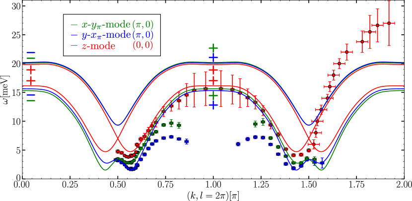
Figure 2: Computed best fit of the one-triplon dispersions for $J_{0}=$9.4\text{\,}\mathrm{m}\mathrm{e}\mathrm{V}$$, $J_{3}=$1.5\text{\,}\mathrm{m}\mathrm{e}\mathrm{V}$$, $J_{1}=1.2J_{0}$, $J_{2}=1.09J_{0}$, $D_{1}^{x}=0.58J_{0}$, $D_{1}^{y}=0.73J_{0}$, $D_{2,a}^{z}=-0.02J_{0}$, and $D_{3}^{y}=0.02J_{0}$. Components not listed are zero. The symbols with error bars show the inelastic neutron scattering data from Ref. plumb16 . The legend denotes the Zak phases of the modes in $k$- and $l$-direction, see main text. The plus and minus signs at the time reversal invariant wave numbers $0$ and $\pi$ indicate the parities of the modes.

For the model (4) with the appropriate fit parameters, see Fig. 2, we calculate the topological properties of the triplons where we treat them as non-interacting bosons. This appears to be a severe approximation, but it is not since the deepCUT dealt with the hardcore properties in the isotropic ladders rigorously, i.e. without any approximation. Only the weaker interladder couplings and the anisotropic couplings are approximated by the assumption of non-interacting bosons. For low energies and low temperatures, this is justified.

To assess the topological properties of bosonic bands one needs to generalise the Berry curvature to bosonic systems. Even for non-interacting bosons this is not trivial. For fermions the scalar product of quantum states can be naturally transferred to fermionic operators in second quantisation and the fermionic Bogoliubov transformations are unitary. But this does not hold for bosonic Bogoliubov transformations blaiz86 because the bosonic operators must be normalised with respect to a symplectic product, for details see Supplementary Material. The operator (7) is defined by its prefactors which we combine into a vector that we denote as a generalised ket state

$$\ket{\mathbf{k},n}\rangle:=(\mathbf{u}_{n,k,l}^{\top},\tilde{\mathbf{u}}_{n,k,l}^{\top},\mathbf{v}_{n,k,l}^{\top},\tilde{\mathbf{v}}_{n,k,l}^{\top})^{\top},$$ (8)

which is a column vector with twelve components. The bold face symbols such as $\mathbf{u}$ stand for three-dimensional column vectors with the components $u^{x},u^{y}$ and $u^{z}$. The symplectic product reads

$$\langle\bra{\mathbf{k}_{1},n_{1}}{\mathbf{k}_{2},n_{2}}\rangle\rangle:=$$

$$\qquad(\mathbf{u}_{n_{1},k_{1},l_{1}}^{\dagger},\tilde{\mathbf{u}}_{n_{1},k_{1},l_{1}}^{\dagger},\mathbf{v}_{n_{1},k_{1},l_{1}}^{\dagger},\tilde{\mathbf{v}}_{n_{2},k_{2},l_{2}}^{\dagger})\ \eta\ (\mathbf{u}_{n_{2},k_{2},l_{2}}^{\top},\tilde{\mathbf{u}}_{n_{2},k_{2},l_{2}}^{\top},\mathbf{v}_{n_{2},k_{2},l_{2}}^{\top},\tilde{\mathbf{v}}_{n_{2},k_{2},l_{2}}^{\top})^{\top}$$ (9a)

$$\qquad=\mathbf{u}_{n_{1},k_{1},l_{1}}^{\dagger}\mathbf{u}_{n_{2},k_{2},l_{2}}+\tilde{\mathbf{u}}_{n_{1},k_{1},l_{1}}^{\dagger}\tilde{\mathbf{u}}_{n_{2},k_{2},l_{2}}-\mathbf{v}_{n_{1},k_{1},l_{1}}^{\dagger}\mathbf{v}_{n_{2},k_{2},l_{2}}-\tilde{\mathbf{v}}_{n_{1},k_{1},l_{1}}^{\dagger}\tilde{\mathbf{v}}_{n_{2},k_{2},l_{2}}.$$ (9b)

We highlight the so far unnoted fact that $\widetilde{\mathcal{M}}_{k,l}$, but not $\mathcal{M}_{k,l}$, is self-adjoint with respect to this symplectic product implying the well-known facts that the eigen values are real and that creation and annihilation operators of different eigen values have to commute.

With the above definitions, the standard relations berne13 for the Berry connection

$$\mathbf{\mathcal{A}}_{n,\mathrm{sym}}(\mathbf{k})=\mathbf{i}\langle\bra{\mathbf{k},n}{\nabla}_{\mathbf{k}}\ket{\mathbf{k},n}\rangle$$ (10)

and the Berry phase

$$\Omega_{n}=\oint\mathbf{\mathcal{A}}_{n}(\mathbf{k})\mathrm{d}\mathbf{k}=\mathbf{i}\oint\langle\bra{\mathbf{k},n}\nabla_{\mathbf{k}}\ket{\mathbf{k},n}\rangle\mathrm{d}\mathbf{k}$$ (11)

can be kept. If the closed path in the above equation encompasses the Brillouin zone, $\Omega_{n}/(2\pi)$ renders the Chern number. We computed the Chern number of BiCu2PO6 , but it remains trivial even if magnetic fields are included which do not close the spin gap between the ground state and the lowest triplon mode. But there are other relevant topological phases in (quasi-)one-dimensional systems, notably the Zak phase zak89 ; delpl11 and the winding number joshi17 .

The Zak phase is a Berry phase computed along a closed loop in one direction in the Brillouin zone zak89 . Due to the periodicity in $k$-and $l$-space the closed loops $k\to k+2\pi$ or $l\to l+2\pi$ allow us to define two Berry phases, setting the lattice constants to unity. Each of these Berry phases can be averaged over the corresponding other momentum and combined into a vector $\mathbf{P}$ liu17 , which is defined by

$$\mathbf{P}=\frac{1}{2\pi}\int\mathbf{\mathcal{A}}_{n,\mathrm{sym}}\,\mathrm{d}k\,\mathrm{d}l\,.$$ (12)

The value of this vector for each triplon band is given in the legend of Fig. 2. The $z$-mode remains topologically trivial while the coupled $x$-$y_{\pi}$- and $x_{\pi}$-$y$-mode display the Zak phase $(\pi,0)$, for computational technicalities see Supplementary Material.

The above mentioned average does not matter in BiCu2PO6 because the Zak phase does not depend on the wave number $l$. The $l$-dependence in the investigated minimal model mainly enters via the isotropic term $J_{3}\cos(2\pi l)$, which does not alter the eigen modes since this term is proportional to unity. The small $D_{3}^{y}$ and the even smaller $\Gamma_{3}^{\alpha\alpha}$ barely have an impact on the dispersion and the eigen modes so that they do not influence the topology. The Zak phase is constant for all values of $l$ being either zero or $\pi$. It is pinned to these particular values in BiCu2PO6 because it is inversion symmetric, see Fig. 1(c). The transformation operator of inversion is given by the matrix $\Pi=\mathrm{diag}(1,1,1,-1,-1,-1,1,1,1,-1,-1,-1)$ with $\Pi^{2}=\mathds{1}$ which transforms $\Pi\mathcal{M}_{k,l}\Pi=\mathcal{M}_{-k,-l}$ and hence ensures the quantisation of the Zak phase. We stress that the Zak phase is robust, i.e. small changes of the model do not alter it. For instance, it remains the same if we pass from the minimal model to the extended model accounting for different copper sites. Similarly, one may reduce the values of $D_{1}^{x}$ and $D_{1}^{y}$ even by a factor 2, cf. Ref. plumb16 , and still retrieves the same Zak phase. We stress, however, that they must be different $D_{1}^{x}\neq D_{1}^{y}$ to keep the Zak phase. If they are equal, the topological bands are no longer separated so that no Zak phase can be defined or it is trivial. Note that $D_{1}^{x}\neq D_{1}^{y}$ is required in order to fit the experimental data. Furthermore, the Zak phase persists in the presence of magnetic fields which do not close the spin gap above the ground state. This insensitivity results from the fact that the twist in the $U(1)$ principal fiber bundle is generated by the coupling between the $k$ and $k+\pi$ momenta. Thus, terms coupling at the same momentum such as the magnetic field barely destruct the Zak phase.

The momenta with $k,l\in\{0,\pi\}$ are invariant under inversion so that the bands at these momenta have a sharply defined parities with respect to inversion denoted by “+” and by “–” in Fig. 2. The products of the parities at $k=0$ and $k=\pi$ both at $l=2\pi$ is equal to the exponential of the Zak phase hughe11 . This agrees with the direct computation of the Zak phase in $k$-direction. This represents an alternative way to determine Zak phases.

Another quantised topological index related to the Zak phase is the winding number schny08 ; delpl11 ; li15b ; joshi17 , which counts the number of windings around a point on a 2D plane. For this concept to make sense the Hamiltonian must have an additional symmetry, conventionally called chiral symmetry, so that its variation along the considered path of a control variable, here from $k=0$ to $k=2\pi$, can be described in a 2D plane, see Refs. delpl11 ; li15b ; joshi17 . Such a chiral symmetry can be found for the minimal model of BiCu2PO6 , i.e. ignoring the difference between the copper sites, while we were not able to find a chiral symmetry for the extended model accounting for different copper sites. The winding numbers $w$ found for the $x$-$y_{\pi}$- and $x_{\pi}$-$y$-mode both take the non-trivial value $w=1$, for details see Supplementary Material. We emphasise, however, that the Zak phase itself is by far a more general concept because its definition and computation does not require an additional chiral symmetry.

Generically, the bulk-boundary correspondence berne13 implies that there must exist additional states in spatially restricted geometries of topologically non-trivial phases. This holds if the topological invariant is quantised so that it cannot smoothly evolve towards a trivial value on the other side of the boundary. Edge states must exist in the gaps of strips of systems with finite Zak phase or finite winding number delpl11 ; li15b ; joshi17 . Hence we expected this to hold true in BiCu2PO6 and computed the energy spectra for finite pieces of the spin ladder pertaining to BiCu2PO6 . To our surprise we did not find any localised edge states. We studied the states quantitatively by computing the inverse participation ratio (IPR) krame93 which is the standard measure of (non-)localised states. If the IPR tends to zero for increasing system size the state is extended; if it stays finite the corresponding state is localised. Here we use the definition

$$I_{n}=\sum_{i}p_{n,i}^{2}=\sum_{i}|\langle\bra{n,i}{n,i}\rangle\rangle|^{2}$$ (13)

adapted to the bosonic symplectic product and found that $I_{n}\to 0$ for longer and longer spin ladders of BiCu2PO6 .

This puzzling fact appears to be at odds with the common lore on edge modes. But we can explain it by three arguments. First, the usual argument of bulk-boundary correspondence berne13 requires the existence of states within the band gaps of the topologically non-trivial bulk systems. But there is no argument which requires that these states are localised. The localisation is plausible because the states lie energetically within a gap and should not exist in the bulk far away from the boundaries. But if there is no gap the situation is not clear a priori.

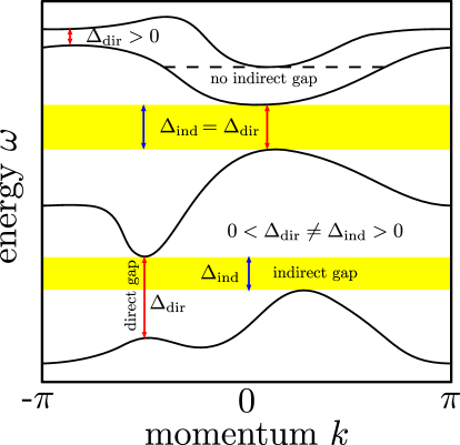
Figure 3: Illustration of a direct gap $\Delta_{\mathrm{dir}}$ at the red arrows and of an indirect gap $\Delta_{\mathrm{ind}}$ (blue arrows) by the forbidden yellow area. A direct gap is the minimal difference between the maximal energy of a lower mode and the minimal energy of an upper mode at the same momentum. In contrast, the indirect gap is given by a forbidden energy interval between both modes irrespective of momentum conservation.

Second, in most cases with localised edge states they lie in an indirect gap, i.e. there is a whole energy interval in the bulk without allowed states. The notion of direct and indirect gaps is common in semiconductor physics; it is illustrated in Fig. 3. If there is an indirect gap the gap persists even if we sum over all momenta as one has to do in computing local densities of states. We stress that introducing boundaries, for instance in $y$-direction, lifts the conservation of momentum $\hbar k$ so that generically all these momenta hybridise. (There may be exceptions to this hybridisation verre18a .) Since the corresponding hybridising states are extended plane waves, it is natural to expect that the resulting states are extended as well. This is what happens in BiCu2PO6 where the bands are separated by direct gaps, but not by indirect gaps.

The third argument resides in the independence of the topological invariants in the bulk on the energies. The vector potential (10) and hence the Berry phase (11) depend on the eigen modes only. They do not depend on their energies so that they are blind to their eigen energies, i.e. to the dispersions. Thus, one can modify the Hamiltonian leaving the eigen modes completely untouched, but shifting their energies arbitrarily. By construction, this does not alter the topological quantities. But it changes the system and has an effect on the edge modes if boundaries are introduced. To corroborate this consideration we studied the commonly considered Su-Schrieffer-Heeger model su79 , see Supplementary Material. In this transparent model, we show explicitly that adding a coupling, which does not alter the eigen states, does alter the localisation of the edge modes. If the indirect gap vanishes the edge modes cease to be localised, i.e. they are no longer modes at the edge in the proper sense. This finding puts the bulk-boundary correspondence generally into perspective.

To summarise, we analysed the available inelastic neutron scattering data in the framework of a magnetic valence bond crystal with triplons as elementary excitations. Within the resulting model, we computed the Zak phase as generic one-dimensional topological invariant; it takes the non-trivial value $\pi$. Due to inversion symmetry it has to be quantised in multiples of $\pi$. The non-trivial value is robust against not too large changes of the DM couplings. They may even vary by a factor of two, but it is important that $D_{1}^{x}\neq D_{1}^{y}$ holds. The topological character of BiCu2PO6 is supported by the winding number $w=-1$ based on the chiral symmetry of the minimal model.

Remarkably, we found that in spite of the topological bulk properties no localised edge modes occur. We clarified this unexpected finding by the distinction of direct and indirect gaps. Only the existence of an indirect gap warrants the localisation of edge modes. We point out that the standard bulk-boundary correspondence implies the existence of modes within the gaps separating the topological non-trivial bands, but it does not imply localisation. This has been corroborated by a comprehensive study of the paradigmatic Su-Schrieffer-Heeger model.

Our results identify BiCu2PO6 as the first disordered quantum antiferromagnet with finite quantized Zak phase and the second disordered antiferromagnet with topologically non-trivial eigen modes. So far, only SrCu2(BO3)2 had been known for its non-trivial triplon excitations. Further search for low-dimensional disordered quantum magnets with finite Zak phases or finite Chern numbers is to be expected. On the conceptual level, the scenario of delocalisation of edge modes deserves further investigation in all conceivable physical realisations.

• We acknowledge useful discussions with Christoph H. Redder and Joachim Stolze and provision of the experimental data by Kemp Plumb and Young-June Kim. Financial support (MM) was given by the Studienstiftung des Deutschen Volkes and by the Deutsche Forschungsgemeinschaft and the Russian Foundation of Basic Research through the transregio TRR 160.

• Competing Interests: The authors declare that they have no competing financial interests.

• Correspondence: Correspondence and requests for materials should be addressed to M.M. (email: maik.malki@tu-dortmund.de).

Supplementary Note 1: Symmetry analysis of BiCu2PO6

The direction of the Dzyaloshinskii-Moriya (DM) vectors $\mathbf{D}_{m},m\in\{0,1,2,3\}$ are restricted due to the symmetries of the system. These restrictions are formulated by the five selection rules of Moriya s_moriy60b which relate the different couplings based on the point group symmetries of the system. For the sake of completeness, we present these five selection rules here briefly. Moriya established them by considering two interacting ions with spins whose positions we label with $A$ and $B$. The center of the connecting line $\overline{AB}$ is denoted by $C$.

• If $C$ presents a center of inversion, then $\mathbf{D}=0$ holds.

• If there is a mirror plane perpendicular to $\overline{AB}$ and passing through $C$, then $\mathbf{D}\perp\overline{AB}$ is valid.

• If a mirror plane including the positions $A$ and $B$ is present, the vector $\mathbf{D}$ is perpendicular to this mirror plane.

• In case of a two-fold rotation axis perpendicular to the line $\overline{AB}$ and passing through $C$, then $\mathbf{D}$ is perpendicular to this two-fold rotation axis.

• If there is an $n$-fold axis ($n\geq 2$) passing along $\overline{AB}$, the relation $\mathbf{D}\parallel\overline{AB}$ is valid.

Besides the information that specific $\mathbf{D}_{ij}$ components are forbidden due to point group symmetries of the single bonds one can additionally obtain information on the signs of the possible $\mathbf{D}_{ij}$ along the ladder by considering translations and glide reflections. Likewise the parity of the components relative to reflection about the center line, see Fig. 1(c) in the main article, can be elucidated. This parity determines whether a term contributes to the dispersions on the level of bilinear Hamiltonians or not s_schmi05b .

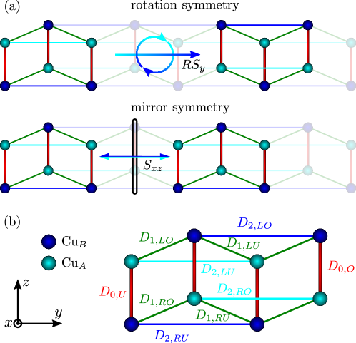
Figure S1: Symmetry analysis. (a) Illustration of the two symmetry operations $RS_{y}$ and $S_{xz}$ leaving the model of BiCu2PO6 invariant. (b) Notation of the various $\mathbf{D}$ vectors in BiCu2PO6 .

If we neglect the difference between the two copper ions Cu_A and Cu_B we arrive at the minimal model of BiCu2PO6 with the possible DM components shown in Fig. 1(c) of the main article. Taking into account the difference between the two copper sites s_tsirl10 the symmetry of the lattice is lower so that more $\mathbf{D}_{ij}$ components are allowed. Then only the following two symmetries of the crystal structure are present:

1. $RS_{y}$: Rotation by $\pi$ around the $y$-axis located in the middle of the spin ladder and a shift by half a unit cell.

2. $S_{xz}$: Reflection at the $xz$-plane located at a dimer.

These two symmetry operations are shown in Fig. S1(a). In Fig. S1(b) the notation of the various DM vectors is shown.

The determined symmetries imply the following constraints. The vector $\mathbf{D}_{0}$ only has a $y$-component due to the third selection rule based on the symmetry $S_{xz}$. The $RS_{y}$ symmetry yields the relation

$$RS_{y}(\mathbf{D}_{0,U})=-\mathbf{D}_{0,O}.$$ (S1)

After a $RS_{y}$ rotation the stipulated sequence of the spin operators within the term $\mathbf{D}_{ij}(\mathbf{S}_{i}\times\mathbf{S}_{j})$ (according to ascending $y$- and $z$-coordinate) must be recovered by swapping the spin operators. Thus, Eq. (S1) shows the alternating behaviour of $D_{0}^{y}$ along the legs. The symmetry analysis of the $\mathbf{D}_{1}$ bond leads to the relations

$$S_{xz}(\mathbf{D}_{1,LU}) =\mathbf{D}_{1,LO}$$ (S2a)

$$S_{xz}(\mathbf{D}_{1,LO}) =\mathbf{D}_{1,LU}$$ (S2b)

$$S_{xz}(\mathbf{D}_{1,RU}) =\mathbf{D}_{1,RO}$$ (S2c)

$$S_{xz}(\mathbf{D}_{1,RO}) =\mathbf{D}_{1,RU}$$ (S2d)

$$RS_{y}(\mathbf{D}_{1,LU}) =\mathbf{D}_{1,RO}$$ (S2e)

$$RS_{y}(\mathbf{D}_{1,LO}) =\mathbf{D}_{1,RU}$$ (S2f)

$$RS_{y}(\mathbf{D}_{1,RU}) =\mathbf{D}_{1,LO}$$ (S2g)

$$RS_{y}(\mathbf{D}_{1,RO}) =\mathbf{D}_{1,LU}.$$ (S2h)

To clarify the properties of $\mathbf{D}_{1}$ we start with an arbitrary vector

$$\mathbf{D}_{1,LU}=c_{x}\mathbf{e}_{x}+c_{y}\mathbf{e}_{y}+c_{z}\mathbf{e}_{z}$$ (S3)

where $\mathbf{e}_{\mu}$ are unit vectors in the directions indicated by the subscript and $c_{\mu}$ are real coefficients. Applying Eqs. (S2a) and (S2e) to this ansatz for $\mathbf{D}_{1,LU}$ we obtain

$$\mathbf{D}_{1,LO} =\phantom{-}c_{x}\mathbf{e}_{x}-c_{y}\mathbf{e}_{y}+c_{z}\mathbf{e}_{z}$$ (S4a)

$$\mathbf{D}_{1,RO} =-c_{x}\mathbf{e}_{x}+c_{y}\mathbf{e}_{y}-c_{z}\mathbf{e}_{z}.$$ (S4b)

The first condition determines that the $x$- and $z$-component are uniform while the $y$-component is alternating along the ladder. The second condition indicates that all three components have odd parity since the translation to $\mathbf{D}_{1,RU}$ changes the sign of the $y$-component as well so that all coefficients acquire a negative sign.

In the same way, we investigate $\mathbf{D}_{2}$. Applying both symmetry operations to $\mathbf{D}_{2}$ yields

$$S_{xz}(\mathbf{D}_{2,LU}) =\mathbf{D}_{2,LU}$$ (S5a)

$$S_{xz}(\mathbf{D}_{2,LO}) =\mathbf{D}_{2,LO}$$ (S5b)

$$S_{xz}(\mathbf{D}_{2,RU}) =\mathbf{D}_{2,RU}$$ (S5c)

$$S_{xz}(\mathbf{D}_{2,RO}) =\mathbf{D}_{2,RO}$$ (S5d)

$$RS_{y}(\mathbf{D}_{2,LU}) =\mathbf{D}_{2,RO}$$ (S5e)

$$RS_{y}(\mathbf{D}_{2,LO}) =\mathbf{D}_{2,RU}$$ (S5f)

$$RS_{y}(\mathbf{D}_{2,RU}) =\mathbf{D}_{2,LO}$$ (S5g)

$$RS_{y}(\mathbf{D}_{2,RO}) =\mathbf{D}_{2,LU}\,.$$ (S5h)

Again, we start from the general ansatz

$$\mathbf{D}_{2,LU}=d_{x}\mathbf{e}_{x}+d_{y}\mathbf{e}_{y}+d_{z}\mathbf{e}_{z}\,.$$ (S6)

Using Eq. (S5a) we easily see that the $y$-component has to vanish. In contrast, using Eq. (S5e) does not lead to an unambiguous solution because we obtain

$$\mathbf{D}_{2,RO}=-d_{x}\mathbf{e}_{x}-d_{z}\mathbf{e}_{z}\,.$$ (S7)

Each component can fulfil this condition in two different ways. Either the component is alternating along the ladder with even parity or it is uniform along the ladder with odd parity. Thus, the $\mathbf{D}_{2}$-vector is generally expressed by the superposition of both possibilities

$$D_{2}^{x} =D_{2,a}^{x}+D_{2,u}^{x}$$ (S8a)

$$D_{2}^{z} =D_{2,a}^{z}+D_{2,u}^{z}$$ (S8b)

where subscript $a$ stands for “alternating” and $u$ for “uniform”.

Considering the fact that the differences between the copper ions are small s_tsirl10 we may neglect them altogether which allows us to conclude s_splin16 $D_{2}^{x}=D_{2,u}^{x}$ and $D_{2}^{z}=D_{2,a}^{z}$. Thus, we conclude that the uniform $x$-component and the alternating $z$-component predominate. Arbitrary components as in Eq. (S8) are allowed, but decisive contributions only come from the alternating even parity $z$-component and the uniform odd parity $x$-component.

Note that we neglect potential differences between $\mathbf{D}_{2}$ on the $J_{2}$ bond and $\mathbf{D}^{\prime}_{2}$ on the $J_{2}^{\prime}$ bond because they have odd parity and do not contribute on the bilinear level anyway. The potential differences in the ensuing symmetric $\Gamma$-terms are neglected as well because of their barely measurable impact.

The results of the symmetry analysis are collected in Tab. 1. Since the $\Gamma$-couplings result from the $D$-couplings according to Eq. (3) in the main article one can establish a similar table for the $\Gamma$-components based on Tab. 1. The property of being alternating/odd corresponds to a minus sign while uniform/even to a plus sign in the DM components. Thus by multiplying $\pm 1$ to the DM components in Eq. (3) one arrives at the resulting properties of the $\Gamma$-components.

Finally, we remark that the orientation of the $\mathbf{D}_{3}$-vector, which belongs to the interladder coupling, is analogous to the $\mathbf{D}_{0}$-vector. The $\mathbf{D}_{3}$-vector couples two adjacent ladders contributing to the transversal dispersion. No parity can be defined because the reflection about the center line refers to a symmetry within each ladder separately.

Table 1: Behaviour of the sign of the $D$-components along the legs of the spin ladder and their parity with respect to the symmetry $S_{xy}$ (reflection with respect to the center line of the spin ladder, see Fig. 1(c) of the main text). $D$-components which are not listed are forbidden due to the selection rules of Moriya s_moriy60b .

couplings	along the legs	parity
$D_{0}^{y}$	alternating	odd
$D_{1}^{x}$	uniform	odd
$D_{1}^{y}$	alternating	odd
$D_{1}^{z}$	uniform	odd
$D_{2,a}^{x}$	alternating	even
$D_{2,u}^{x}$	uniform	odd
$D_{2,a}^{z}$	alternating	even
$D_{2,u}^{z}$	uniform	odd
$D_{3}^{y}$	alternating	N/A

Supplementary Note 2: Matrix representation of the bilinear Hamilton operator

The general expression in Nambu representation of the complete bilinear Hamiltonian in quasi-momentum space is given up to unimportant constants by

$$\mathcal{H}=\frac{1}{2}\sum_{k,l}\mathbf{a}_{k,l}^{\dagger}\mathcal{M}_{k,l}\mathbf{a}_{k,l}\quad\mathrm{with}\quad\mathcal{M}_{k,l}=\begin{bmatrix}A(k,l)&B(k,l)\\ B^{\dagger}(k,l)&A^{\top}(-k,-l)\end{bmatrix}=\mathcal{M}^{\dagger}_{k,l}$$ (S9)

and the twelve-dimensional Nambu spinor $\mathbf{a}_{k,l}=(\mathbf{t}_{k,l}^{\top},\mathbf{t}_{k+\pi,l}^{\top},\mathbf{t}_{-k,-l}^{\dagger},\mathbf{t}_{-k-\pi,-l}^{\dagger})^{\top}$, see Eq. (5) in the main text, using $\mathbf{t}_{k,l}=(t^{x}_{k,l},t^{y}_{k,l},t^{z}_{k,l})^{\top}$. Note that the sum in (S9) runs over all values of $l\in[0,2\pi)$ (lattice constant set to unity) in the Brillouin zone while it runs only over the values $k\in[0,\pi)$, i.e. over half the Brillouin zone. The reason is that the above Nambu spinor addresses $k$ and $k+\pi$ simultaneously.

The $12\times 12$ matrix $\mathcal{M}_{k,l}$ is composed of the two $6\times 6$ matrices $A$ and $B$ which are again made up by $3\times 3$ matrices

$$A(k,l) =\begin{pmatrix}A_{1}(k)+B_{1}(k,l)&B_{2}(k,l)\\ B_{2}^{\dagger}(k,l)&A_{1}(k+\pi)+B_{1}(k+\pi,l)\end{pmatrix}$$ (S10a)

$$B(k,l) =\begin{pmatrix}B_{1}(k,l)&B_{2}(k,l)\\ B_{2}^{\dagger}(k,l)&B_{1}(k+\pi,l)\,.\end{pmatrix}$$ (S10b)

The $3\times 3$ matrices are derived to be

$$A_{1}(k) =\begin{pmatrix}\omega_{0}(k)&\mathrm{i}h_{z}&-\mathrm{i}h_{y}\\ -\mathrm{i}h_{z}&\omega_{0}(k)&\mathrm{i}h_{x}\\ \mathrm{i}h_{y}&-\mathrm{i}h_{x}&\omega_{0}(k)\\ \end{pmatrix}$$ (S11a)

$$B_{1}(k,l) =\begin{pmatrix}F^{x}(k,l)&0&\Gamma_{1}^{xz}(k)+\Gamma_{2}^{xz}(k)\\ 0&F^{y}(k,l)&0\\ \Gamma_{1}^{xz}(k)+\Gamma_{2}^{xz}(k)&0&F^{z}(k,l)\\ \end{pmatrix}$$ (S11b)

$$B_{2}(k,l) =\begin{pmatrix}0&-\mathrm{i}(\Gamma_{1}^{xy}(k)-D_{2}^{z}(k))&-\mathrm{i}D_{3}^{y}(k,l)\\ -\mathrm{i}(\Gamma_{1}^{xy}(k)+D_{2}^{z}(k))&0&-\mathrm{i}(\Gamma_{1}^{yz}(k)-D_{2}^{x}(k))\\ \mathrm{i}D_{3}^{y}(k,l)&-\mathrm{i}(\Gamma_{1}^{yz}(k)+D_{2}^{x}(k))&0\end{pmatrix}\,.$$ (S11c)

Table 2: The coefficients $\omega_{\delta}$ in order to describe the dispersion of the isotropic spin ladder as well as the prefactors $a_{\delta}$ to transform the spin operators are calculated by using the deepCUT method for the ratios $J_{1}/J_{0}=1.2$ and $J_{2}/J_{1}=0.9$. The values for higher $\delta$ are small enough to be neglected.

$\delta$	$\omega_{\delta}$	$a_{\delta}$
0	-1.549938420848800000	-0.387449110915571300
1	-0.358817770492231000	-0.051650017047999240
2	-0.524739087510573000	-0.080958848050941240
3	-0.209722209664048000	-0.037136148896873510
4	-0.160344853773972000	-0.021929139775116400
5	-0.096751624573842900	-0.017194624948628080
6	-0.010462389004026000	-0.004727305201296136
7	-0.034704357201939800	-0.010242082594554390
8	-0.000112462598212057	-0.001628782296091526
9	-0.013929738864778900	-0.004974925019692490
10	-0.006377074783529710	-0.002315960919757644
11	-0.004037422865249410	-0.001621270078823474
12	-0.004295595426250670	-0.001835116321222724
13	-0.000461321168694168

The dispersion of the isotropic spin ladder is calculated by deepCUT method s_splin16 ; s_krull12 yielding

$$\omega_{0}(k)=\sum_{\delta=0}^{13}\omega_{\delta}\cos(\delta k)\,.$$ (S12)

The coefficients $\omega_{\delta}$ are given in Tab. 2. Similarly, the transformation of the spin operators to triplon operators

$$S^{\mu}_{0,L}=-S^{\mu}_{0,R}=\sum_{\delta=-12}^{12}a_{|\delta|}(t^{\mu}_{\delta}+t^{\mu,{\dagger}}_{\delta})+\text{bilinear and higher terms}$$ (S13)

yields the amplitudes $a_{\delta}$ also given in Tab. 2. The spin operators are labelled with subscript left ($L$) and right ($R$) spin in a dimer referring to the two legs of each ladder. Bilinear or higher products of triplon operators are neglected in our approach to the transformation of the spin operator. The Fourier transform

$$a(k):=\sum_{\delta=-12}^{12}a_{|\delta|}\cos(\delta k)$$ (S14)

yields the momentum dependent amplitude $a(k)$ which appears generically in effective triplon Hamiltonians s_uhrig04 ; s_uhrig05a ; s_splin16 . The Hamiltonian also includes a general uniform magnetic field $\mathbf{h}=(h_{x},h_{y},h_{z})^{\top}$ given by $\mathcal{H}_{\text{Zeeman}}=-\mathbf{h}\sum_{i}\mathbf{S}_{i}$.

Further variables introduced for clarity are

$$F^{\mu}(k,l)=d(k,l)+\Gamma_{0}^{\mu\mu}(k)+\Gamma_{1}^{\mu\mu}(k)+\Gamma_{2}^{\mu\mu}(k)+\Gamma_{3}^{\mu\mu}(k,l)\quad\mathrm{with}\quad\mu\in\left\{x,y,z\right\}$$ (S15)

and

$$d(k,l) =-2J_{3}\cos(2\pi l)a^{2}(k)$$ (S16a)

$$\Gamma_{0}^{\mu\mu}(k) =-2\Gamma_{0}^{\mu\mu}a^{2}(k)$$ (S16b)

$$\Gamma_{1}^{\mu\mu}(k) =\phantom{-}4\Gamma_{1}^{\mu\mu}a^{2}(k)\cos(k)$$ (S16c)

$$\Gamma_{2}^{\mu\mu}(k) =\phantom{-}4\Gamma_{2}^{\mu\mu}a^{2}(k)\cos(2k)$$ (S16d)

$$\Gamma_{3}^{\mu\mu}(k,l) =-2\Gamma_{3}^{\mu\mu}a^{2}(k)\cos(2\pi l)$$ (S16e)

$$\Gamma_{1}^{xy}(k) =\phantom{-}4\Gamma_{1}^{xy}a(k)a(k+\pi)\sin(k)$$ (S16f)

$$\Gamma_{1}^{yz}(k) =\phantom{-}4\Gamma_{1}^{yz}a(k)a(k+\pi)\sin(k)$$ (S16g)

$$\Gamma_{1}^{xz}(k) =\phantom{-}4\Gamma_{1}^{xz}a(k)^{2}\cos(k)$$ (S16h)

$$\Gamma_{2}^{xz}(k) =\phantom{-}4\Gamma_{2}^{xz}a(k)^{2}\cos(2k)$$ (S16i)

$$D_{2,a}^{z}(k) =\phantom{-}4D_{2,a}^{z}a(k)a(k+\pi)\sin(2k)$$ (S16j)

$$D_{2,a}^{x}(k) =\phantom{-}4D_{2,a}^{x}a(k)a(k+\pi)\sin(2k)$$ (S16k)

$$D_{3}^{y}(k,l) =-2D_{3}^{y}a(k)a(k+\pi)\sin(2\pi l).$$ (S16l)

Inspecting the above matrices one realizes that for zero magnetic field the slightly simpler form

$$\mathcal{M}_{k,l}=\begin{bmatrix}A(k,l)&B(k,l)\\ B(k,l)&A(k,l)\end{bmatrix}$$ (S17)

holds.
 
 

Supplementary Note 3: Symplectic product and Berry phase for bosons

The Berry phase in quantum mechanics is defined by means of the complex phase of the scalar product between two quantum states s_berry84 . Thus, the key step is to define an appropriate scalar product.

In the main article, we use a symplectic product (9) for the coefficients of bosonic creation and annihilation operators. Note that this is a description on the level of second quantisation. Here we want to elucidate more of its formal properties. To be as general as possible, we consider a set of bosonic annihilation operators $a_{j}$ and creation operators $a^{\dagger}_{j}$ with $j\in\{1,2,\ldots m\}$. A general linear combination $c$ reads

$$c:=\sum_{j=1}^{m}(u_{j}a_{j}^{\dagger}-v_{j}a_{j})$$ (S18)

where $c$ is not normalized and it is not specified whether it is a creation or annihilation operator. Then, we define the corresponding generalized ket state by the column vector

$$|c\rangle\rangle:=(u_{1},\ldots,u_{m},v_{q},\ldots,v_{m})^{\top}=\underline{c}.$$ (S19)

Sometimes the vector notation $\underline{c}$ is more convenient than the ket notation. Axiomatically, we can define the symplectic product between two kets $|c\rangle\rangle$ and $|c^{\prime}\rangle\rangle$ by

$$\langle\langle c|c^{\prime}\rangle\rangle :=\sum_{j=1}^{m}(u^{*}_{j}u^{\prime}_{j}-v^{*}_{j}v^{\prime}_{j})$$ (S20a)

$$=\underline{c}^{\dagger}\eta\underline{c}^{\prime},$$ (S20b)

where the diagonal $2m\times 2m$ matrix $\eta=\text{diag}(1_{1},\ldots,1_{m},-1_{m+1},\ldots,-1_{2m})$ is used as a metric with $\eta^{2}=\mathds{1}$. This sort of “generalized scalar product” runs under several names in the literature such as “quasi-scalar product” or “para-scalar product” s_colpa78 ; s_kawag12 ; s_shind13 . We prefer to avoid the term “scalar product” which suggests semi-positivity, but use the established attribute “symplectic”. It is easy to verify that a conventional Hermitian matrix $M=M^{\dagger}$ is not self-adjoint with respect to Eqs. (S20). But $\eta M$ is self-adjoint due to

$$\langle\langle c|\eta Mc^{\prime}\rangle\rangle =\underline{c}^{\dagger}\eta\eta M\underline{c}^{\prime}$$ (S21a)

$$=\underline{c}^{\dagger}M\underline{c}^{\prime}$$ (S21b)

$$\langle\langle\eta Mc|c^{\prime}\rangle\rangle =\underline{c}^{\dagger}M\eta\eta\underline{c}^{\prime}$$ (S21c)

$$=\underline{c}^{\dagger}M\underline{c}^{\prime}.$$ (S21d)

Alternatively, one can also start from

$$\langle\langle c|c^{\prime}\rangle\rangle:=[c^{\dagger},c^{\prime}]$$ (S22)

which obviously yields an expression identical to Eqs. (S20). We observe that $\langle\langle c|c\rangle\rangle>0$ tells us that $c$ is an unnormalised creation operator while $\langle\langle c|c\rangle\rangle<0$ tells us that it is an unnormalised annihilation operator.

The following question is imminent at this stage: Can one relate Eqs. (S20) and Eq. (S22) to the conventional scalar product between quantum states? The answer is ambiguous: it depends. If there is a general ground state, i.e.  a vacuum $\ket{0}$ annihilated by all annihilation operators $b$ considered (here the linear combinations $b$ have to be annihilation operators), then the following relation between the standard scalar product $\bra{0}b^{\prime}b^{\dagger}\ket{0}$ in Fock space for two one-particle states and the above defined symplectic product holds

$$\bra{0}b^{\prime}b^{\dagger}\ket{0} =\bra{0}(b^{\prime}b^{\dagger}-b^{\dagger}b^{\prime})\ket{0}$$ (S23a)

$$=[b^{\prime},b^{\dagger}]$$ (S23b)

where the last line is precisely definition (S22) equivalent to (S20). Indeed, this situation is a very common one in multi-band systems where $\ket{0}$ is the vacuum with respect to all bosons at all values of $\mathbf{k}$. Then one retrieves the Berry connection (10) and the Berry phase (11) for paths through the Brillouin zone in the main text.

But we stress that the identity (S23) does not hold if an external control parameter $\lambda$ is varied which changes the vacuum as well. Then the Berry phase for a path from $\lambda=0$ to $\lambda=\lambda_{1}$ reads

$$\Omega =\mathbf{i}\int_{0}^{\lambda_{1}}\bra{0(\lambda)}b(\lambda)\partial_{\lambda}b^{\dagger}(\lambda)\ket{0(\lambda)}d\lambda$$ (S24a)

$$=\mathbf{i}\int_{0}^{\lambda_{1}}\left[\bra{0(\lambda)}b(\lambda)\left\{\partial_{\lambda}b^{\dagger}(\lambda)\right\}\ket{0(\lambda)}+\bra{0(\lambda)}b(\lambda)b^{\dagger}(\lambda)\left\{\partial_{\lambda}\ket{0(\lambda)}\right\}\right]d\lambda$$ (S24b)

$$=\mathbf{i}\int_{0}^{\lambda_{1}}\left[\bra{0(\lambda)}[b(\lambda),\left\{\partial_{\lambda}b^{\dagger}(\lambda)\right\}]\ket{0(\lambda)}+\bra{0(\lambda)}\left\{\partial_{\lambda}\ket{0(\lambda)}\right\}\right]d\lambda$$ (S24c)

$$=\Omega_{\text{exc}}(\lambda_{1})+\Omega_{\text{vac}}(\lambda_{1})$$ (S24d)

where two contributions are identified

$$\Omega_{\text{exc}}(\lambda_{1}) :=\mathbf{i}\int_{0}^{\lambda_{1}}\bra{0(\lambda)}[b(\lambda),\left\{\partial_{\lambda}b^{\dagger}(\lambda)\right\}]\ket{0(\lambda)}d\lambda$$ (S25a)

$$\Omega_{\text{vac}}(\lambda_{1}) :=\mathbf{i}\int_{0}^{\lambda_{1}}\bra{0(\lambda)}\left\{\partial_{\lambda}\ket{0(\lambda)}\right\}d\lambda.$$ (S25b)

One, $\Omega_{\text{exc}}$, results from the bosonic excitation and equals what one obtains using the symplectic product. The other, $\Omega_{\text{vac}}$, is the Berry phase of the vacuum. For paths in the Brillouin zone the analogous result has been derived in Ref. s_peano16 where, however, the vacuum contribution should not occur because the global vacuum of the system does not depend on momentum.

The bottom line is that for topological properties defined on the Brillouin zone the symplectic product yield a Berry phase identical to the conventional definition. In more general cases, however, the variation of the vacuum matters as well.

We corroborate this conclusion by repeating Berry’s original adiabatic approach in the bosonic Fock space. Let us assume that the bilinear Hamiltonian depends on the parameter $\lambda$ which may parametrises a path in the Brillouin zone or may be an external control parameter. It is varied slowly from $0$ to $1$, i.e. $\lambda=t/T$ for $t\in[0,T]$ with $T\to\infty$. The Hamiltonian is generally given by the matrix $\mathcal{M}(\lambda)$ s_blaiz86 ; for an example see Eq. (4) in the main article. At each value of $\lambda$ the ket $|n(\lambda)\rangle$ parametrises the creation of a boson in the $n$th eigen mode. Hence the equation

$$\eta\mathcal{M}(\lambda)\ket{n(\lambda)}\rangle=\omega_{n}(\lambda)\ket{n(\lambda)}\rangle$$ (S26)

is fulfilled. We assume the eigen modes to be non-degenerate for clarity. The adiabatic ansatz, see for instance Ref. s_uhrig91 , for the solution $\ket{\psi_{n}(t)}$ close to the instantaneous eigen state $\ket{\phi_{n}(\lambda)}:=b^{\dagger}_{n}(\lambda)\ket{0(\lambda)}$ reads

$$\ket{\psi_{n}(t)}=\exp(-i\Theta(t))\left(\ket{\phi_{n}(\lambda(t))}+(1/T)\ket{\perp}\right)$$ (S27)

where the correction $(1/T)\ket{\perp}$ is small in $1/T$ and perpendicular to $\ket{\phi_{n}(\lambda(t))}$. Inserting this ansatz in the Schrödinger equation $\mathbf{i}\partial_{t}\ket{\psi_{n}(t)}=H\ket{\psi_{n}(t)}$ yields

$$H\ket{\psi_{n}(t)}=(\partial_{t}\Theta)\ket{\psi_{n}(t)}+\exp(-i\Theta(t))\frac{\mathbf{i}}{T}\partial_{\lambda}\ket{\phi_{n}(\lambda)}+\text{perpendicular terms}.$$ (S28)

Next, we multiply with $\bra{\phi_{n}(\lambda)}$ from the left to obtain

$$\omega_{n}(\lambda)+E_{0}(\lambda)=\partial_{t}\Theta+\frac{1}{T}\partial_{\lambda}(\Omega_{\text{exc}}(\lambda)+\Omega_{\text{vac}}(\lambda))$$ (S29)

where $E_{0}$ is the ground state energy and we used the result of the calculation (S24). Integrating from $\Theta(t=0)=0$ to $t=T$ yields

$$\Theta(T)=T\int_{0}^{1}(\omega_{n}(\lambda)+E_{0}(\lambda))d\lambda-\Omega_{exc}(1)-\Omega_{vac}(1).$$ (S30)

This is the usual result for Berry phases in an adiabatic setting. The first term represents the dynamic phase and the second term $\Omega_{\text{exc}}(1)+\Omega_{\text{vac}}(1)$ is the Berry phase. Clearly, there is a contribution from the excitation and potentially from the ground state, i.e. the bosonic vacuum. Again, if the ground state is a global vacuum applying to all bosons it does not change as a function of $\lambda$. Then there is no vacuum Berry phase, i.e. $\Omega_{\text{vac}}=0$. This is the case for topological phases determined in the Brillouin zone.

Supplementary Note 4: Numerical calculation of the Zak phase

Only in rare cases, the analytical determination of the Zak phase is possible. In particular for higher dimensional problems, for instance the twelve dimensional extended model considered for BiCu2PO6 , a numerical approach is needed. The first step is to discretise the contour of integration. As an example for determining the phase from $k=0$ to $k=2\pi$ we use $k_{i}=\frac{2\pi i}{N}$ with $i=0,1,\cdots,N-1$ (lattice constant is set to unity). It is straightforward to determine the eigen modes $\ket{n,k_{i}}\rangle$ numerically. But the numerical choice of phase at each momentum $k_{i}$ is arbitrary so that we cannot rely on a continuous evolution and hence an approximation of

$$\Omega_{n}=\mathbf{i}\int_{0}^{2\pi}\langle\bra{n,k}\partial_{k}\ket{n,k}\rangle dk$$ (S31)

does not work. A well-established solution s_grusd14 ; s_wilcz84 consists in using the Wilson loop

$$\Omega_{n}=-\mathrm{Im}\sum_{i=0}^{N-1}\,\ln\left(\langle\braket{n,k_{i}}{n,k_{i+1}}\rangle\right)\quad\mathrm{mod}\;2\pi$$ (S32)

instead, where $\ket{n,k_{0}}\rangle=\ket{n,k_{N}}\rangle$ holds because the loop is closed. We stress that in the above formula the gauge, i.e. the choice of the phase, of each eigen mode does not matter because it cancels. Re-gauging each eigen mode arbitrarily

$$\ket{n,k_{j}}\rangle\to\widetilde{\ket{n,k_{j}}\rangle}=\exp(\mathbf{i}\varphi_{j})\ket{n,k_{j}}\rangle$$ (S33)

does not alter the outcome of Eq. (S32) because each eigen mode appears once as ket and once as bra.

An alternative variant of the above approach relies on the idea of parallel transport. The eigen mode $\ket{n,k_{j}}\rangle$ serves as reference state for $\ket{n,k_{j+1}}\rangle$. If their symplectic product reads

$$\langle\braket{n,k_{j}}{n,k_{j+1}}\rangle=z=|z|\exp(-\mathbf{i}\varphi_{j+1})$$ (S34)

we re-gauge $\ket{n,k_{j+1}}\rangle$ such that it becomes as parallel as possible to $\ket{n,k_{j}}\rangle$. Obviously, this is achieved by

$$\ket{n,k_{j+1}}\rangle\to\widetilde{\ket{n,k_{j+1}}\rangle}=\exp(\mathbf{i}\varphi_{j+1})\ket{n,k_{j+1}}\rangle.$$ (S35)

This procedure is iterated recursively from $j=0$ to $j=N-2$. The next and final step for $j=N-1$ yields $\varphi_{N}$, but the corresponding re-gauging (S35) is not possible because the phase of $\ket{n,k_{0}}\rangle=\ket{n,k_{N}}\rangle$ is fixed already. Then the total sum (S32) simply reduces to

$$\Omega_{n}=-\mathrm{Im}\ln\left(\langle\braket{n,k_{N-1}}{n,k_{0}}\rangle\right),$$ (S36)

since all re-gauged products are real and positive and the Zak phase corresponds to

$$\Omega_{n}=\varphi_{N}.$$ (S37)

The attractive feature of this second variant is that it reveals the geometric character of the Berry phases. They stem from the parallel transport in the U(1) principal fiber bundle of the manifold given by the eigen modes as functions of momenta.

Supplementary Note 5: Winding number $w$

In the case of the established minimal model for BiCu2PO6 the Hamiltonian shows an additional, chiral symmetry which allows us to calculate the winding number even in the presence of Bogoliubov terms. Here we show the details of the calculation of the winding number.

In the minimal model with $D_{3}^{y}=0$, the $12\times 12$ matrix in Eq. (6) in the main article or in Eq. (S9) in Note 2 can be split into $4\times 4$ matrices simplifying the subsequent analysis which is performed similarly to the one in Ref. s_joshi17 . To this end, we focus on the $x$-mode and its coupling to the $y_{\pi}$-mode. Since all couplings which are proportional to the $4\times 4$ identity matrix do not alter the eigen modes they do not alter the topological properties and are therefore neglected. The coupling contributions proportional to $\sigma_{x}\otimes\mathds{1}$ only lead to small variations of the energy dispersion and we neglect them in a simplifying approximation. We checked that their omission has no impact on the Zak phase. We expect that the winding number similarly is not changed by the couplings proportional to $\sigma_{x}\otimes 1$. The same is assumed for the inclusion of small $D_{3}^{y}$. Thus, for simplicity, we consider the Hamiltonian of single ladders

$$\mathcal{H}=\frac{1}{2}\sum_{k}\mathbf{a}_{k}^{\dagger}\mathcal{M}_{k}\mathbf{a}_{k}$$ (S38)

with the Nambu spinor $\mathbf{a}_{k}=(t_{k}^{x},t_{k+\pi}^{y},t_{-k}^{x,\dagger},t_{-k-\pi}^{y,\dagger})^{\top}$ and the $4\times 4$ matrix

$$\mathcal{M}_{k}=\begin{bmatrix}C(k)&C(k)\\ C(k)&C(k)\end{bmatrix},$$ (S39)

where the $2\times 2$ matrix $C$ is parametrised by Pauli matrices $\mathbf{\sigma}=\left(\sigma_{x},\sigma_{y},\sigma_{z}\right)$

$$C(k) =\mathbf{d}(k)\cdot\mathbf{\sigma}$$ (S40a)

$$\mathbf{d}(k) =\left(0,\Gamma_{1}^{xy}(k)-D_{2}^{z}(k),\frac{1}{2}\sum_{i=0}^{2}(\Gamma_{i}^{xx}(k)-\Gamma_{i}^{yy}(k+\pi))\right).$$ (S40b)

Then, the chiral symmetry operator is easy to identify as $\mathds{1}\otimes\sigma_{x}$. It fulfils the anticommutator $\left\{\mathds{1}\otimes\sigma_{x},\mathcal{M}_{k}\right\}=0$. In order to calculate the winding number we transform the Hamiltonian into the eigen basis of the chiral symmetry operator. This is achieved by the unitary transformation

$$U=\frac{1}{\sqrt{2}}\begin{pmatrix}1&0&1&0\\ 1&0&-1&0\\ 0&1&0&1\\ 0&1&0&-1\end{pmatrix}.$$ (S41)

In this basis, the Hamiltonian matrix $\eta\mathcal{M}_{k}$ with the metric $\eta=\sigma_{z}\otimes\mathds{1}$ has a block off-diagonal form

$$\widetilde{\mathcal{M}}_{k} =U^{\dagger}(\eta\mathcal{M}_{k})U$$ (S42a)

$$=\begin{bmatrix}0&D_{1}(k)\\ D^{*}_{1}(k)&0\end{bmatrix}.$$ (S42b)

The matrix $D_{1}(k)$ is given by

$$D_{1}(k)=\begin{pmatrix}d_{3}(k)+\mathbf{i}d_{2}(k)&d_{3}(k)+\mathbf{i}d_{2}(k)\\ -d_{3}(k)-\mathbf{i}d_{2}(k)&-d_{3}(k)-\mathbf{i}d_{2}(k)\\ \end{pmatrix}$$ (S43)

and the winding number s_joshi15 is calculated by

$$w=\frac{1}{8\pi\mathbf{i}}\oint_{\mathrm{BZ}}\mathrm{d}k\mathrm{Tr}_{2}\left(D^{-1}\partial_{k}D-(D^{\dagger})^{-1}\partial_{k}D^{\dagger}\right)$$ (S44)

with $D=\left(D_{1}(k)+D_{1}^{\top}(k)\right)/2$. By construction, the winding number is quantized to integer values $w\in\mathds{Z}$. For the investigated mode we find $w=-1$.

The same analysis can be performed for the $y$-mode coupled to the $x_{\pi}$-mode yielding the same winding number. In contrast, the $z$-mode only displays the trivial winding number $w=0$ because it does not couple with another mode. Hence, it cannot be twisted or wound in any way.

A chiral symmetry of the general $12\times 12$ matrix including all possible contributions could not be identified so that we could not define a winding number in general.  
 
 

Supplementary Note 6: (De)Localisation of the edge modes in the Su-Schrieffer-Heeger (SSH) model

In the main article, we provide three arguments why an edge state generically delocalises if the system does not display an indirect gap between the two bands where the eigen energy of the edge state is located. Since the topology of bosonic systems is still less known and the model for BiCu2PO6 is rather intricate we want to support our hypothesis on the delocalisation of edge states by a transparent calculation for an established and well-known fermionic model.

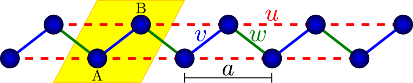
Figure S2: Lattice of the extended Su-Schrieffer-Heeger model with intracell coupling $v$, intercell couplings $w$ between nearest neighbour and intercell coupling $u$ between next-nearest neighbours. The unit cell comprising site $A$ and $B$ is displayed by the yellow area.

In order to do so we consider the SSH model s_su79 and extend it slightly by the coupling $u$ between next-nearest neighbours, see Fig. S2. Its Hamiltonian reads

$$\mathcal{H}_{\text{SSH}}=\sum_{i}^{N}v\left(c_{i,B}^{\dagger}c_{i,A}^{\phantom{\dagger}}+wc_{i+1,A}^{\dagger}c_{i,B}^{\phantom{\dagger}}+uc_{i+1,A}^{\dagger}c_{i,A}^{\phantom{\dagger}}+uc_{i+1,B}^{\dagger}c_{i,B}^{\phantom{\dagger}}\right)+\text{h.c.}$$ (S45)

where $c_{i,A}$ is the fermionic annihilation operator on site $A$ of unit cell $i$ and $c_{i,B}$ the corresponding fermionic annihilation operator on site $B$. The Hermitian conjugate operators are the creation operators. The three couplings are shown in Fig. S2. The Hamiltonian $\mathcal{H}_{\text{SSH}}$ is particle-conserving. In the bulk or for periodic boundary conditions a Fourier transformation yields

$$\mathcal{H} =\sum_{k}\begin{pmatrix}c_{k,A}^{\dagger}&c_{k,B}^{\dagger}\end{pmatrix}\mathcal{M}_{k}\begin{pmatrix}c_{k,A}^{\phantom{\dagger}}\\ c_{k,B}^{\phantom{\dagger}}\end{pmatrix}$$ (S46a)

$$\mathcal{M}_{k} =\begin{pmatrix}2u\cos(k)&v+w\mathrm{e}^{\mathrm{i}k}\\ v+w\mathrm{e}^{-\mathrm{i}k}&2u\cos(k)\end{pmatrix},$$ (S46b)

where the lattice constant $$a$$ is set to unity.

The ensuing dispersion is

$$\varepsilon_{n}(k)=2u\cos(k)\pm\sqrt{v^{2}+w^{2}+2vw\cos(k)}$$ (S47)

with $n\in\{1,2\}$ corresponding to the $\pm$ sign in front of the square root. The dispersion branches are depicted in the upper row of Fig. S3 for $v=0$ and the indicated ratios $u/w$.

On the one hand, the eigen states are the same as in the usual SSH model without next-nearest neighbour coupling $u$ since the additional coupling leads to a modification of the matrix $\mathcal{M}_{k}$ proportional to the $2\times 2$ identity matrix $2u\cos(k)\mathds{1}_{2}$. For this reason, we call the coupling $u$ isotropic. The induced modification does not change the eigen states. Hence, the extended SSH model shows the same Zak phase and the same winding number as the non-extended SSH model.

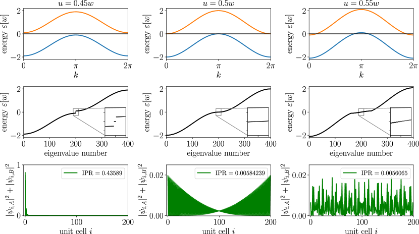
Figure S3: Delocalisation of the edge states illustrated for $v=0$. The three rows show from top to bottom: the bulk dispersion, the eigen values of a finite piece of chain with open boundaries consisting of 200 unit cells and the probability density $|\psi_{i,A}|^{2}+|\psi_{i,B}|^{2}$ of the eigen state $\psi$ with the highest inverse participation ratio (IPR) given in the legend of the lower panels. The three columns refer to different ratios $u/w$. For $u=0.45w$, the two edge modes lie within the indirect gap and are well localised. The case $u=0.5w$ is marginal and for $u=0.55w$ no indirect gap exists anymore. Concomitantly, no localised modes exist. But note that the two bands continue to be clearly separated.

On the other hand, however, the numerical analysis of a finite piece of chain with open boundary condition reveals that the localisation of the edge states is not protected against the isotropic coupling despite the fact that the direct gap does not close so that the two bands remain separated, see Fig. S3. By the naked eye one already discerns that the wave function with the largest value of the inverse participation ratio (IPR) defined in Eq. (13) in the main article, see also Ref. s_krame93 , is localised if the energy of the edge modes lies well within the indirect gap. But upon decreasing the indirect gap to zero for $u\to w/2$ the IPR drops to zero as well in the thermodynamic limit. Then it is obvious that the corresponding states are no longer localised. We emphasise that this does not contradict the argument of bulk-boundary correspondence which simply requires that the energy gap has to close at the boundary to another phase with a different quantized topological invariant.

This important result specifies the meaning of the wide-spread used bulk-boundary correspondence more precisely.

References

- (1) F. D. M. Haldane, Nobel lecture: Topological quantum matter, Rev. Mod. Phys. 89(4), 040502 (2017), doi:10.1103/RevModPhys.89.040502.
- (2) M. König, S. Wiedmann, C. Brüne, A. Roth, H. Buhmann, L. W. Molenkamp, X.-L. Qi and S.-C. Zhang, Quantum spin hall insulator state in hgte quantum wells, Science 318(5851), 766 (2007), doi:10.1126/science.1148047.
- (3) M. Z. Hasan and C. L. Kane, Topological insulators, Rev. Mod. Phys. 82(4), 3045 (2010), doi:10.1103/RevModPhys.82.3045.
- (4) X.-L. Qi and S.-C. Zhang, Topological insulators and superconductors, Rev. Mod. Phys. 83(4), 1058 (2011), doi:10.1103/RevModPhys.83.1057.
- (5) A. B. Bernevig and T. L. Hughes, Topological Insulators and Topological Superconductors, Princeton University Press, Princeton, doi:10.1515/9781400846733 (2013).
- (6) Y. Ando, Topological insulator materials, J. Phys. Soc. Jpn. 82(10), 102001 (2013), doi:10.7566/JPSJ.82.102001.
- (7) C.-Z. Chang, J. Zhang, X. Feng, J. Shen, Z. Zhang, M. Guo, K. Li, Y. Ou, P. Wei, L.-L. Wang, Z.-Q. Ji, Y. Feng et al., Experimental observation of the quantum anomalous hall effect in a magnetic topological insulator, Science 340(6129), 167 (2013), doi:10.1126/science.1234414.
- (8) N. Goldman, J. C. Budich and P. Zoller, Topological quantum matter with ultracold gases in optical lattices, Nat. Phys. 12(7), 639 (2016), doi:10.1038/nphys3803.
- (9) M. C. Rechtsman, J. M. Zeuner, Y. Plotnik, Y. Lumer, D. Podolsky, F. Dreisow, S. Nolte, M. Segev and A. Szameit, Photonic Floquet topological insulators, Nature 496(7444), 196 (2013), doi:10.1038/nature12066.
- (10) T. Jacqmin, I. Carusotto, I. Sagnes, M. Abbarchi, D. Solnyshkov, G. Malpuech, E. Galopin, A. Lemaître, J. Bloch and A. Amo, Direct observation of Dirac cones and a flatband in a honeycomb lattice for polaritons, Physical Review Letters 112(11), 116402 (2014), doi:10.1103/PhysRevLett.112.116402.
- (11) Z. Yang, F. Gao, X. Shi, X. Lin, Z. Gao, Y. Chong and B. Zhang, Topological acoustics, Physical Review Letters 114(11), 114301 (2015), doi:10.1103/PhysRevLett.114.114301.
- (12) C. Kane and T. Lubensky, Topological boundary modes in isostatic lattices, Nature Physics 10(1), 39 (2014), doi:10.1038/nphys2835.
- (13) R. Süsstrunk and S. D. Huber, Observation of phononic helical edge states in a mechanical topological insulator, Science 349(6243), 47 (2015), doi:10.1126/science.aab0239.
- (14) H. Katsura, N. Nagaosa and P. A. Lee, Theory of the thermal hall effect in quantum magnets, Phys. Rev. Lett. 104, 066403 (2010), doi:10.1103/PhysRevLett.104.066403.
- (15) Y. Onose, T. Ideue, H. Katsura, Y. Shiomi, N. Nagaosa and Y. Tokura, Observation of the magnon hall effect, Science 329, 297 (2010), doi:10.1126/science.1188260.
- (16) R. Matsumoto and S. Murakami, Theoretical prediction of a rotating magnon wave packet in ferromagnets, Phys. Rev. Lett. 106, 197202 (2011), doi:10.1103/PhysRevLett.106.197202.
- (17) R. Shindou, R. Matsumoto, S. Murakami and J.-I. Ohe, Topological chiral magnonic edge mode in a magnonic crystal, Phys. Rev. B 87(17), 174427 (2013), doi:10.1103/PhysRevB.87.174427.
- (18) L. Zhang, J. Ren, J.-S. Wang and B. Li, Topological magnon insulator in insulating ferromagnet, Phys. Rev. B 87, 144101 (2013), doi:10.1103/PhysRevB.87.144101.
- (19) R. Chisnell, J. S. Helton, D. E. Freedman, D. K. Singh, R. I. Bewley, D. G. Nocera and Y. S. Lee, Topological magnon bands in a kagome lattice ferromagnet, Phys. Rev. Lett. 115(14), 147201 (2015), doi:10.1103/PhysRevLett.115.147201.
- (20) J. Romhányi, K. Penc and R. Ganesh, Hall effect of triplons in a dimerized quantum magnet, Nat. Comm. 6, 6805 (2015), doi:10.1038/ncomms7805.
- (21) M. Malki and K. P. Schmidt, Magnetic chern bands and triplon hall effect in an extended shastry-sutherland model, Phys. Rev. B 95(19), 195137 (2017), doi:10.1103/PhysRevB.95.195137.
- (22) P. A. McClarty, F. Krüger, T. Guidi, S. F. Parker, K. Refson, A. Parker, D. Prabhakaran and R. Coldea, Topological triplon modes and bound states in a shastry–sutherland magnet, Nat. Phys. 13(8), 736 (2017), doi:10.1038/nphys4117.
- (23) K. W. Plumb, K. Hwang, Y. Qiu, L. W. Harriger, G. E. Granroth, A. I. Kolesnikov, G. J. Shu, F. C. Chou, C. Ruegg, Y. B. Kim and Y.-J. Kim, Quasiparticle-continuum level repulsion in a quantum magnet, Nat. Phys. 12(3) (2016), doi:10.1038/NPHYS3566.
- (24) L. Splinter, N. A. Drescher, H. Krull and G. S. Uhrig, Minimal model for the frustrated spin ladder system , Phys. Rev. B 94(15), 155115 (2016), doi:10.1103/PhysRevB.94.155115.
- (25) K. Hwang and Y. B. Kim, Theory of triplon dynamics in the quantum magnet bicupo, Phys. Rev. B 93(23), 235130 (2016), doi:10.1103/PhysRevB.93.235130.
- (26) D. J. Thouless, M. Kohmoto, M. P. Nightingale and M. den Nijs, Quantized hall conductance in a two-dimensional periodic potential, Phys. Rev. Lett. 49, 405 (1982), doi:10.1103/PhysRevLett.49.405.
- (27) M. V. Berry, Quantal phase factors accompanying adiabatic changes, Phys. Roy. Soc. Lond. A 392, 45 (1984), doi:10.1098/rspa.1984.0023.
- (28) F. D. M. Haldane, Model for a quantum hall effect without landau levels: Condensed-matter realization of the ”parity anomaly”, Phys. Rev. Lett. 61, 2015 (1988), doi:10.1103/PhysRevLett.61.2015.
- (29) Y. Hatsugai, Chern number and edge states in the integer quantum hall effect, Phys. Rev. Lett. 71(22), 3697 (1993), doi:10.1103/PhysRevLett.71.3697.
- (30) J. Zak, Berry’s phase for energy bands in solids, Phys. Rev. Lett. 62(23), 2747 (1989), doi:10.1103/PhysRevLett.62.2747.
- (31) P. Delplace, D. Ullmo and G. Montambaux, Zak phase and the existence of edge states in graphene, Physical Review B 84(19), 195452 (2011), doi:10.1103/PhysRevB.84.195452.
- (32) M. Atala, M. Aidelsburger, J. T. Barreiro, D. Abanin, T. Kitagawa, E. Demler and I. Bloch, Direct measurement of the Zak phase in topological Bloch bands, Nature Physics 9(12), 795 (2013), doi:10.1038/nphys2790.
- (33) F. Cardano, A. D’Errico, A. Dauphin, M. Maffei, B. Piccirillo, C. de Lisio, G. De Filippis, V. Cataudella, E. Santamato, L. Marrucci, M. Lewenstein and P. Massignan, Detection of Zak phases and topological invariants in a chiral quantum walk of twisted photons, Nature Communications 8, 15516 (2017), doi:10.1038/ncomms15516.
- (34) D. G. Joshi and A. P. Schnyder, Topological quantum paramagnet in a quantum spin ladder, Phys. Rev. B 96(22), 220405 (2017), doi:10.1103/PhysRevB.96.220405.
- (35) A. Tsirlin, I. Rousochatzakis, D. Kasinathan, O. Janson, R. Nath, F. Weickert, C. Geibel, A. Läuchli and H. Rosner, Bridging frustrated-spin-chain and spin-ladder physics: Quasi-one-dimensional magnetism of , Phys. Rev. B 82, 144426 (2010), doi:10.1103/PhysRevB.82.144426.
- (36) K. W. Plumb, Z. Yamani, M. Matsuda, G. J. Shu, B. Koteswararao, F. C. Chou and Y.-J. Kim, Incommensurate dynamic correlations in the quasi-two-dimensional spin liquid \ceBiCu2PO6, Phys. Rev. B 88, 24402 (2013), doi:10.1103/PhysRevB.88.024402.
- (37) T. Moriya, Anisotropic superexchange interaction and weak ferromagnetism, Phys. Rev. 120(1), 91 (1960), doi:10.1103/PhysRev.120.91.
- (38) L. Shekhtman, O. Entin-Wohlman and A. Aharony, Moriya’s anisotropic superexchange interaction, frustration, and dzyaloshinsky’s weak ferromagnetism, Phys. Rev. Lett. 69, 836 (1992), doi:10.1103/PhysRevLett.69.836.
- (39) L. Shekhtman, A. Aharony and O. Entin-Wohlman, Bond-dependent symmetric and antisymmetric superexchange interaction in \ceLa2CuO4, Phys. Rev. B 47, 174 (1993), doi:10.1103/PhysRevB.47.174.
- (40) K. P. Schmidt and G. S. Uhrig, Excitations in one-dimensional quantum antiferromagnets, Phys. Rev. Lett. 90, 227204 (2003), doi:10.1103/PhysRevLett.90.227204.
- (41) S. Sachdev and R. N. Bhatt, Bond-operator representation of quantum spins: Mean-field theory of frustrated quantum heisenberg antiferromagnets, Phys. Rev. B 41(13), 9323 (1990), doi:10.1103/PhysRevB.41.9323.
- (42) H. Krull, N. A. Drescher and G. S. Uhrig, Enhanced perturbative continuous unitary transformations, Phys. Rev. B 86, 125113 (2012), doi:10.1103/PhysRevB.86.125113.
- (43) A. L. Chernyshev and P. A. Maksimov, Damped topological magnons in the kagome-lattice ferromagnets, Phys. Rev. Lett. 117(18), 187203 (2016), doi:10.1103/PhysRevLett.117.187203.
- (44) K. P. Schmidt and G. S. Uhrig, Spectral properties of magnetic excitations in cuprate two-leg ladder systems, Mod. Phys. Lett. B 19(24), 1179 (2005), doi:10.1142/S0217984905009237.
- (45) J.-P. Blaizot and G. Ripka, Quantum theory of finite systems, MIT Press, Cambridge, doi:10.1063/1.2811565 (1986).
- (46) F. Liu and K. Wakabayashi, Novel topological phase with a zero Berry curvature, Phys. Rev. Lett. 118(7), 076803 (2017), doi:10.1103/PhysRevLett.118.076803.
- (47) T. L. Hughes, E. Prodan and B. A. Bernevig, Inversion-symmetric topological insulators, Phys. Rev. B 83, 245132 (2011), doi:10.1103/PhysRevB.83.245132.
- (48) A. P. Schnyder, S. Ryu, A. Furusaki and A. W. W. Ludwig, Classification of topological insulators and superconductors in three spatial dimensions, Phys. Rev. B 78, 195125 (2008), doi:10.1103/PhysRevB.78.195125.
- (49) L. Li, C. Yang and S. Chen, Winding numbers of phase transition points for one-dimensional topological systems, Europhys. Lett. 112, 10004 (2015), doi:0.1209/0295-5075/112/10004.
- (50) B. Kramer and A. MacKinnon, Localization: theory and experiment, Reports on Progress in Physics 56(12), 1469 (1993), doi:10.1088/0034-4885/56/12/001.
- (51) R. Verresen, N. G. Jones and F. Pollmann, Topology and edge modes in quantum critical chains, Phys. Rev. Lett. 120, 057001 (2018), doi:10.1103/PhysRevLett.120.057001.
- (52) W. P. Su, J. R. Schrieffer and A. J. Heeger, Solitons in polyacetylene, Phys. Rev. Lett. 42(25), 1698 (1979), doi:10.1103/PhysRevLett.42.1698.
-
•

References

- (1) T. Moriya, Anisotropic superexchange interaction and weak ferromagnetism, Phys. Rev. 120(1), 91 (1960), doi:10.1103/PhysRev.120.91.
- (2) K. P. Schmidt and G. S. Uhrig, Spectral properties of magnetic excitations in cuprate two-leg ladder systems, Mod. Phys. Lett. B 19(24), 1179 (2005), doi:10.1142/S0217984905009237.
- (3) A. Tsirlin, I. Rousochatzakis, D. Kasinathan, O. Janson, R. Nath, F. Weickert, C. Geibel, A. Läuchli and H. Rosner, Bridging frustrated-spin-chain and spin-ladder physics: Quasi-one-dimensional magnetism of , Phys. Rev. B 82, 144426 (2010), doi:10.1103/PhysRevB.82.144426.
- (4) L. Splinter, N. A. Drescher, H. Krull and G. S. Uhrig, Minimal model for the frustrated spin ladder system , Phys. Rev. B 94(15), 155115 (2016), doi:10.1103/PhysRevB.94.155115.
- (5) H. Krull, N. A. Drescher and G. S. Uhrig, Enhanced perturbative continuous unitary transformations, Phys. Rev. B 86, 125113 (2012), doi:10.1103/PhysRevB.86.125113.
- (6) G. S. Uhrig, K. P. Schmidt and M. Grüninger, Unifying magnons and triplons in stripe-ordered cuprate superconductors, Phys. Rev. Lett. 93, 267003 (2004), doi:10.1103/PhysRevLett.93.267003.
- (7) G. S. Uhrig, K. P. Schmidt and M. Grüninger, Magnetic excitations in bilayer high-temperature superconductors with stripe correlations, J. Phys. Soc. Jpn. 74(Suppl.), 86 (2005), doi:10.1143/JPSJS.74S.86.
- (8) M. V. Berry, Quantal phase factors accompanying adiabatic changes, Phys. Roy. Soc. Lond. A 392, 45 (1984), doi:10.1098/rspa.1984.0023.
- (9) J. H. P. Colpa, Diagonalization of the quadratic boson hamiltonian, Physica 93A, 327 (1978), doi:10.1016/0378-4371(78)90160-7.
- (10) Y. Kawaguchi and M. Ueda, Spinor bose–einstein condensates, Physics Reports 520, 253 (2012), doi:10.1016/j.physrep.2012.07.005.
- (11) R. Shindou, R. Matsumoto, S. Murakami and J.-I. Ohe, Topological chiral magnonic edge mode in a magnonic crystal, Phys. Rev. B 87(17), 174427 (2013), doi:10.1103/PhysRevB.87.174427.
- (12) V. Peano, M. Houde, C. Brendel, F. Marquardt and A. A. Clerk, Topological phase transitions and chiral inelastic transport induced by the squeezing of light, Nat. Comm. 7, 10779 (2016), doi:10.1038/ncomms10779.
- (13) J.-P. Blaizot and G. Ripka, Quantum theory of finite systems, MIT Press, Cambridge, doi:10.1063/1.2811565 (1986).
- (14) G. S. Uhrig, Ohm’s law in the quantum hall effect, Z. Phys. B 82, 29 (1991), doi:10.1007/BF01313983.
- (15) F. Grusdt, D. Abanin and E. Demler, Measuring topological invariants in optical lattices using interferometry, Phys. Rev. A 89, 043621 (2014), doi:10.1103/PhysRevA.89.043621.
- (16) F. Wilczek and A. Zee, Appearance of gauge structure in simple dynamical systems, Phys. Rev. Lett. 52, 2111 (1984), doi:10.1103/PhysRevLett.40.83.
- (17) D. G. Joshi and A. P. Schnyder, Topological quantum paramagnet in a quantum spin ladder, Phys. Rev. B 96(22), 220405 (2017), doi:10.1103/PhysRevB.96.220405.
- (18) D. G. Joshi, K. Coester, K. P. Schmidt and M. Vojta, Nonlinear bond-operator theory and expansion for coupled-dimer magnets. i. paramagnetic phase, Phys. Rev. B 91, 094404 (2015), doi:10.1103/PhysRevB.91.094404.
- (19) W. P. Su, J. R. Schrieffer and A. J. Heeger, Solitons in polyacetylene, Phys. Rev. Lett. 42(25), 1698 (1979), doi:10.1103/PhysRevLett.42.1698.
- (20) B. Kramer and A. MacKinnon, Localization: theory and experiment, Reports on Progress in Physics 56(12), 1469 (1993), doi:10.1088/0034-4885/56/12/001.