The walker speaks its graph: global and nearly-local probing of the tunnelling amplitude in continuous-time quantum walks

Abstract

We address continuous-time quantum walks on graphs, and discuss whether and how quantum-limited measurements on the walker may extract information on the tunnelling amplitude between the nodes of the graphs. For a few remarkable families of graphs, we evaluate the ultimate quantum bound to precision, i.e. we compute the quantum Fisher information (QFI), and assess the performances of incomplete measurements, i.e. measurements performed on a subset of the graph’s nodes. We also optimize the QFI over the initial preparation of the walker and find the optimal measurement achieving the ultimate precision in each case. As the topology of the graph is changed, a non-trivial interplay between the connectivity and the achievable precision is uncovered.

1 Introduction

Continuous-time quantum walks (CTQWs) generalize classical random walks to the quantum domain, by modeling the propagation of a quantum particle over a discrete space continuously in time [1, 2, 3]. Recently, quantum walks have found powerful applications in different quantum computing tasks, e.g. they provide a model for universal quantum computation [4] and represent the building blocks of several quantum algorithms [5, 6, 7, 8, 9]. Moreover, quantum walks allow to study the transport properties of excitations on networks [10, 11, 12] and are employed to simulate the dynamics of some biological systems [13, 14]. As far as experimental implementations are concerned, quantum walks have been realized on a number of physical architectures, from trapped ions systems [15] to photonic platforms [16]. The ubiquity of quantum walks in quantum information is due to the fact that the dynamics of any physical system whose Hilbert space is comprised of (or truncated to) a finite number of discrete states can always be mapped into a quantum walk on a graph [17], i.e. a discrete mathematical structure made up of a set of nodes, or vertices, connected by edges. Each node of the graph coincides with a system’s state and it is put in one-to-one correspondence with one of the walker’s position eigenstates, while each edge is assigned a positive real weight, which is equal to the transition amplitude between the states corresponding to the two endpoints.

In this paper, we focus on the following theoretical task: to fully reconstruct the Hamiltonian of a quantum walker from a series of measurements on it; or, equivalently, to statistically infer the numerical values of the weights of the graph corresponding to a given quantum walk implementation [18, 19, 20, 21]. It is important to notice that our approach is quite different from most lines of research, where the complete knowledge of the graph parameters are used to infer the behavior of the quantum particle. For instance, quantum dots can be used to implement quantum walks on cycle graphs [22], and can be addressed to study the properties of the quantum particle by having full control of the graph parameters [23, 24]. On the contrary, here we want to extract information about the graph parameters by observing the dynamics of a quantum walker.

We tackle the problem in a rigorous way from a quantum parameter estimation perspective [25], under the simplifying assumption that all weights are set equal to the same constant, which determines the tunnelling amplitude of the walker, and that the underlying graph belongs to one of a few remarkable classes introduced below. By performing repeated measurements on identically prepared states of the walker and collecting the resulting outcomes, one can estimate the tunnelling amplitude via a suitable estimator. In particular, the quantum Fisher information (QFI) quantifies the maximum amount of information that can be extracted by any estimation protocol, optimized over all possible quantum measurements. In the following, we compute the QFI for different graph topologies, which leads to uncover a rich phenomenology, as a function, e.g., of the graph’s connectivity, the number of nodes and the interrogation time. The ultimate QFI limit is then compared with the performance of a few specific measurements that are assumed to be available to the experimentalist, focusing in particular on measurements that require access only to a subset of the graph’s nodes.

The rest of the paper is organized as follows. In Section 2, we define the concept of continuous-time quantum walk and introduce a number of special graph families. In Section 3, we review the basic tools of quantum parameter estimation theory. Section 4 is devoted to the analysis of the best achievable precision, which is then compared with the performance of a few realistic measurements. Finally, in Section 5 we draw our conclusions.

2 Continuous-time quantum walks on graphs

A CTQW takes place in the Hilbert space $\mathcal{H}=\mathbb{C}^{n}$ spanned by the position basis of the walker, which is denoted by $\{|k\rangle\}_{k=1}^{n}$, with $\langle k|j\rangle=\delta_{kj}$. Each vector $|k\rangle$ represents a state of the walker localized at position $k$. Formally, a CTQW corresponds to the Hamiltonian

$$H=-\sum_{(j,k)\in E}\gamma_{jk}(|j\rangle\langle k|+|k\rangle\langle j|)+\sum_{j\in V}\epsilon_{j}|j\rangle\langle j|\;,$$ (1)

where the coefficients $\gamma_{jk}$ represent the tunneling amplitudes between adjacent positions and $\epsilon_{j}$ the local energies at each site. The particle moves on a weighted graph $G(V,E)$, where $V=\{k\}$ is the set of nodes or vertices, with cardinality $n=|V|$, while $E$ is the set of edges. The edge between nodes $j$ and $k$ is associated with the weight $\gamma_{jk}$, whereas the nodes have weights $\epsilon_{j}$. Notice that a specific conventional labelling for the nodes of the graph has been assumed. In the following, we restrict ourselves to the following particular case: we take all weights to be equal, i.e. $\gamma_{jk}=\gamma\in\mathbb{R}^{+}$, $\forall\,j,k=1,\dots n$, and $\epsilon_{j}=\epsilon d_{j}$, with $d_{j}$ the degree of vertex $j$. If in addition we set $\epsilon=1$, i.e. we measure all quantities in units of $\epsilon$, then the Hamiltonian of Eq. (1) can be rewritten as:

$$H_{G}=D-\gamma A\;,$$ (2)

where $A$, is the adjacency matrix of the graph $G$, i.e. a square $n\times n$ matrix whose elements are $A_{jk}=1$ if nodes $j$ and $k$ are connected and zero otherwise, and $D$ is the degree matrix, i.e. a diagonal matrix whose entries $D_{jj}=\sum_{k}A_{jk}$ are the vertex degrees. The tunnelling amplitude $\gamma$ is therefore the only relevant parameter to be estimated: its value determines the amplitude of the transition between different states (nodes) and depends on the particular quantum walk implementation.

We will consider in detail several remarkable families of simple graphs, i.e. graphs that are undirected, with no loops or multiple edges between any two vertices. The state of the walker at time $t$ is given by $|\psi_{t}\rangle=U_{t}|\psi_{0}\rangle$, where $|\psi_{0}\rangle$ is the initial state and $U_{t}=\exp(-iH_{G}t)$ is the evolution operator. If $\xi_{j}$ and $|\xi_{j}\rangle$ (with $j\in\{0\dots,n-1\}$) are respectively the eigenvalues and the eigenstates of the Hamiltonian $H_{G}$, and the particle is initially prepared in an arbitrary superposition $|\psi_{0}\rangle=\sum_{j=0}^{n-1}\alpha_{j}|\xi_{j}\rangle$, the state of the walker after an interrogation time $t$ can be written as $|\psi_{t}\rangle=\sum_{j=0}^{n-1}\alpha_{j}e^{-i\xi_{j}t}|\xi_{j}\rangle$. Thus, knowledge of the eigenvalues and eigenvectors of $H_{G}$ is sufficient to completely characterize any quantum walk on $G$. For this reason, we are now going to review the spectral properties of a few special families of graphs on which we will focus our attention later on. More precise definitions and derivations can be found in A (see also Fig. 1).

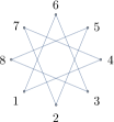
(a)

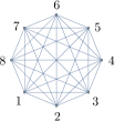
(b)

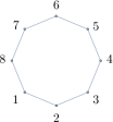
(c)

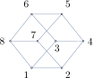
(d)

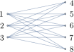
(e)

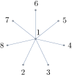
(f)

Figure 1: Families of graphs considered in the main text, with a conventional choice of labelling: (a) circulant graph, (b) complete graph, (c) cycle graph, (d) hypercube graph, (e) complete bipartite graph, (f) star graph.

2.1 Circulant graphs: complete and cycle graphs

A circulant graph $O_{n}$ is a simple graph having the following property: there exists a relabelling of its vertices which is (1) an isomorphism (i.e., any two vertices of the resulting graph are connected by an edge iff they are so connected before the relabelling) and (2) is a cyclic permutation of the vertices (i.e., the relabelling permutes a subset of the vertices in a cyclic fashion, while leaving fixed the remaining ones).

Two special cases of circulant graphs are complete graphs and cycle graphs. A complete graph $K_{n}$ is a graph where each vertex is adjacent to any other vertex. It has $n$ vertices, $n(n-1)/2$ edges and it is regular with degree $n-1$. In the case of a weighted complete graph with all couplings equals, the eigenvalues of the Hamiltonian $H_{K_{n}}$ as in Eq. (2) are:

$$\xi_{j}=\begin{cases}(n-1)(1-\gamma)\qquad\;\text{if $j=0$}\\ (n-1)+\gamma\,\quad\qquad\;\,\text{if $j\neq 0$}\end{cases}\;.$$ (3)

The corresponding eigenvectors are

$$|\xi_{j}\rangle=\frac{1}{\sqrt{n}}\sum_{k=1}^{n}e^{\frac{2\pi ij(k-1)}{n}}\,|k\rangle\;,$$ (4)

where $|k\rangle$ is the position vector corresponding to the $k^{\text{th}}$ vertex.

A cycle graph $C_{n}$ is a chain of $n$ vertices (and as many edges). It is circulant and regular with degree $2$. By specializing to this case Eqs. (53) and (54), found in A, the eigenvalues of $C_{n}$ are found to be

$$\xi_{j}=2-2\gamma\cos\left(\frac{2\pi j}{n}\right)\;,$$ (5)

while the eigenvectors are the same as in Eq. (4).

2.2 Hypercube graphs

A hypercube graph $Y_{d}$ is a regular graph formed from the vertices and edges of the $d$-dimensional hypercube. It has $n=2^{d}$ vertices and $d\cdot 2^{d-1}$ edges; besides, each vertex has the same degree $d$. It can also be thought of as the $d$-fold Cartesian product of the complete graph $K_{2}$. The eigenvalues of the Hamiltonian $H_{Y_{d}}$ for a hypercube graph in dimension $d$ evaluate to

$$\xi_{j}=d-\gamma(d-2j)\;,$$ (6)

while the eigenvectors are computed recursively in the position eigenbasis as the columns of the Hadamard matrices $B_{d}$, $d\in\mathbb{N}$, defined as follows:

$$B_{1}=\frac{1}{\sqrt{2}}\begin{pmatrix}1&1\\ 1&-1\end{pmatrix}\;,\qquad\quad B_{d}=\frac{1}{\sqrt{2}}\begin{pmatrix}B_{d-1}&B_{d-1}\\ B_{d-1}&-B_{d-1}\end{pmatrix}\;.$$ (7)

2.3 Complete bipartite graphs

A complete bipartite graph $K_{p,q}$ is such that its vertex set $V$ can be split into two subsets, with the following property: all vertex of the first set are adjacent to every other vertex of the second, but no two vertices in either sets are adjacent among themselves. It has $n=p+q$ vertices, with $\{1,\dots,p\}$ and $\{p+1,\dots,p+q\}$ denoting the two partitions. A special case of a complete bipartite graph is the star graph $S_{n}=K_{1,n-1}$, corresponding to setting $p=1$ and $q=n-1$. The degenerate spectrum of $H_{K_{p,q}}$ is comprised of the eigenvalues $\{\xi_{1},\xi_{2},\xi_{+},\xi_{-}\}$, where

$$\xi_{1}=q\;,\qquad\xi_{2}=p\;,\qquad\xi_{\pm}=\frac{(p+q)\pm\sqrt{\Delta_{p,q}}}{2}\;,$$ (8)

and we defined $\Delta_{p,q}\mathrel{\hbox to0.0pt{\raisebox{1.29167pt}{$\cdot$}\hss}\raisebox{-1.29167pt}{$\cdot$}}=(p-q)^{2}+4qp\,\gamma^{2}$. The corresponding eigenstates, written in the position eigenbasis, are

$$|\xi_{1}^{(\kappa)}\rangle=(\boldsymbol{a}^{(\kappa)},\,\boldsymbol{0}_{q})^{t}\;,\qquad|\xi_{2}^{(\kappa^{\prime})}\rangle=(\boldsymbol{0}_{p},\,\boldsymbol{b}^{(\kappa^{\prime})})^{t}\;,\qquad|\xi_{\pm}\rangle=\eta_{\pm}\left(\frac{p-\xi_{\pm}}{\gamma p}\,\boldsymbol{1}_{p},\,\boldsymbol{1}_{q}\right)^{t}\;,$$ (9)

where $\eta_{\pm}\mathrel{\hbox to0.0pt{\raisebox{1.29167pt}{$\cdot$}\hss}\raisebox{-1.29167pt}{$\cdot$}}=1/\sqrt{q\left[1+(p-\xi_{\pm})/(q-\xi_{\pm})\right]}$, $\boldsymbol{0}_{q}$ is a $q$-vector made up of all zeros, $\boldsymbol{1}_{q}$ is a $q$-vector made up of all ones, and $\kappa,\,\kappa^{\prime}$ are two degeneracy indexes (see A for more details).

3 Quantum estimation theory

The typical setting in quantum parameter estimation theory is given by a parametric family of quantum states $\{\rho_{\gamma}\}$, smoothly depending on a real parameter $\gamma$. It is assumed that there exists a true value $\gamma^{*}$ such that $\rho_{\gamma^{*}}$ describes the state of the system available to the experimentalist. The main task is to infer the true value from the outcomes of repeated measurements on the system. In fact, if there is no Hermitian operator whose eigenvalues correspond to the possible values of $\gamma$, the parameter cannot be measured directly, and the only possibility is to rely on indirect measurements in order to infer it. More precisely, by preparing $N$ identical copies of the system and repeating $N$ times a measurement $\mathcal{M}$ with sample space $\mathcal{X}$, one obtains a sample $\Omega=\{x_{1},x_{2}\dots,x_{N}\}\in\mathcal{X}^{\times N}$, which is then processed via a local quantum estimator. An estimator is a function $\hat{\gamma}:\Omega\rightarrow\mathbb{R}$ that maps the sample $\Omega$ into an estimate of the parameter. In any quantum estimation procedure, the aim is to optimize over the choice of the measurement in order to maximize the information about the parameter, i.e. to minimize the mean square error of the estimator $\hat{\gamma}$. Because of the inherent stochasticity of quantum measurements, there are strict limitations on the achievable precision. Indeed, the variance of any unbiased estimator is bounded by the Cramér-Rao bound (CRB) as follows:

$$\text{Var}(\hat{\gamma})\geq\frac{1}{N\cdot\mathcal{F}(\mathcal{M},\gamma)}\;,$$ (10)

where $\mathcal{F}(\mathcal{M},\gamma)$ is the Fisher information (FI) associated with the measurement $\mathcal{M}$, i.e.,

$$\mathcal{F}(\mathcal{M},\gamma)=\sum_{x\in\mathcal{X}}p(x|\gamma)\left[\partial_{\gamma}\log p(x|\gamma)\right]^{2}\;,$$ (11)

with $p(x|\gamma)=\tr(\rho_{\gamma}\Pi_{x})$ the conditional probability of obtaining the result $x$ for a measurement $\mathcal{M}$ having positive-operator valued (POVM) elements $\{\Pi_{x}\}_{x\in\mathcal{X}}$, assuming that the value of the parameter is $\gamma$. Minimizing the variance of unbiased estimators is equivalent to maximizing their FI. Therefore, one defines the quantum Fisher Information (QFI) as

$$\mathcal{Q}(\gamma)=\underset{\mathcal{M}}{\max}\;\mathcal{F}(\mathcal{M},\gamma)\;,$$ (12)

which leads to the quantum Cramér-Rao bound (QCRB) [26, 27, 28, 29, 30],

$$\text{Var}(\hat{\gamma})\geq\frac{1}{N\cdot\mathcal{Q}(\gamma)}.$$ (13)

The QCRB establishes the ultimate limit to precision that is imposed by the quantum mechanical nature of the problem. It can always be saturated, at least in the asymptotic regime $N\to\infty$, by employing an asymptotically efficient estimator and implementing the optimal Braunstein-Caves measurement $\mathcal{M}_{\text{opt}}$ [31, 32, 33], defined as:

$$\mathcal{M}_{\text{opt}}\mathrel{\hbox to0.0pt{\raisebox{1.29167pt}{$\cdot$}\hss}\raisebox{-1.29167pt}{$\cdot$}}=\underset{\mathcal{M}}{\text{arg max}}\;\mathcal{F}(\mathcal{M},\gamma)\;.$$ (14)

Remarkably, for pure states $|\psi_{\gamma}\rangle$, a closed-form expression for the QFI is available [25],

$$\mathcal{Q}(\gamma)=4\big{[}\langle\partial_{\gamma}\psi_{\gamma}|\partial_{\gamma}\psi_{\gamma}\rangle+\big{(}\langle\partial_{\gamma}\psi_{\gamma}|\psi_{\gamma}\rangle\big{)}^{2}\big{]}\;,$$ (15)

where $|\partial_{\gamma}\psi_{\gamma}\rangle$ denotes the derivative of the statistical model $|\psi_{\gamma}\rangle$ with respect to the parameter $\gamma$.

In our specific case, the statistical model coincides with the state of the walker at time $t$. As a result, the corresponding QFI still depends on the initial preparation, i.e. on the coefficients $\alpha_{j}$. Therefore, the final step is to maximize the QFI over the choice of such coefficients. In this regard, a useful inequality, to which we will often resort in the following, is Popoviciu’s inequality [35]. Given a bounded probability distribution describing a classical random variable $\mathbb{Y}$, whose minimum and maximum values are denoted by $y$ and $Y$ respectively, Popoviciu’s inequality states that the variance $\text{Var}(\mathbb{Y})$ is bounded as follows,

$$\text{Var}(\mathbb{Y})\leq\frac{1}{4}(Y-y)^{2}\;.$$ (16)

Equality holds whenever half of the probability distribution is peaked at each of the two values.

4 Maximum extractable information vs. performance of selected measurements

Given a quantum walk on a graph $G$ with Hamiltonian $H_{G}$ as in Eq. (2), the problem we are going to consider is to quantify how precisely the tunnelling amplitude $\gamma$ can be estimated via measurements on the walker. In particular, in this section we compute the maximum amount of information on $\gamma$ that can be extracted via any quantum measurement, i.e. the quantum Fisher information $\mathcal{Q}(\gamma)$. Because the QCRB is tight, there always exists a quantum measurement whose FI equals the QFI. However, the optimal measurement may be quite exotic, or even depend on the true value of the parameter, so that it is not necessarily available to the experimentalist. For this reason, we also analyze the performances of a few specific measurements and compare them with the QFI limit. We focus in particular on position measurements. By definition, a position measurement leads to a projection onto the walker’s position basis, i.e. the position operator is $\hat{x}=\sum_{i=1}^{n}j\,|j\rangle\langle j|$. It is also useful to introduce incomplete position measurements. They correspond to coarse-grainings of a position measurement. Explicitly, an incomplete position measurement of size $m$ is represented by a POVM made up of $m$ rank-1 projectors onto $m$ given position eigenstates, plus the projector onto the orthogonal complement of the subspace spanned by them. Incomplete measurements model a situation where one has experimental access only to a subset of the graph’s nodes.

In the following, we first focus on the QFI, studying in particular how it scales with the number of vertices $n$ and the interrogation time $t$, and maximizing it over the initial preparation of the probe. Then, we analyze the performance of position measurements for different graph families, assuming that the initial preparation coincides with the optimal one maximizing the QFI.

4.1 Circulant graphs: complete and cycle graphs

4.1.1 Complete graphs

Let us consider the generic complete graph $K_{n}$. The initial preparation is taken to be $|\psi_{0}\rangle=\sum_{j=0}^{n-1}\alpha_{j}|\xi_{j}\rangle$, where $|\xi_{0}\rangle$ is the ground state and the other energy eigenstates span a degenerate subspace (the corresponding eigenvalues are given in Eq. (3)). The QFI can be easily evaluated via Eq. (15), leading to:

$$\mathcal{Q}_{K_{n}}(\gamma)=4n^{2}t^{2}\,|\alpha_{0}|^{2}(1-|\alpha_{0}|^{2})\;.$$ (17)

Maximizing over the initial preparation, one has that

$$\underset{|\psi_{0}\rangle}{\text{max}}\;\mathcal{Q}_{K_{n}}(\gamma)=n^{2}t^{2},$$ (18)

which is obtained when $|\psi_{0}\rangle$ is equally distributed between the ground state $|\xi_{0}\rangle$ and the excited energy subspace. Notice that the maximum QFI scales quadratically with both the number of vertices $n$ and the interrogation time $t$.

We now want to investigate whether a realistic measurement on the walker allows us to attain the QFI limit of Eq. (18). We thus assume that the state of the walker at time $t=0$ is $\sum_{j=0}^{n}\alpha_{j}|\xi_{j}\rangle$ with $\alpha_{0}=\alpha_{1}=1/\sqrt{2}$ and all other $\alpha_{j}$ set to zero. After a time $t$, an incomplete position measurement of size $m$ is performed. By definition, its POVM consists of the projectors $|j\rangle\langle j|$, for $j\in\{1,\dots,m\}$, plus the projector onto their orthogonal complement $\mathbb{I}_{n}-\sum_{j=0}^{m}|j\rangle\langle j|$. The corresponding FI is denoted by $\mathcal{F}_{K_{n}}^{(m)}(\gamma)$. The efficiency is defined as the ratio of the FI to the QFI, i.e.

$$\eta^{(m)}\mathrel{\hbox to0.0pt{\raisebox{1.29167pt}{$\cdot$}\hss}\raisebox{-1.29167pt}{$\cdot$}}=\frac{\mathcal{F}_{K_{n}}^{(m)}(\gamma)}{\mathcal{Q}_{K_{n}}(\gamma)}\,.$$ (19)

From Eq. (11), the Fisher information $\mathcal{F}_{K_{n}}^{(m)}(\gamma)$ can be written as

$$\mathcal{F}_{K_{n}}^{(m)}(\gamma)=\sum_{j=1}^{m}\frac{(\partial_{\gamma}p_{j})^{2}}{p_{j}}+\frac{(\partial_{\gamma}\bar{p})^{2}}{\bar{p}}\;,$$ (20)

where $p_{j}$ is the probability of detecting the walker at node $j$, i.e.

$$p_{j}=|\langle j|\psi_{t}\rangle|^{2}=\frac{2}{n}\,\cos^{2}\left[\frac{\gamma nt}{2}-\frac{\pi(j-1)}{n}\right]\;,$$ (21)

and $\bar{p}\mathrel{\hbox to0.0pt{\raisebox{1.29167pt}{$\cdot$}\hss}\raisebox{-1.29167pt}{$\cdot$}}=1-\sum_{j=1}^{m}p_{j}$ is the probability that the walker is located outside the subset of the graph’s nodes under control by the experimentalist. It is possible to rewrite $\bar{p}$ as follows,

$$\bar{p}=\frac{n-m}{n}-\frac{1}{n}\cos\left[\gamma nt-\frac{(m-1)\pi}{n}\right]\,\frac{\sin\left(\frac{\pi m}{n}\right)}{\sin\left(\frac{\pi}{n}\right)}\;.$$ (22)

The proof requires first to transform $\cos^{2}(x/2)=(1+\cos x)/2$ and then to simplify the sum over the cosine terms via the geometric series identity

$$\sum_{j=0}^{m-1}e^{i\left(x-\frac{2\pi j}{n}\right)}=e^{ix}\left(\frac{1-e^{-\frac{2\pi im}{n}}}{1-e^{-\frac{2\pi i}{n}}}\right)\;.$$ (23)

The final result for $\mathcal{F}_{K_{n}}^{(m)}(\gamma)$ is

$$\mathcal{F}_{K_{n}}^{(m)}(\gamma)=nt^{2}\left(\!m-\cos\!\left[\gamma nt-\scriptstyle\frac{(m-1)\pi}{n}\right]s_{n,m}+\frac{\sin^{2}\!\left[\gamma nt-\scriptstyle\frac{(m-1)\pi}{n}\right]s_{n,m}^{2}}{(n\!-\!m)\!-\!\cos\!\left[\gamma nt-\scriptstyle\frac{(m-1)\pi}{n}\right]s_{n,m}}\!\right)\;,$$ (24)

where $s_{n,m}\mathrel{\hbox to0.0pt{\raisebox{1.29167pt}{$\cdot$}\hss}\raisebox{-1.29167pt}{$\cdot$}}=\frac{\sin\left(\frac{\pi m}{n}\right)}{\sin\left(\frac{\pi}{n}\right)}$. For instance, if $m=1$:

$$\mathcal{F}_{K_{n}}^{(1)}(\gamma)=\frac{2\sin^{2}\left(\frac{\gamma nt}{2}\right)}{n-2\cos^{2}\left(\frac{\gamma nt}{2}\right)}n^{2}t^{2}\;.$$ (25)

The corresponding efficiency, optimized over the interrogation time $t$, is $\text{max}_{\,t}\;\eta^{(1)}=\frac{2}{n}$. That is, a local measurement can at most extract a fraction $2/n$ of the maximum available information. Vice versa, for a complete position measurement, i.e. $m=n$, one finds from Eq. (24) that $\mathcal{F}^{(n)}_{K_{n}}(\gamma)=n^{2}t^{2}$, which is also equal to the QFI: a complete position measurement is optimal. For a generic incomplete measurement with $1<m<n$, one finds:

$$\underset{t}{\text{max}}\;\eta^{(m)}=\frac{m}{n}+\frac{1}{n}\frac{\sin\left(\frac{\pi m}{n}\right)}{\sin\left(\frac{\pi}{n}\right)}\;.$$ (26)

Using the inequality $\sin(m\pi/n)\leq m\sin(\pi/n)$, the maximum efficiency is at most $2m/n$, i.e. twice the fraction of nodes that can be individually addressed. In particular, the upper bound $2m/n$ is reached when $n\gg m$ and $n\gg 1$.

4.1.2 Cycle graphs

Let us now consider a generic cycle graph $C_{n}$. The QFI evaluates to

$$\mathcal{Q}_{C_{n}}(\gamma)=16t^{2}\,\text{Var}\,\left[\cos\left(\frac{2\pi k\mathbb{X}}{n}\right)\right]\;,$$ (27)

where $\mathbb{X}$ is a random variable, with sample space $j\in\{0,\dots,n-1\}$ and corresponding probabilities $\text{Pr}(j)=|\alpha_{j}|^{2}$. Making use of Popoviciu’s inequality, see Eq. (16), one can maximize the QFI over the initial preparation, which gives:

$$\underset{|\psi_{0}\rangle}{\text{max}}\;\mathcal{Q}_{C_{n}}(\gamma)=\begin{cases}16t^{2}\qquad\qquad&\text{if $n$ even}\\ 4t^{2}\left[1+\cos\left(\frac{\pi}{n}\right)\right]^{2}\quad&\text{if $n$ odd}\end{cases}\,.$$ (28)

The optimal preparation is a balanced superposition of the ground state $|\xi_{0}\rangle$ and highest excited state $|\xi_{n/2}\rangle$, where $\xi_{0}=2(1-\gamma)$, $\xi_{n/2}=2(1+\gamma)$, and the corresponding eigenvectors are defined in Eq. (58). After a time $t$, it gives rise to the state

$$|\psi_{t}\rangle=\frac{1}{\sqrt{2}}e^{-i\xi_{0}t}|\xi_{0}\rangle+\frac{1}{\sqrt{2}}e^{-i\xi_{n/2}t}|\xi_{n/2}\rangle=\frac{1}{\sqrt{2n}}\,e^{-2i(\epsilon-\gamma)t}\,\scriptstyle\begin{pmatrix}\scriptstyle 1+e^{-4i\gamma t}\\ \scriptstyle 1-e^{-4i\gamma t}\\ \scriptstyle\vdots\\ \scriptstyle 1+e^{-4i\gamma t}\\ \scriptstyle 1-e^{-4i\gamma t}\\ \end{pmatrix}\;.$$ (29)

We now analyze the performance of incomplete position measurements taken on the state of Eq. (29). The probability $p_{j}$ of measuring the walker at node $j$ is

$$p_{j}=\frac{1}{n}\,[1+(-1)^{j+1}\cos(4\gamma t)]=\begin{cases}\frac{2}{n}\cos^{2}(2\gamma t)\mathrel{\hbox to0.0pt{\raisebox{1.29167pt}{$\cdot$}\hss}\raisebox{-1.29167pt}{$\cdot$}}=p_{O}\qquad\text{if $j$ is odd}\\[5.0pt] \frac{2}{n}\sin^{2}(2\gamma t)\mathrel{\hbox to0.0pt{\raisebox{1.29167pt}{$\cdot$}\hss}\raisebox{-1.29167pt}{$\cdot$}}=p_{E}\qquad\,\text{if $j$ is even}\end{cases}\;.$$ (30)

Let us assume that the experimentalist has access to a subset of the graph’s nodes, of which $n_{O}$ have an odd label and $n_{E}$ an even label. In the following, we take the total number of vertices $n$ to be even, without loss of generality. Introducing the notation $\beta_{O}\mathrel{\hbox to0.0pt{\raisebox{1.29167pt}{$\cdot$}\hss}\raisebox{-1.29167pt}{$\cdot$}}=2n_{O}/n$ and $\beta_{E}\mathrel{\hbox to0.0pt{\raisebox{1.29167pt}{$\cdot$}\hss}\raisebox{-1.29167pt}{$\cdot$}}=2n_{E}/n$ for, respectively, the fractions of odd and even nodes under individual control, the corresponding Fisher information $\mathcal{F}_{C_{n}}^{(\beta_{0},\beta_{E})}(\gamma)$ can be written as

$$\mathcal{F}_{C_{n}}^{(\beta_{0},\beta_{E})}(\gamma)=n_{O}\frac{(\partial_{\gamma}p_{O})^{2}}{p_{O}}+n_{E}\frac{(\partial_{\gamma}p_{E})^{2}}{p_{E}}+\frac{(\partial_{\gamma}\bar{p})^{2}}{\bar{p}}\;,$$ (31)

where $\bar{p}=1-n_{O}p_{O}-n_{E}p_{E}$. After a standard computation, one finds:

$$\mathcal{F}_{C_{n}}^{(\beta_{0},\beta_{E})}(\gamma)=16t^{2}\;\left[\frac{\beta_{O}+\beta_{E}-2\beta_{O}\beta_{E}+(\beta_{E}-\beta_{O})\cos(4\gamma t)}{2-(\beta_{O}+\beta_{E})+(\beta_{E}-\beta_{O})\cos(4\gamma t)}\right]\;.$$ (32)

In spite of appearances, the previous expression is invariant under relabellings of the graph’s nodes. A relabelling may change the parity of each vertex label, exchanging $\beta_{O}$ with $\beta_{E}$, and $p_{O}$ with $p_{E}$. It is now enough to make use of the relation $\cos(4\gamma t)=np_{O}-1=1-np_{E}$ to check the invariance. From Eq. (32), the efficiency of an incomplete measurement, optimized over the interrogation time $t$, has the following simple expression, i.e.,

$$\underset{t}{\text{max}}\;\eta^{(\beta_{O},\,\beta_{E})}=\text{max}(\beta_{0},\,\beta_{E})\;.$$ (33)

It follows in particular that a complete position measurement is always optimal. Incomplete measurements can also be optimal, e.g. a measurement of only the odd or only the even vertices still has unit efficiency (see also Fig. 2).

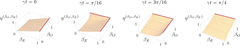
Figure 2: The efficiency $\eta^{(\beta_{O},\beta_{E})}$ of an incomplete measurement, as a function of the fractions of odd nodes $\beta_{O}$ and even nodes $\beta_{E}$ under experimental control, for different values of $\gamma t$. Highlighted by a thick line (red), the optimal region of unit efficiency. For $\gamma t\neq m\pi/4$, $m\in\mathbb{Z}$, the optimal region consists of the two segments $(\beta_{O},1)$ and $(1,\beta_{E})$. For even multiples of $\pi/4$, only the first segment is present, while for odd multiples only the second.

4.2 Hypercube graphs

An hypercube graph $Y_{d}$ has eigenvalues $\xi_{j}$, where $j\in\{0,\dots,d\}$, see Eq. (6). Each eigenvalue $\xi_{j}$ has multiplicity $[d,j]\mathrel{\hbox to0.0pt{\raisebox{1.29167pt}{$\cdot$}\hss}\raisebox{-1.29167pt}{$\cdot$}}=d!/j!(d-j)!$. The corresponding eigenstates $|\xi_{j}^{(\kappa_{j})}\rangle$, with $\kappa_{j}\in\{1,\dots,[d,j]\}$, are constructed recursively for any $d$ by means of Eq. (7). The most general initial preparation is

$$|\psi_{0}\rangle=\sum_{j=0}^{d}\sum_{\kappa_{j}=1}^{[d,j]}\,\alpha_{j}^{(\kappa_{j})}|\xi_{j}^{(\kappa_{j})}\rangle\;,\qquad\text{with}\quad\sum_{j=0}^{d}\sum_{\kappa_{j}=1}^{[d,j]}|\alpha_{j}^{(\kappa_{j})}|^{2}=1\;.$$ (34)

For future convenience, let us denote by $p_{\xi_{j}}\mathrel{\hbox to0.0pt{\raisebox{1.29167pt}{$\cdot$}\hss}\raisebox{-1.29167pt}{$\cdot$}}=\sum_{\kappa_{j}=1}^{[d,j]}|\alpha_{j}^{(\kappa_{j})}|^{2}$ the total probability that an energy measurement returns the outcome $\xi_{j}$. It can be checked that the QFI at time $t$ and for a generic initial state can be written as:

$$\mathcal{Q}_{Y_{d}}(\gamma)=4t^{2}\,\text{Var}(d-2\mathbb{X})\;,$$ (35)

where $\mathbb{X}$ is a random variable such that $\text{Pr}(j)=p_{\xi_{j}}$, for $j\in\{0,\dots,d\}$. Since the maximum value of $d-2\mathbb{X}$ is equal to $d$ (when $\mathbb{X}=0$) and the minimum value is $-d$ (when $\mathbb{X}=d$), one has that $\mathcal{F}_{Q}(\gamma)\leq 4t^{2}d^{2}$ by Popoviciu’s inequality. The optimal QFI thus evaluates to

$$\underset{|\psi_{0}\rangle}{\text{max}}\;\mathcal{Q}_{Y_{d}}(\gamma)=4t^{2}d^{2},$$ (36)

which scales quadratically with the dimension $d$ and the interrogation time $t$. The optimal preparation is a balanced superposition of the ground state $|\xi_{0}\rangle$ and the maximally excited state $|\xi_{d}\rangle$ (see Eq. (61)).

Let us now consider the performance of incomplete position measurements. After a time $t$, an incomplete position measurement is performed on the state $|\psi_{t}\rangle=(e^{-i\xi_{0}t}|\xi_{0}\rangle+e^{-i\xi_{d}t}|\xi_{d}\rangle)/\sqrt{2}$, where $\xi_{0}=d(1-\gamma)$, $\xi_{d}=d(1+\gamma)$. We adopt the following notation: $\mathcal{F}_{Y_{d}}^{(\delta)}(\gamma)$ denotes the Fisher information for an incomplete measurement having as POVM the $2^{\delta}$ rank-1 projectors over the nodes making up a $\delta$-dimensional face of the hypercube, plus the projector onto their orthogonal complement. It can be computed as

$$F_{Y_{d}}^{(\delta)}(\gamma)=2^{\delta-1}\,\frac{(\partial_{\gamma}p_{+})^{2}}{p_{+}}+2^{\delta-1}\frac{(\partial_{\gamma}p_{-})^{2}}{p_{-}}\;,$$ (37)

where

$$p_{+}\mathrel{\hbox to0.0pt{\raisebox{1.29167pt}{$\cdot$}\hss}\raisebox{-1.29167pt}{$\cdot$}}=\frac{1}{2^{d-1}}\,\cos^{2}(d\gamma t)\;,\qquad\quad p_{-}\mathrel{\hbox to0.0pt{\raisebox{1.29167pt}{$\cdot$}\hss}\raisebox{-1.29167pt}{$\cdot$}}=\frac{1}{2^{d-1}}\,\sin^{2}(d\gamma t)\;.$$ (38)

Notice that the probability of finding the walker in any of the accessible nodes is $2^{\delta-1}p_{+}+2^{\delta-1}p_{-}=1/2^{d-\delta}$, which is, in particular, independent of $\gamma$. Thus, no term analogous to the last one on the right-hand-side of Eq. (20) appears in Eq. (37). The FI evaluates to

$$\mathcal{F}_{Y_{d}}^{(\delta)}(\gamma)=2^{\delta-d+2}d^{2}t^{2}\;.$$ (39)

Its efficiency is $\eta^{(\delta)}=1/2^{d-\delta}$, i.e. the ratio between the number of nodes under individual control and the total number of nodes. It follows that, in particular, a complete measurement (when $\delta=d$) is optimal.

4.3 Complete bipartite graphs

The generic complete bipartite graph $K_{p,q}$ has $n=p+q$ eigenvectors, of which only two, $|\xi_{\pm}\rangle$ given in Eq. (8), depend on the parameter $\gamma$. All other eigenvectors, as well as their eigenvalues, are independent of $\gamma$; thus, no estimation strategy can fruitfully make use of them. As a consequence, the initial preparation is taken to be a superposition of $|\xi_{\pm}\rangle$ only, e.g. $|\psi_{0}\rangle=\alpha_{-}|\xi_{-}\rangle+\alpha_{+}|\xi_{+}\rangle$. The corresponding QFI at the generic time $t$ evaluates to

$$\mathcal{Q}_{K_{p,q}}(\gamma)=\frac{4\left(f_{p,q}-4g_{p,q}^{2}\right)}{\Delta_{p,q}^{2}}\;,$$ (40)

where

$$f_{p,q}=pq[16p^{2}q^{2}\gamma^{4}t^{2}+(p-q)^{2}(1+4pq\gamma^{2}t^{2})]\;,$$ (41)

$$g_{p,q}=(|\alpha_{-}|^{2}-|\alpha_{+}|^{2})\,pq\gamma t\sqrt{\Delta_{p,q}}+\Im\left(e^{it\sqrt{\Delta_{p,q}}}\bar{\alpha}_{+}\alpha_{-}\right)(p-q)\sqrt{pq}\;.$$ (42)

The optimal initial preparation is such that $g_{p,q}$ vanishes, which is obtained when $|\alpha_{-}|=|\alpha_{+}|$, with a relative phase $\phi_{\text{opt}}=\text{arg}(\alpha_{+}/\alpha_{-})=t\sqrt{\Delta_{p,q}}$. The maximum QFI is therefore equal to

$$\underset{|\psi_{0}\rangle}{\text{max}}\;\mathcal{Q}_{K_{p,q}}(\gamma)=4f_{p,q}/\Delta_{p,q}^{2}.$$ (43)

For fixed number of vertices $n$, one may further optimize over the cardinality of each bipartition $p$ and $q$. The maximum is reached for $p=\lfloor n/2\rfloor$, which leads to a corresponding scaling $\sim n^{2}t^{2}$, quadratic both in the number of vertices and the interrogation time.

We now study in some detail the special case of a star graph $S_{n}$. The maximum QFI is obtained via the substitutions $p=1$ and $q=n-1$,

$$\underset{|\psi_{0}\rangle}{\text{max}}\;\mathcal{Q}_{S_{n}}(\gamma)=\frac{4(n-1)[16(n-1)^{2}\,\gamma^{4}t^{2}+(n-2)^{2}[1+4(n-1)\gamma^{2}t^{2}]]}{[(n-2)^{2}+4(n-1)\gamma^{2}]^{2}}\;.$$ (44)

It depends on $n$, but does not grow indefinitely with the size of the graph. When $n\to\infty$, it saturates instead to a constant value. Therefore, an optimal number of nodes $n_{\text{opt}}$ may exist. We solve for $n_{\text{opt}}$ in the two opposite regimes of small and long times. For small times $\gamma t\ll 1$,

$$\underset{|\psi_{0}\rangle}{\text{max}}\;\mathcal{Q}_{S_{n}}(\gamma)\sim\frac{4(n-1)(n-2)^{2}}{[(n-2)^{2}+4(n-1)\gamma^{2}]^{2}}\;,$$ (45)

which is maximized by

$$n_{\text{opt}}\sim 2[1+\gamma^{2}+\gamma\sqrt{1+\gamma}].$$ (46)

For large times $\gamma t\gg 1$,

$$\underset{|\psi_{0}\rangle}{\text{max}}\;\mathcal{Q}_{S_{n}}(\gamma)\sim\frac{16\gamma^{2}t^{2}(n-1)[4(n-1)^{2}\gamma^{2}+(n-2)^{2}(n-1)]}{[(n-2)^{2}+4(n-1)\gamma^{2}]^{2}}\;.$$ (47)

If $1/\gamma^{2}\leq 2$, then there is no optimal value of $n$ (the optimal value is $n=\infty$). Instead, if $1/\gamma^{2}>2$, the optimal value of $n$ is

$$n_{\text{opt}}\sim\frac{2(1/\gamma^{2}-1)}{(1/\gamma^{2}-2)}\;.$$ (48)

Adding new vertices above $n_{\text{opt}}$ will lower the maximum achievable precision.

From our previous discussion, the optimal initial preparation is a balanced superposition of the two energy eigenstates $|\xi_{\pm}\rangle$ that can be read off from Eq. (67) after setting $p=1$ and $q=n-1$, with a relative phase $\phi_{\text{opt}}=t\sqrt{\Delta_{1,n-1}}$. Since the optimal phase $\phi_{\text{opt}}$ depends on $\gamma$, an adaptive procedure is required in order to extract the maximum QFI. For the moment, we assume that the walker is prepared in the state $|\psi_{0}\rangle=(|\xi_{-}\rangle+e^{i\phi}|\xi_{+}\rangle)/\sqrt{2}$, where $\phi\in[0,2\pi]$ is arbitrary. Let us suppose that at time $t$ an incomplete position measurement is performed. First, we consider the case of an incomplete measurement monitoring only the central node, with associated POVM made up of the two projectors $|1\rangle\langle 1|$ and $\mathbb{I}_{n}-|1\rangle\langle 1|$. One finds that its Fisher information coincides with the FI for a complete position measurement, denoted by $\mathcal{F}_{S_{n}}^{(\phi)}(\gamma)$ (the superscript makes manifest the dependence on the arbitrary phase $\phi$ of the initial state). The implication is that distinguishing outcomes corresponding to the walker being in one peripheral node or the other is useless for estimation purposes: one may as well monitor only the central node. The efficiency $\eta^{(\phi)}$ of a position measurement (either a complete measurement or an incomplete one, but including the central node) is

$$\eta^{(\phi)}=\;\frac{(n-1)[(n-2)^{2}\cos(\phi_{\text{opt}}-\phi)-4(n-1)\sqrt{\Delta_{1,n-1}}\,\gamma^{2}t\sin(\phi_{\text{opt}}-\phi)]^{2}}{f_{1,n-1}\left[4(n-1)\gamma^{2}\sin^{2}(\phi_{\text{opt}}-\phi)+(n-2)^{2}\right]}\;.$$ (49)

Except for a few special cases (when $n=2$, or $t=0$ and $\phi=\phi_{\text{opt}}$), a position measurement is always suboptimal. For short interrogation times, expanding for $\gamma t\ll 1$ and $\phi=\phi_{\text{opt}}$, one obtains

$$\eta^{(\phi_{\text{opt}})}=1-\frac{4(n-1)\Delta_{1,n-1}}{(n-2)^{4}}\gamma^{2}t^{2}+o(\gamma^{2}t^{2})\;,\qquad\qquad(\gamma t\to 0)\;.$$ (50)

For large number of vertices $n\to\infty$ and $\phi=\phi_{\text{opt}}$, one has instead

$$\eta^{(\phi_{\text{opt}})}=\frac{1}{4\gamma^{2}t^{2}n}+o(1/n)\;,\qquad\qquad(n\to\infty),$$ (51)

i.e. the efficiency decreases linearly with the number of vertices. The reader is also referred to Fig. 3 for more details about the different possible regimes.

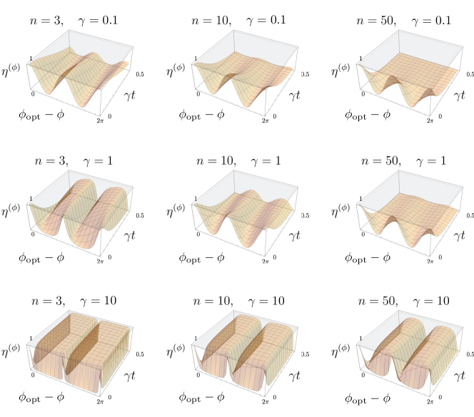
Figure 3: The efficiency $\eta^{(\phi)}$ of a complete measurement, as a function of the phase difference $\phi_{{\text{opt}}}-\phi$ and of the dimensionless time scale $\gamma t$ (for different values of $n$ and $\gamma$). In general, the efficiency is closer to one for higher values of $\gamma$ and for smaller values of $\gamma t$ and of $n$. Only for $t=0$, there always exist a choice of $\phi$ which allows to reach unit efficiency; otherwise, a complete measurement is suboptimal.

	scaling of QFI with $n$	optimal preparation	optimal measurement	$\eta$ of incomplete position measurement
$K_{n}$	$\sim n^{2}$	any balanced superposition of ground state and any other excited state	position	$\beta+1/n\cdot\sin(\pi\beta)/\sin(\pi/n)$
$C_{n}$	$\begin{cases}$independent of $n&\mbox{if $n$ even }\\ \sim\left[1+\cos\left(\frac{\pi}{n}\right)\right]^{2}&\mbox{if $n$ odd}\end{cases}$	any balanced superposition of ground state and highest excited state	position	$\text{max}(\beta_{O},\,\beta_{E})$
$Y_{d}$	$\sim(\log n)^{2}$	any balanced superposition of ground state and highest excited state	position	$\beta$
$S_{n}$	$\exists\;n_{\text{opt}}$	balanced superposition of $|\xi_{\pm}\rangle$ with relative phase $\phi_{\text{opt}}$	exotic	independent of $\beta$

Table 1: For each family of graphs considered in the main text, we report the scaling of the QFI with the total number of nodes $n$, the optimal measurement saturating the quantum Cramér-Rao bound, the optimal initial preparation and the efficiency $\eta$ of an incomplete position measurement. Notice that $\beta$ (resp., $\beta_{O}$, $\beta_{E}$) denotes the fraction of the graphs’s nodes (resp., nodes with even labels, odd labels) under individual control by the experimentalist.

5 Conclusions

In this paper, we have studied the problem of estimating the tunnelling amplitude $\gamma$ for a quantum walker evolving continuously in time on a graph $G$, where $G$ is an element of a few relevant families of graphs. Our first result is that the topology of the graph may have dramatic effects on the maximum extractable information. For instance, the quantum Fisher information exhibits different scaling laws with the total number of vertices (see Table 1). For each family considered, we have maximized the quantum Fisher information over the initial preparation, determining the optimal initial state of the walker, as well as the optimal measurement.

We have then discussed in details the performance of position measurements. Complete position measurements, which may implemented when one has experimental access to the full set of graph’s node, perform quite well: they are often optimal, the only exception being (among the cases taken into consideration) that of complete bipartite graphs, e.g. star graphs. Incomplete, e.g. nearly-local, position measurements still allow to extract a non-vanishing amount of information. Their efficiency (i.e. the ratio of the FI to QFI) is closely related to the fraction $\beta$ of the graph’s nodes that are under control by the experimentalist. The exception is again the case of star graphs, since monitoring only the central node yields the same information as monitoring each node separately.

Our results uncover fundamental properties of quantum walks related to their topologies, and pave the way to optimal design of quantum walks implementation, e.g. with superconducting circuits.

Appendix A Spectral properties of selected graphs

Circulant graphs: complete and cycle graphs

The adjacency matrix of a circulant graph $O_{n}$ is a circulant matrix, i.e. each row is obtained by shifting the preceding one to the right. Denoting by $d$ the degree of each vertex, we consider the following quantum walk Hamiltonian on $O_{n}$:

$$H_{O_{n}}=\begin{pmatrix}d&-\gamma_{1}&-\gamma_{2}&\dots&-\gamma_{n-1}\\ -\gamma_{n-1}&d&-\gamma_{1}&\dots&-\gamma_{n-2}\\ -\gamma_{n-2}&-\gamma_{n-1}&d&\dots&-\gamma_{n-3}\\ \vdots&\vdots&\vdots&\ddots&\vdots\\ -\gamma_{1}&-\gamma_{2}&-\gamma_{3}&\dots&d\end{pmatrix}\;.$$ (52)

We impose the symmetry constraint $\gamma_{j}=\gamma_{n-j}$, so that $H_{O_{n}}$ is itself a circulant matrix. Notice that there are a total of $\lfloor n/2\rfloor$ independent couplings. In particular, if all weights are set equal to the same value, Eq. (52) reduces to the case of a complete graph $K_{n}$; if instead the only non-zero weights are $\gamma_{1}=\gamma_{n-1}$ one has a cycle graph $C_{n}$.

From the general theory of circulant matrices [34], the eigenvalues of $H_{O_{n}}$ are found to be

$$\xi_{j}=d-\sum_{k=1}^{n-1}\gamma_{k}\,e^{\frac{2\pi ijk}{n}}\;,\qquad\qquad j\in\{0,\dots,n-1\}\;.$$ (53)

Using the fact that $\gamma_{j}=\gamma_{n-j}$, one may rewrite the previous equation as

$$\xi_{j}=\begin{cases}d-2\gamma_{1}\cos\left(\frac{2\pi j}{n}\right)-\dots-2\gamma_{(n-2)/2}\cos\left(\frac{(n-2)\pi j}{n}\right)-\gamma_{n/2}\cos\left(\pi j\right)\quad\,\text{($n$ even)}\\[10.0pt] d-2\gamma_{1}\cos\left(\frac{2\pi j}{n}\right)-\dots-2\gamma_{(n-1)/2}\cos\left(\frac{(n-1)\pi j}{n}\right)\quad\qquad\qquad\;\,\qquad\text{($n$ odd)}\end{cases}\;.$$

Notice that the spectrum is doubly degenerate, i.e. $\xi_{j}=\xi_{n-j}$. The eigenvectors are

$$|\xi_{j}\rangle=\frac{1}{\sqrt{n}}\sum_{k=1}^{n}e^{\frac{2\pi ij(k-1)}{n}}\,|k\rangle\;.$$ (54)

Complete graphs

When all couplings are equal among themselves, the Hamiltonian of Eq. (52) reduces to:

$$H_{K_{n}}=\begin{pmatrix}(n-1)&-\gamma&-\gamma&\dots&-\gamma\\ -\gamma&(n-1)&-\gamma&\dots&-\gamma\\ \vdots&\vdots&\vdots&\ddots&\vdots\\ -\gamma&-\gamma&-\gamma&\dots&(n-1)\end{pmatrix}\;.$$ (55)

Making use of Eq. (53) and the identity $\sum_{k=0}^{n-1}\text{exp}(2\pi jk/n)=0$, the eigenvalues of $H_{K_{n}}$ can be written more compactly as

$$\xi_{j}=\begin{cases}(n-1)(1-\gamma)\qquad\text{if $j=0$}\\ (n-1)+\gamma\;\quad\qquad\text{if $j\neq 0$}\end{cases}\;.$$ (56)

The least eigenvalue is $\xi_{0}$, whereas the remaining eigenvalues are all degenerate. The corresponding eigenvectors are the same as in Eq. (54).

Cycle graphs

For cycle graphs, all couplings are zero except for $\gamma_{1}=\gamma_{n-1}$. The Hamiltonian $H_{C_{n}}$ is

$$H_{C_{n}}=\begin{pmatrix}2&-\gamma&0&\dots&-\gamma\\ -\gamma&2&-\gamma&\dots&0\\ 0&-\gamma&2&\dots&0\\ \vdots&\vdots&\vdots&\ddots&\vdots\\ -\gamma&0&0&\dots&2\end{pmatrix}\;.$$ (57)

In the main text, the case of a cycle graph with an even number of vertices is considered. Specializing some of the above formulas, the least eigenvalue of $H_{C_{n}}$ is found to be $\xi_{0}=2(1-\gamma)$, while the largest is $\xi_{n/2}=2(1+\gamma)$, with corresponding eigenvectors

$$|\xi_{0}\rangle=\frac{1}{\sqrt{n}}(1,1\dots,1,1)^{t}\qquad\text{and}\qquad|\xi_{n/2}\rangle=\frac{1}{\sqrt{n}}(1,-1\dots,1,-1)^{t}\;.$$ (58)

Hypercube graphs

For a generic hypercube graph $Y_{d}$, its quantum walk Hamiltonian can be written as $H_{Y_{d}}=d\,\mathbb{I}_{2^{d}}-\gamma A^{(d)}$, where $A^{(d)}$ is the adjacency matrix of $Y_{d}$, which is defined recursively via the following relation:

$$A^{(1)}=\begin{pmatrix}0&1\\ 1&0\\ \end{pmatrix}\;,\qquad\qquad A^{(d)}=\begin{pmatrix}A^{(d-1)}&\mathbb{I}_{2^{d-1}}\\ \mathbb{I}_{2^{d-1}}&A^{(d-1)}\end{pmatrix}\;.$$ (59)

The eigenvectors of $H_{Y_{d}}$ are denoted by $|\xi_{j}^{(\kappa_{j})}\rangle$, where $j\in\{0,\dots,d\}$ and $\kappa_{j}$ is a degeneracy index ranging from 1 to $[d,j]\mathrel{\hbox to0.0pt{\raisebox{1.29167pt}{$\cdot$}\hss}\raisebox{-1.29167pt}{$\cdot$}}=d!/j!(d-j)!$. The corresponding eigenvalues are $\xi_{j}=d-\gamma(d-2j)$. The eigenvectors $|\xi_{j}^{(\kappa_{j})}\rangle$ coincide with the columns of a sequence of matrices $B_{d}$, indexed by the dimension $d$ and defined recursively as follows:

$$B_{1}=\frac{1}{\sqrt{2}}\begin{pmatrix}1&1\\ 1&-1\end{pmatrix}\;,\qquad\qquad B_{d}=\frac{1}{\sqrt{2}}\begin{pmatrix}B_{d-1}&B_{d-1}\\ B_{d-1}&-B_{d-1}\end{pmatrix}\;.$$ (60)

By construction, each $B_{d}$ is a Hadamard matrix. In particular, the ground state $|\xi_{0}\rangle$ and the highest excited state $|\xi_{d}\rangle$ can be written as:

$$|\xi_{0}\rangle=\frac{1}{2^{d/2}}\begin{pmatrix}1\\ 1\end{pmatrix}^{\!\otimes\,d}\;,\qquad\qquad|\xi_{d}\rangle=\frac{1}{2^{d/2}}\begin{pmatrix}1\\ -1\end{pmatrix}^{\!\otimes\,d}\;.$$ (61)

Notice that they are non-degenerate, i.e. $\kappa_{0}=\kappa_{d}=1$, so we omit the degeneracy label.

Complete bipartite graphs

For a complete bipartite graph $K_{p,q}$, the quantum walk Hamiltonian $H_{K_{p,q}}$ takes the following block form:

$$H_{K_{p,q}}=\left(\begin{array}[]{c|c}q\,\mathbb{I}_{p}&-\gamma\mathbb{J}_{p\times q}\\ \hline\cr-\gamma\mathbb{J}_{q\times p}&p\,\mathbb{I}_{q}\end{array}\right)\;,$$ (62)

where $\mathbb{I}_{p}$ is the $p\times p$ identity matrix and $\mathbb{J}_{p\times q}$ is the $p\times q$ matrix made up of all ones. In the position eigenbasis, a natural ansatz for the generic eigenvector $|\xi\rangle$ of $H_{K_{p,q}}$ is in the form $|\xi\rangle=(\boldsymbol{x},\,\boldsymbol{y})^{t}$, where $\boldsymbol{x}$ is a $p$-vector and $\boldsymbol{y}$ a $q$-vector. The eigenvalue equation $H_{K_{p,q}}|\xi\rangle=\xi\cdot|\xi\rangle$ implies the linear system of constraints:

$$\begin{cases}(q-\xi)\boldsymbol{x}=\gamma\mathbb{J}_{p\times q}\,\boldsymbol{y}\\ (p-\xi)\boldsymbol{y}=\gamma\mathbb{J}_{q\times p}\,\boldsymbol{x}\end{cases}\;.$$ (63)

Multiplying by $\mathbb{J}_{q\times p}$ the first of the previous equations and by $\mathbb{J}_{p\times q}$ the second equation, and using the fact that $\mathbb{J}_{q\times p}\,\mathbb{J}_{p\times q}=p\,\mathbb{J}_{q\times q}$, one obtains:

$$\mathbb{J}_{q\times q}\,\boldsymbol{y}=\frac{(q-\xi)(p-\xi)}{\gamma^{2}p}\,\boldsymbol{y}\;,\qquad\mathbb{J}_{p\times p}\,\boldsymbol{x}=\frac{(q-\xi)(p-\xi)}{\gamma^{2}q}\,\boldsymbol{x}\;.$$ (64)

It follows that $\boldsymbol{y}$ is an eigenvector of $\mathbb{J}_{q\times q}$and $\boldsymbol{x}$ is an eigenvector of $\mathbb{J}_{p\times p}$. Let us recall that the spectrum of $\mathbb{J}_{p\times p}$ is made up of the eigenvalue $0$ (with multiplicity $p-1$ and corresponding eigenspace spanned by all $p$-vectors whose components sum to zero) and the eigenvalue $p$ (with multiplicity 1 and corresponding eigenvector $\boldsymbol{1}_{p}$, the $p$-vector made up of ones). Eqs. (64) thus imply that the only possible values for $\xi$ are $\text{spec}(H_{G})=\{\xi_{1},\,\xi_{2},\,\xi_{+},\xi_{-}\}$, where $\xi_{1}\mathrel{\hbox to0.0pt{\raisebox{1.29167pt}{$\cdot$}\hss}\raisebox{-1.29167pt}{$\cdot$}}=q$, $\xi_{2}\mathrel{\hbox to0.0pt{\raisebox{1.29167pt}{$\cdot$}\hss}\raisebox{-1.29167pt}{$\cdot$}}=p$ and $\xi_{\pm}$ are the roots of the equation $(q-\xi_{\pm})(p-\xi_{\pm})=qp\,\gamma^{2}$, i.e.

$$\xi_{\pm}=\frac{(p+q)\pm\sqrt{\Delta_{p,q}}}{2}\;,\qquad\quad\text{with}\qquad\Delta_{p,q}\mathrel{\hbox to0.0pt{\raisebox{1.29167pt}{$\cdot$}\hss}\raisebox{-1.29167pt}{$\cdot$}}=(p-q)^{2}+4qp\,\gamma^{2}\;.$$ (65)

Notice that the lowest eigenvalue is $\xi_{-}$, the highest is $\xi_{+}$, while $\xi_{1}$ and $\xi_{2}$ are always in between.

The corresponding eigenvectors can be found as follows. For the eigenvalue $\xi_{1}$, one finds that $\boldsymbol{y}$ must vanish and that $\boldsymbol{x}\in\text{ker}\,{\mathbb{J}_{p\times p}}$, whereas for $\xi_{2}$, $\boldsymbol{x}$ must vanish and $\boldsymbol{y}\in\text{ker}\,{\mathbb{J}_{q\times q}}$. Introducing two orthonormal basis $\boldsymbol{a}^{(\kappa)}$ and $\boldsymbol{b}^{(\kappa^{\prime})}$, for $\text{ker}\,{\mathbb{J}_{p\times p}}$ and $\text{ker}\,{\mathbb{J}_{q\times q}}$ respectively, one can write:

$$|\xi_{1}^{(\kappa)}\rangle=(\boldsymbol{a}^{(\kappa)},\boldsymbol{0}_{q})^{t}\;,\qquad\qquad|\xi_{2}^{(\kappa^{\prime})}\rangle=(\boldsymbol{0}_{p},\boldsymbol{b}^{(\kappa^{\prime})})^{t}\;,$$ (66)

where $\kappa\in\{1,\dots,p-1\}$ and $\kappa^{\prime}\in\{1,\dots,q-1\}$. For the remaining two eigenvalues $\xi_{\pm}$, after substituting into the eigenvalue equation, one finally finds

$$|\xi_{\pm}\rangle=\eta_{\pm}\begin{pmatrix}\frac{p-\xi_{\pm}}{\gamma p}\,\boldsymbol{1}_{p}\\ \boldsymbol{1}_{q}\end{pmatrix}\;,\qquad\quad\text{with}\qquad\eta_{\pm}\mathrel{\hbox to0.0pt{\raisebox{1.29167pt}{$\cdot$}\hss}\raisebox{-1.29167pt}{$\cdot$}}=\left[q\left(1+\frac{p-\xi_{\pm}}{q-\xi_{\pm}}\right)\right]^{-1/2}\;.$$ (67)

Since Eqs. (66) and (67) already define a set of $p+q$ orthonormal eigenvectors, there are no additional eigenvectors.

References

References

- [1] E. Farhi and S. Gutmann, Quantum computation and decision trees, Phys. Rev. A 58, 915 (1998).
- [2] J. Kempe, Quantum random walks - an introductory overview, Contemp. Phys. 44, 307 (2003).
- [3] S. E. Venegas-Andraca, Quantum walks: a comprehensive review, Quantum Inf. Proc. 11, 1015 (2012).
- [4] A. M. Childs, Universal Computation by Quantum Walk, Phys. Rev. Lett. 102, 180501 (2009).
- [5] A. M. Childs and J. Goldstone, Spatial search by quantum walk, Phys. Rev. A 70, 022314 (2004).
- [6] V. Kendon, A random walk approach to quantum algorithms, Phil. Trans. R. Soc. A 364, 3407 (2006).
- [7] A. Ambainis, Quantum walk algorithm for element distinctness, SIAM J. Comput., 37, 210 (2007).
- [8] E. Farhi, J. Goldstone, and S. Gutmann, A quantum algorithm for the hamiltonian NAND tree, Theory Comput. 4, 169 (2008).
- [9] J. K. Gamble, M. Friesen, D. Zhou, R. Joynt, S. N. Coppersmith, Two-particle quantum walks applied to the graph isomorphism problem, Phys. Rev. A 81, 052313 (2010).
- [10] O. Mülken and A. Blumen, Continuous-time quantum walks: Models for coherent transport on complex networks, Phys. Rep. 502, 37 (2011).
- [11] R. Alvir, S. Dever, B Lovitz, J. Myer, C. Tamon, Y. Xu, H. Zhan, Perfect State Transfer in Laplacian Quantum Walk, J. Algebr. Comb. 43, 801 (2016).
- [12] D. Tamascelli, S. Olivares, S. Rossotti, R. Osellame and M. G. A. Paris,, Quantum state transfer via Bloch oscillations, Sci. Rep. 6, 26054 (2016).
- [13] M. Mohseni, P. Rebentrost, S. Lloyd, A. Aspuru-Guzik, Environment-assisted quantum walks in photosynthetic energy transfer J. Chem. Phys. 129, 174106 (2008).
- [14] S. Hoyer, M. Sarovar, K. B. Whaley, Limits of quantum speedup in photosynthetic light harvesting, New J. Phys. 12, 065041 (2010).
- [15] P. M. Preiss, R. Ma, M. E. Tai, A. Lukin, M. Rispoli, P. Zupancic, Y. Lahini, R. Islam, and M. Greiner, Strongly correlated quantum walks in optical lattices, Science 347, 6227 (2015).
- [16] A. Peruzzo, M. Lobino, J. C. F. Matthews, N. Matsuda, A. Politi, K. Poulios, X. Zhou, Y. Lahini, N. Ismail, K. Wörhoff, Y. Bromberg, Y. Silberberg, M. G. Thompson, and J. L. OBrien, Quantum walks of correlated photons, Science 329, 5998 (2010).
- [17] A. Hines and P. C. E. Stamp, Quantum walks, quantum gates, and quantum computers, Phys. Rev. A 75, 062321(2007).
- [18] D. Burgarth, and K. Maruyama, Indirect Hamiltonian identification through a small gateway., New J. Phys. 11, 103019 (2009).
- [19] M. Hillery, H. Zheng, E. Feldman, D. Reitzner, V. Buzek, Quantum walks as a probe of structural anomalies in graphs, Phys. Rev. A 85, 062325 (2012).
- [20] D. Tamascelli, C. Benedetti, S. Olivares, M. G. A. Paris, Characterization of qubit chains by Feynman probes, Phys. Rev. A 94, 042129 (2016).
- [21] J. Nokkala, S. Maniscalco and J. Piilo , Local probe for connectivity and coupling strength in quantum complex networks, Sci. Rep. 8, 13010 (2018).
- [22] T. Ito, T. Otsuka, S. Amaha, M. R. Delbecq, T. Nakajima, J. Yoneda, K. Takeda, G. Allison, A. Noiri, K. Kawasaki and S. Tarucha, Detection and control of charge states in a quintuple quantum dot, Sci. Rep. 6, 39113 (2016).
- [23] A. A. Melnikov, L. E. Fedichkin, Quantum walks of interacting fermions on a cycle graph, Sci. Rep. 6, 34226 (2016)
- [24] J. P. Zwolak, S. S. Kalantre, X. Wu, S. Ragole, J. M. Taylor, QFlow lite dataset: A machine-learning approach to the charge states in quantum dot experiments, PLOS ONE 13 (10), e0205844 (2018).
- [25] M. G. A. Paris, Quantum estimation for quantum technology, Int. J. Quantum Inf. 7, 125 (2009).
- [26] C. W. Helstrom, Quantum detection and estimation theory, Academic Press (1976).
- [27] A. Fujiwaraa, H. Nagaoka Quantum Fisher metric and estimation for pure state models, Phys. Lett. A, 201, 119 (1995).
- [28] D. Petz, Monotone metrics on matrix spaces, Lin. Alg. Appl. 244, 81 (1996).
- [29] D. C. Brody, L. P. Hughston, Statistical geometry in quantum mechanics, Proc. Roy. Soc. A 454, 2445 (1998).
- [30] J. Liu, H.-N. Xiong, F. Song, X. Wang, Fidelity susceptibility and quantum Fisher information for density operators with arbitrary ranks, Physica A 410, 167 (2014).
- [31] S. L. Braunstein and C. M. Caves, Statistical distance and the geometry of quantum states, Phys. Rev. Lett. 72 3439 (1994).
- [32] S. L. Braunstein, C. M. Caves, and G. J. Milburn, Generalized Uncertainty Relations: Theory, Examples, and Lorentz Invariance, Ann. Phys. 247, 135 (1996).
- [33] H. Nagaoka, An asymptotically efficient estimator for a one-dimensional parametric model of quantum statistical operators, Proc. Int. Symp. on Inform. Theory, 198, 577 (1988).
- [34] R. Aldrovandi, Special matrices of mathematical physics: stochastic, circulant, and Bell matrices, World Scientific (2001).
- [35] T. Popoviciu, Sur les équations algébriques ayant toutes leurs racines réelles, Mathematica 9, 129 (1935).