Discrete Optimal Control of Interconnected Mechanical Systems

Abstract

This article develops variational integrators for a class of underactuated mechanical systems using the theory of discrete mechanics. Further, a discrete optimal control problem is formulated for the considered class of systems and subsequently solved using variational principles again, to obtain necessary conditions that characterise optimal trajectories. The proposed approach is demonstrated on benchmark underactuated systems and accompanied by numerical simulations.

I INTRODUCTION

A particular problem in optimal control of mechanical systems involves transferring a system from its current state to a desired state while minimizing a cost function (like control effort or time). There are two standard methods of approaching this problem. In the first method, the equations of motion are derived using variational principles. Then these differential equations are discretized and applied as algebraic constraints to a nonlinear optimization program to obtain the minimum cost trajectory. The second method involves obtaining optimality conditions for the continuous time system using Pontyragin’s maximum principle and then discretize the same to be iteratively solved for an approximate numerical solution ([1]).

A more recent method uses the theory of discrete mechanics ([2]) wherein variational principles are used to reformulate Lagrangian and Hamiltonian mechanics in a discrete setting right from the outset, to characterise a set of discrete trajectories. Of these trajectories, the “optimal” ones are sought by another variational problem that minimizes the cost function. This is called the Discrete Mechanics and Optimal Control (DMOC) method ([3, 4, 5, 6, 7]) and solutions obtained via this method have been shown to preserve some of the invariants of mechanical systems, such as energy, momentum or the symplectic form.

In this article, we seek to find a sequence of control inputs for point-to-point state transfer for a class of underactuated mechanical systems, namely, interconnected mechanical systems ([8, 9, 10, 11]). We employ the techniques of discrete mechanics to cast the problem as solutions to a two-point boundary value problem and obtain conditions that necessarily characterise them. Our main contributions are developing variational integrators for interconnected mechanical systems by exploiting their geometric structure and obtaining conditions for computing optimal trajectories for these mechanical systems for any given Lagrangian.

The remainder of the article is organised as follows. Section II goes over the basic ingredients that help set up the variational problem and details the process of deriving Lie Group integrators, which leads us to the integrators of interconnected mechanical systems in section III. Section IV formulates the discrete optimal control problem and provides a set of necessary conditions that characterise the solutions. Sections V and VI demonstrate the proposed approach for the ball and beam system, and the inverted pendulum on a cart respectively, via numerical simulations. Section VII presents concluding remarks and directions for future work.

II VARIATIONAL INTEGRATORS FOR LIE GROUPS

Consider a mechanical system evolving on a matrix Lie group $G$, with its state trajectories evolving on the tangent bundle $TG$ trivialised to $G\times\mathfrak{g}$ using the group action, $\mathfrak{g}$ being the lie algebra of $G$. Defining the Lagrangian of the system as $\mathcal{L}(g,\xi):G\times\mathfrak{g}\rightarrow\mathbb{R}$ and a generalized force $u:\mathbb{R}\rightarrow\mathfrak{g}^{*}$, the trajectories of the mechanical system are given by the forced Euler-Lagrange equations ([12])

$$\dfrac{d}{dt}D_{\xi}\mathcal{L}(g,\xi)-\textrm{ad}^{*}_{\xi}\cdot D_{\xi}\mathcal{L}(g,\xi)-T^{*}_{e}L_{g}\cdot D_{g}\mathcal{L}(g,\xi)=u$$

$$\dot{g}=T_{e}L_{g}\cdot\xi=g\xi$$

where $T_{e}L_{g}\cdot$ is the lifted left group action. In the discrete setting, the state trajectories evolve on $G\times G$. A configuration is updated using the group action so as to ensure that the subsequent configurations remain on the Lie group. Define $f_{k}\in G$ such that

$$g_{k+1}=R_{f_{k}}\cdot g_{k}=g_{k}f_{k}$$

where $R_{f_{k}}\cdot$ is the right group action and the sequence $\{g_{k}\}^{N}_{k=0}$ is the discrete flow of the system on $G$ with $g_{k}$ being the configuration at $t=t_{0}+kh$ for a fixed time step $h$. Given a discrete Lagrangian $\mathcal{L}_{d}(g_{k},f_{k}):G\times G\rightarrow\mathbb{R}$, the action sum is defined as

$$\mathfrak{A}_{d}=\sum_{k=0}^{N-1}\mathcal{L}_{d}(g_{k},f_{k})$$

For an unforced system, the discrete Hamilton’s principle yields the sequence $\{g_{k}\}^{N}_{k=0}$ as follows

$$\delta\mathfrak{A}_{d}=\sum^{N-1}_{k=0}\delta\mathcal{L}_{d}(g_{k},f_{k})=0$$

$$\Rightarrow\sum^{N-1}_{k=0}D_{g_{k}}\mathcal{L}_{d}(g_{k},f_{k})\cdot\delta g_{k}+D_{f_{k}}\mathcal{L}_{d}(g_{k},f_{k})\cdot\delta f_{k}=0$$ (1)

To compress notation, we denote $\mathcal{L}_{d}(g_{k},f_{k})\equiv\mathcal{L}_{dk}$ for the remainder of this paper. The variation $\delta g_{k}$ is obtained by considering a one-parameter subgroup on $G$ given by $g^{\epsilon}_{k}=g_{k}\textrm{exp}(\epsilon\eta_{k})$ where $\eta_{k}\in\mathfrak{g}$ and $\eta_{0}=\eta_{N}=0$ for keeping the end points fixed.

$$\delta g_{k}=\left.\dfrac{d}{d\epsilon}\right|_{\epsilon=0}g^{\epsilon}_{k}=T_{e}L_{g_{k}}\eta_{k}=g_{k}\eta_{k}$$ (2)

The variation of $f_{k}$ is obtained as follows

$$\delta f_{k} =\left.\dfrac{d}{d\epsilon}\right|_{\epsilon=0}(g^{\epsilon}_{k})^{-1}g^{\epsilon}_{k+1}$$

$$=\left.\dfrac{d}{d\epsilon}\right|_{\epsilon=0}\textrm{exp}(-\epsilon\eta_{k})g^{-1}_{k}g_{k+1}\textrm{exp}(\epsilon\eta_{k+1})$$

$$=-T_{e}R_{f_{k}}\eta_{k}+T_{e}L_{f_{k}}\eta_{k+1}$$

$$=T_{e}L_{f_{k}}\cdot\left\{-Ad_{f^{-1}_{k}}\eta_{k}+\eta_{k+1}\right\}$$ (3)

Substituting (2) and (3) into (1) gives us the following equation after taking the adjoints of the operators $T_{e}L_{g_{k}}$ and $T_{e}L_{f_{k}}$

$$\sum_{k=0}^{N-1}\langle T^{*}_{e}L_{f_{k}}\cdot D_{f_{k}}\mathcal{L}_{dk},-Ad_{f^{-1}_{k}}\eta_{k}+\eta_{k+1}\rangle$$

$$+\langle T^{*}_{e}L_{g_{k}}\cdot D_{g_{k}}\mathcal{L}_{dk},\eta_{k}\rangle=0$$

$$\Rightarrow \sum_{k=0}^{N-1}\langle T^{*}_{e}L_{g_{k}}\cdot D_{g_{k}}\mathcal{L}_{dk}-Ad^{*}_{f^{-1}_{k}}(T^{*}_{e}L_{f_{k}}\cdot D_{f_{k}}\mathcal{L}_{dk}),\eta_{k}\rangle$$

$$+\langle T^{*}_{e}L_{f_{k}}\cdot D_{f_{k}}\mathcal{L}_{dk},\eta_{k+1}\rangle=0$$

$$\Rightarrow \sum_{k=1}^{N-1}\langle T^{*}_{e}L_{g_{k}}\cdot D_{g_{k}}\mathcal{L}_{dk}-Ad^{*}_{f^{-1}_{k}}(T^{*}_{e}L_{f_{k}}\cdot D_{f_{k}}\mathcal{L}_{dk})$$

$$+T^{*}_{e}L_{f_{k-1}}\cdot D_{f_{k-1}}\mathcal{L}_{dk-1},\eta_{k}\rangle=0\hskip 28.45274pt(\because\eta_{0}=\eta_{N}=0)$$ (4)

For all admissible variations, equation (II) gives us the discrete Euler-Lagrange equations on $G$ as

$$T^{*}_{e}L_{f_{k-1}}\cdot D_{f_{k-1}}\mathcal{L}_{dk-1}- Ad^{*}_{f^{-1}_{k}}\cdot(T^{*}_{e}L_{f_{k}}\cdot D_{f_{k}}\mathcal{L}_{dk})$$

$$+T^{*}_{e}L_{g_{k}}\cdot D_{g_{k}}\mathcal{L}_{dk}=0$$ (5a)

$$g_{k}=g_{k-1}f_{k-1}$$ (5b)

To obtain the forced variant of the discrete Euler-Lagrange equations, we seek to approximate the virtual work done by an external control $U$ when perturbed by a variation, when expressed as follows

$$W=\int_{0}^{T}U\cdot\delta gdt=\int_{0}^{T}(T^{*}L_{g}\cdot U)\cdot\eta dt=\int_{0}^{T}u\cdot\eta dt$$

The discrete generalized forces $u^{+}_{k},u^{-}_{k}\in\mathfrak{g}^{*}$ are chosen such that they approximate the virtual work

$$\int^{t_{k+1}}_{t_{k}}u\cdot\eta dt\approx u^{-}_{k}\cdot\eta_{k}+u^{+}_{k}\cdot\eta_{k+1}$$

Using D’ Alembert’s principle, the forced discrete Euler-Lagrange equations are then given by

$$T^{*}_{e}L_{f_{k-1}}\cdot D_{f_{k-1}}\mathcal{L}_{dk-1}-Ad^{*}_{f^{-1}_{k}}(T^{*}_{e}L_{f_{k}}\cdot D_{f_{k}}\mathcal{L}_{dk})$$

$$+T^{*}_{e}L_{g_{k}}\cdot D_{g_{k}}\mathcal{L}_{dk}+u^{-}_{k}+u^{+}_{k-1}=0$$ (6a)

$$g_{k}=g_{k-1}f_{k-1}$$ (6b)

The discrete Legendre transforms $\mathbb{F}^{+}\mathcal{L}_{d},\ \mathbb{F}^{-}\mathcal{L}_{d}\ :\ G\times G\rightarrow G\times\mathfrak{g}^{*}$ are given by

$$\mathbb{F}^{+}\mathcal{L}_{d}(g_{k},f_{k}) =(g_{k}f_{k},\mu_{k+1})$$ (7a)

$$\mathbb{F}^{-}\mathcal{L}_{d}(g_{k},f_{k}) =(g_{k},\mu_{k})$$ (7b)

where $\mu_{k}$ and $\mu_{k+1}$ are given by

$$\mu_{k}=-T^{*}_{e}L_{g_{k}}\cdot D_{g_{k}}\mathcal{L}_{d}+\textrm{Ad}^{*}_{f^{-1}_{k}}(T^{*}_{e}L_{f_{k}}\cdot D_{f_{k}}\mathcal{L}_{d})-u^{-}_{k}$$ (8a)

$$\mu_{k+1}=T^{*}_{e}L_{f_{k}}\cdot D_{f_{k}}\mathcal{L}_{d}+u^{+}_{k}$$ (8b)

The discrete Legendre transforms thus give us the discrete-time Hamilton’s equations as

$$\mu_{k}=-T^{*}_{e}L_{g_{k}}\cdot D_{g_{k}}\mathcal{L}_{d}+\textrm{Ad}^{*}_{f^{-1}_{k}}(T^{*}_{e}L_{f_{k}}\cdot D_{f_{k}}\mathcal{L}_{d})-u^{-}_{k}$$ (9a)

$$g_{k+1}=g_{k}f_{k}$$ (9b)

$$\mu_{k+1}=\textrm{Ad}^{*}_{f_{k}}(\mu_{k}+T^{*}_{e}L_{g_{k}}\cdot D_{g_{k}}\mathcal{L}_{d}+u^{-}_{k})+u^{+}_{k}$$ (9c)

III INTERCONNECTED MECHANICAL SYSTEMS

In this work, we consider interconnected mechanical systems whose configurations variables can be expressed as $G\ni g_{k}=(g_{ak},g_{uk})\in G_{a}\times G_{u}$ where the $g_{ak}$ are the actuated variables belonging to lie group $G_{a}$ and $g_{uk}$ are the unactuated variables belonging to lie group $G_{u}$. $G\ni f_{k}=(f_{ak},f_{uk})\in G_{a}\times G_{u}$ is decomposed similarly. Using the product structure of the configuration space $G$, the virtual work can be approximated solely in terms of the generalized inputs and lie algebraic elements in $\mathfrak{g}_{a}$ to give the following discrete Euler-Lagrange equations

$$T^{*}_{e}L_{f_{ak-1}}\cdot D_{f_{ak-1}}\mathcal{L}_{dk-1}-Ad^{*}_{f^{-1}_{ak}}(T^{*}_{e}L_{f_{ak}}\cdot D_{f_{ak}}\mathcal{L}_{dk})$$

$$+T^{*}_{e}L_{g_{ak}}\cdot D_{g_{ak}}\mathcal{L}_{dk}+u^{-}_{k}+u^{+}_{k-1}=0$$ (10a)

$$T^{*}_{e}L_{f_{uk-1}}\cdot D_{f_{uk-1}}\mathcal{L}_{dk-1}-Ad^{*}_{f^{-1}_{uk}}(T^{*}_{e}L_{f_{uk}}\cdot D_{f_{uk}}\mathcal{L}_{dk})$$

$$+T^{*}_{e}L_{g_{uk}}\cdot D_{g_{uk}}\mathcal{L}_{dk}=0$$ (10b)

$$g_{ak}=g_{ak-1}f_{ak-1}$$ (10c)

$$g_{uk}=g_{uk-1}f_{uk-1}$$ (10d)

The discrete Hamilton’s equations are thus given by

$$\mu_{ak}=-T^{*}_{e}L_{g_{ak}}\cdot D_{g_{ak}}\mathcal{L}_{dk}+\textrm{Ad}^{*}_{f^{-1}_{ak}}(T^{*}_{e}L_{f_{ak}}\cdot D_{f_{ak}}\mathcal{L}_{dk})-u^{-}_{k}$$ (11a)

$$g_{ak+1}=g_{ak}f_{ak}$$ (11b)

$$\mu_{ak+1}=\textrm{Ad}^{*}_{f_{ak}}(\mu_{ak}+T^{*}_{e}L_{g_{ak}}\cdot D_{g_{ak}}\mathcal{L}_{d}+u^{-}_{k})+u^{+}_{k}$$ (11c)

$$\mu_{uk}=-T^{*}_{e}L_{g_{uk}}\cdot D_{g_{uk}}\mathcal{L}_{dk}+\textrm{Ad}^{*}_{f^{-1}_{uk}}(T^{*}_{e}L_{f_{uk}}\cdot D_{f_{uk}}\mathcal{L}_{dk})$$ (11d)

$$g_{uk+1}=g_{uk}f_{uk}$$ (11e)

$$\mu_{uk+1}=\textrm{Ad}^{*}_{f_{uk}}(\mu_{uk}+T^{*}_{e}L_{g_{uk}}\cdot D_{g_{uk}}\mathcal{L}_{dk})$$ (11f)

IV DISCRETE OPTIMAL CONTROL PROBLEM

We consider the problem of deriving a sequence optimal control inuputs for point-to-point transfer of systems states with discrete time dynamics described by (11) over a fixed horizon $N$. In the sequel, we use the trapezoidal rule to approximate the control as follows

$$u^{-}_{k} =\frac{1}{2}hu(t_{0}+kh)=\frac{1}{2}hu_{k}$$ (12a)

$$u^{+}_{k} =\frac{1}{2}hu(t_{0}+(k+1)h)=\frac{1}{2}hu_{k+1}$$ (12b)

Let the cost functional $\mathcal{J}_{d}$ be of the form

$$\mathcal{J}_{d}=\sum_{k=0}^{N-1}\phi_{d}(g_{k},f_{k},u_{k})$$ (13)

where $\phi_{d}:G\times G\times\mathfrak{g}^{*}\rightarrow\mathbb{R}$ is the cost-per-stage for each $k=0,1,.,N-1$. Given initial conditions $(g_{0},\mu_{0})$ and terminal conditions $(g^{f},\mu^{f})$, the discrete-time optimal control problem is given by

$$\textrm{Given }N,g_{0},\mu_{0}$$

$$\textrm{min}_{u_{k}}(\mathcal{J}_{d}=\sum_{k=0}^{N-1}\phi_{d}(g_{k},f_{k},u_{k}))$$

$$\textrm{such that }g_{N}=g^{f},\ \mu_{N}=\mu^{f},$$

$$\textrm{subject to }(\ref{cluah})$$ (14)

The cost functional can be augmented using Lagrange multipliers $\lambda^{1}_{k},\lambda^{3}_{k}\in\mathfrak{g}_{a}$, $\lambda^{4}_{k},\lambda^{6}_{k}\in\mathfrak{g}_{u}$, $\lambda^{2}_{k}\in\mathfrak{g}^{*}_{a}$ and $\lambda^{5}_{k}\in\mathfrak{g}^{*}_{u}$ as follows

$$\mathcal{J}_{d}=\sum_{k=0}^{N-1}\mathcal{J}_{d0k}+\mathcal{J}_{d1k}+\mathcal{J}_{d2k}+\mathcal{J}_{d3k}+\mathcal{J}_{d4k}+\mathcal{J}_{d5k}+\mathcal{J}_{d6k}$$ (15)

where

$$\mathcal{J}_{d0k}= \phi_{d}(g_{k},f_{k},u_{k})$$

$$\mathcal{J}_{d1k}= \langle T^{*}_{e}L_{g_{ak}}\cdot D_{g_{ak}}\mathcal{L}_{dk}-\textrm{Ad}^{*}_{f^{-1}_{ak}}(T^{*}_{e}L_{f_{ak}}\cdot D_{f_{ak}}\mathcal{L}_{dk})$$

$$+\frac{1}{2}hu_{k}+\mu_{ak},\lambda^{1}_{k}\rangle$$

$$\mathcal{J}_{d2k}= \langle\lambda^{2}_{k},\textrm{log}(g^{-1}_{ak}g_{ak+1})-\textrm{log}(f_{ak})\rangle$$

$$\mathcal{J}_{d3k}= \langle-\textrm{Ad}^{*}_{f_{ak}}(\mu_{ak}+T^{*}_{e}L_{g_{ak}}\cdot D_{g_{ak}}\mathcal{L}_{dk}+\frac{1}{2}hu_{k})$$

$$-\frac{1}{2}hu_{k+1}+\mu_{ak+1},\lambda^{3}_{k}\rangle$$

$$\mathcal{J}_{d4k}= \langle T^{*}_{e}L_{g_{uk}}\cdot D_{g_{uk}}\mathcal{L}_{dk}-\textrm{Ad}^{*}_{f^{-1}_{uk}}(T^{*}_{e}L_{f_{uk}}\cdot D_{f_{uk}}\mathcal{L}_{dk})$$

$$+\mu_{uk},\lambda^{4}_{k}\rangle$$

$$\mathcal{J}_{d5k}= \langle\lambda^{5}_{k},\textrm{log}(g^{-1}_{uk}g_{uk+1})-\textrm{log}(f_{uk})\rangle$$

$$\mathcal{J}_{d6k}= \langle\mu_{uk+1}-(\textrm{Ad}^{*}_{f_{uk}}\cdot(\mu_{uk}+T^{*}_{e}L_{g_{uk}}\cdot D_{g_{uk}}\mathcal{L}_{dk})),\lambda^{6}_{k}\rangle$$

Key Assumption: The $\textrm{log}:G\rightarrow\mathfrak{g}$ map is well-defined when $f_{ak},\ g^{-1}_{ak}g_{ak+1},\ f_{uk},\ g^{-1}_{uk}g_{uk+1}$ are close to the identity element on $G$. We assume that a sufficiently small time step $h$ is chosen to accomplish this.

We obtain the necessary conditions for optimality using calculus of variations. Discrete-time Hamiltion’s principle gives us

$$\delta\mathcal{J}_{d}=\delta\mathcal{J}_{d0}+\delta\mathcal{J}_{d1}+\delta\mathcal{J}_{d2}+\delta\mathcal{J}_{d3}+\delta\mathcal{J}_{d4}+\delta\mathcal{J}_{d5}+\delta\mathcal{J}_{d6}=0$$ (16)

To obtain the derivatives of the $log$ maps in $\mathcal{J}_{d2}$ and $\mathcal{J}_{d5}$, we use the BCH formula since we are considering matrix lie groups.

Baker-Campbell-Hausdorff formula

Let $X$ and $Y$ be elements of a Lie algebra $\mathfrak{g}$ of some Matrix Lie group $G$ with the exponential map, $\exp:\mathfrak{g}\rightarrow G$. Then for $\exp(X)$, $\exp(Y)$ close to the identity element of $G$, the $\exp$ map is a diffeomorphism with its inverse $\log:G\rightarrow\mathfrak{g}$ given by the following

$$\log(\exp(X)\exp(Y))=X+\dfrac{\textrm{ad}_{X}\exp(\textrm{ad}_{X})}{\exp(\textrm{ad}_{X})-1}Y+O(Y^{2})$$ (17)

and

$$\log(\exp(X)\exp(Y)) =X+Y+\frac{1}{2}[X,Y]$$

$$+\frac{1}{12}([X,[X,Y]]+[Y,[Y,X]])+\dots$$ (18)

We now state our main result and defer the proof to the appendix.

Necessary Conditions for Optimality

Given an interconnected mechanical system governed by discrete dynamics given by (11), the trajectories of the system from initial condition $(g_{0},\mu_{0})$ to terminal condition $(g^{f},\mu^{f})$ that minimize the cost functional $\mathcal{J}_{d}=\sum_{k=0}^{N-1}\phi_{d}(g_{k},f_{k},u_{k}))$ necessarily satisfy the following equations.

$$\left\{\textbf{Multiplier (Adjoint) Equations}\right\}$$

$$T^{*}_{e}L_{g_{ak}}\cdot D_{g_{ak}}\phi_{d}+\mathcal{M}^{ag}_{ag}(\lambda^{1}_{k}-\textrm{Ad}_{f_{ak}}\lambda^{3}_{k})-\mathcal{M}^{ag}_{af}(\textrm{Ad}_{f^{-1}_{ak}}\lambda^{1}_{k})$$

$$+\mathcal{M}^{ag}_{ug}(\lambda^{4}_{k}-\textrm{Ad}_{f_{uk}}\lambda^{6}_{k})-\mathcal{M}^{ag}_{uf}(\textrm{Ad}_{f^{-1}_{uk}}\lambda^{4}_{k})=-\lambda^{2}_{k-1}+\textrm{Ad}^{*}_{f^{-1}_{ak}}\lambda^{2}_{k}$$ (19a)

$$T^{*}_{e}L_{g_{uk}}\cdot D_{g_{uk}}\phi_{d}+\mathcal{M}^{ug}_{ag}(\lambda^{1}_{k}-\textrm{Ad}_{f_{ak}}\lambda^{3}_{k})-\mathcal{M}^{ug}_{af}(\textrm{Ad}_{f^{-1}_{ak}}\lambda^{1}_{k})$$

$$+\mathcal{M}^{ug}_{ug}(\lambda^{4}_{k}-\textrm{Ad}_{f_{uk}}\lambda^{6}_{k})-\mathcal{M}^{ug}_{uf}(\textrm{Ad}_{f^{-1}_{uk}}\lambda^{4}_{k})=-\lambda^{5}_{k-1}+\textrm{Ad}^{*}_{f^{-1}_{uk}}\lambda^{5}_{k}$$ (19b)

$$T^{*}_{e}L_{f_{ak}}\cdot D_{f_{ak}}\phi_{d}+\mathcal{M}^{af}_{ag}(\lambda^{1}_{k}-\textrm{Ad}_{f_{ak}}\lambda^{3}_{k})-\mathcal{M}^{af}_{af}(\textrm{Ad}_{f^{-1}_{ak}}\lambda^{1}_{k})$$

$$-\textrm{ad}^{*}_{\textrm{Ad}_{f_{ak}^{-1}}\lambda^{1}_{k}}(M_{af})+\textrm{Ad}^{*}_{f_{ak}}\textrm{ad}^{*}_{\textrm{Ad}_{f_{ak}}\lambda^{3}_{k}}(\mu_{ak}+M_{ag}+\frac{1}{2}hu_{k})$$

$$+\mathcal{M}^{af}_{ug}(\lambda^{4}_{k}-\textrm{Ad}_{f_{uk}}\lambda^{6}_{k})-\mathcal{M}^{af}_{uf}(\textrm{Ad}_{f^{-1}_{uk}}\lambda^{4}_{k})=\lambda^{2}_{k}$$ (19c)

$$T^{*}_{e}L_{f_{uk}}\cdot D_{f_{uk}}\phi_{d}+\mathcal{M}^{uf}_{ag}(\lambda^{1}_{k}-\textrm{Ad}_{f_{ak}}\lambda^{3}_{k})-\mathcal{M}^{uf}_{af}(\textrm{Ad}_{f^{-1}_{ak}}\lambda^{1}_{k})$$

$$-\textrm{ad}^{*}_{\textrm{Ad}_{f_{uk}^{-1}}\lambda^{4}_{k}}(M_{uf})+\textrm{Ad}^{*}_{f_{uk}}\textrm{ad}^{*}_{\textrm{Ad}_{f_{uk}}\lambda^{6}_{k}}(\mu_{uk}+M_{ug})$$

$$+\mathcal{M}^{uf}_{ug}(\lambda^{4}_{k}-\textrm{Ad}_{f_{uk}}\lambda^{6}_{k})-\mathcal{M}^{uf}_{uf}(\textrm{Ad}_{f^{-1}_{uk}}\lambda^{4}_{k})=\lambda^{5}_{k}$$ (19d)

$$\lambda^{1}_{k}-\textrm{Ad}^{*}_{f_{ak}}\lambda^{3}_{k}=-\lambda^{3}_{k-1}$$ (19e)

$$\lambda^{4}_{k}-\textrm{Ad}^{*}_{f_{uk}}\lambda^{6}_{k}=-\lambda^{6}_{k-1}\hskip 28.45274pt\forall k=1,2,..N-1$$ (19f)

$$\left\{\textbf{Optimality Equations}\right\}\hskip 341.43306pt$$

$$D_{u_{k}}\phi_{d}+\frac{h}{2}\lambda^{1}_{k}-\frac{h}{2}(\lambda^{3}_{k-1}+\textrm{Ad}_{f_{ak}}\lambda^{3}_{k})=0\hskip 28.45274pt\forall k=1,2,..N-1$$ (20a)

$$D_{u_{0}}\phi_{d}+\frac{h}{2}\lambda^{1}_{0}-\frac{h}{2}\textrm{Ad}_{f_{a0}}\lambda^{3}_{0}=0$$ (20b)

$$\left\{\textbf{Boundary Conditions}\right\}\hskip 341.43306pt$$

$$g_{N}=g^{f}\quad\mu_{N}=\mu^{f}$$ (21a)

$$\left\{\textbf{State Equations}\right\}\hskip 341.43306pt$$

$$\mu_{ak}=-T^{*}_{e}L_{g_{ak}}\cdot D_{g_{ak}}\mathcal{L}_{dk}+\textrm{Ad}^{*}_{f^{-1}_{ak}}(T^{*}_{e}L_{f_{ak}}\cdot D_{f_{ak}}\mathcal{L}_{dk})-u^{-}_{k}$$ (22a)

$$g_{ak+1}=g_{ak}f_{ak}$$ (22b)

$$\mu_{ak+1}=\textrm{Ad}^{*}_{f_{ak}}(\mu_{ak}+T^{*}_{e}L_{g_{ak}}\cdot D_{g_{ak}}\mathcal{L}_{dk}+u^{-}_{k})+u^{+}_{k}$$ (22c)

$$\mu_{uk}=-T^{*}_{e}L_{g_{uk}}\cdot D_{g_{uk}}\mathcal{L}_{dk}+\textrm{Ad}^{*}_{f^{-1}_{uk}}(T^{*}_{e}L_{f_{uk}}\cdot D_{f_{uk}}\mathcal{L}_{dk})$$ (22d)

$$g_{uk+1}=g_{uk}f_{uk}$$ (22e)

$$\mu_{uk+1}=\textrm{Ad}^{*}_{f_{uk}}(\mu_{uk}+T^{*}_{e}L_{g_{uk}}\cdot D_{g_{uk}}\mathcal{L}_{dk})\hskip 28.45274pt\forall k=0,1,..N-1$$ (22f)

where the derivatives of the Lagrangian with respect to various group elements are defined as follows

$$M_{ag}(g_{k},f_{k}) =T^{*}_{e}L_{g_{ak}}\cdot D_{g_{ak}}\mathcal{L}_{dk}$$ (23a)

$$M_{af}(g_{k},f_{k}) =T^{*}_{e}L_{f_{ak}}\cdot D_{f_{ak}}\mathcal{L}_{dk}$$ (23b)

$$M_{ug}(g_{k},f_{k}) =T^{*}_{e}L_{g_{uk}}\cdot D_{g_{uk}}\mathcal{L}_{dk}$$ (23c)

$$M_{uf}(g_{k},f_{k}) =T^{*}_{e}L_{f_{uk}}\cdot D_{f_{uk}}\mathcal{L}_{dk}$$ (23d)

while the second derivatives of the Lagrangian with respect to the various group elements, acting linearly on the Lagrange multipliers are defined as follows

$$\mathcal{M}^{ag}_{ag}:G\times G\times\mathfrak{g}_{a}\rightarrow\mathfrak{g}^{*}_{a}$$

$$\langle D_{g_{ak}}M_{ag}\cdot\delta g_{ak},\lambda_{k}\rangle=\langle D_{g_{ak}}M_{ag}\cdot T_{e}L_{g_{ak}}\eta_{ak},\lambda_{k}\rangle=\langle\mathcal{M}^{ag}_{ag}(\lambda_{k}),\eta_{ak}\rangle$$ (24a)

$$\mathcal{M}^{ug}_{ag}:G\times G\times\mathfrak{g}_{a}\rightarrow\mathfrak{g}^{*}_{u}$$

$$\langle D_{g_{uk}}M_{ag}\cdot\delta g_{uk},\lambda_{k}\rangle=\langle D_{g_{uk}}M_{ag}\cdot T_{e}L_{g_{uk}}\eta_{uk},\lambda_{k}\rangle=\langle\mathcal{M}^{ug}_{ag}(\lambda_{k}),\eta_{uk}\rangle$$ (24b)

$$\mathcal{M}^{af}_{ag}:G\times G\times\mathfrak{g}_{a}\rightarrow\mathfrak{g}^{*}_{a}$$

$$\langle D_{f_{ak}}M_{ag}\cdot\delta f_{ak},\lambda_{k}\rangle=\langle D_{f_{ak}}M_{ag}\cdot T_{e}L_{f_{ak}}\chi_{ak},\lambda_{k}\rangle=\langle\mathcal{M}^{af}_{ag}(\lambda_{k}),\chi_{ak}\rangle$$ (24c)

$$\mathcal{M}^{uf}_{ag}:G\times G\times\mathfrak{g}_{a}\rightarrow\mathfrak{g}^{*}_{u}$$

$$\langle D_{f_{uk}}M_{ag}\cdot\delta f_{uk},\lambda_{k}\rangle=\langle D_{f_{uk}}M_{ag}\cdot T_{e}L_{f_{uk}}\chi_{uk},\lambda_{k}\rangle=\langle\mathcal{M}^{uf}_{ag}(\lambda_{k}),\chi_{uk}\rangle$$ (24d)

We similarly define functions $\mathcal{M}^{ag}_{af},\mathcal{M}^{ug}_{af},\mathcal{M}^{af}_{af},$ $\mathcal{M}^{uf}_{af},\mathcal{M}^{ag}_{ug},\mathcal{M}^{ug}_{ug},\mathcal{M}^{af}_{ug},\mathcal{M}^{uf}_{ug},\mathcal{M}^{ag}_{uf},\mathcal{M}^{ug}_{uf},\mathcal{M}^{af}_{uf}$ and $\mathcal{M}^{uf}_{uf}$

In the next section we compute the necessary conditions for a ball and beam system to demonstrate the proposed control synthesis strategy.

V EXAMPLE: Ball and Beam System

Consider a ball of mass $m_{b}$ sliding along a beam with mass $m_{r}$. The situation is described in the figure below.

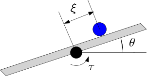
Figure 1: Ball and beam system

$\theta$ is the angle that the beam makes with the horizontal while $\xi$ is the position of the ball on the beam, measured from the beam’s pivot. The beam is actuated by a motor at it’s pivot. The system trajectories evolve over the manifold $Q=S^{1}\times\mathbb{R}$. The beam constitutes the actuated subsystem while the ball constitutes the unactuated subsystem. The Lagrangian of the system is given by

$$\mathcal{L}\ :\ TQ\rightarrow\mathbb{R}$$

$$\mathcal{L}(\xi,\theta,\dot{\xi},\dot{\theta})=\frac{1}{2}I_{r}\dot{\theta}^{2}+\frac{1}{2}m_{b}(\dot{\xi}^{2}+\xi^{2}\dot{\theta}^{2})-m_{b}g\xi\sin\theta$$

We now proceed to discretize the system dynamics using the trapezoidal rule. For a time step $h$, the discrete Lagrangian is given by

$$\mathcal{L}_{dk}\ :\ Q\times Q\rightarrow\mathbb{R}$$

$$\mathcal{L}_{dk}(\xi_{k},\theta_{k},\Delta\xi_{k},\Delta\theta_{k}) =hL(\xi_{k},\theta_{k},\frac{\Delta\xi_{k}}{h},\frac{\Delta\theta_{k}}{h})$$

$$=\frac{1}{2h}I_{r}\Delta\theta_{k}^{2}+\frac{1}{2h}m_{b}(\Delta\xi_{k}^{2}+\xi_{k}^{2}\Delta\theta_{k}^{2})$$

$$-m_{b}hg\xi_{k}\sin\theta_{k}$$

The discrete-time Euler-Lagrange equations of motion are given by

$$\frac{I_{r}}{h}(\Delta\theta_{k-1}-\Delta\theta_{k})+\frac{m_{b}}{h}(\xi^{2}_{k-1}\Delta\theta_{k-1}-\xi^{2}_{k}\Delta\theta_{k})$$

$$-m_{b}hg\xi_{k}\cos\theta_{k}+\frac{h}{2}(u_{k}+u_{k-1})=0$$ (25a)

$$\frac{m_{b}}{h}(\Delta\xi_{k-1}-\Delta\xi_{k})+\frac{m_{b}}{h}(\xi_{k}\Delta\theta_{k}^{2})-m_{b}hg\sin\theta_{k}=0$$ (25b)

$$\theta_{k}=\theta_{k-1}+\Delta\theta_{k-1}$$ (25c)

$$\xi_{k}=\xi_{k-1}+\Delta\xi_{k-1}$$ (25d)

The discrete-time Hamilton’s equations are given by

$$\mu_{ak}=m_{b}hg\xi_{k}\cos\theta_{k}+\frac{I_{r}}{h}\Delta\theta_{k}+\frac{m_{b}}{h}\xi^{2}_{k}\Delta\theta_{k}-\frac{h}{2}u_{k}$$ (26a)

$$\theta_{k+1}=\theta_{k}+\Delta\theta_{k}$$ (26b)

$$\mu_{ak+1}=\mu_{ak}-m_{b}hg\xi_{k}\cos\theta_{k}+\frac{h}{2}u_{k}+\frac{h}{2}u_{k+1}$$ (26c)

$$\mu_{uk}=\frac{m_{b}}{h}\Delta\xi_{k}-\frac{m_{b}}{h}(\xi_{k}\Delta\theta_{k}^{2})+m_{b}hg\sin\theta_{k}$$ (26d)

$$\xi_{k+1}=\xi_{k}+\Delta\xi_{k}$$ (26e)

$$\mu_{uk+1}=\mu_{uk}+\frac{m_{b}}{h}(\xi_{k}\Delta\theta_{k}^{2})-m_{b}hg\sin\theta_{k}$$ (26f)

Let us find the sequence of controls $\{u_{k}\}$ which minimizes the cost $\mathcal{J}_{d}=\sum_{k=0}^{N-1}\frac{1}{2}u^{2}_{k}$ and gets the system from $(\theta_{0},\xi_{0},\mu_{a0},\mu_{u0})=(\theta_{0},\xi_{0},0,0)$ to $(\theta_{N},\xi_{N},\mu_{aN},\mu_{uN})=(\theta_{f},\xi_{f},0,0)$.
We thus wish to solve the problem

$$\textrm{min}_{u_{k}}(\mathcal{J}_{d} =\sum_{k=0}^{N-1}\frac{1}{2}u^{2}_{k})$$

$$\textrm{such that }(\theta_{0},\xi_{0},\mu_{a0},\mu_{u0}) =(\theta_{0},\xi_{0},0,0)$$

$$(\theta_{N},\xi_{N},\mu_{aN},\mu_{uN}) =(\theta_{f},\xi_{f},0,0)$$

$$\textrm{subject to }(\ref{heqbb})$$ (27)

The following table presents the first and second derivatives of the Lagrangian (defined as in (23) and (24)) in order to obtain the multiplier equations and optimality condition as in (19) and (20)

$M_{ag}=-m_{b}gh\xi_{k}\cos\theta_{k}$	$M_{af}=\frac{I_{r}}{h}\Delta\theta_{k}+\frac{m_{b}}{h}\xi^{2}_{k}\Delta\theta_{k}$
$\mathcal{M}^{ag}_{ag}=m_{b}gh\xi_{k}\sin\theta_{k}\lambda$	$\mathcal{M}^{ag}_{af}=0$
$\mathcal{M}^{af}_{ag}=0$	$\mathcal{M}^{af}_{af}=(\frac{I_{r}}{h}+\frac{m_{b}}{h}\xi^{2}_{k})\lambda$
$\mathcal{M}^{ug}_{ag}=-m_{b}gh\cos\theta_{k}\lambda$	$\mathcal{M}^{ug}_{af}=2\frac{m_{b}}{h}\xi_{k}\Delta\theta_{k}\lambda$
$\mathcal{M}^{uf}_{ag}=0$	$\mathcal{M}^{uf}_{af}=0$
$M_{ug}=\frac{m_{b}}{h}\xi_{k}\Delta\theta_{k}^{2}-m_{b}gh\sin\theta_{k}$	$M_{uf}=\frac{m_{b}}{h}\Delta\xi_{k}$
$\mathcal{M}^{ag}_{ug}=-m_{b}gh\cos\theta_{k}\lambda$	$\mathcal{M}^{ag}_{uf}=0$
$\mathcal{M}^{af}_{ug}=2\frac{m_{b}}{h}\xi_{k}\Delta\theta_{k}\lambda$	$\mathcal{M}^{af}_{uf}=0$
$\mathcal{M}^{ug}_{ug}=\frac{m_{b}}{h}\Delta\theta_{k}^{2}\lambda$	$\mathcal{M}^{ug}_{uf}=0$
$\mathcal{M}^{uf}_{ug}=0$	$\mathcal{M}^{uf}_{uf}=\frac{m_{b}}{h}\lambda$

The multiplier equations and condition of optimality are therefore given by

$$m_{b}gh\xi_{k}\sin\theta_{k}(\lambda^{1}_{k}-\lambda^{3}_{k})-m_{b}gh\cos\theta_{k}(\lambda^{4}_{k}-\lambda^{6}_{k})=-\lambda^{2}_{k-1}+\lambda^{2}_{k}$$ (28a)

$$m_{b}gh\cos\theta_{k}(\lambda^{3}_{k}-\lambda^{1}_{k})-2\frac{m_{b}}{h}\xi_{k}\Delta\theta_{k}\lambda^{1}_{k}+\frac{m_{b}}{h}\Delta\theta_{k}^{2}(\lambda^{4}_{k}-\lambda^{6}_{k})$$

$$\hskip 142.26378pt=-\lambda^{5}_{k-1}+\lambda^{5}_{k}$$ (28b)

$$-(\frac{I_{r}}{h}+\frac{m_{b}}{h}\xi^{2}_{k})\lambda^{1}_{k}+2\frac{m_{b}}{h}\xi_{k}\Delta\theta_{k}(\lambda^{4}_{k}-\lambda^{6}_{k})=\lambda^{2}_{k}$$ (28c)

$$-\frac{m_{b}}{h}\lambda^{4}_{k}=\lambda^{5}_{k}$$ (28d)

$$\lambda^{1}_{k}-\lambda^{3}_{k}=-\lambda^{3}_{k-1}$$ (28e)

$$\lambda^{4}_{k}-\lambda^{6}_{k}=-\lambda^{6}_{k-1}$$ (28f)

$$u_{k}+\frac{h}{2}\lambda^{1}_{k}-\frac{h}{2}\lambda^{3}_{k}=\frac{h}{2}\lambda^{3}_{k-1}\hskip 28.45274pt\forall k=1,2,\dots,N-1$$ (28g)

$$u_{0}+\frac{h}{2}\lambda^{1}_{0}-\frac{h}{2}\lambda^{3}_{0}=0$$ (28h)

The above equations are solved using the multiple shooting method described in [13].

Simulation Results

The solution was obtained numerically on a PC by implementing the above algorithm with the following parameters

Parameter	Value
$m_{b}$	$0.5\ kg$
$I_{r}$	$6\ kg\ m^{2}$
$g$	$9.8\ m\ s^{-2}$
$h$	$0.01\ s$
N	1000

We present our results for two sets of boundary conditions

Case 1

The initial and terminal conditions are set as

$\theta_{0}=$	0	$\theta_{N}=$	0
$\mu_{a0}=$	$0\ kg\ m^{2}\ s^{-1}$	$\mu_{aN}=$	$0\ kg\ m^{2}\ s^{-1}$
$\xi_{0}=$	$0.5\ m$	$\xi_{N}=$	$0\ m$
$\mu_{u0}=$	$0\ kg\ m\ s^{-1}$	$\mu_{uN}=$	$0\ kg\ m\ s^{-1}$

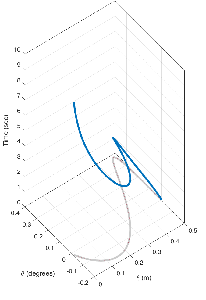
Figure 2: Evolution of ball and beam configurations with time for case 1

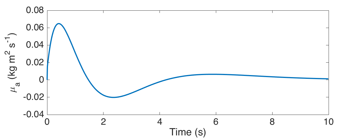
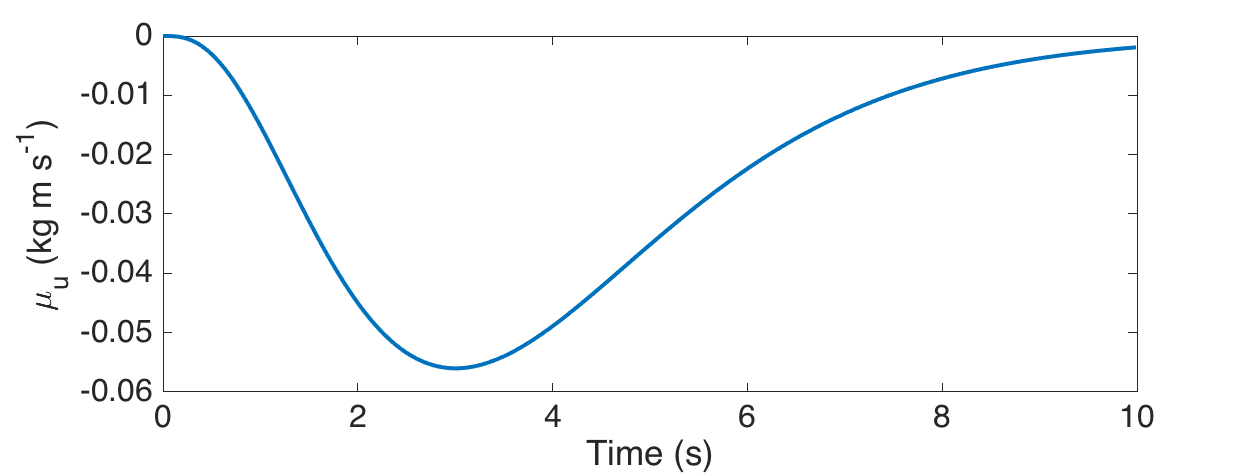
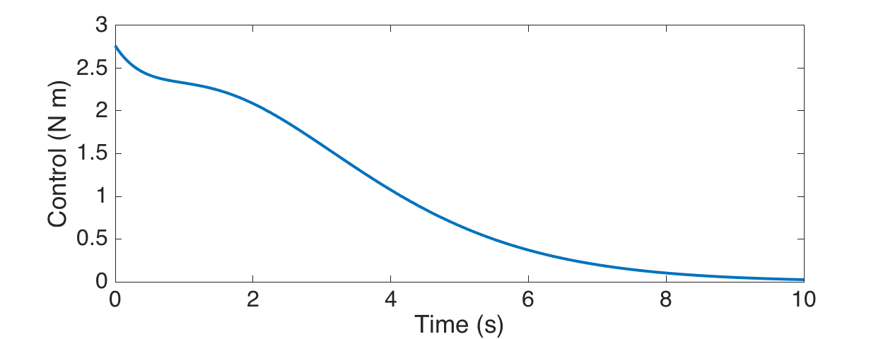
Figure 3: Momenta and control input versus time for case 1

We see that the numerical solution obtained respects the boundary conditions satisfactorily, stabilizing both, the ball and the beam.

Case 2

The initial and terminal conditions are set as

$\theta_{0}=$	$18^{\circ}$	$\theta_{N}=$	0
$\mu_{a0}=$	$0\ kg\ m^{2}\ s^{-1}$	$\mu_{aN}=$	$0\ kg\ m^{2}\ s^{-1}$
$\xi_{0}=$	$0.5\ m$	$\xi_{N}=$	$0\ m$
$\mu_{u0}=$	$0\ kg\ m\ s^{-1}$	$\mu_{uN}=$	$0\ kg\ m\ s^{-1}$

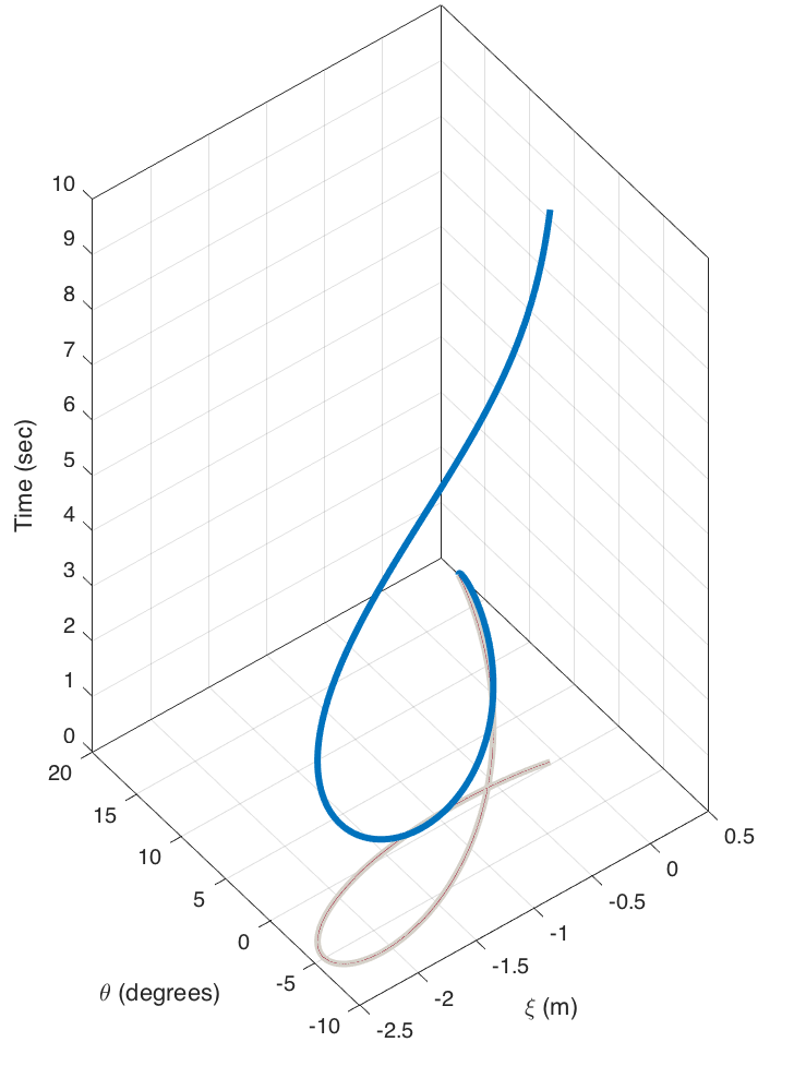
Figure 4: Evolution of ball and beam configurations with time for case 2

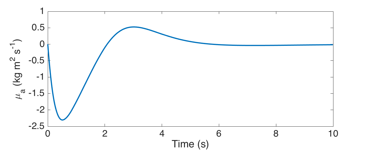
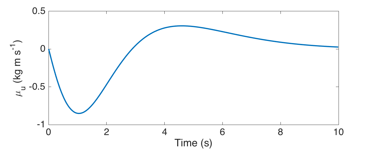
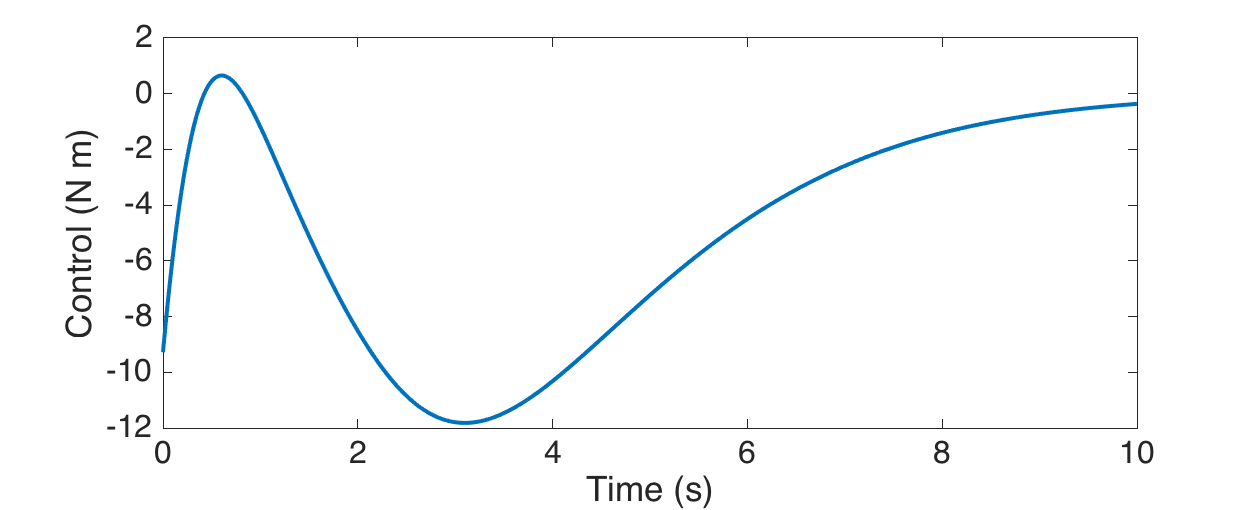
Figure 5: Momenta and control input versus time for case 2

VI EXAMPLE: Inverted Pendulum on a Cart

Consider an inverted pendulum with a bob of mass $m_{b}$ hinged onto a cart of mass $m_{c}$. The situation is described in the figure below.

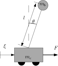
Figure 6: Inverted pendulum on a cart

$\theta$ is the angle that the pendulum makes with the vertical while $\xi$ is the position of the cart. An external force $F$ acting the cart serves as the control input to the system. The system trajectories evolve over the manifold $Q=S^{1}\times\mathbb{R}$ with the pendulum constituting the unactuated subsystem, and the cart constituting the actuated subsystem. The Lagrangian of the system is given by

$$\mathcal{L}\ :\ TQ\rightarrow\mathbb{R}$$

$$\mathcal{L}(\xi,\theta,\dot{\xi},\dot{\theta})=\frac{1}{2}(m_{b}+m_{c})\dot{\xi}^{2}+\frac{1}{2}m_{b}l^{2}\dot{\theta}^{2}-m_{b}l\dot{\xi}\dot{\theta}\cos\theta-m_{b}gl\cos\theta$$

We now proceed to discretize the system dynamics using the trapezoidal rule. For a time step $h$, the discrete Lagrangian is given by

$$\mathcal{L}_{dk}\ :\ Q\times Q\rightarrow\mathbb{R}$$

$$\mathcal{L}_{dk}(\xi_{k},\theta_{k},\Delta\xi_{k},\Delta\theta_{k}) =hL(\xi_{k},\theta_{k},\frac{\Delta\xi_{k}}{h},\frac{\Delta\theta_{k}}{h})$$

$$=\frac{1}{2h}(m_{b}+m_{c})\Delta\xi_{k}^{2}+\frac{1}{2h}m_{b}l^{2}\Delta\theta_{k}^{2}$$

$$-\frac{m_{b}}{h}l\Delta\xi_{k}\Delta\theta_{k}\cos\theta_{k}-m_{b}hgl\cos\theta_{k}$$

The discrete-time Euler-Lagrange equations of motion are given by

$$\frac{m_{b}l^{2}}{h}(\Delta\theta_{k-1}-\Delta\theta_{k})+\frac{m_{b}l}{h}(\Delta\xi_{k}\cos\theta_{k}-\Delta\xi_{k-1}\cos\theta_{k-1})$$

$$+\frac{m_{b}l}{h}\Delta\xi_{k}\Delta\theta_{k}\sin\theta_{k}+m_{b}glh\sin\theta_{k}=0$$ (29a)

$$\frac{m_{b}+m_{c}}{h}(\Delta\xi_{k-1}-\Delta\xi_{k})+\frac{m_{b}l}{h}(\Delta\theta_{k}\cos\theta_{k}-\Delta\theta_{k-1}\cos\theta_{k-1})$$

$$+\frac{h}{2}(F_{k}+F_{k-1})=0$$ (29b)

$$\theta_{k}=\theta_{k-1}+\Delta\theta_{k-1}$$ (29c)

$$\xi_{k}=\xi_{k-1}+\Delta\xi_{k-1}$$ (29d)

The discrete-time Hamilton’s equations are given by

$$\mu_{ak}=\frac{m_{b}+m_{c}}{h}\Delta\xi_{k}-\frac{m_{b}l}{h}\Delta\theta_{k}\cos\theta_{k}-\frac{h}{2}F_{k}$$ (30a)

$$\xi_{k+1}=\xi_{k}+\Delta\xi_{k}$$ (30b)

$$\mu_{ak+1}=\mu_{ak}+\frac{h}{2}F_{k}+\frac{h}{2}F_{k+1}$$ (30c)

$$\mu_{uk}=-m_{b}ghl\sin\theta_{k}-\frac{m_{b}l}{h}\Delta\xi_{k}\Delta\theta_{k}\sin\theta_{k}+\frac{m_{b}l}{h}(l\Delta\theta_{k}-\Delta\xi_{k}\cos\theta_{k})$$ (30d)

$$\theta_{k+1}=\theta_{k}+\Delta\theta_{k}$$ (30e)

$$\mu_{uk+1}=\mu_{uk}+\frac{m_{b}l}{h}\Delta\xi_{k}\Delta\theta_{k}\sin\theta_{k}+m_{b}glh\sin\theta_{k}$$ (30f)

Let us find the sequence of controls $\{u_{k}\}$ which minimizes the cost $\mathcal{J}_{d}=\sum_{k=0}^{N-1}\frac{1}{2}u^{2}_{k}$ and gets the system from $(\theta_{0},\xi_{0},\mu_{a0},\mu_{u0})=(\theta_{0},\xi_{0},0,0)$ to $(\theta_{N},\xi_{N},\mu_{aN},\mu_{uN})=(\theta_{f},\xi_{f},0,0)$.

We thus wish to solve the problem

$$\textrm{min}_{u_{k}}(\mathcal{J}_{d} =\sum_{k=0}^{N-1}\frac{1}{2}u^{2}_{k})$$

$$\textrm{such that }(\theta_{0},\xi_{0},\mu_{a0},\mu_{u0}) =(\theta_{0},\xi_{0},0,0)$$

$$(\theta_{N},\xi_{N},\mu_{aN},\mu_{uN}) =(\theta_{f},\xi_{f},0,0)$$

$$\textrm{subject to }(\ref{heqbb})$$ (31)

The following table presents the first and second derivatives of the Lagrangian (defined as in (23) and (24)) in order to obtain the multiplier equations and optimality condition as in (19) and (20)

$M_{ag}=0$	$M_{af}=\frac{m_{b}+m_{c}}{h}\Delta\xi_{k}$
	$-\frac{m_{b}l}{h}\Delta\theta_{k}\cos\theta_{k}$
$\mathcal{M}^{ag}_{ag}=0$	$\mathcal{M}^{ag}_{af}=0$
$\mathcal{M}^{af}_{ag}=0$	$\mathcal{M}^{af}_{af}=\frac{m_{b}+m_{c}}{h}\lambda$
$\mathcal{M}^{ug}_{ag}=0$	$\mathcal{M}^{ug}_{af}=\frac{m_{b}l}{h}\Delta\theta_{k}\sin\theta_{k}\lambda$
$\mathcal{M}^{uf}_{ag}=0$	$\mathcal{M}^{uf}_{af}=-\frac{m_{b}l}{h}\cos\theta_{k}\lambda$
$M_{ug}=\frac{m_{b}l}{h}\Delta\xi_{k}\Delta\theta_{k}\sin\theta_{k}$	$M_{uf}=\frac{m_{b}l^{2}}{h}\Delta\theta_{k}$
$+m_{b}hgl\sin\theta_{k}$	$-\frac{m_{b}l}{h}\Delta\xi_{k}\cos\theta_{k}$
$\mathcal{M}^{ag}_{ug}=0$	$\mathcal{M}^{ag}_{uf}=0$
$\mathcal{M}^{af}_{ug}=\frac{m_{b}l}{h}\Delta\theta_{k}\sin\theta_{k}\lambda$	$\mathcal{M}^{af}_{uf}=-\frac{m_{b}l}{h}\cos\theta_{k}\lambda$
$\mathcal{M}^{ug}_{ug}=\frac{m_{b}l}{h}\Delta\xi_{k}\Delta\theta_{k}\cos\theta_{k}\lambda$	$\mathcal{M}^{ug}_{uf}=\frac{m_{b}l}{h}\Delta\xi_{k}\sin\theta_{k}\lambda$
$+m_{b}hgl\sin\theta_{k}\lambda$
$\mathcal{M}^{uf}_{ug}=\frac{m_{b}l}{h}\Delta\xi_{k}\sin\theta_{k}\lambda$	$\mathcal{M}^{uf}_{uf}=\frac{m_{b}l^{2}}{h}\lambda$

The multiplier equations and condition of optimality are therefore given by

$$0=-\lambda^{2}_{k-1}+\lambda^{2}_{k}$$ (32a)

$$-\frac{m_{b}l}{h}\Delta\theta_{k}\sin\theta\lambda^{1}_{k}-\frac{m_{b}l}{h}\Delta\xi_{k}\sin\theta_{k}\lambda^{4}_{k}$$

$$+\frac{m_{b}l}{h}\Delta\xi_{k}\Delta\theta_{k}\cos\theta_{k}(\lambda^{4}_{k}-\lambda^{6}_{k})+m_{b}hgl\sin\theta_{k}(\lambda^{4}_{k}-\lambda^{6}_{k})$$

$$=-\lambda^{5}_{k-1}+\lambda^{5}_{k}$$ (32b)

$$-\frac{m_{b}+m_{c}}{h}\lambda^{1}_{k}+\frac{m_{b}l}{h}\Delta\theta_{k}\sin\theta_{k}(\lambda^{4}_{k}-\lambda^{6}_{k})+\frac{m_{b}l}{h}\cos\theta_{k}\lambda^{4}_{k}$$

$$=\lambda^{2}_{k}$$ (32c)

$$\frac{m_{b}l}{h}\cos\theta_{k}\lambda^{1}_{k}+\frac{m_{b}l}{h}\Delta\xi_{k}\sin\theta_{k}(\lambda^{4}_{k}-\lambda^{6}_{k})-\frac{m_{b}l^{2}}{h}\lambda^{4}_{k}=\lambda^{5}_{k}$$ (32d)

$$\lambda^{1}_{k}-\lambda^{3}_{k}=-\lambda^{3}_{k-1}$$ (32e)

$$\lambda^{4}_{k}-\lambda^{6}_{k}=-\lambda^{6}_{k-1}$$ (32f)

$$F_{k}+\frac{h}{2}\lambda^{1}_{k}-\frac{h}{2}\lambda^{3}_{k}=\frac{h}{2}\lambda^{3}_{k-1}\hskip 28.45274pt\forall k=1,2,\dots,N-1$$ (32g)

$$F_{0}+\frac{h}{2}\lambda^{1}_{0}-\frac{h}{2}\lambda^{3}_{0}=0$$ (32h)

The solutions to these equations are also solved using the multiple shooting method described in [13].

Simulation Results

As in the previous example, we obtain the solution numerically on a PC by implementing the above algorithm with the following parameters

Parameter	Value
$m_{c}$	$0.5\ kg$
$m_{b}$	$0.1\ kg$
$l$	$0.1\ m$
$g$	$9.8\ m\ s^{-2}$
$h$	$0.01\ s$
N	1000

We present our results for two sets of boundary conditions

Case 1

The initial and terminal conditions are set as

$\theta_{0}=$	$60^{\circ}$	$\theta_{N}=$	0
$\mu_{a0}=$	$0\ kg\ m^{2}\ s^{-1}$	$\mu_{aN}=$	$0\ kg\ m^{2}\ s^{-1}$
$\xi_{0}=$	$2\ m$	$\xi_{N}=$	$0\ m$
$\mu_{u0}=$	$0\ kg\ m\ s^{-1}$	$\mu_{uN}=$	$0\ kg\ m\ s^{-1}$

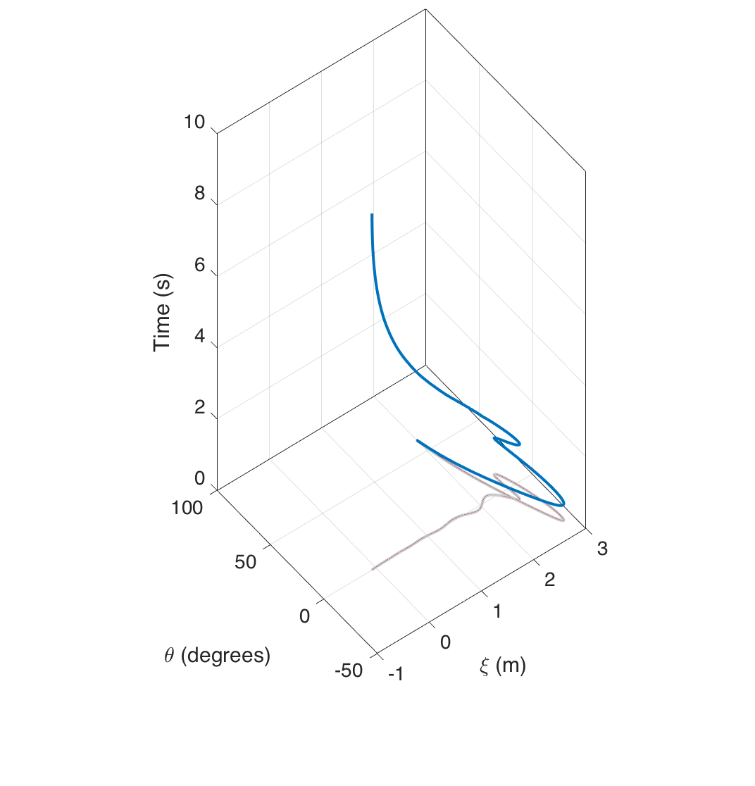
Figure 7: Evolution of pendulum and cart configurations with time for case 1

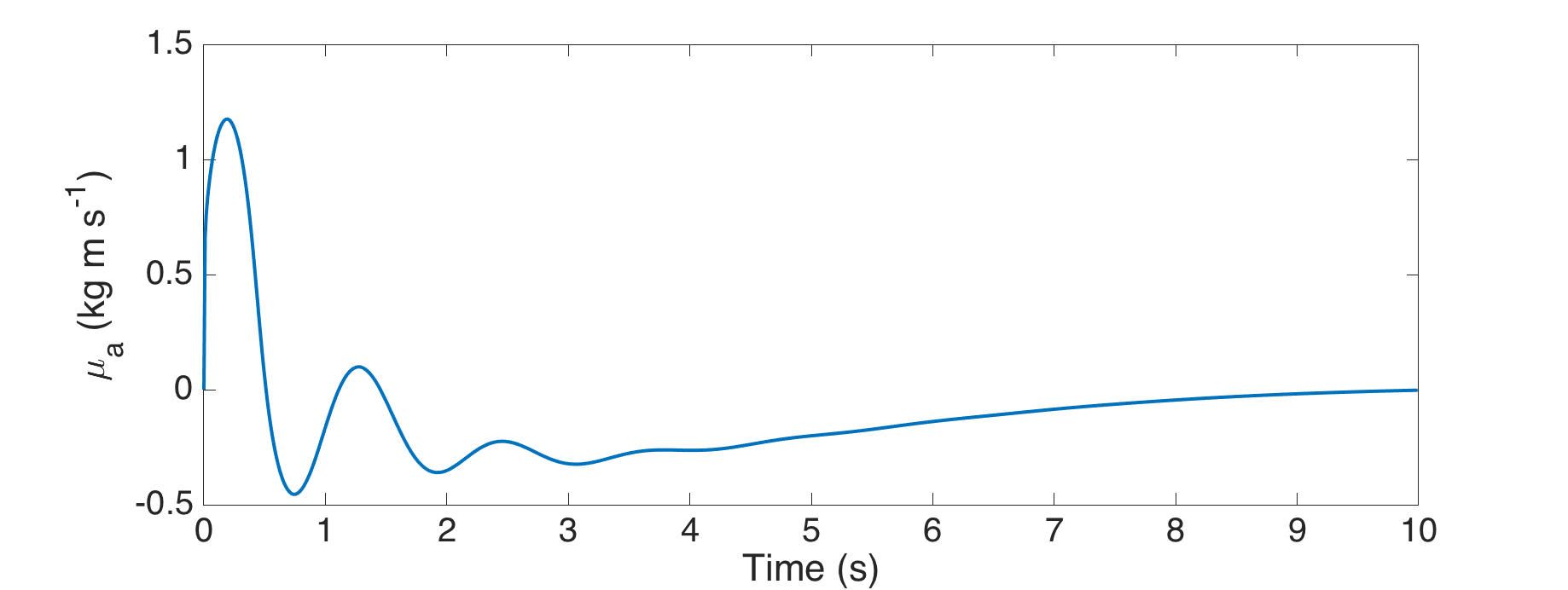
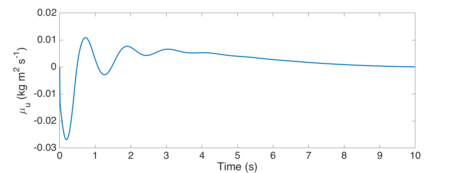
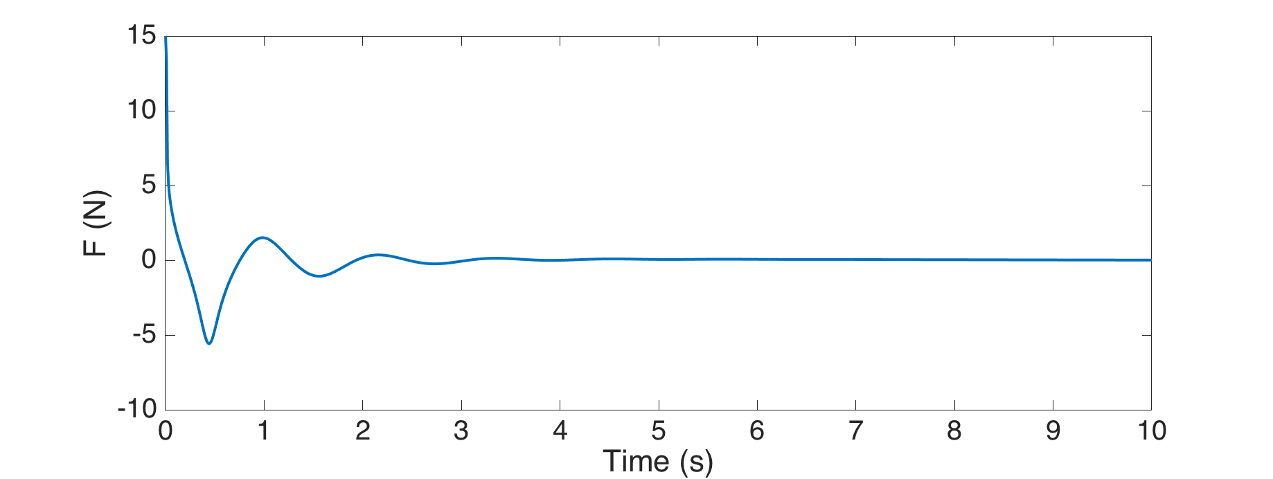
Figure 8: Momenta and control input versus time for case 1

We see that the numerical solution obtained respects the boundary conditions satisfactorily, stabilizing both, the ball and the beam.

Case 2

The initial and terminal conditions are set as

$\theta_{0}=$	$-45^{\circ}$	$\theta_{N}=$	0
$\mu_{a0}=$	$0\ kg\ m^{2}\ s^{-1}$	$\mu_{aN}=$	$0\ kg\ m^{2}\ s^{-1}$
$\xi_{0}=$	$2\ m$	$\xi_{N}=$	$0\ m$
$\mu_{u0}=$	$0\ kg\ m\ s^{-1}$	$\mu_{uN}=$	$0\ kg\ m\ s^{-1}$

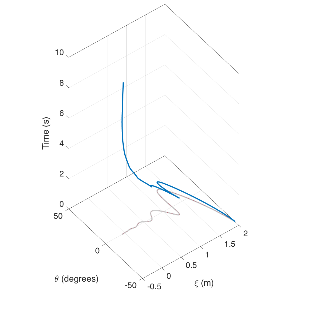
Figure 9: Evolution of pendulum and cart configurations with time for case 2

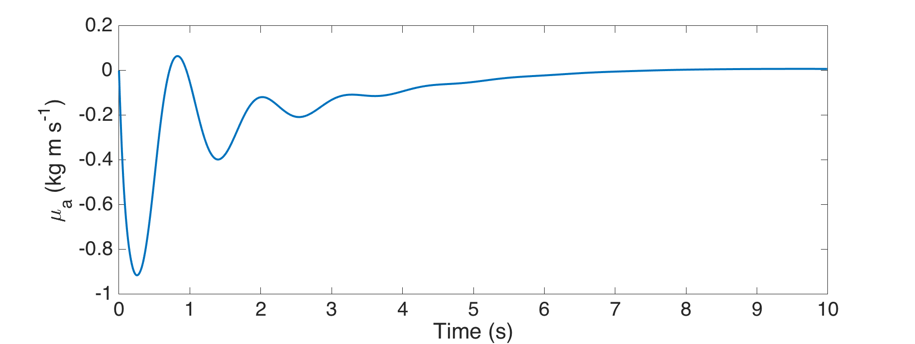
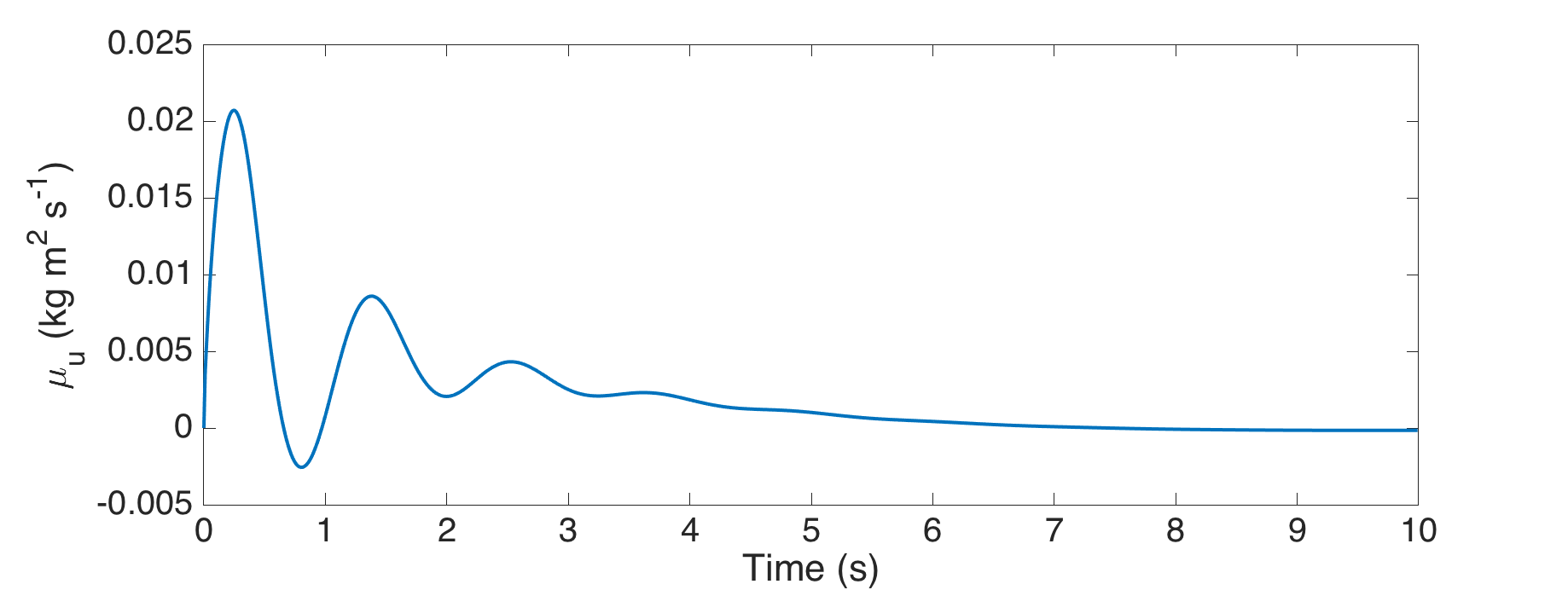
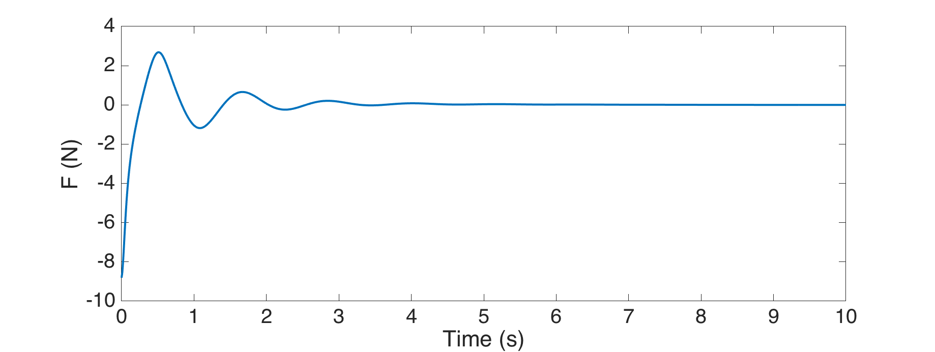
Figure 10: Momenta and control input versus time for case 2

VII Conclusion

In this article, we developed a variational integrator for interconnected mechanical systems evolving on a product of matrix Lie groups. A discrete optimal control problem was formulated for the considered class of systems and subsequently solved using calculus of variations to obtain necessary conditions describing optimal trajectories. The proposed approach is demonstrated on a benchmark underactuated system with satisfactory results. The discrete optimal control problem solved here is that of finding an optimal trajectory, given fixed endpoints. An extension of this work would to be solve a more general class of problems. Moreover, the conditions of optimality obtained in this work are merely necessary conditions that an optimal trajectory should possess. The existence of the same is not guaranteed. A starting attempt to answer this question would be to analyse the controllability of interconnected mechanical systems considered here.

VIII APPENDIX

Obtaining the necessary conditions

With the introduction of Lagrange multipliers, $\mu_{ak},\mu_{uk},g_{uk},g_{ak},f_{uk},f_{ak}$ are varied independently. Using one-parameter subgroups on their respective Lie groups, the variations of the last four terms are given by

$$\delta g_{uk}=g_{uk}\eta_{uk}\quad\delta g_{ak}=g_{ak}\eta_{ak}$$

$$\delta f_{uk}=f_{uk}\chi_{uk}\quad\delta f_{ak}=f_{ak}\chi_{ak}$$

for some $\eta_{uk},\chi_{uk}\ \in\mathfrak{g}_{u}$ and $\eta_{ak},\chi_{ak}\in\mathfrak{g}_{a}$. We’ll require the following results to calculate the variations of the terms in (16).
For $g\in G$, the adjoint operator $\textrm{Ad}_{g}:\mathfrak{g}\rightarrow\mathfrak{g}$ is the tangent lift of the inner automorphism

$$\textrm{Ad}_{g}\xi=T_{g^{-1}}L_{g}\cdot T_{e}R_{g^{-1}}\cdot\xi$$ (33)

The derivative of $\textrm{Ad}_{g}\xi$ with respect to $g$ at $e$ in the direction $\eta$ gives us the ad operator $\textrm{ad}_{\eta}\xi=[\eta,\xi]$

$$\left.\dfrac{d}{d\epsilon}\right|_{\epsilon=0}\textrm{Ad}_{\textrm{exp}\ \epsilon\eta}\xi=[\eta,\xi]$$ (34)

Proposition 1

The derivatives of the $Ad$ map are given by

$$\left.\dfrac{d}{d\epsilon}\right|_{\epsilon=0}\textrm{Ad}_{g\exp{\ \epsilon\eta}}\xi=\textrm{Ad}_{g}[\eta,\xi]=[\textrm{Ad}_{g}\eta,\textrm{Ad}_{g}\xi]$$ (35a)

$$\left.\dfrac{d}{d\epsilon}\right|_{\epsilon=0}\textrm{Ad}_{(g\exp{\ \epsilon\eta})^{-1}}\xi=[\textrm{Ad}_{g^{-1}}\xi,\eta]$$ (35b)

$$\left.\dfrac{d}{d\epsilon}\right|_{\epsilon=0}\textrm{Ad}^{*}_{g\exp{\ \epsilon\eta}}\alpha=\textrm{Ad}^{*}_{g}(\textrm{ad}^{*}_{\textrm{Ad}_{g}\eta}\alpha)$$ (35c)

$$\left.\dfrac{d}{d\epsilon}\right|_{\epsilon=0}\textrm{Ad}^{*}_{(g\exp{\ \epsilon\eta})^{-1}}\alpha=-\textrm{Ad}^{*}_{g^{-1}}(\textrm{ad}^{*}_{\eta}\alpha)$$ (35d)

Proof:

$$\left.\dfrac{d}{d\epsilon}\right|_{\epsilon=0}\textrm{Ad}_{g\exp{\ \epsilon\eta}}\xi =\left.\dfrac{d}{d\epsilon}\right|_{\epsilon=0}\textrm{Ad}_{g}\circ\textrm{Ad}_{\exp{\ \epsilon\eta}}\xi$$

$$=\textrm{Ad}_{g}[\eta,\xi]$$

$$=[\textrm{Ad}_{g}\eta,\textrm{Ad}_{g}\xi]$$

$$\left.\dfrac{d}{d\epsilon}\right|_{\epsilon=0}\textrm{Ad}_{(g\exp{\ \epsilon\eta})^{-1}}\xi =\left.\dfrac{d}{d\epsilon}\right|_{\epsilon=0}\textrm{Ad}_{\exp{-\epsilon\eta}}\circ\textrm{Ad}_{g^{-1}}\xi$$

$$=-[\eta,\textrm{Ad}_{g^{-1}}\xi]$$

$$=[\textrm{Ad}_{g^{-1}}\xi,\eta]$$

$$\langle\left.\dfrac{d}{d\epsilon}\right|_{\epsilon=0}\textrm{Ad}^{*}_{g\exp{\ \epsilon\eta}}\alpha,\xi\rangle =\langle\alpha,\left.\dfrac{d}{d\epsilon}\right|_{\epsilon=0}\textrm{Ad}_{g\exp{\ \epsilon\eta}}\xi\rangle$$

$$=\langle\alpha,[\textrm{Ad}_{g}\eta,\textrm{Ad}_{g}\xi]\rangle$$

$$=\langle\alpha,\textrm{ad}_{\textrm{Ad}_{g}\eta}(\textrm{Ad}_{g}\xi)\rangle$$

$$=\langle\textrm{Ad}^{*}_{g}(\textrm{ad}^{*}_{\textrm{Ad}_{g}\eta}\alpha),\xi\rangle$$

$$\langle\left.\dfrac{d}{d\epsilon}\right|_{\epsilon=0}\textrm{Ad}^{*}_{(g\exp{\ \epsilon\eta})^{-1}}\alpha,\xi\rangle =\langle\alpha,\left.\dfrac{d}{d\epsilon}\right|_{\epsilon=0}\textrm{Ad}_{(g\exp{\ \epsilon\eta})^{-1}}\xi\rangle$$

$$=\langle\alpha,-[\eta,\textrm{Ad}_{g^{-1}}\xi]\rangle$$

$$=\langle\alpha,-\textrm{ad}_{\eta}(\textrm{Ad}_{g^{-1}}\xi)\rangle$$

$$=\langle-\textrm{Ad}^{*}_{g^{-1}}(\textrm{ad}^{*}_{\eta}\alpha),\xi\rangle$$

$\blacksquare$

Now we proceed to obtain the variations of the terms in (16)

$$\delta\mathcal{J}_{d0} =D_{g_{ak}}\phi_{d}(g_{k},f_{k},u_{k})\cdot\delta g_{ak}+D_{g_{uk}}\phi_{d}(g_{k},f_{k},u_{k})\cdot\delta g_{uk}$$

$$+D_{f_{ak}}\phi_{d}(g_{k},f_{k},u_{k})\cdot\delta f_{ak}+D_{f_{uk}}\phi_{d}(g_{k},f_{k},u_{k})\cdot\delta f_{uk}$$

$$+D_{u_{k}}\phi_{d}(g_{k},f_{k},u_{k})\cdot\delta u_{k}$$

$$=\langle T^{*}_{e}L_{g_{ak}}\cdot D_{g_{ak}}\phi_{d},\eta_{ak}\rangle+\langle T^{*}_{e}L_{g_{uk}}\cdot D_{g_{uk}}\phi_{d},\eta_{uk}\rangle$$

$$+\langle T^{*}_{e}L_{f_{ak}}\cdot D_{f_{ak}}\phi_{d},\chi_{ak}\rangle+\langle T^{*}_{e}L_{f_{uk}}\cdot D_{f_{uk}}\phi_{d},\chi_{uk}\rangle$$

$$+\langle\delta u_{k},D_{u_{k}}\phi_{d}(g_{k},f_{k},u_{k})\rangle$$

$$\delta\mathcal{J}_{d1} =\delta(\langle\mu_{ak}-(-M_{ag}+\textrm{Ad}^{*}_{f^{-1}_{ak}}\cdot(M_{af})-\frac{1}{2}hu_{k}),\lambda^{1}_{k}\rangle)$$

$$=\langle\delta\mu_{ak}+\frac{h}{2}\delta u_{k}+D_{g_{ak}}M_{ag}\cdot\delta g_{ak}+D_{g_{uk}}M_{ag}\cdot\delta g_{uk}+D_{f_{ak}}M_{ag}\cdot\delta f_{ak}$$

$$+D_{f_{uk}}M_{ag}\cdot\delta f_{uk},\lambda^{1}_{k}\rangle+\langle-\textrm{Ad}^{*}_{f^{-1}_{ak}}(D_{g_{ak}}M_{af}\cdot\delta g_{ak}+D_{g_{uk}}M_{af}\cdot\delta g_{uk}$$

$$+D_{f_{ak}}M_{af}\cdot\delta f_{ak}+D_{f_{uk}}M_{af}\cdot\delta f_{uk})+\textrm{Ad}^{*}_{f_{ak}^{-1}}(\textrm{ad}^{*}_{\chi_{ak}}M_{af}),\lambda^{1}_{k}\rangle$$

$$=\langle\mathcal{M}^{ag}_{ag}(\lambda^{1}_{k})-\mathcal{M}^{ag}_{af}(\textrm{Ad}_{f^{-1}_{ak}}\lambda^{1}_{k}),\eta_{ak}\rangle+\langle\mathcal{M}^{ug}_{ag}(\lambda^{1}_{k})-\mathcal{M}^{ug}_{af}(\textrm{Ad}_{f^{-1}_{ak}}\lambda^{1}_{k}),\eta_{uk}\rangle$$

$$+\langle\mathcal{M}^{af}_{ag}(\lambda^{1}_{k})-\mathcal{M}^{af}_{af}(\textrm{Ad}_{f^{-1}_{ak}}\lambda^{1}_{k}),\chi_{ak}\rangle+\langle\mathcal{M}^{uf}_{ag}(\lambda^{1}_{k})-\mathcal{M}^{uf}_{af}(\textrm{Ad}_{f^{-1}_{ak}}\lambda^{1}_{k}),\chi_{uk}\rangle$$

$$+\langle-\textrm{ad}^{*}_{\textrm{Ad}_{f_{ak}^{-1}}\lambda^{1}_{k}}(M_{af}),\chi_{ak}\rangle+\langle\delta\mu_{ak}+\frac{h}{2}\delta u_{k},\lambda^{1}_{k}\rangle$$

$$\delta\mathcal{J}_{d3} =\delta(\langle\mu_{ak+1}-(\textrm{Ad}^{*}_{f_{ak}}(\mu_{ak}+M_{ag}+\frac{1}{2}hu_{k})+\frac{1}{2}hu_{k+1}),\lambda^{3}_{k}\rangle)$$

$$=\langle\delta\mu_{ak+1}-\frac{h}{2}\delta u_{k+1}-\textrm{Ad}^{*}_{f_{ak}}(\delta\mu_{ak}+\frac{h}{2}\delta u_{k}+\textrm{ad}^{*}_{\textrm{Ad}_{f_{ak}}\chi_{ak}}M_{ag}),\lambda^{3}_{k}\rangle$$

$$+\langle-\textrm{Ad}^{*}_{f_{ak}}(D_{g_{ak}}M_{ag}\cdot\delta g_{ak}+D_{g_{uk}}M_{ag}\cdot\delta g_{uk}+D_{f_{ak}}M_{ag}\cdot\delta f_{ak}$$

$$+D_{f_{uk}}M_{ag}\cdot\delta f_{uk}),\lambda^{3}_{k}\rangle$$

$$=\langle\delta\mu_{ak+1},\lambda^{3}_{k}\rangle-\langle\delta\mu_{ak},\textrm{Ad}_{f_{ak}}\lambda^{3}_{k}\rangle-\langle\delta u_{k},\frac{h}{2}\textrm{Ad}_{f_{ak}}\lambda^{3}_{k}\rangle-\langle\delta u_{k+1},\frac{h}{2}\lambda^{3}_{k}\rangle$$

$$+\langle\textrm{Ad}^{*}_{f_{ak}}\textrm{ad}^{*}_{\textrm{Ad}_{f_{ak}}\lambda^{3}_{k}}(\mu_{ak}+M_{ag}+\frac{1}{2}hu_{k}),\chi_{ak}\rangle-\langle\mathcal{M}^{ag}_{ag}(\textrm{Ad}_{f_{ak}}\lambda^{3}_{k}),\eta_{ak}\rangle$$

$$-\langle\mathcal{M}^{ug}_{ag}(\textrm{Ad}_{f_{ak}}\lambda^{3}_{k}),\eta_{uk}\rangle-\langle\mathcal{M}^{af}_{ag}(\textrm{Ad}_{f_{ak}}\lambda^{3}_{k}),\chi_{ak}\rangle-\langle\mathcal{M}^{uf}_{ag}(\textrm{Ad}_{f_{ak}}\lambda^{3}_{k}),\chi_{uk}\rangle$$

$$\delta\mathcal{J}_{d4} =\delta(\langle\mu_{uk}-(-M_{ug}+\textrm{Ad}^{*}_{f^{-1}_{uk}}\cdot(M_{uf})),\lambda^{4}_{k}\rangle)$$

$$=\langle\delta\mu_{uk}+D_{g_{ak}}M_{ug}\cdot\delta g_{ak}+D_{g_{uk}}M_{ug}\cdot\delta g_{uk}+D_{f_{ak}}M_{ug}\cdot\delta f_{ak}$$

$$+D_{f_{uk}}M_{ug}\cdot\delta f_{uk},\lambda^{4}_{k}\rangle+\langle-\textrm{Ad}^{*}_{f^{-1}_{uk}}(D_{g_{ak}}M_{uf}\cdot\delta g_{ak}+D_{g_{uk}}M_{uf}\cdot\delta g_{uk}$$

$$+D_{f_{ak}}M_{uf}\cdot\delta f_{ak}+D_{f_{uk}}M_{uf}\cdot\delta f_{uk})+\textrm{Ad}^{*}_{f_{uk}^{-1}}(\textrm{ad}^{*}_{\chi_{uk}}M_{uf}),\lambda^{4}_{k}\rangle$$

$$=\langle\mathcal{M}^{ag}_{ug}(\lambda^{4}_{k})-\mathcal{M}^{ag}_{uf}(\textrm{Ad}_{f^{-1}_{uk}}\lambda^{4}_{k}),\eta_{ak}\rangle$$

$$+\langle\mathcal{M}^{ug}_{ug}(\lambda^{4}_{k})-\mathcal{M}^{ug}_{uf}(\textrm{Ad}_{f^{-1}_{uk}}\lambda^{4}_{k}),\eta_{uk}\rangle$$

$$+\langle\mathcal{M}^{af}_{ug}(\lambda^{4}_{k})-\mathcal{M}^{af}_{uf}(\textrm{Ad}_{f^{-1}_{uk}}\lambda^{4}_{k}),\chi_{ak}\rangle$$

$$+\langle\mathcal{M}^{uf}_{ug}(\lambda^{4}_{k})-\mathcal{M}^{uf}_{uf}(\textrm{Ad}_{f^{-1}_{uk}}\lambda^{4}_{k}),\chi_{uk}\rangle+\langle-\textrm{ad}^{*}_{\textrm{Ad}_{f_{uk}^{-1}}\lambda^{4}_{k}}(M_{uf}),\chi_{uk}\rangle$$

$$+\langle\delta\mu_{uk},\lambda^{4}_{k}\rangle$$

$$\delta\mathcal{J}_{d6} =\delta(\langle\mu_{uk+1}-(\textrm{Ad}^{*}_{f_{uk}}(\mu_{uk}+M_{ug})),\lambda^{6}_{k}\rangle)$$

$$=\langle\delta\mu_{uk+1}-\textrm{Ad}^{*}_{f_{uk}}(\delta\mu_{uk}+D_{g_{ak}}M_{ug}\cdot\delta g_{ak}+D_{g_{uk}}M_{ug}\cdot\delta g_{uk}$$

$$+D_{f_{ak}}M_{ug}\cdot\delta f_{ak}+D_{f_{uk}}M_{ug}\cdot\delta f_{uk})$$

$$-\textrm{Ad}^{*}_{f_{uk}}\textrm{ad}^{*}_{\textrm{Ad}_{f_{uk}}\chi_{uk}}(\mu_{uk}+M_{ug}),\lambda^{6}_{k}\rangle$$

$$=\langle\delta\mu_{uk+1},\lambda^{6}_{k}\rangle+\langle\delta\mu_{uk},-\textrm{Ad}_{f_{uk}}\lambda^{6}_{k}\rangle$$

$$+\langle\textrm{Ad}^{*}_{f_{uk}}\textrm{ad}^{*}_{\textrm{Ad}_{f_{uk}}\lambda^{6}_{k}}(\mu_{uk}+M_{ug}),\chi_{uk}\rangle-\langle\mathcal{M}^{ag}_{ug}(\textrm{Ad}_{f_{uk}}\lambda^{6}_{k}),\eta_{ak}\rangle$$

$$-\langle\mathcal{M}^{ug}_{ug}(\textrm{Ad}_{f_{uk}}\lambda^{6}_{k}),\eta_{uk}\rangle-\langle\mathcal{M}^{af}_{ug}(\textrm{Ad}_{f_{uk}}\lambda^{6}_{k}),\chi_{ak}\rangle$$

$$-\langle\mathcal{M}^{uf}_{ug}(\textrm{Ad}_{f_{uk}}\lambda^{6}_{k}),\chi_{uk}\rangle$$

Now we compute the variations of the log terms using the BCH formula.

$$\textrm{log}(g^{\epsilon-1}_{uk}g^{\epsilon}_{uk+1}) =\textrm{log}(\exp(-\epsilon\eta_{uk})g^{-1}_{uk}g_{uk+1}\exp(\epsilon\eta_{uk+1}))$$

$$=\log(\exp(-\epsilon\eta_{uk})f_{uk}\exp(\epsilon\eta_{uk+1}))$$

$$=\log(f^{-1}_{uk}\exp(-\epsilon\textrm{Ad}_{f^{-1}_{uk}}\eta_{uk})\exp(\epsilon\eta_{uk+1}))$$

Setting

$$\log(f^{-1}_{uk})=X_{uk}$$

$$\log(\exp(-\epsilon\textrm{Ad}_{f^{-1}_{uk}}\eta_{uk})\exp(\epsilon\eta_{uk+1}))=Y_{uk},$$

the equation can now be written as

$$\textrm{log}(g^{\epsilon-1}_{uk}g^{\epsilon}_{uk+1}) =X_{uk}+\dfrac{\textrm{ad}_{X_{uk}}\exp(\textrm{ad}_{X_{uk}})}{\exp(\textrm{ad}_{X_{uk}})-1}Y_{uk}+O(Y^{2}_{uk})$$

Using the definition of a variation, we obtain the following expression. Formula (17) is used for expanding $\textrm{log}(g^{\epsilon-1}_{uk}g^{\epsilon}_{uk+1})$ while formula (IV) is used to expand $Y_{uk}$.

$$\delta\textrm{log}(g^{\epsilon-1}_{uk}g^{\epsilon}_{uk+1}) =\left.\dfrac{d}{d\epsilon}\right|_{\epsilon=0}\textrm{log}(g^{\epsilon-1}_{uk}g^{\epsilon}_{uk+1})$$

$$=\left.\dfrac{d}{d\epsilon}\right|_{\epsilon=0}X_{uk}+\dfrac{\textrm{ad}_{X_{uk}}\exp(\textrm{ad}_{X_{uk}})}{\exp(\textrm{ad}_{X_{uk}})-1}Y_{uk}+O(Y^{2}_{uk})$$

$$=\left.\dfrac{d}{d\epsilon}\right|_{\epsilon=0}X_{uk}+\dfrac{\textrm{ad}_{X_{uk}}\exp(\textrm{ad}_{X_{uk}})}{\exp(\textrm{ad}_{X_{uk}})-1}(-\epsilon\textrm{Ad}_{f^{-1}_{uk}}\eta_{uk}$$

$$+\epsilon\eta_{uk+1}+O(\epsilon^{2}))+O(\epsilon^{4})$$

$$=\dfrac{\textrm{ad}_{X_{uk}}\exp(\textrm{ad}_{X_{uk}})}{\exp(\textrm{ad}_{X_{uk}})-1}(\eta_{uk+1}-\textrm{Ad}_{f^{-1}_{uk}}\eta_{uk})$$

Similarly,

$$\delta(-\log(f^{\epsilon}_{uk})) =\left.\dfrac{d}{d\epsilon}\right|_{\epsilon=0}\log(\exp(-\epsilon\chi_{uk})f^{-1}_{uk})$$

$$=\dfrac{\textrm{ad}_{X_{uk}}\exp(\textrm{ad}_{X_{uk}})}{\exp(\textrm{ad}_{X_{uk}})-1}(-\chi_{uk})$$

This helps us obtain the variations of $\mathcal{J}_{d2}$ and $\mathcal{J}_{d5}$ as follows

$$\delta\mathcal{J}_{d2} =\langle\lambda^{2}_{k},\dfrac{\textrm{ad}_{X_{ak}}\exp(\textrm{ad}_{X_{ak}})}{\exp(\textrm{ad}_{X_{ak}})-1}(\eta_{ak+1}-\textrm{Ad}_{f^{-1}_{ak}}\eta_{ak}-\chi_{ak})\rangle$$

$$\textrm{Setting }\lambda^{2}_{k}\equiv\left(\dfrac{\textrm{ad}_{X_{ak}}\exp(\textrm{ad}_{X_{ak}})}{\exp(\textrm{ad}_{X_{ak}})-1}\right)^{*}\lambda^{2}_{k},$$

$$=\langle\lambda^{2}_{k},\eta_{ak+1}-\textrm{Ad}_{f^{-1}_{ak}}\eta_{ak}-\chi_{ak}\rangle$$

$$=\langle\lambda^{2}_{k},\eta_{ak+1}\rangle+\langle-\textrm{Ad}^{*}_{f^{-1}_{ak}}\lambda^{2}_{k},\eta_{ak}\rangle+\langle-\lambda^{2}_{k},\chi_{ak}\rangle$$

$$\delta\mathcal{J}_{d5} =\langle\lambda^{5}_{k},\dfrac{\textrm{ad}_{X_{uk}}\exp(\textrm{ad}_{X_{uk}})}{\exp(\textrm{ad}_{X_{uk}})-1}(\eta_{uk+1}-\textrm{Ad}_{f^{-1}_{uk}}\eta_{uk}-\chi_{uk})\rangle$$

$$\textrm{Setting }\lambda^{5}_{k}\equiv\left(\dfrac{\textrm{ad}_{X_{uk}}\exp(\textrm{ad}_{X_{uk}})}{\exp(\textrm{ad}_{X_{uk}})-1}\right)^{*}\lambda^{5}_{k},$$

$$=\langle\lambda^{5}_{k},\eta_{uk+1}-\textrm{Ad}_{f^{-1}_{uk}}\eta_{uk}-\chi_{uk}\rangle$$

$$=\langle\lambda^{5}_{k},\eta_{uk+1}\rangle+\langle-\textrm{Ad}^{*}_{f^{-1}_{uk}}\lambda^{5}_{k},\eta_{uk}\rangle+\langle-\lambda^{5}_{k},\chi_{uk}\rangle$$

Using the fact that the end-points are fixed, (16) gives us the required necessary conditions for all admissible variations and hence, completes the proof. $\blacksquare$

References

- [1] J. Betts, “Survey of numerical methods for trajectory optimization,” Journal of Guidance, Control and Dynamics, vol. 21, no. 2, pp. 193–207, 1998.
- [2] J. Marsden and M. West, “Discrete mechanics and variational integrators,” Acta Numerica, 2017.
- [3] S. Ober-Blobaum, O. Junge, and J. E. Marsden, “Discrete mechanics and optimal control: An analysis,” ESAIM: Control, Optimisation and Calculus of Variations, vol. 17, no. 2, pp. 322–352, 2011.
- [4] M. Kobilarov and J. Marsden, “Discrete geometric optimal control on lie groups,” IEEE Transactions on Robotics, vol. 27, no. 4, pp. 641–655, 2011.
- [5] L. Colombo, F. Jiménez, and D. De Diego, “Variational integrators for mechanical control systems with symmetries,” Journal of Computational Dynamics, vol. 2, no. 2, pp. 193–225, 2015.
- [6] L. Colombo, D. De Diego, and M. Zuccalli, “Optimal control of underactuated mechanical systems: a geometric approach,” Journal of Mathematical Physics, vol. 51, no. 8, p. 083519, 2010.
- [7] T. Lee, Computational geometric mechanics and control of rigid bodies. University of Michigan, 2008.
- [8] T. Madhushani, D. Maithripala, and J. Berg, “Feedback regularization and geometric pid control for trajectory tracking of mechanical systems: Hoop robots on an inclined plane,” in American Control Conference (ACC), 2017. IEEE, 2017, pp. 3938–3943.
- [9] A. van der Schaft and B. Maschke, “Interconnected mechanical systems, part i: geometry of interconnection and implicit hamiltonian systems,” in Modelling and Control of Mechanical Systems. World Scientific, 1997, pp. 1–15.
- [10] A. Sabanović, N. Sabanovic̀, and K. Ohnishi, “Control of interconnected mechanical systems,” in 17th IFAC World Congress. IFAC, 2008, pp. 3142–3147.
- [11] S. Nair, R. Banavar, and D. Maithripala, “Control synthesis for an underactuated cable suspended system using dynamic decoupling,” arXiv preprint arXiv:1707.00661, 2017.
- [12] A. Bloch, J. Baillieul, P. Crouch, J. E. Marsden, D. Zenkov, P. Krishnaprasad, and R. M. Murray, Nonholonomic mechanics and control. Springer, 2003, vol. 24.
- [13] K. S. Phogat, D. Chatterjee, and R. N. Banavar, “Discrete-time optimal attitude control of a spacecraft with momentum and control constraints.” Journal of Guidance, Control, and Dynamics, vol. 41, no. 1, pp. 199–211, 2018.