Extending Gaia DR2 with HST narrow-field astrometry: the WISE J154151.65$-$225024.9 test case

Abstract

One field containing WISE J154151.65$-$225024.9 was observed by Hubble Space Telescope at three different epochs taken in $\sim$5 yrs. We measured positions of sources in all images and successfully linked these positions to the Gaia DR2 absolute system to derive the astrometric parameters for this faint close-by Y1 brown dwarf. The developed procedure avoids traditional limitations of relative imaging-astrometry with narrow-field cameras, extending Gaia DR2 to fainter magnitudes. We found $(\mu_{\alpha\cos{\delta}},\mu_{\delta},\pi)=$ ($-902.62\pm 0.35$ mas yr^-1, $-88.26\pm 0.35$ mas yr^-1, $168.4\pm 2.2$ mas$)$, which represent a sizable improvement over recent determinations in the literature. Applying a correction from relative ($\pi$) to absolute parallax ($\varpi$) we found $\varpi$=169$\pm$2 mas, corresponding to a distance of 5.9$\pm$0.1 pc.

1 Introduction

The brown dwarf (BD) WISE J154151.65$-$225024.9 (hereafter, W1541$-$2250) was discovered by Cushing et al. (2011), who also found it to have a parallactic distance strongly in disagreement with its spectroscopic and photo-metric values. The same authors found a spectral type classification Y0 for W1541$-$2250, which later, Kirkpatrick et al. (2012) redetermined as Y0.5, and finally the new space-based spectra by Schneider et al. (2015) reclassified it as a BD of Y1. However, Beichman et al. (2014) and Schneider et al. (2015) found difficulties in fitting the spectra and the photometry to different models, obtaining rather unconstrained parameters, especially ages ranging between 0.6 and 14 Gyr, masses in the range 12-31 M_Jup, temperatures of 350-441 K, but also radii of 0.87-1.0 R_Jup, and $\log g$ of 4.-5. Worth to mention that no binarity was detected for W1541$-$2250 (Opitz et al. 2016), although they ruled out mainly near equal mass binaries.

The early estimate of the distance (d) for W1541$-$2250 was given in Kirkpatrick et al. (2011), d=$2.8^{+1.3}_{-0.6}$ pc, in strong disagreement with their spectro-photometric estimates, which were placing the BD at 8.2 pc. Subsequently Kirkpatrick et al. (2012) still found large discrepancies between the parallax measurement in Kirkpatrick et al. (2011) and other measurements so they derived a spectro-photometric distance of 4.2 pc, to which they refer as the “adopted” distance.

Others large discrepancies appeared in the literature for the parallax of this object, noticeably, Dupuy & Kraus (2013) suggest a parallax of at most 148 mas (d$\sim$6.75 pc), and Marsh et al. (2013) giving d$>$6 pc. The discrepancy of parallactic distance with photo-spectroscopic estimates was recognized by Tinney et al. (2014) as partially due to the angular proximity ($\sim 1^{\prime\prime}$) to a much brighter ($\sim$2.5 mag) field stars just South of W1541$-$2250 at the epoch of their observations. For this reason Tinney et al. (2014) did not use the declination in the fit of the astrometric parameters.

Parallaxes derived by Tinney et al. (2014) and by Beichman et al. (2014) are the most recent and accurate estimates, and they amount to 175.1$\pm$4.4 mas and 176$\pm$9 mas, the latter work also based on two Hubble Space Telescope (HST) epochs. [Note that while the proximity to a star affected previous works carried with Spitzer and ground-bases telescopes, it is not an issue with the high resolution of HST.] These are currently the best value of parallax available so far, implying a distance d$\sim$5.71$\pm$0.15 pc.

In this work we take advantage of the Gaia DR2 (Gaia collaboration 2016, 2018) to anchor all existing HST data of W1541$-$2250 to an absolute reference system, and to independently derive the astrometric parameters for this object to unprecedented levels of accuracy, thanks to the homogeneity and to the space-based data-set employed here, which do not suffer of the usual limitations of ground-based facilities (Bedin et al. 2017).

2 Observations

This is an imaging-astrometry investigation and all the images employed were collected with the Infra Red (IR) channel of the Wide Field Camera 3 (WFC3) at focus of the HST. Two archival epochs both from GO 12970 (PI: Cushing) were collected in February 12^th and May 9^th 2013, and a third proprietary epoch was taken in February 17^th 2018 under GO 15201 (PI: Fontanive).

The first epoch consists of one HST-orbit, split into 4 dithered images in filter F125W, each image in multiaccum mode (with instrument parameters NSAMP=13, SAMP-SEQ=SPARS50) with a duration of 602.930 s. The second epoch has twice as many dithered exposures, but considerably shallower, made of fewer NSAMP samplings, and split in two filters: 4 exposures of 77.934 s in F125W (NSAMP=4, SAMP-SEQ=SPARS25) and 2 exposure of 102.934 s and 2 of 77.934 s in F105W (NSAMP=5 and 4, SAMP-SEQ=SPARS25). Note that program GO 12970 also collected many grism spectra, which we do not use because they are not suitable for imaging-astrometry. Note that these two HST epochs were also analyzed by Beichman et al. (2014).

The third epoch from GO 15201 consists of 4 well dithered exposures of 299.232 s in F127M (NSAMP=11, SAMP-SEQ=STEP50). Within this program F139M images were also collected but of not meaningful signal due to the faintness of BDs in this band (see Fontanive et al. 2018 for the rational behind the F127M/F139M filter choice). Table 1 gives information for all the 16 images used in this work.

Table 1: HST images used in this work. Where MJD_start is the modified Julian day at the start of the exposure, EXPT the exposure time duration, and PA_V3 is the Position Angle of axis V3 of the HST’s focal plane (Dressel et al. 2017).

#ID: MJDstart	image  EXPT	PA${}_{\rm V3}[^{\circ}]^{(*)}$
F125W GO 12970	epoch 2013.1
01: 56335.74652883	ic2j09joq  603 s	102.8093
02: 56335.75422568	ic2j09jpq  603 s	102.8094
03: 56335.76192235	ic2j09jrq  603 s	102.8094
04: 56335.76961901	ic2j09jtq  603 s	102.8093
F105W GO 12970	epoch 2013.3
05: 56421.51200515	ic2j31ssq  103 s	147.9995
06: 56421.54665811	ic2j31sxq  103 s	147.9995
07: 56421.57539052	ic2j31t5q  78 s	147.9995
08: 56421.57701107	ic2j31t6q  78 s	147.9996
F125W GO 12970
09: 56421.68076089	ic2j38tgq  78 s	147.9995
10: 56421.68238145	ic2j38thq  78 s	147.9995
11: 56421.68400182	ic2j38tiq  78 s	147.9995
12: 56421.68562218	ic2j38tjq  78 s	147.9994
F127M GO 15201	epoch 2018.1
13: 58166.84740268	idl222jdq  299 s	104.0010
14: 58166.85160416	idl222jeq  299 s	104.0012
15: 58166.85580564	idl222jgq  299 s	104.0012
16: 58166.86000712	idl222jiq  299 s	104.0010

3 Data Reduction and Data Analysis

In the following we will give a brief description on how the raw positions in pixel coordinates $(x,y)$ for all the sources in the individual frames were obtained, corrected for distortion, transformed into a common reference frame $(X,Y)$, and then transformed into the equatorial coordinate $(\alpha,\delta)$ of Gaia DR2 reference system at epoch 2013.1. We will give reference to articles containing detailed descriptions of procedures and software.

3.1 Fluxes and positions in the individual images

Positions and fluxes of sources in each WFC3/IR _flt image were obtained with a software that is adapted from the program img2xym_WFC.09x10 initially developed for ACS/WFC (Anderson & King 2006), and now publicly available for WFC3 too. Together with the software, a library of effective point-spread functions (PSFs) for most common filters is also released. These can be perturbed in a spatially variable (up to 3$\times$3) array to better fit PSFs of each individual frame. These procedures tailor the library PSFs to each individual image even better than spatially-constant perturbed PSFs, as they better account for small focus variations across the whole field of view (see Anderson & Bedin 2017 for general principles). In addition to solving for raw positions and fluxes, the software also provides a quality-of-fit parameter ($Q$). The quality-of-fit essentially tells how well the flux distribution resembles the shape of the PSF (this parameter is defined as in Anderson et al. 2008). It is close to zero ($Q<$ 0.03) for stars measured best. This parameter is useful for eliminating galaxies, blends, and stars compromised by detector cosmetic or artifacts ($Q>$ 0.3).

Once the raw pixel positions $(x^{\rm raw},y^{\rm raw})$ and magnitude are obtained, they are corrected for geometric distortion of the camera. We used the best available average distortion corrections for WFC3/IR (also derived by Anderson and publicly available³) to correct the raw positions of sources that we had measured within each individual image. We refer to corrected positions of sources in the individual frames with the symbols $(x^{\rm cor},y^{\rm cor})$.

3.2 The reference frame $(X,Y)_{2013.1}$

Among the existing three HST  epochs, the one with the highest signal for W1541$-$2250 is the first ($\sim$2013.1). All images within this epoch (#1-4, Table 1) were taken in a $\sim$45 minutes time span, and therefore we can safely assume no (sizable) intrinsic motion of sources observed within this epoch (we will see the derived motion corresponding to less than 9 $\mu$as in 45 min).

We adopted the $(x^{\rm cor},y^{\rm cor})$ positions of the best-fitted ($Q<0.2$) sources in image #4 (ic2j09jtq) as our initial reference frame ($\sim$250 objects). Common stars are then used to find the most general linear transformation (six parameters), between the $(x^{\rm cor},y^{\rm cor})_{\#04}$ and the distortion-corrected positions $(x^{\rm cor},y^{\rm cor})_{\#0i=1,2,3}$ of the other 3 images in epoch 2013.1. Next, we use these transformations to compute the clipped mean of the $(x^{\rm cor},y^{\rm cor})_{\#0i=1,...,4}^{\rm transf.to,\#4}$ positions measured in at least 3 out of the 4 images, and define a more robust estimate of relative positions for 217 sources. The resulting frame of coordinates is indicated with $(X,Y)_{2013.1}$ and is our adopted reference frame at the reference epoch 2013.1. Where epochs were computed as Julian years, JYs = 2000.0 + (JD - 2451545.0) / 365.25, where JD = MJD + 2400000.5, and MJD is the modified Julian day at mid-exposure.

3.3 Notation

We will indicate the equatorial coordinates in ICRS for a given epoch as $(\alpha,\delta)_{epoch}$. To transform standard equatorial coordinates $(\alpha,\delta)_{epoch}$ to the pixel coordinates $(X,Y)_{epoch}$ we will make use of the tangent plane at tangent point $(\alpha_{\circ},\delta_{\circ})$. Equatorial coordinates projected on the tangent plane are indicated as $(\xi,\eta)_{epoch}$. The most-general linear transformation from $(X,Y)$ to $(\xi,\eta)$ is a 6-parameters, these transformations will be indicated hereafter with $\mathcal{A,B,C,D,X_{\circ},Y_{\circ}}$. To transform $(X,Y)$ into $(\xi,\eta)$ (and visa-versa) we use the following relations:

$$\begin{cases}\xi=\mathcal{A}(X-\mathcal{X_{\circ}})+\mathcal{B}(Y-\mathcal{Y_{\circ}})\\ \eta=\mathcal{C}(X-\mathcal{X_{\circ}})+\mathcal{D}(Y-\mathcal{Y_{\circ}})\\ \end{cases}$$ (1)

$$\begin{cases}X=\mathcal{A}^{-1}\xi+\mathcal{B}^{-1}\eta+\mathcal{X_{\circ}}\\ Y=\mathcal{C}^{-1}\xi+\mathcal{D}^{-1}\eta+\mathcal{Y_{\circ}}\\ \end{cases}$$ (2)

where the inverse coefficients are derived as: with $\Delta=\mathcal{(AD-BC)}$.

To transform $(\xi,\eta)$ to $(\alpha,\delta)$ (and visa-versa) is more elaborate but remains a classic procedure (e.g., Smart 1931, eq. 16, 19, 21 and 22).

$$\begin{cases}\xi=\frac{\cos{\delta}\sin{(\alpha-\alpha_{\circ})}}{\sin{\delta_{\circ}}\sin{\delta}+\cos{\delta_{\circ}}\cos{\delta}\cos{(\alpha-\alpha_{\circ})}}\\ \eta=\frac{\cos{\delta_{\circ}}\sin{\delta}-\sin{\delta_{\circ}}\cos{\delta}\cos{(\alpha-\alpha_{\circ})}}{\sin{\delta_{\circ}}\sin{\delta}+\cos{\delta_{\circ}}\cos{\delta}\cos{(\alpha-\alpha_{\circ})}}\\ \end{cases}$$ (3)

and

$$\begin{cases}\alpha=\alpha_{\circ}+{\rm tan}^{-1}(\frac{\xi}{\cos{\delta_{\circ}}-\eta~{}\sin{\delta_{\circ}}})\\ \delta={\rm tan}^{-1}\Bigl{\{}\cos{\big{[}{\rm tan}^{-1}(\frac{\xi}{\cos{\delta_{\circ}}-\eta~{}\sin{\delta_{\circ}}})\big{]}}\frac{\sin{\delta_{\circ}}+\eta\cos{\delta_{\circ}}}{\cos{\delta_{\circ}}-\eta\sin{\delta_{\circ}}}\Bigl{\}}.\end{cases}$$ (4)

3.4 Link $(X,Y)_{2013.1}$ to Gaia DR2

There are no such things as reference grids on the sky; in astrometry we can only measure the source positions registered on detectors, correct them for instrumental features (such as distortion, etc.), and compare them with positions observed at other epochs to obtain transformations that enable us to measure standard coordinates, motions, and parallaxes.

However, all stars on the sky do move –at some level– and to correctly transform positions of sources from one frame at a given epoch to another frame at a different epoch, we first need to know how stars intrinsically moved on the sky, so as to place them at their correct positions when observations were made before computing the transformations. If the intrinsic motions of stars are not accounted for, these will affect the accuracy of the transformation of coordinates from an epoch to another. Therefore, in addition to the unavoidable measurement errors at any given epoch, there are also the errors in the transformations (which are usually derived from the measured positions of a sub-set of sources at the different epochs). Transformations and motions of individual stars could be iteratively solved with difficulties in a stellar field, or ignored if sufficiently small compared to uncertainties in the positioning (as in most of the cases).

Thankfully, the Gaia DR2 not only provides positions at the reference epoch 2015.5, but also provides individual motions for most of its sources. Hence, if we choose to refer our positions to sources in the Gaia DR2 with motions, we can always know (almost) exactly where sources were (or will be) at any given epoch, considerably reducing the errors in the transformations.

In the rest of this work we will derive all our astrometric parameters of W1541$-$2250 in the observational plane $(X,Y)_{2013.1}$. Positions of Gaia DR2 sources are given in equatorial coordinates on the ICRS for epoch 2015.5, in degrees, so we first simply correct for proper motions (pms) of the individual sources using the time base-line, according to:

$$\begin{cases}\alpha_{epoch}=\alpha_{\rm 2015.5}+\mu_{\alpha^{*}}/3600/1000\times(epoch-2015.5)\\ \delta_{epoch}=\delta_{\rm 2015.5}+\mu_{\delta}/3600/1000\times(epoch-2015.5)\\ \end{cases}$$ (5)

where $epoch=2013.117719$, and $(\mu_{\alpha^{*}},\mu_{\delta})$ are the Gaia DR2 pms in Equatorial coordinates (which are expressed in mas yr^-1, and where $\alpha^{*}=\alpha\cos{\delta}$).

Within the studied field of view we found 27 Gaia DR2 point sources in common with our reference frame $(X,Y)_{2013.1}$ defined in Sect. 3.2. We adopt as tangent point for the tangent plane $(\alpha_{\circ},\delta_{\circ})\equiv(235^{\circ}\!\!.465250,-22^{\circ}\!\!.840275)$ and compute the corresponding coordinates on the tangential plane $(\xi,\eta)_{2013.1}$ using Eq. 3. We then solve for $\mathcal{A,B,C,D},X_{0},Y_{0}$ the linear equations at Eq. 1, where $(X,Y)_{2013.1}$ are the observables and $(\xi,\eta)_{2013.1}$ are derived from Gaia DR2.

These 27 sources had transformed positions consistent to within $\sim$24 mas (or within $\sim$0.2 WFC3/IR pixels), 26 within 12 mas (0.1 pixels) and the best 15 of these to better than 3.6 mas (0.03 pixels). We used only these best 15 to calibrate our six linear terms. The coefficients of the transformations are given in Table 2. [We will see later how it could be possible to correct from relative to absolute parallaxes, potentially with an exact correction rather than statistically.]

In Fig. 1 we show for these common sources the consistency in positions (left panel) and their spatial distribution in the $(X,Y)$ coordinate system (right panel). In the next sub-section we give a closer look at these 27 sources in common with Gaia DR2, investigating the reasons of their different consistency in positions with HST one by one.

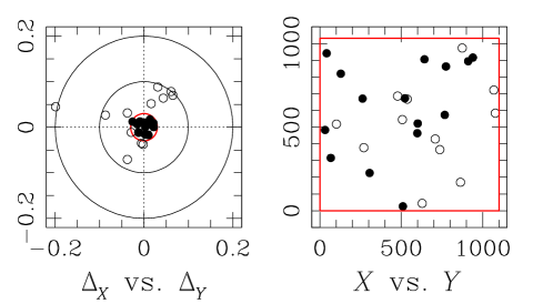
Figure 1: (Left:) Consistency in positions —in units of WFC3/IR pixels— of the sources in common between the Gaia DR2 and our HST reference frame. The concentric circles indicate displacements at 0.03, 0.1 and 0.2 pixels. The sources with positions consistent to better than 0.03 pixels (filled symbols) are used to define the astrometric reference frame (see text). (Right:) With the same symbols, the spatial distribution of these sources in the observational plane $(X,Y)$.

Table 2: Adopted coefficients to transform the observed coordinates $(X,Y)_{2013.1}$ into the tangent plane $(\xi,\eta)_{2013.1}$ linked to Gaia DR2 equatorial coordinates $(\alpha,\delta)_{2013.1}$.

$\mathcal{A}$	$(0.2876330\pm 0.0025)E-04$
$\mathcal{B}$	$(0.1738241\pm 0.0025)E-04$
$\mathcal{C}$	$(0.1739133\pm 0.0025)E-04$
$\mathcal{D}$	$(-0.2875556\pm 0.0025)E-04$
$X_{0}$	$570.631\pm 0.004$
$Y_{0}$	$564.770\pm 0.004$
$\alpha_{0}$	$235.465250$ (defined)
$\delta_{0}$	$-22.840275$ (defined)

The plate-scale derived from Gaia DR2 of our reference frame $(X,Y)_{2013.1}$ is $\sqrt{|{\mathcal{A}\mathcal{D}-\mathcal{B}\mathcal{C}}|}=\sqrt{|\Delta|}=120.984$ mas, in agreement with previous WFC3/IR determinations.

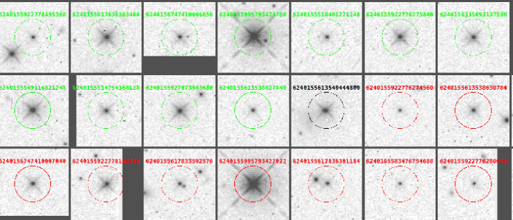
Figure 2: We extracted from the stack in filter F127M, stamps of 100$\times$100 WFC3/IR pixels ($\sim$12^′′$\times$12^′′) centered on the 27 sources in common between the Gaia DR2 catalog and our HST reference frame. Circles with radius of $3^{\prime\prime}$ and labels with the Identifier: Gaia DR2 are given. From left-to-right and top-to-bottom sources are sorted for consistency in positions $\varrho$ (see Table 3). The best stars, the astrometric references, used to compute the transformation in Table 2, are labeled in green. In black, source Gaia DR2 #6240155613540444800 with a significant parallax, and in red stars with displacements between 0.03 and 0.1 pixels (3.6-12 mas). In magenta the worst source, at more than 0.2 pixels (or 24 mas). [See Sect. 3.8.]

3.5 A closer look at the Gaia DR2 sources

More than a third of the sources in common between HST and Gaia DR2 (12/27) have much larger residuals than the others. Under suggestion of our referee, here we investigate and discuss in details possible reasons for this.

The very first step is to have a visual inspection of the astronomical scene and search for possible sources compromised by: crowding, blends, multiple hits of cosmic-rays/bad-pixels, diffraction spikes, and artifacts in general. For this purpose, we use the stack (which will be later described in Sect. 3.8) obtained for images in filter F127M (Fig. 2). We notice that some of the sources with poor positional-consistency (circled in red) have relatively bright sources closer than 3^′′, but we ruled this out as a possible reason, as sources with the best agreement have similar or even worse neighbors. Similarly, being close to the boundary of images does not seem to be a problem, as three sources appear closer than 6^′′ to image boundaries, both in cases of stars labeled in green and in red. Also, sources in red and green seem to have similar ranges of brightness.

The spatial distribution of sources in the right-panel of Fig. 1 seems to suggest that no significant bias of the best vs. worst sources is evident in the plane $(X,Y)$; particularly in the region around the target, at $\sim$(500,500). However, given the small number of sources in the field sufficiently-bright to be detected by Gaia, this is not the ideal case for such a study.

Obviously, the large number of sources with relatively large residuals (open symbols in the right-panel of Fig. 1) are not necessarily due to problems in the Gaia DR2 sources, but could be in our own measurements in the HST images; or in both.

We therefore look at the consistency parameters obtained for sources in the HST reference frame $(X,Y)_{2013.1}$ defined in Sect. 3.2. We look at the trends in the r.m.s. of $X$, $Y$, $M_{\rm F125W}^{instr.}$ (the instrumental magnitude in F125W), and $Q$ (the PSF-quality-fit, as defined in Anderson et al. 2008), as function of magnitude. We found that the brightest star in the field, Gaia DR2 #6240155995793427072, has a much larger r.m.s. in the $X$-position measured within the first epoch (0.148 pixels) compared to the r.m.s. of similar magnitude objects (for example, the second brightest source in the field has an r.m.s. of 0.005 pixels). This explains the rejection of Gaia DR2 #6240155995793427072 from the sample of astrometric reference. We also noted a significantly larger photometric variability of the rejected source Gaia DR2 #6240155613538632576 ($\sim$0.055 mag) compared to that of sources at similar magnitude ($\sim$0.01 mag), which might potentially indicate it to be an unresolved binary.

The next step is to consider astrometric and photometric parameters in the Gaia DR2 catalog. We inspected for all objects the quality indicators available in Gaia DR2. We immediately spot two objects with no proper motions at all. These are Gaia DR2 #6240155617836301184 and the one with the worst positional consistency, i.e., Gaia DR2 #6240155995790716928 (in magenta in Fig. 2). Evidently, the positions for these objects were not corrected in Eq. 5, and their large displacements might just reflect their unknown pms. We also note that Gaia DR2 #6240155613540444800 was rejected as the only source with a significant parallax greater than 3 mas. Of the remaining 9 objects with poor consistency in position in Fig. 1 (larger than 0.03 pixels, or 3.6 mas) we note that only 4 sources passed the tests for well-measured objects in the Gaia DR2 catalog as defined in Eqs. (C.1) and (C.2) by Lindegren et al. (2018). These are Gaia DR2  #6240155613538630784, #6240156747410007040, #6240155583476754688, and #6240155922776280064, with $G$-magnitudes of about 18.8, 19.5, 20.5, and 20.1, respectively. The expected errors for objects in this magnitude interval are about 2 mas (Lindegren et al. 2018), therefore, the observed positional residuals of Gaia DR2 vs. HST (between 3.6 and 12 mas) indicate that these four sources could be reasonably well measured —given their faintness. They were rejected simply because the sum of their random errors (HST$\sim$4 mas and Gaia DR2$\sim$2 mas) are not consistent ($\sim$4.5 mas) with our arbitrary tight cut at 0.03 pixels (3.6 mas).

In Table 3 we list all the relevant HST and Gaia DR2 parameters for the 27 objects in common. The first 14 are the ones defining the astrometric references, the $15^{\rm th}$ is the one rejected for sizable parallax, the next 11 are the ones with poor positional consistency, and at last, the one with the worst consistency ($>$0.2 pixels). In the first column we give the Identifier: Gaia DR2. Next column give the parameters from HST data: $(X,Y)$-positions, instrumental magnitude, and $Q$. Then we give the consistency in positions $\varrho$ in units of WFC3/IR milli-pixels. The next columns give the Gaia magnitudes $G$, proper motions in mas yr^-1, and parallaxes in mas. The last column gives the most relevant Gaia DR2 parameters for the present work. These are: the visibility_periods_used ($v$), the astrometric_n_bad_obs_al ($b$), and the quantities U and G defined in Eqs. (C.1) and (C.2) by Lindegren et al. (2018).

Table 3: The 27 Gaia DR2 sources in common with our HST master frame. Columns give: Identifier: Gaia DR2, $(X,Y)$-positions in WFC3/IR-pixels, HST-instrumental magnitude, the consistency in positions $\varrho$ in WFC3/IR milli-pixels, the Gaia magnitude $G$, proper motions in mas yr^-1, parallaxes in mas, and four of the most significant Gaia DR2 parameters for the present work. The visibility periods used $v$, the number of bad astrometric observations $b$, and the quantities U and G defined in Eqs. (C.1) and (C.2) by Lindegren et al. (2018). The first 14 objects are those used to define the astrometric reference, and have all $\varrho<23.3$ milli-pixel ($\sim$2.8 mas).

Identifier: Gaia DR2	$(X,Y,M_{\rm F125W}^{\textit{instr.}})$	$\varrho$	$G$	($\mu_{\alpha^{*}}\pm\sigma_{\mu_{\alpha^{*}}}$,$\mu_{\delta}\pm\sigma_{\mu_{\delta}}$,$\pi\pm\sigma_{\pi}$)	($v$,$b$,U,G)
6240155617832556544	(0522.088,673.142,$-$7.4134)	2.9	19.525	($-$8.202$\pm$1.126,$-$6.820$\pm$0.802,$-$0.045$\pm$0.620)	(10,2,1,1)
6240155922778495360	(0939.610,917.019,$-$6.8337)	10.5	19.812	($-$3.942$\pm$1.127,$-$2.834$\pm$0.753,$-$0.042$\pm$0.648)	(10,1,1,1)
6240155617836303488	(0600.795,522.307,$-$9.3597)	11.7	17.983	($-$10.407$\pm$0.323,$-$1.714$\pm$0.221,$+$0.639$\pm$0.188)	(10,0,1,1)
6240156747410006656	(0509.842,026.488,$-$7.6669)	15.3	19.307	($-$8.658$\pm$0.949,$-$2.836$\pm$0.821,$+$1.048$\pm$0.500)	(09,1,1,1)
6240155995793424768	(0766.966,573.666,$-$12.0318)	15.6	14.418	($+$11.261$\pm$0.066,$-$12.398$\pm$0.047,$+$0.975$\pm$0.037)	(10,1,1,1)
6240155510461221248	(0128.497,820.398,$-$6.8964)	16.4	20.738	($+$4.171$\pm$3.918,$-$11.174$\pm$2.764,$-$0.233$\pm$1.700)	(09,0,0,0)
6240155922776275840	(0774.182,863.455,$-$8.8226)	16.4	17.811	($+$1.576$\pm$0.295,$-$4.212$\pm$0.205,$+$0.058$\pm$0.170)	(10,0,1,1)
6240156335093137536	(0066.905,316.118,$-$8.3823)	16.6	18.126	($-$11.804$\pm$0.365,$-$7.996$\pm$0.249,$-$0.007$\pm$0.206)	(10,1,1,1)
6240155579178890624	(0031.905,483.388,$-$6.8282)	17.2	19.720	($+$2.040$\pm$1.140,$-$8.564$\pm$0.774,$+$0.158$\pm$0.650)	(10,0,1,0)
6240156369452880000	(0305.537,226.296,$-$7.6479)	18.8	18.914	($-$3.309$\pm$0.612,$+$0.946$\pm$0.411,$-$0.124$\pm$0.361)	(10,0,1,1)
6240155549116821248	(0642.303,906.672,$-$9.6141)	20.1	17.196	($-$4.379$\pm$0.221,$-$7.765$\pm$0.147,$+$0.655$\pm$0.121)	(10,0,1,1)
6240155514754368128	(0041.535,942.644,$-$7.9155)	21.9	20.537	($-$21.354$\pm$2.412,$-$0.103$\pm$1.657,$+$1.602$\pm$1.139)	(09,0,1,0)
6240155927073943680	(0910.703,895.041,$-$9.2091)	21.9	17.326	($-$10.000$\pm$0.243,$+$3.948$\pm$0.170,$+$0.217$\pm$0.135)	(10,0,1,1)
6240155613538627840	(0262.163,671.320,$-$7.0115)	23.2	20.117	($-$1.775$\pm$1.412,$-$10.251$\pm$0.950,$-$0.762$\pm$0.801)	(10,0,1,1)
6240155613540444800	(0598.187,464.043,$-$9.0561)	28.5	19.354	($-$37.833$\pm$0.889,$-$25.853$\pm$0.610,$+$3.857$\pm$0.606)	(10,0,1,1)
6240155922776274560	(0874.306,974.415,$-$6.1297)	30.8	20.614	($+$2.012$\pm$2.491,$-$6.391$\pm$1.710,$+$0.427$\pm$1.166)	(09,0,1,0)
6240155613538630784	(0477.394,686.589,$-$7.7311)	35.6	18.839	($-$3.394$\pm$0.705,$-$4.478$\pm$0.623,$+$0.512$\pm$0.381)	(09,0,1,1)
6240155613538632576	(0269.716,377.640,$-$6.3762)	37.7	20.137	($-$6.979$\pm$1.499,$-$5.074$\pm$1.025,$-$0.398$\pm$0.869)	(10,1,1,0)
6240156747410102144	(0863.329,170.568,$-$7.9744)	48.8	20.194	($-$16.071$\pm$2.526,$-$1.265$\pm$1.739,$+$2.181$\pm$0.961)	(07,3,1,1)
6240156747410007040	(0628.193,044.235,$-$7.8694)	54.2	19.479	($-$0.796$\pm$0.899,$-$11.031$\pm$0.600,$+$0.820$\pm$0.498)	(10,0,1,1)
6240155922778106880	(1077.511,584.057,$-$8.4938)	77.3	19.536	($-$5.770$\pm$1.063,$-$6.684$\pm$0.727,$+$1.444$\pm$0.621)	(10,3,0,0)
6240155617833592576	(0506.614,545.481,$-$7.0274)	80.0	20.525	($-$0.175$\pm$2.270,$-$4.630$\pm$1.558,$+$1.224$\pm$1.104)	(09,0,1,0)
6240155995793427072	(0736.691,366.113,$-$12.5981)	90.7	14.411	($-$13.740$\pm$0.072,$+$4.197$\pm$0.048,$+$0.184$\pm$0.041)	(10,0,1,1)
6240155617836301184	(0536.728,667.953,$-$7.0182)	93.8	21.160	($+$0.000$\pm$0.000,$+$0.000$\pm$0.000,$+$0.000$\pm$0.000)	(06,0,1,0)
6240155583476754688	(0101.508,518.783,$-$6.0182)	95.7	20.546	($-$9.212$\pm$2.330,$-$1.858$\pm$1.687,$+$1.427$\pm$1.558)	(09,0,1,1)
6240155922776280064	(1067.981,722.722,$-$6.3521)	99.4	20.089	($-$4.689$\pm$1.359,$-$0.037$\pm$0.935,$-$1.092$\pm$0.797)	(10,0,1,1)
6240155995790716928	(0708.427,429.764,$-$7.1248)	204.1	20.927	($+$0.000$\pm$0.000,$+$0.000$\pm$0.000,$+$0.000$\pm$0.000)	(06,0,1,0)

3.6 Geometric-distortion solution of WFC3/IR

In this section we investigate $(i)$ at what level the imperfections in the adopted WFC3/IR distortion solution could affect our results, and $(ii)$ whether Gaia DR2 could actually be used to improve the current geometric distortion solutions of HST cameras.

3.6.1 Effects of WFC3/IR distortion uncertainties

First of all, even from frame to frame —consecutively taken— the simple velocity aberration (Cox & Gilliland 2003) can cause sizable changes in the plate-scale. Good telemetry (or accurate modelling of the HST orbits) can fix these effects (e.g., Fig. 9 in Bellini, Anderson & Bedin 2011). Note that this is merely a scale factor induced by the motion of the telescope in special relativity and has nothing to do with the distortion of the camera itself, but still is a sizable effect that needs to be taken carefully into account when applying the geometric distortion solution and dealing with absolute astrometry.

Second, as extensively discussed in Bedin et al. (2014), any adopted geometric distortion correction for any of the HST  cameras is just an average solution. Even after correction for velocity aberration, there are always sizable changes and these are mainly induced by focus variations, the so called breathing of the telescope tube, which are the result of the different incidence of the light from the Sun. Detailed models of these changes in the geometric distortion with the focal length are still not developed, so far there are only early attempts of modelling the changes in the PSFs as function of focal length (Anderson & Bedin 2017).

Third, it is known that linear terms of the ACS/WFC distortion solution have been changing slowly over time (Anderson & Rothstein 2007; Ubeda, Kozhurina-Platais & Bedin 2013), the reasons of these effects are still not clear, probably the result of a slow out gas of metal that shrink structures and cause these long-term changes. However, in the case of WFC3/IR, a recent study by McKay & Kozhurina-Platais et al. (2018) showed that the linear terms of the geometric distortion is stable at the level of 13 mas over an eight years time span.

The best available geometric distortion solutions for HST cameras are composed by the sum of a polynomial and of an empirical look-up table (e.g., Anderson & King 2000, 2003, 2006 for descriptions in great details). Thankfully, all of the three effects, i.e., velocity aberration, breathing, and shrinking, just described, cause detectable changes only in the linear part of the geometric distortion, while the non-linear part of the distortion seems to remain unchanged within the uncertainties (at the $\sim$ 1 mas level).

The beauty of our approach is that the six-parameters linear transformation derived in Sect. 3.2 that calibrates our HST master frame to the absolute reference frame of Gaia DR2 (Table 2), naturally absorbs all of these three effects, fixing the values of: absolute scale, rotation, shifts and the two skews terms. In other words, the linear terms of the geometric distortion can change by a lot (even by few dozen of mas), but as long as we use the most-general linear transformation (a 6-parameters) to calibrate our $(X,Y)$ reference system to Gaia DR2 absolute astrometric reference frame, all of these effects do not prevent us from achieving accuracies limited just by our positional accuracy ($\sim$1 mas) and by the stability of the non-linear part of the adopted geometric distortion solution.

Our adopted WFC3/IR geometric distortion solution was derived by Anderson (2016, pg. 39, Appendix A). Unlike WFC3/UVIS and the ACS channels, which have separate solutions for each filter, there is only one solution that works for all WFC3/IR filters. So far variation with filters were not explored, but any variation is likely less than $\sim$0.01 pixel (i.e., $\sim$1.2 mas, cfr. Anderson 2016). Precisions of $\sim$1 mas (differential astrometry) with WFC3/IR are now routinely reached (e.g., Anderson 2016, Bellini et al. 2017, 2018, Libralato et al. 2018), and the Gaia DR2 catalog now makes it possible to transform those precisions into absolute-astrometric accuracies, for the reasons just outlined. This is demonstrated by the displacements observed in Fig. 1 (and in a similar figure presented later in Sect. 3.7) of this work.

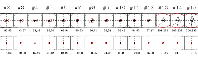
Figure 3: The sources in common between the Gaia DR2 catalog and those measured (and corrected for distortion) on a given image define a six-parameters linear transformation. With this transformation we can predict the positions of Gaia DR2 sources in that image, and visa-versa. Panels in this figure all have the same scale ($-$0.5,+0.5 WFC3/IR pixels in both $X$ and $Y$) and show the displacements between the observed and the predicted Gaia DR2 positions based on the transformations obtained for each of the 16 images. On the –Top Panels– however, positions of Gaia DR2 sources were not corrected for their individual tabulated Gaia DR2 proper-motions. Above each panel the #id to which each image refers is indicated (following notation in first column of Table 1). Note that #1-4 were taken at 2013.1, #5-12 at 2013.3, and #13-16 at 2018.1. Red ellipses indicate the 3$\sigma$ of the distribution along the X and Y axes, and their 1$\sigma_{X,Y}$ values in WFC3/IR milli-pixels are indicated below of each panel. On the –Bottom Panels– positions of Gaia DR2 sources were corrected for their individual proper-motions. It is clear that in the bottom panels the dispersion of observed vs. Gaia DR2 positions are much tighter (better than $\sim$3 mas) than in the top panels, and also consistent across all 16 images (with a slight broadening for images with the shortest exposure times, particularly in the F105W filter).

In summary, as the non-linear part of the adopted geometric distortion solution is as accurate as our positional accuracy for best measured stars, i.e., $\sim$1 mas, we do not expect residuals in the distortion to be a significant source of uncertainty in deriving the astrometric parameters for W1541$-$2250. This target is a source more than 6 magnitudes fainter than best measured stars in the field, having an estimated positional precision between 5 and 12 mas in individual images (depending on filter/exposure-time). Furthermore, any of such distortion residual would be suppressed by averaging over multiple dithered observations within each of the individual epochs.

3.6.2 Can HST distortion be improved with Gaia DR2?

For a well-exposed point-source the positional accuracy on images from HST’ cameras is $\sim$1 mas (at best 0.32 mas for WFC3/UVIS, Bellini et al. 2011), and the non-linear part of the geometric distortion solution is proven to be at least that good.

So, even with an infinitely accurate geometric distortion solution for HST cameras, a given target would require multiple observations to improve the astrometry at the sub-mas level, given the limit on the accuracy set by random noise (i.e., the possible exposure time or saturation level) in individual images. This drastically reduces the number of applications where a sub-mas level accuracy for the geometric distortion solution would be worth and useful. For example, the comparison with Gaia DR2 in the case of a group of point sources within an HST field of view (such as stars in a star cluster) can statistically highlight sub-mas trends in the geometric distortion solution. In this regard, the recent work by Kozhurina-Platais et al. (2018) discuss the potential importance of such improvements, especially in the low-order components of the distortions down to the level of 0.5 mas or better.

However, for high-order components (i.e., on small spatial scales) there is a fundamental limitation in using Gaia astrometric catalogs to improve HST’ camera distortion solutions, and this is the spatial density of Gaia sources. The Gaia DR2 catalog has an ’all-sky’-average density of $\sim$10 sources per arcmin square, and this essentially is set by its magnitude limits. For example, effects such as the WFPC2 34^th-raw feature discovered and fixed by Anderson & King (1999), or the WFC3/UVIS lithographic signatures found by Kozhurina-Platais et al. (2010) and later characterized in Bellini et at. (2011) would have been very hard to calibrate by using just Gaia DR2 sources.

One might think of comparing Gaia DR2 sources with multiple fields and multiple epochs or even with the entire archive of HST observations to characterize such effects or any high-order components of the geometric distortion in general; however not using the same sources with a suitable density and within the same epochs, would exponentially complicate the calibration, which also, might well be variable in time at the sub-mas level. Self calibration of HST (e.g., Anderson & King 1999, 2000, 2003, 2006, Bellini et al. 2011) and local transformations in dense fields (e.g., Bedin et al. 2003, 2014, Anderson & van der Marel 2009, Bellini et al. 2017, 2018) would offer a much easier way to calibrate and characterize such effects and high-order components of the geometric distortion in general, than using sources in common with Gaia.

Finally, we want to note that at the sub-mas level —even ignoring chromatic effects— there is always an interplay between the adopted geometric distortion and the exact shape of the PSFs, as a slightly different PSFs cause slightly different centroids offsets (which depend on the adopted PSF-centroid normalization), which result in slight changes in the distortion. In other words, at sub-mas level the adopted PSFs model and the adopted geometric distortion solution become more and more an indissoluble pair.

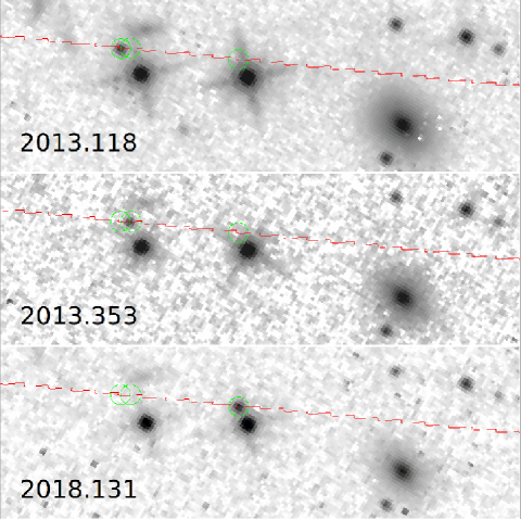
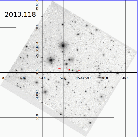
Figure 4: (Left:) Zoom-in of the HST field surrounding W1541$-$2250, as collected in the three epochs analyzed in this work. This small region has a size of $\sim 20^{\prime\prime}\times 6.5^{\prime\prime}$. Green circles indicate the BD positions at the three epochs. A red line show our astrometric solution of the motions for this object in years from 1990 to 2030. (Right:) The entire field of view is about 2.2^′$\times$2.2^′ and this is the stack of four WFC3/IR/F125W images collected in first epoch, where the BD has highest signal. The grid and labels are in equatorial coordinates.

3.7 Link all epochs to Gaia DR2

Similarly to what was done for the reference epoch, we can use Eq. 5 to have pms-corrected position of Gaia DR2 sources at all the different epochs of images in Table 1. Again, Eq. 3 is used to have the coordinates in the tangential plane $(\xi,\eta)_{epoch}$. However, this time we will not have to re-derive the coefficients of the linear transformation from Gaia $(\alpha,\delta)_{epoch}$ to $(X,Y)_{2013.1}$, as those were determined in Sect. 3.4. We now have the Gaia DR2 positions of individual sources, corrected for their peculiar motions, at any given epoch, and in the reference system of $(X,Y)_{2013.1}$. So we can now compute instead the coefficients of the transformations from these Gaia pms-corrected positions at any given epoch registered to $(X,Y)_{2013}$, and the observed positions of sources in each image $(x^{\rm cor},y^{\rm cor})$. The peculiar motions of the sources will not affect the transformations, which will now only be affected by the positioning random errors in the given HST image and by errors (in both positions and pms) in the Gaia DR2 catalog.

To better expose the gain of this procedure, in Fig. 3 we show for each given image the consistency of positions measured $(x^{\rm cor},y^{\rm cor})$ with respect to the positions of Gaia DR2. In the top panels, the Gaia DR2 positions are fixed as tabulated for epoch 2015.5. In the bottom panels, we take advantage of Gaia DR2 pms to correct the positions of sources for their peculiar motions at the exact epoch of the observation. Accounting for peculiar motions of sources reduce the dispersion from the 1-$\sigma$ of 300-50 milli-pixels (37-6 mas, in top panels) to a rather uniform 15-25 milli-pixels (1.8-3 mas).

Once the transformations determined using sources in common between Gaia DR2 and $(x^{\rm cor},y^{\rm cor})$ are known, the positions of all sources in all images (i.e., including those not present in the Gaia DR2 catalog, such as W1541$-$2250) can be transformed in the Gaia system, and their displacements used to measure their astrometric parameters, now with negligible errors in the transformations.

3.8 Stack images

The transformations from the coordinates of each image into the coordinates of the reference frame $(X,Y)_{2013.1}$ enable us to create stacked images for each epoch. Stacked images offer a representation of the astronomical scene that can be used to independently check sources in each image. In left panels of Fig. 4 we show a $\sim 20^{\prime\prime}\times 6.5^{\prime\prime}$ zoom around W1541$-$2250 –from top to bottom– for the stack from first epoch in F125W, second epoch in F125W, and the third in F127M. In the right panel we show the entire field of view as in first epoch, the one with the highest signal for the BD. Our stacked images are saved in fits format, and their headers include (as World Coordinate System keywords) the absolute astrometric solution of Table 2. In the electronic material provided with this work, we release these three stacked images, one per epoch all with our astrometric solution in their header. Note that the $(X,Y)$ coordinates in Table 3 are in the same pixel-coordinate system as these stacks.

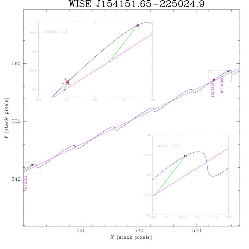
Figure 5: Comparison of our astrometric solution (in blue) with the individual observed data points (red crosses) for W1541$-$2250 in the observational plane $(X,Y)_{2013.1}$. The three major epochs are indicated by labels, and two insets indicated by the gray boxes, with (1) and (2), show a more meaningful zoom-in of the data points. To better highlight the parallax component of the motion a line in magenta indicates an object with the same motion but at infinite distance. Green lines show the parallax contributions at each epoch, and red segment connects the individual data points with their expected position according to the best fit.

4 Determination of Positions, Proper Motions and Parallax

From the observed 16 $\times$ 2D-data points we would like to derive the five astrometric parameters of W1541$-$2250: its positions $(X,Y)$, its motions $(\mu_{X},\mu_{Y})$, and most importantly the parallax ($\pi$). We will describe in the following the procedure followed to fit these five parameters.

By virtue of the principle that any transformation of the observational data degrades them, while numerical models do not, we perform this numerical fitting process directly in the observational plane $(X,Y)_{2013.1}$. To predict the position of W1541$-$2250 we make use of the sophisticated tool by U.S. Naval Observatory, the Naval Observatory Vector Astrometry Software, hereafter NOVAS (in version F3.1, Kaplan et al. 2011), which accounts for many subtle effects, such as the accurate Earth orbit, perturbations of major bodies, nutation of the Moon-Earth system, etc. We are not interested in the absolute astrometric calculations of NOVAS but only in the relative effects. In computing the positions we used an auxiliary star with no motion and zero parallax (i.e., at infinite distance), and finally compute the difference with respect to our target. We then use a Levenberg-Marquardt algorithm (the FORTRAN version lmdif available under MINIPACK, Moré et al.  1980) to find the minimization of five parameters: $X,Y,\mu_{X},\mu_{Y},$ and $\pi$.

Table 4: Astrometric parameters of W1541$-$2250 in the ICRS. Positions are given at three relevant epochs, where the ^ϖ suffix indicates the apparent position with the annual parallax included.

$\alpha_{2000.0}$ [ h m s ]	15:41:52.28891	$\pm$ 5.32 mas
$\delta_{2000.0}$ [ ∘ ′ ′′ ]	$-$22:50:24.74111	$\pm$ 5.74 mas
$\alpha_{2000.0}$ [degrees]	235.46787051	$\pm$ 5.32 mas
$\delta_{2000.0}$ [degrees]	$-$22.84020586	$\pm$ 5.74 mas
$\alpha_{2013.1}^{\varpi}$ [degrees]	235.4643508	$\pm$ 1.0  mas
$\delta_{2013.1}^{\varpi}$ [degrees]	$-$22.84053754	$\pm$ 1.3  mas
$\alpha_{2015.5}$ [degrees]	235.46365494	$\pm$ 2.3  mas
$\delta_{2015.5}$ [degrees]	$-$22.84058569	$\pm$ 1.2  mas
$\alpha_{2015.5}^{\varpi}$ [degrees]	235.46362187	$\pm$ 3.8  mas
$\delta_{2015.5}^{\varpi}$ [degrees]	$-$22.84058063	$\pm$ 1.4  mas
$\mu_{\alpha\cos{\delta}}$ [mas yr-1]	$-$902.62	$\pm$ 0.35
$\mu_{\delta}$ [mas yr-1]	$-$88.26	$\pm$ 0.35
$\pi$ [mas]	168.38	$\pm$ 2.23
$\varpi=\pi+0.2$ [mas]	168.58	$\pm$ 2.23 $\pm$0.4

Our final astrometric solution is given in Table 4 and shown in Fig. 5. To assess the uncertainties of our solution we perform 25 000 simulations where, to the expected positions $(X,Y)$ from our best-fit astrometric solution, we added random errors following Gaussian distributions with dispersion derived from the observed data of W1541$-$2250 for each of the four filter/epoch combinations (i.e., F125W@2013.1, F105W@2013.3, F125W@2013.3, and F127M@2018.1).

Our astrometric parameters agree well with the two best estimates in literature, those by Tinney et al. (2014) and Beichman et al. (2014), and represent a significant improvement. Furthermore, our solution surely does not suffer of any of the usual ground-based atmospheric effects and relies on the homogeneous data, therefore providing an important confirmation.

In addition to Fig. 5 and its insets, in Fig. 6 we show also the parallax ellipse along with HST measurements [proper motion subtracted]. This representation better reveals the sampling of the parallactic motion which, with only three epochs, could be problematic.

We note few things in this figure. First, the parallax ellipse is extremely flattened, as an obvious consequence of the extremely low-latitude ecliptic coordinates for W1541$-$2250, i.e., $(\ell,b)=(\sim 238^{\circ},\sim-3^{\circ})$.

Second, we know that the first (2013.1) and the last epoch (2018.1) were collected almost exactly 5 yrs apart; meaning that they were collected almost exactly at the same phase of the year.

Third, we know also these two epochs to be taken at one of the maxima of the parallax elongation, and indeed, their positions on the parallax ellipse agree with eachother, and with the position of the maximum. These two epochs also have the greatest accuracies (thanks to the filter/exposure-time combination) and have the largest possible time base-line among the epochs. This is a great advantage to derive the astrometric parameters, as these two epochs alone could essentially fix the proper motions of W1541$-$2250 with great accuracy. The determination of the parallax therefore, essentially relies in the second epoch (2013.3), which thankfully was collected at a significantly different phase of the year allowing us to well constrain this astrometric parameter. Unfortunately the second epoch has also the lowest accuracy of the three and therefore ultimately sets the limits in the accuracy of the here derived parallax for W1541$-$2250.

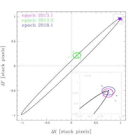
Figure 6: Our solution for the parallax ellipse in the $(X,Y)_{2013.1}$ coordinate system. Individual HST data-points are indicated with star-symbols, which are connected with small segment to their expected position according to our best fit. Smaller ellipses in magenta, green, and blue, indicate the 1-$\sigma_{X,Y}$ of individual data points within the first, second and third epoch, respectively. Note how ellipses are significantly smaller for the first and third epoch (0.025-0.020 and 0.031-0.020 WFC3/IR-pixels, i.e., 3.0-2.4 and 3.8-2.4 mas), compared to the second epoch (0.079-0.056 pixels, i.e., 9.5-6.8 mas). However, second epoch has twice as many images than each of the other two, therefore, as the error on the average $\overline{\sigma}$ scales as $\sim\sigma/\sqrt{n-1}$ (with $n$ equal to the number of images), the net worsening for this epoch is at most a factor 2. An inset in gray, zoom-in at a busy location around the maximum parallax elongation, marked by a gray box.

Table 5: List of works in the Literature providing astrometric parameters for W1541$-$2250.

work	$\mu_{\alpha^{*}}\pm\sigma\mu_{\alpha^{*}}$	$\mu_{\delta}\pm\sigma\mu_{\delta}$	$\pi\pm\sigma_{\pi}$	$d$	source
#. authors (date)	[mas yr-1]	[mas yr-1]	[mas]	[pc]	facilities
1. Cushing et al. (2011)	…	…	…	8.1 (8.1-8.9)	Magellan+WISE
2. Kirkpatrick et al. (2011)	…	…	$351\pm 108$	2.2-4.1	Magellan
3. Kirkpatrick et al. (2012)	…	…	$238$	4.2∗	WISE
4. Dupuy & Kraus (2013)	$-870\pm 130$	$-13\pm 58$	$74\pm 31$	$14^{+10}_{-4}$	Spitzer
5. Marsh et al. (2013)	$-983\pm 111$	$-276\pm 116$	$-21\pm 94$	$>6.0$	WISE+Spitzer+Magellan+CTIO
6. Tinney et al. (2014)	$-894.7\pm 4.2$	$-87.7\pm 4.7$	$175.1\pm 4.4$	…	Magellan
7. Beichman et al. (2014)	$-857\pm 12$	$-87\pm 13$	$176\pm 9$	$5.7\pm 0.3$	Keck+Spitzer+HST
8. Martin et al. (2018)†	$-895.05\pm 4.68$	$-94.73\pm 4.66$	$167.05\pm 4.19$	$5.99^{+0.154}_{-0.147}$	Spitzer
9. this work	$-902.62\pm 0.35$	$-88.26\pm 0.35$	$169\pm 2$	$5.9\pm 0.1$	HST+Gaia
∗ spectro-photometric distance, to which they refer as ’adopted distance’
† while our article was still under review

4.1 The Absolute Parallax

The transformations of coordinates described in previous sections were computed with respect to Gaia DR2 sources, which are not at infinite distance. Therefore the relative parallax we have derived in Sect. 4 (which we indicate with $\pi$) of W1541$-$2250 is with respect to the most distant objects in the field and therefore $\pi$ is only a lower limit on the absolute parallax (which we indicate with $\varpi$). Gaia DR2 catalog potentially gives the possibility to correct the positions of sources –at any give epoch– not only for individual pms, but also for the amplitude of the parallax at any given phase of the year. However, given the accuracies in this work, it will be sufficient to correct for the clipped mean parallax of the sources used to compute the parameter of the transformation given in Table 4. Twelve of the 15 stars used to compute the transformation have a parallax consistent with zero, and only two have a significant parallax of about $\sim$1 mas. Only one of the reference sources, Gaia DR2 #6240155613540444800, had a significant large parallax of 3.857$\pm$0.606 mas, and was rejected. The computed average parallax of the remaining 14 sources is 0.3$\pm$0.2 mas, while their median is 0.16 mas with a semi-interquartile of 0.35 mas. Given the uncertainties, we adopt 0.2$\pm$0.4 mas as correction from relative to absolute parallax. In Table 4 we also give the value derived for $\varpi$ employing this correction. The $\varpi$ and uncertainties translate in an estimated distance for W1541$-$2250 of $d=5.9\pm 0.1$ pc. The uncertainty in the estimated relative parallax of W1541$-$2250 amounts to $\sim$2.3 mas, making the correction from relative to absolute an unnecessary calculation in this case.

Future applications of this method to cases that would actually need higher accuracy will require to calculate —for each of the reference sources— the exact positions corrected for the parallax (in addition to corrections for pms), before computing the coordinate transformations.

5 Conclusions

In this paper we employed three archival and proprietary HST  epochs to derive an independent and robust estimate of the astrometric parameters of WISE J154151.65$-$225024.9, one of the only 23 confirmed Y BDs (as September 14^th 2018), and the fifth closest.

We have developed a procedure that makes use of the Gaia DR2 catalog of positions, proper motions and parallaxes, to minimize the errors in the transformations that used to limit traditional relative imaging-astrometry with narrow-field cameras. We gave here an extensive explanation and many details of our procedure, with the intent of using it in future articles that will refer to the present work. Indeed, future papers will be focused on the science (mainly based on the derived multi-band photometry) and will minimize description of the technicalities to derive the distances.

The derived astrometric parameters for W1541$-$2250 are summarized in Table 4 and represent sizable improvements over recent determinations in the literature which are summarized in Table 5. Worth to notice that the here derived relative parallax of $\pi=168.38\pm 2.23$ mas (i.e., with an accuracy better than 1.3%) is well in agreement (at the 1.5 $\sigma$-level) with the best available (and completely independent) estimate by Tinney et al. (2014) ($\pi=175.1\pm 4.4$ mas), which was based on ground-based observations. Ground-based observations are generally afflicted by atmospheric effects and gravity-induced flexes in the telescope/camera structures that generate systematic errors often difficult to correct, particularly when assessing the astrometry of faint and red sources (much redder than reference field stars). Therefore, the homogeneous space-based HST  data provide an important update and confirmation of those previous estimates for the W1541$-$2250 parallax.

Applying a Gaia DR2 correction from relative ($\pi$) to absolute ($\varpi$) parallax we found $\varpi$=169$\pm$2 mas, corresponding to a distance of 5.9$\pm$0.1 pc for W1541$-$2250, marginally larger than previously estimated, but in agreement with the most recent determination by Martin et al. (2018, accepted paper in press, private communication) based on Spitzer data.

References

- [] Anderson J. & King I. R., 1999, PASP, 111, 1095
- [] Anderson J., King I. R., 2000, PASP, 112, 1360
- [] Anderson J., King I. R., 2003, PASP, 115, 113
- [] Anderson J. & King I. R., 2006, Instrument Science Report ACS 2006-01, STScI, Baltimore
- [] Anderson, J. et al. 2008, AJ, 135, 2055
- [] Anderson J., van der Marel R. P., 2010, ApJ, 710, 1032
- [] Anderson, J. & Bedin L. R. 2017, MNRAS, 470, 948
- [] Anderson J., Rothstein S. M, 2007, Instrument Science Report ACS 2007-08, STScI, Baltimore
- [] Anderson J. 2016, Instrument Science Report WFC3 2016-12, STScI, Baltimore
- [] Bedin, L. R. et al. 2003, AJ, 126, 247
- [] Bedin, L. R., Pourbaix, D., Apai, D., et al. 2017, MNRAS, 470, 1140-1155
- [] Bedin, L. R. et al. 2014, MNRAS, 439, 354
- [] Bellini, A., Anderson, J. & Bedin, L. R. 2011, PASP, 123, 622
- [] Bellini, A. et al. 2017, ApJ, 842, 6
- [] Bellini, A. et al. 2018, ApJ, 853, 86
- [] Libralato, M. et al. 2018, ApJ, 854, 45
- [] Beichman, C., Gelino, C. R., Kirkpatrick, J. D., et al. 2014, ApJ, 783, 68
- [] Cox C., Gilliland R. L., 2003, in Arribas S., Koekemoer A., Whitmore B., eds, The 2002 HST Calibration Workshop: Hubble after the Installation of the ACS and the NICMOS Cooling System. STScI, Baltimore, p. 58
- [] Cushing, M. C., Kirkpatrick, J. D., Gelino, C. R., et al. 2011, ApJ, 743, 50
- [] Dressel L., 2017. Wide Field Camera 3 Instrument Handbook, Version 9.0., STScI, Baltimore
- [] Dupuy, T. J., & Kraus, A. L. 2013, Sci, 341, 1492
- [] Fontanive, C., Biller, B., Bonavita, M., Allers, K, 2018, MNRAS, 473, 2702
- [] Gaia Collaboration, 2016, A&A, 595, id.A1
- [] Gaia Collaboration, 2018, A&A in press, arXiv: 1303.5345
- [] Kaplan, G, Bartlett, J., Monet, A., Bangert, J. & Puatua, W., 2011, User’s Guide to NOVAS Version F3.1, (Washington, DC: USNO).
- [] Kirkpatrick, J. D., Cushing, M. C., Gelino, C. R., et al. 2011, ApJS, 197, 19
- [] Kirkpatrick, J. D., Gelino, C. R., Cushing, M. C., et al. 2012, ApJ, 753, 156
- [] Kozhurina-Platais, V. et al. 2018, Instrument Science Report WFC3 2018-01, STScI, Baltimore
- [] Kozhurina-Platais, V., et al., 2010, in “2010 HST Calibration Workshop”, eds Deustua, S., Oliveira, C., (Baltimore:STScI)
- [] Lindegren, L. et al. 2018, A&A, 616, 2
- [] Martin, E. et al. 2018, arXiv:1809.06479
- [] McKay, M. & Kozhurina-Platais, V. 2018, Instrument Science Report WFC3 2018-09, STScI, Baltimore
- [] Moré, J. J., Garbow, B. S. & Hillstrom, K. E. User Guide for MINPACK-1, Argonne National Laboratory Report ANL-80-74, Argonne, Ill., 1980
- [] Opitz, D., Tinney, C. G., Faherty, J. K., Sweet, S., Gelino, C. R., Kirkpatrick, J. D 2016, ApJ, 819, 17O
- [] Schneider, A. C., Cushing, M. C., Kirkpatrick, J. D., et al. 2015, ApJ, 804, 92
- [] Smart, W. M. on “Textbook on Spherical Astronomy”, First Edition 1931, Edited by Cambridge University Press, Six Edition 1977, tranferred to digital printing 1999, ISBN 0-521-29180-1
- [] Tinney, C. G., Faherty, J. K., Kirkpatrick, J. D., Cushing, M., Morley, C. V., Wright, E. L. 2014, ApJ,796, 39
- [] Ubeda L., Kozhurina-Platais V., Bedin L. R., 2013, Technical Report, ACS/WFC Geometric Distortion: A Time Dependency Study, Baltimore, MD ACS/WFC Geometric Distortion: a Time Dependency Study (ISR 13-03)