Coevolutionary patterns caused by prey selection

Sabrina B. L. Araujo^1,2,∗, Marcelo Eduardo Borges^2,3, Francisco W. von Hartenthal³ , Leonardo R. Jorge^4,5 , Thomas M. Lewinsohn⁴, Paulo R. Guimarães Jr.⁶ and Minus van Baalen⁷

¹Departamento de Física, Universidade Federal do Paraná, 81531-980, Curitiba, Paraná, Brazil.

²Laboratório de Ecologia e Evolução de Interações, Biological Interactions, Universidade Federal do Paraná, P.O. Box 19073, PR 81531-980, Curitiba, Brazil.

³ Pós-Graduação em Ecologia e Conservação, Setor de Ciências Biológicas, Caixa Postal 19031, Curitiba, PR, 81531-990, Brazil.

⁴Departamento de Biologia Animal, Instituto de Biologia, UNICAMP, Campinas, Brazil.

⁵Department of Ecology, Institute of Entomology, Biology Centre, Czech Academy of Sciences, České Budějovice, Czech Republic.

⁶Departamento de Ecologia, Instituto de Biociências, USP, São Paulo, Brazil.

⁷IBENS CNRS UMR8197, ENS, Paris, France.

*Corresponding author: araujosbl@gmail.com

Abstract

Many theoretical models have been formulated to better understand the coevolutionary patterns that emerge from antagonistic interactions. These models usually assume that the attacks by the exploiters are random, so the effect of victim selection by exploiters on coevolutionary patterns remains unexplored. Here we analytically studied the payoff for predators and prey under coevolution assuming that every individual predator can attack only a small number of prey any given time, considering two scenarios: (i) predation occurs at random; (ii) predators select prey according to phenotype matching. We also develop an individual based model to verify the robustness of our analytical prediction. We show that both scenarios result in well known similar coevolutionary patterns if population sizes are sufficiently high: symmetrical coevolutionary branching and symmetrical coevolutionary cycling (Red Queen dynamics). However, for small population sizes, prey selection can cause unexpected coevolutionary patterns. One is the breaking of symmetry of the coevolutionary pattern, where the phenotypes evolve towards one of two evolutionarily stable patterns. As population size increases, the phenotypes oscillate between these two values in a novel form of Red Queen dynamics, the episodic reversal between the two stable patterns. Thus, prey selection causes prey phenotypes to evolve towards more extreme values, which reduces the fitness of both predators and prey, increasing the likelihood of extinction.

Keywords

coevolution, predator-prey, matching phenotype, predator strategy, victims preference, prey selection

1 Introduction

Antagonistic interactions are an ubiquitous phenomenon in nature, in which one species gains resources at the expense of another. Victim-exploiter relationships encompass a range of interspecific interaction modes such as plant-herbivore, prey-predator and host-pathogen interactions. These interactions can exert reciprocal selective pressures resulting in genetic changes in populations; what is defined as coevolution (Janzen 1980). In the last decades, many theories have been formulated to explain and better understand how interacting species affect the evolution of others (e.g. Thompson (2005) and Abrams (2000)).

One of the most influential hypotheses in coevolution is the Red Queen Dynamics (van Valen 1973), which proposes that species must constantly adapt as a response to the unceasing adaptations of the organisms with which it interacts. As the fitness of the exploited species is reduced, selection will favor those organisms with a better capability of defending themselves or evading exploiters, whereas exploiters will be selected to evolve countermeasures (Hochberg and van Baalen 1998). Many empirical examples and systems that attain such dynamics are already well known and studied, as between birds and avian brood parasites (Avilés et al. 2006; Martín-Gálvez et al. 2006; Refsnider and Janzen 2010; Noh et al. 2018) and between herbivorous insects and their host plants (Ehrlich and Raven 1964; Chew 1977; Nylin et al. 2005; Merrill et al. 2013).

Two frequent ingredients present in coevolutionary antagonistic models are stabilizing and interaction selections. Stabilizing selection favors an optimum phenotype that the population would evolve towards in absence of any other selective pressure. The interaction selection depends on both victim and exploiter phenotypes and, once the interaction is antagonistic, it does not favor the convergence between victim and exploiter phenotypes. Although the intensity of the interaction selection is able to limit the range of phenotypes that an exploiter can succeed in attacking, it does not limit the phenotype range that an exploiter will try to attack. It means that the individual behavior in searching victims is not under selection when no other pressure aside from stabilizing and interaction selections is considered (Matsuda 1985). Some models on optimal foraging strategies have already highlighted the possibility of prey selection (victim choice) may have important consequences on the population dynamics (Stephens and Krebs 1986; Berec 2000), however they do not incorporate evolutionary dynamics. On the other hand, most models for predator-prey coevolution do not impose any priority on predators’ attacks, which imply that they attack at random in their predation neighborhood (see e.g, Murdoch 1969; May 1974; Hutson 1984; Matsuda 1985; Gleeson and Wilson 1986; Gendron 1987; Fryxell and Lundberg 1994; Abrams and Kawecki 1999; van Baalen et al. 2001). An exploiter can increase its fitness if it can choose the victim that maximizes its chances of success instead of interacting randomly. A classical empirical example is brood parasites, known to coevolve with their hosts (Rothstein 1990). Brood parasites can choose to parasitize a host when their eggs match their host’s egg colour (Resetarits 1996; Avilés et al. 2006; Refsnider and Janzen 2010; Soler et al. 2014). The choice of host has consequences for offspring success and therefore it is subject to strong selection (Resetarits 1996; Refsnider and Janzen 2010). There is also a vast literature on insect oviposition patterns suggesting that host plant preference and selection has a significant role in the coevolutionary history of these species (Chew 1977; Jorge et al. 2014; Nylin et al. 2005; Merrill et al. 2013).

The evolutionary patterns predicted by coevolutionary models are a result of different pressures in which coevolutionary interactions occur (Thompson 2005) Specifically, when the interaction selection is determined by the similarity of the interacting species’ phenotypes - phenotype matching (Brown and Vincent 1992; Berenbaum and Zangerl 1998; Gomulkiewicz et al. 2000; Abrams 2000; Gandon and Michalakis 2002; Nuismer and Thompson 2006; Calcagno et al. 2010; Yoder and Nuismer 2010; Gokhale et al. 2013; Andreazzi et al. 2017) - prey phenotype can evolve to values adjacent to the phenotype predators aim at. When stabilizing selection and non-directional interaction selection are combined and assume a symmetrical shape (e.g., as a Gaussian function), the predicted temporal population phenotype distributions are also symmetrical with respect to the optimum phenotype favored by stabilizing selection, resulting in symmetrical coevolutionary branching (Brown and Vincent 1992; Abrams 2000; Calcagno et al. 2010; Yoder and Nuismer 2010) or symmetrical coevolutionary cycling (Gomulkiewicz et al. 2000; Abrams 2000; Dieckmann et al. 1995). In the former, the population phenotypes evolve towards a set of stable phenotypes symmetrically distributed around the optimum phenotype favored by stabilizing selection while in the latter the phenotypes oscillate around it. On the other hand, when the interaction selection is directional (for example when the outcome of the interaction is determined by phenotype differences among interacting species), prey have a preferential evolution pathway imposed by the interaction (Abrams 2000). As a consequence, the symmetry is broken (this is clearly shown by Yoder and Nuismer (2010)). Even though there are abundant studies modeling co-evolutionary patterns, we still lack in understanding how the individual behavior in victim preference by the exploiters modulates these patterns.

To investigate the effects of prey selection in the coevolutionary dynamics of antagonistic populations, we approach the evolutionary predator-prey system where the individual phenotypes related to the interaction can evolve subject to both interaction (phenotype matching) and stabilizing selections. These selective pressures are assumed to have symmetrical shape, which is expected to promote symmetrical coevolutionary patterns: symmetrical coevolutionary branching and symmetrical coevolutionary cycling. We explore the coevolutionary outcomes in phenotypic evolution considering two scenarios: (i) Predation occurs at random; (ii) predators select which prey to attack among those present in the predator’s ‘attack neighborhood’, according to phenotype matching. We then analyze the individuals’ payoffs and also propose an individual-based model where individual phenotypes are explicitly modeled and predators have a limited predation neighborhood. Both approaches agreed that prey selection can promote an asymmetrical stable pattern. Moreover, simulation outcomes allowed us to assess the robustness of our findings and also its sensitivity under different strengths of interaction selection and carrying capacity.

2 Methods

From now on, we will refer the two trophic level populations as prey and predators, but they can also stand for herbivores and food plants, or for parasites or parasitoids and their hosts.

Consider two finite populations of predators and prey. The phenotype of each individual i in a given generation is represented by a real number, $u_{i}$ ($v_{i}$), where $i$ identifies the individual and $u$ ($v$) the prey (resp. predator) species. The phenotypes are heritable but can evolve over generations due to mutation and selection. All individuals, regardless the trophic level, are submitted to a stabilizing selection towards the same phenotype value, which in absence of any other selection would promote convergence of prey and predator phenotypes. However, the interaction selection, here modeled as the probability of a predator successfully attacking a prey, is proportional to their phenotype matching which can prevent such convergence. Each predator is assumed to be able to interact only with a small subset of the prey individuals, that corresponds to the number of individuals in its predation neighborhood. Whatever the actual spatial distribution of prey and predator populations, predators have never access to the whole prey population. Typically, they perceive only a limited subset, the individuals that happen to be in what we will call the predation neighborhood. What follows is based on the insight that predators will be presented with an actually quite limited choice of potential prey. Often, this may be just one individual but often also a predator may actually have to make a choice. As we will show, such choices may have profound consequences. Here we aim to better understand the consequence of the evolutionary dynamics for two attack strategies: (i) Without prey selection: the predator attacks prey in its predation neighborhood at random; (ii) With prey selection: the predator directs its attacks according to phenotype matching, prioritizing the prey that maximize the chances of successful attack. These alternatives may seem irrelevant if the probability of a successful attack for a given interaction is constant. In fact, if the predator has only one prey in its predation neighborhood, or the predator attacks all available prey or even if these prey have the same phenotype, both attack strategies are equivalent. However, if prey phenotypes are different and the predator prefers to attack some prey in its predation neighborhood over others, the evolutionary phenotype dynamics can be different.

Below we first define the stabilizing and interaction selections, then we write the total fitness for two specific scenarios and then we assess the evolutionary stable solutions analytically. Finally, we impose specific rules ( e.g. reproduction, mutation, population growth) in a computational simulation to test our analytical results in a specific setup.

2.1 Stabilizing and interaction selections

Stabilizing selection favors an optimum phenotype that the population would evolve towards in absence of any other selection. Here it is modeled as:

$$h\left(s_{i}\right) = \exp\left[-\gamma_{u}(s_{i}-s_{opt})^{2}\right]\>,$$ (1)

where $s_{i}\in\{u_{i},v_{i}\}$, is the phenotype of individual $i$ ( prey if $s=u$, or predator if $s=v$) , $\gamma_{s}$ the strength and $s_{opt}$ the static optimum phenotype imposed on population by stabilizing selection. Here we will assume $u_{opt}=v_{opt},$ which promotes convergence of predator and prey phenotypes.

The interaction selection here is described by the success of an attack, and it only depends on the matching of predator and prey phenotypes, according to

$$f\left(u_{i},v_{i}\right)=\exp\left[-\alpha(u_{i}-v_{i})^{2}\right],$$ (2)

where $\alpha$ is the interaction strength; a positive value that defines the specificity of the predator requirements as a function of the matching between predator and prey phenotypes (the higher $\alpha$, the lower the probability of successful attack for imperfect matching). Predation success increases with the similarity of phenotypes, thus promoting divergence of prey and predator phenotypes. The evolutionary dynamics mediated by these two selection pressures was well studied by Brown and Vincent (1992), where they show that the evolutionary stable solutions are always symmetric in relation to the static optimum phenotype imposed by the stabilizing selection: predators evolve to a monomorphic population where their phenotype is equal to $v_{opt}$ while prey evolve to a dimorphic population where the two phenotypes are equally far from the $v_{opt}$ (they also assumed $u_{opt}=v_{opt})$; or both predator and prey evolve to dimorphic populations, but kipping the absolute distance (symmetry) of the phenotypes in relation to the static optimum phenotype imposed by the stabilizing selection.

2.2 Analytical approach

In order to understand the effect of predation strategy, we assume that the energy required for the predator to produce offspring can be obtained from one unique prey. As a consequence, predators stop attacking after their first success or after they have tried to attack all prey in their predation neighborhood. It means that the predation strategy (order of the attacks: with or without prey selection) can affect the dynamics.

An ideal method to compare the two predation strategies would be to write the mean field equations and analyze their Evolutionary Stable Solutions (Brown and Vincent 1992; Taylon and Jonker 1978). However, it turned out complicated when we tried it. Thus, we analyze only the payoff: the probability of winning the interaction and producing an offspring. Besides, we considered two simple cases: (a) Predator and prey are monomorphic populations; (b) Predators are monomorphic while prey are dimorphic. For these we first identified prey and predator phenotypes that mutually maximize the payoffs, which implies phenotypes that populations would evolve to if not allowed diversification (keep monomorphic or dimorphic, depending on the cases). Next, we fixed prey and predator phenotypes on these values and considered that a new prey phenotype appears. In accordance with custom in adaptive dynamics theory we will call the dominant phenotype as the “resident”, and the individual with the new phenotype as the “mutant” (Metz et al. 1992). We then analyzed the payoff of the mutant to check the evolutionary stability of (a) and (b).

Monomorphic populations: Stability of the asymmetrical pattern

We first consider a scenario in which one monomorphic prey and one monomorphic predator populations interact. The interest of considering only monomorphic prey is that we do not need to impose any selection strategy: both models, with and without prey selection, become equivalent. We will use this as a starting point to assess the consequences of prey selection.

When a prey and a predator interact, their respective payoffs (the probability of winning the interaction and producing an offspring) can be written as

$$P_{v}(u,v) = fh_{v}\>,$$ (3)

$$P_{u}\left(u,v\right) = (1-f)h_{u}\>,$$ (4)

where $f$ is the fitness benefit for the predator due to the probability of a successful attack (Eq. 2), and $h_{s}=\exp\left[-\gamma s^{2}\right]$ is the stabilizing selection with static optimum phenotype $u_{opt}=v_{opt}=0$, Eq. (1). Observe that the term $(1-f)$ means the probability of a prey to survive an attack. If we look for the phenotypes ($u$ and $v$) that simultaneously maximize these payoffs, the following conditions must be satisfied: $\frac{\partial Ps}{\partial s}=0$ and $\left.\frac{\partial^{2}P{}_{s}}{\partial s^{2}}\right|_{u^{\star};v^{\star}}<0$. The first condition is equivalent to

$$\left\{\gamma+\alpha\left(u-v\right)-\gamma\exp\left[-\alpha(u-v)^{2}\right]\right\}\exp\left[-\alpha(u-v)^{2}-\gamma u^{2}\right] = 0\>,$$

$$\left[\alpha\left(u-v\right)-\gamma v\right]\exp\left[-\alpha(u-v)^{2}-\gamma u^{2}\right] = 0\>.$$

One potential solution is $u=v=0$. However, as the second derivative of the prey payoff is positive,

$$\left.\frac{\partial^{2}P{}_{u}}{\partial u^{2}}\right|_{u^{*}=0;v^{\star}=0}=2\alpha>0,$$

$u=0$ is not a maximum. Assuming $\left|u-v\right|<1$, and deriving the Taylor expansion to the second order of $(u-v)$ we have $\exp\left[-\alpha(u-v)^{2}\right]\approx 1+\alpha\left(u-v\right)^{2}$ , obtaining the approximate pair of solutions

$$u^{*}=\pm\frac{\sqrt{\alpha+\gamma}}{\gamma}; v^{*}=\pm\frac{\alpha}{\gamma\sqrt{\alpha+\gamma}}.$$ (5)

Observe that $u^{*}-v^{*}=\pm 1/(\alpha+\gamma)$ so that the condition $\left|u^{*}-v^{*}\right|<1$ is satisfied if $\alpha+\gamma>1$. The second criteria, $\left.\frac{\partial^{2}P_{s}}{\partial s^{2}}\right|_{u^{\star};v^{\star}}<0$, shows that this asymmetrical scenario is stable. It means, that if we allow only monomorphic populations, their phenotypes would evolve to $(u^{*},v^{*})=\left(\frac{\sqrt{\alpha+\gamma}}{\gamma},\frac{\alpha}{\gamma\sqrt{\alpha+\gamma}}\right)$, or $(u^{*},v^{*})=\left(-\frac{\sqrt{\alpha+\gamma}}{\gamma},-\frac{\alpha}{\gamma\sqrt{\alpha+\gamma}}\right).$ (Figure S1 in supplementary material shows the plots for $P_{v}(u^{*},v)$ and $P_{u}(u,v^{*})$). We call it asymmetrical because the stable phenotypes are below or above the optimum phenotype imposed by the stabilizing selection. At this point we are not able to argue that this asymmetrical pattern is evolutionarily stable, that is, if the phenotype evolutionary pattern would keep asymmetric if we allow mutations. Below we evaluate the evolutionary stability of this asymmetry.

Now consider the case where predators have two prey individuals in their neighborhoods. If the prey population is monomorphic not much changes except that the predators have now two chances to attack a prey. Suppose prey and predator phenotypes have evolved to $u^{*}$ and $v^{*}$, respectively, and let a new prey phenotype $u^{\text{m}}$ appear. We call the dominant phenotype $u^{*}$ the “resident”, and $u^{\text{m}}$ the “mutant” (Metz et al. 1992). We consider now that there are two prey in a given predation neighborhood; a resident and a mutant. The fate of the mutant will depend on the predator’s strategy. If the predator attacks randomly, the mutant has a $50\%$ chance of being attacked first. However if the predator is selective it depends whether the mutant is the most preferred prey or not. That is, if $u^{\text{m}}$ is closer to $v^{*}$ than $u^{*}$ the predator will attack it; on the other hand, if $u^{\text{m}}$ is further away than $u^{*}$ the predator will consider it as the second option. Thus, the fitness of the mutant depends not only on its own phenotype, but also on that of its conspecifics as well as the predators’ strategies. If predators attack at random, the payoff of the mutant prey is thus given by

$$P_{\text{{random}}}^{\textrm{m}} (u^{*},u^{\text{m}},v^{*})= \frac{1}{2}\left[f+\left(1-f\right)\left(1-f^{\text{m}}\right)+\left(1-f^{\text{m}}\right)\right]h^{\text{m}},$$ (6)

where $f^{\text{m}}=\exp\left[-\alpha(u^{\text{m}}-v^{*})^{2}\right]$ and $h^{\text{m}}=\exp\left[-\gamma\left(u^{\text{m}}\right)\text{\texttwosuperior}\right]$ are respectively the probability of a successful attack and the stabilizing selection on the mutant. The term $\nicefrac{{1}}{{2}}$ refers to the probability of one of the any two prey being attacked first. If the resident is attacked first, the mutant can escape from successful predation with probability $f+\left(1-f\right)\left(1-f^{\text{m}}\right)$, which means that the resident can be successfully attacked ($f$) or, if it is not ($1-f$), the attack on the mutant is not successful ($1-f^{\text{m}}$). If the mutant is attacked first, its chance of escaping is $\left(1-f^{\text{m}}\right)$, the next to last term in Eq.(6).

If predators attack selectively, however, the mutant prey’s payoff depends in a discontinuous fashion on its strategy, depending on whether it is preferred by the predator or not,

$$P_{\text{{prey\>selection}}}^{\textrm{m}}(u^{*},u^{\text{m}},v^{*})=\begin{cases}\left(1-f^{\text{m}}\right)h^{\text{m}}&\text{{if}}\>|u^{\text{m}}-v^{*}|\leq|u^{*}-v^{*}|\\ \left[f+(1-f)(1-f^{\text{m}})\right]h^{\text{m}}&\text{{if}}\>|u^{\text{m}}-v^{*}|>|u^{*}-v^{*}|\end{cases},$$ (7)

so if the mutant is less preferred it only risks an attack if the predator failed the attack on the preferred prey. Payoff functions for the predator and the resident prey are shown at supplementary material (Figure S2), but here we only show mutant payoff in order to demonstrate how its fitness varies with predator strategy.

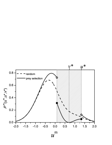
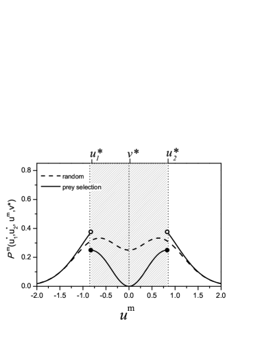
Figure 1: Payoffs for mutant prey under the two predation attack strategies: without prey selection (random; dashed line) and with prey selection (solid line). Left: prey and predator resident populations are monomorphic populations and their phenotypes are set at their stable values, Eq. (5), represented by $u^{*}$and $v^{*}$, respectively. The gray area shows the predator’s preferred phenotype range, where $|u^{\text{m}}-v^{*}|<|u^{*}-v^{*}|$. If we consider a mutant prey whose phenotype is similar to the resident one, the evolutionary outcome will be totally dependent on the predation strategy: The dashed line, obtained from $P_{\text{{random}}}^{\textrm{m}}(u^{*},u^{\text{m}},v^{*})$ in Eq.(6), shows that if predation occurs randomly the mutant phenotype will evolve towards the maximum payoff and then will break the asymmetrical pattern; The solid line, obtained from $P_{\text{{prey\>selection}}}^{\textrm{m}}(u^{*},u^{\text{m}},v^{*})$ in Eq.(7), has two maxima (one when $u^{\text{m}}=u^{*}$and a higher one around $-0.4$), however there is a valley when $u^{m}=v^{*}$ and the higher peak cannot be attained with small mutation steps. Then, only large mutations can break the asymmetrical pattern. Right: prey resident population is dimorphic while predator population is monomorphic and their phenotypes are setting at their stable values, Eq. (10), $u_{1}^{*}$, $u_{2}^{*}$, and $v^{*}$,respectively. The gray area shows the predator’s preferred phenotype range. Both payoff functions, obtained from $P_{\text{{random}}}^{\textrm{m}}(u_{1}^{*},u_{2}^{*},u^{\text{m}},v^{*})$ in Eq (11) and $P_{\text{{prey\>selection}}}^{\textrm{m}}(u_{1}^{*},u_{2}^{*},u^{\text{m}},v^{*})$ in Eq. (12), have two maxima which means that the symmetrical prey branching can be a stable pattern regardless the predator strategy. However, when the predation occurs with preference there is a deeper valley minimizing the flux from one mode to the other. Parameters $\gamma=\alpha=1$.

The consequences of predators preferring certain prey is that in a homogeneous resident prey population, mutant prey that are slightly farther away from the ‘focus’ of the predator are better protected. In the situation depicted in the left graph of Figure (1), the phenotype combination $(v^{*},u^{*})$ is unilaterally optimal (i.e., a Nash equilibrium) and thus an ESS candidate. To the prey, it does not pay to reduce costs by reducing $u^{\text{m}}$, as they would immediately be attacked preferentially, to the predators it does not pay to focus on larger prey because of the balancing selection. There is a higher optimum for the prey, but this cannot be reached by small mutation steps without crossing the adaptive valley. Only when $u^{*}$ and $v^{*}$ are close, mutations may arise that ‘jump’ the valley and thus break the asymmetric pattern. In larger populations or mutation rates, the symmetric pattern is likely to result, but in smaller, stochastic populations, the asymmetric pattern may just switch to the other side.

Dimorphic prey population: Symmetrical branching stability

Assume now a situation where there is a monomorphic predator population, with phenotype $v$, and a dimorphic prey resident population, with phenotypes $u_{1}$ and $u_{2}$. As before, we will look for the stable solution when there is only one prey ( $u_{1}$ or $u_{2}$) in a given predation neighborhood, and then we do not need to impose any selection strategy. The probabilities that prey and predators win the interaction and produce an offspring can be written as

$$P_{v}(u_{1},u_{2},v) = \frac{1}{2}\left\{f_{1}+f_{2}\right\}h_{v}\>,$$ (8)

$$P_{u_{1}}(u_{1},v) = (1-f_{1})h_{u_{1}}\>,$$

$$P_{u_{2}}(u_{2,}v) = (1-f_{2})h_{u2}\>,$$ (9)

where $f_{s}=\exp\left[-\alpha(u_{s}-v^{*})^{2}\right]$ and the term $\nicefrac{{1}}{{2}}$ assume that prey populations occur with equal abundance. Analogous to the previous procedure (however without any approximation), the first and second derivatives allow us to calculate a possible solution

$$u_{1}^{*}=\pm\sqrt{\frac{1}{\alpha}\ln\left(\frac{\alpha+\gamma}{\gamma}\right)};\>u_{2}^{*}=-u_{1}^{*};\>v^{*}=0\>,$$ (10)

that is evolutionarily stable (Fig. S3 in the supplementary material) when $(\alpha+\gamma)>2\alpha\ln\left(\frac{\alpha+\gamma}{\gamma}\right)$ (if we assume $\gamma=1$ , for example, then the condition is $\alpha<1.37$). (For greater values of $\alpha$, $v^{*}=0$ becomes a minimum point and two symmetrical maximum points emerges for $P_{v}(u_{1}^{*},u_{2}^{*},v)$, leading to divergence in the predator population (Vincent and Brown 1989)).

Regarding the stable symmetric pattern, where the phenotypes evolve to $u_{1}^{*}$, $u_{2}^{*}$ and $v^{*}$, we approached the effect of another prey (mutant) in the predation neighborhood, whose phenotype is $u^{\text{m}}$. As before, consider now that a new mutant appears in a given predation neighborhood. Then, there are two prey in this predation neighborhood; a resident ($u_{1}^{*}$ or $u_{2}^{*}$ with equal probability) and a mutant ($u^{\text{m}}$). The probability that the mutant prey is not attacked and produces offspring depends on their phenotypes and on the predator strategy. If predators attack at random,

$$P_{\text{{random}}}^{\textrm{m}} (u_{1}^{*},u_{2}^{*},u^{\text{m}}_{i},v^{*})= \frac{1}{2}\left\{\frac{1}{2}\left[f_{1}+f_{2}+\left(2-f_{1}-f_{2}\right)\left(1-f^{\text{m}}\right)\right]+\left(1-f^{\text{m}}\right)\right\}h^{\text{m}}\>,$$ (11)

otherwise,

$$P_{\text{{prey\>selection}}}^{\textrm{m}}(u_{1}^{*},u_{2}^{*},u^{\text{m}},v^{*})=\begin{cases}\left(1-f_{i}\right)h^{\text{m}}&if\>|u^{\text{m}}-v^{*}|\leq|u^{*}-v^{*}|\\ \frac{1}{2}\left[f_{1}+f_{2}+(2-f_{1}-f_{2})(1-u^{\text{m}})\right]h^{\text{m}}&if\>|u^{\text{m}}-v^{*}|>|u^{*}-v^{*}|\end{cases}\>.$$ (12)

Both payoff functions have two maximum points (see the right graph of Figure 1), which means that the symmetrical prey branching can be a stable pattern regardless of the predator strategy. However, if the predator attacks with prey selection, the two optimum phenotypes for the mutant coincide with the phenotypes of the residents while if the predation occurs randomly they are closer; which means that prey selection can impose a more extreme phenotype when compared to random attack. Moreover, if the predator attacks selectively, the two prey lineages are well separated, $P_{\text{{pref}}}^{\textrm{m}}(u_{1}^{*},u_{2}^{*},u^{\text{m}},v^{*})=0$, and then the flux from one lineage to the other occurs only by large mutations (see Figure 1). If one of the lineages goes extinct, selective predation will probably drive the phenotypic adaptations towards the asymmetrical pattern, while for random predation large mutations are not required for the extinct lineage to reemerge. Payoff functions for the predator and the resident prey are shown at supplementary material (Figure S4).

2.3 Individual Based Model

An Individual Based Model (IBM) was built in order to verify the situations where the asymmetrical pattern is observed. We propose a dynamics where individuals are submitted to both interaction and stabilizing selections and the offspring inherit their parent’s phenotype plus mutation, which allows coevolution of the phenotypes. We model the two predation strategies: with and without prey selection. Some variations of the model assumptions were made to test the robustness of our conclusions and are presented at the "Robustness" subsection below.

We defined a finite population composed by $M_{u}$ prey and $M_{v}$ predators. Space is not modeled explicitly and for simplicity, the model considers synchronized events and a discrete life cycle; in a given generation, the members of both populations first interact and then reproduce to form the next generation. Although space is not explicitly modeled, we assume that each predator $i$ can attack only a subset of $n_{i}$ individuals of the prey population chosen at random, which resembles the limitation of prey in a predator foraging area (predation neighborhood). We assume that the average number of prey in a predation neighborhood is $M_{u}/M_{v}$ with variation among predators. As the number of predators increases, the predation neighborhoods diminish, which models the scenario where predators compete for prey. So, we distribute $M_{u}$ prey (with replacement) over the $M_{v}$ predators (with replacement). As consequence, $n_{i}$ follows a binomial distribution where a prey has a chance of $1/M_{v}$ of being in each predation neighborhood in each one of $M_{u}$ events (see details at supplementary material). We have also explored the situation where $n_{i}$ is a fixed parameter over individuals and over time (see "Robustness" section), and we show that the conclusions highlighted here do not depend on the way this is chosen. In both approaches, one prey can be in more than one predation neighborhood or in no predation neighborhood at all.

After setting the prey for each predator’s neighborhood, all predators that have at least one prey in their predation neighborhood will attack. The sequence of predator attacks is set at random, but once one predator is chosen, it attacks until its first success or until it has tried to attack all prey in its predation neighborhood. The probability of a successful attack is determined by the interaction pressure, Eq. (2). If an attack is successful, the prey dies and the predator will have an opportunity to produce an offspring. A prey can only be successfully attacked once, and if it occurs, the prey is removed from the other predation neighborhoods into which it pertains. This process resembles the interaction between hosts and parasitoids where parasitoids attempt to deposit eggs inside their hosts, but hosts may defend themselves, e.g., by encapsulating the parasitoid egg (Bartlett and Ball 1966), whereas the successful development of the parasitoid results in the death of the prey. We have also considered the situation where the victim does not die, but its fitness is reduced due to the consumer. Again, our highlighted conclusions are robust under this model variation.

Only surviving prey, $M^{\prime}_{u}$, and successful predators, $M^{\prime}_{v}$, will reproduce, and for simplicity we consider asexual reproduction only. The probability of an individual having one offspring depends on how its phenotype is well adapted to the stabilizing selection, Eq. (1). Moreover, in order to have an upper bound in prey population size, it was considered intraspecific competition pressure, resulting in the following probability of a survivor prey having one offspring:

$$g(u_{i}) = \frac{1}{1+\rho(M^{\prime}_{u}-1)}h(u_{i}),$$ (13)

where $\rho$ is a parameter that controls the strength of competition and $h(u_{i})$ is the stabilizing selection, Eq. (1). When there is a unique prey in the whole system there is no competition and $g(u_{1})=h(u_{1})$, while as the population grows $g(u_{i})$ goes to zero. Predator population size is indirectly limited by the size of the prey population, so the probability of each predator $i$, among $M^{\prime}_{v}$ feeding predators, to have one offspring is given by $g(v_{i})=h(v_{i})$, Eq. (1). After all interactions, number of offspring which will recompose the next generation is computed as:

$$M^{\prime\prime}_{s}=F_{s}\sum_{i=1}^{M^{\prime}_{X}}g(s_{i}),$$ (14)

where $F_{s}$ is a parameter that represents the average number of offspring per prey (if $s=u$, or predator if $s=v)$ individual under higher fitness, $h(s_{i}=s_{opt})=1$. The parameter $\rho$, in Eq. (13), can be written in terms of prey carrying capacity ($K$) and $F_{u}$. For that, considering the situation of higher fitness for all $M^{\prime}_{u}$ prey, the number of offspring in the next generation would be:

$$M^{\prime\prime}_{u}=\frac{F_{u}M^{\prime}_{u}}{1+\rho(M^{\prime}_{u}-1)}.$$

When the population achieves the carrying capacity (K), we will have $M^{\prime}_{u}=M^{\prime\prime}_{u}=K$ , which allows us to write:

$$\rho=\frac{F_{u}-1}{K-1}.$$

During the simulation we first calculated the number of offspring, Eq. (14) and then associated each offspring to a parent with probability described in Eq. (13) ( for prey or $g(v_{i})=h(v_{i})$, Eq. (1) for predators). An offspring possesses the same phenotype as its parent plus a normally distributed mutational variation $\delta_{s}$, with

$$P(\delta_{s})=\frac{1}{\sigma_{s}\sqrt{2\pi}}\exp\left[-\frac{\delta_{s}^{2}}{2\sigma_{s}^{2}}\right],$$ (15)

where $\sigma_{s}$ is the standard deviation. The new generation replaces the previous generation ($M_{s}=M"_{s}$), a new set of interactions occurs, the surviving prey and fed predators have offspring, and the cycle restarts. A list of all parameters involved in the model is shown in Table (1).

Table 1: List of all parameters involved in the model, their values utilized in the simulations and a short description of their meaning

parameter	value	short meaning
$\alpha$	{1, 2, 4, 6, 8, 10, 20, 40, 100, 1000}	Intensity of selection imposed by the interaction
$\gamma_{u};\gamma_{v}$	1	Intensity of stabilizing selection pressure
$u_{opt};\>v_{opt}$	0	Optimum phenotype imposed by the stabilizing selection
$F_{u};\>F_{v}$	{2, 4, 6, 8, 10, 12}	Fecundity
$K$	{500, 2000, 5000, 10000, 50000}	Prey carrying capacity
$\sigma_{u};\>\sigma_{v}$	{0.01, 0.02}	Standard deviation that defines the mutation amplitude

2.3.1 Scenarios

We investigated the coevolutionary patterns (phenotype distributions over the generations) and population sizes for both models (with prey selection and without prey selection) considering different parameter combinations (see Table1) but we fixed the strength of stabilizing selection and the optimum phenotype favored in absence of the interaction ($\gamma_{u}=\gamma_{v}=1;\;u_{opt}=v_{opt}=0$). For all simulations the initial condition corresponded to one thousand individuals of each trophic level and phenotype values were equal to the optimum phenotype imposed by the stabilizing selection, plus a normally distributed variation (as in Eq.15). Each simulation was iterated over ten thousand generations.

2.3.2 Robustness

To assess the robustness of our results we analyzed some modifications to the model assumptions. The modifications and results are outlined below (and detailed in the supplementary material).

We modeled the antagonistic interaction by promoting a fitness benefit for the exploiter and a fitness prejudice for the victim instead of death due to interaction. The benefit and prejudice are controlled by two independent parameters, which allows to analyze the effect of different impacts on each trophic level. For simplicity, the population size of each trophic level remained constant, then the contribution of each individual to the next generation population was proportional to its individual fitness. The number of victim in an exploiter’s attack neighborhood was a fixed parameter and the interaction occurs only with one individual. As in the original model, we investigate two scenarios: (i) attack occurs at random; (ii) exploiters can select a victim according to phenotype matching. We ran simulations for 400 combinations of parameters for each scenario (with and without prey selection): we qualitatively predict the same coevolutionary patterns observed originally, including the exclusivity of the asymmetrical pattern for the second scenario (See Figures S7 and S8, in the supplementary material).

3 Simulation results

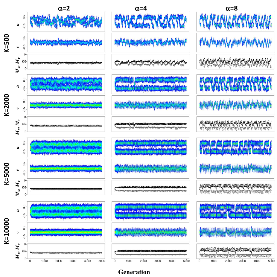
Figure 2: Coevolutionary temporal patterns for the model without prey selection and with different intensities of interaction strength ($\alpha$, in columns) and carrying capacity ($K$, in rows). The first two graphs of each set of three sequential graphs show prey ($u$) and predator ($v$) phenotype temporal evolution, respectively. The color scale is proportional to the number of individuals with a given phenotype (from blue to red meaning low to high frequencies). The bottom graph shows the prey (black) and predator (gray) population size over time. Only the last three values of $K$ correspond to the same parameter values present in Figure 3. Parameters: $\gamma=1,$ $u_{opt}=v_{opt}=0$, $F_{u}=8$, $F_{v}=2$, $\sigma_{u}=\sigma_{v}=0.02$.

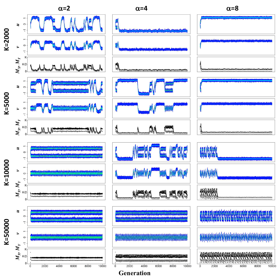
Figure 3: Coevolutionary temporal patterns for the model with prey selection and considering different intensities of interaction ($\alpha$, in columns) and carrying capacity ($K$, in rows). The first two graphs of each set of three sequential graphs show prey ($u$) and predator ($v$) phenotype temporal evolution, respectively. The color scale is proportional to the number of individuals with a given phenotype (from blue to red meaning low to high frequencies). The bottom graph shows the prey (black) and predator (gray) population size over time. Only the first three values of $K$ correspond to the same parameter values present in Figure 2. Parameters: $\gamma=1,$ $u_{opt}=v_{opt}=0$, $F_{u}=8$, $F_{v}=2$, $\sigma_{u}=\sigma_{v}=0.02$.

Both models were sensitive to the interaction strength ($\alpha$) and the carrying capacity ($K$) (Figures 2 and 3). Higher values of $\alpha$ lead to a more intense selection in the predator population whose phenotypes better matches their prey phenotypes. From the prey point of view, the pressure results in the differentiation of their phenotypes from the predator population. The condition of attacks with prey selection, Figure 3, has similar effects to increasing interaction selection, but the evolutionary pattern observed under this strategy cannot always be recovered by increasing the interaction strength ($\alpha$) in the model without prey selection, Figure 2 (detailed below). The carrying capacity is also an important parameter for the evolutionary outcomes since smaller populations are more vulnerable to demographic stochasticity and extinction (Figures 2 and 3). Once prey selection increases the pressure on prey, the minimum value of $K$ to observe predator and prey coexistence is higher when compared to the attacks without prey selection (Observe that the minimum value of $K$ differs between Figures 2 and 3).

We qualitatively classify three different patterns for the population phenotype distribution across the generations: symmetrical coevolutionary oscillations, symmetrical coevolutionary branching and asymmetrical pattern. In symmetrical coevolutionary oscillations, prey and predator phenotypes oscillate around the respective optimum values in absence of the interaction (as an example see Figure 2 when $K=500$ and $\alpha=8$ and Figure 3 when $K=2000$ and $\alpha=2$). In this scenario, neither population reaches an equilibrium phenotype distribution. Occasionally a bifurcation in the distribution of the prey phenotype appears that last for a few generations but that will eventually disappear again when one of the branches goes extinct. In the symmetrical coevolutionary branching pattern, prey phenotypes bifurcate between two lineages with phenotype values symmetric in relation to the optimum phenotype imposed by the stabilizing selection, while the predator phenotypes assume values between both lineages and around $v_{opt}=0$ (as an example see Figures.2 when $K=10000$ and $\alpha=\{2,4\}$ and 3 when $K=50000$ and $\alpha=\{2,4\}$). Finally, the asymmetrical pattern was observed exclusively in the model with prey selection. Both prey and predator phenotypes evolve to values above or below (some simulations can result above while another simulation with same parameters can result below) the static optimum phenotype imposed by stabilizing selection but without tallying up; predator phenotypes stay between the prey phenotype and the optimum phenotype imposed by the stabilizing selection (see Figure 3 when $(K;\alpha)=\{(2000;4),$$(2000;8),$ $(5000;8),$ $(10000;8)\}$). In agreement with our analytical approach, predators that can selectively attack a preferred prey can lock the prey phenotype in one of the two stable phenotypes. Any prey mutant that tries to cross towards the other stable phenotype becomes the preferred prey, which minimizes its reproductive success. When the attack is random (without prey selection) that mutant prey will never be preferentially attacked. We have also tested if the asymmetry would emerge by increasing the interaction strength when the attack is random ($\alpha$={10, 20, 40, 100, 1000}, Figure S5), but it resulted in prey extinction or high frequency phenotype oscillations. We have also confirmed this result under variation of model assumptions, see the Robustness section above.

We also calculated the maximum time that the prey phenotypes stay in asymmetry. For that, from generation 3,000 to 10,000 we calculated the maximum time that the average prey phenotype did not cross zero. We then calculated the average time over 10 replicates (Figure 4 and Figure S6). Only in the dynamics with preference some parameters combinations resulted in 7,000 generations (100% of analyzed time) in asymmetry for all repetitions. The maximum time that we could observe asymmetry when prey selection is not considered was about 125 generations (for other parameter combinations we could observe almost 300 generations, see Figure S6), which is actually the period of cycling phenotypes, not stable asymmetry. If we fix a $K$ value and increase $\alpha$, we have an increase of the time in asymmetrical pattern up to a certain $\alpha$ value; from that value on, populations are extinct or the phenotypes oscillate in high frequency (it occurs for both models, see Figure 4 for $\alpha=\{100,1000\}$). The high frequency oscillations probably occur because the standard deviation of the interaction selection ($\sim\nicefrac{{1}}{{\sqrt{\alpha}}}$, see Eq.2) approaches the mutation standard deviation $\sigma$ (Eq.15). It means a higher probability of a survivor prey having a descendant out of the predator phenotype requirements.

If we consider a given interaction strength $\alpha>0$ and observe the patterns as a function of $K$, we first have extinction of predators or of both populations (not shown in Figures 2 and 3, but in Figure S5 and Figure 4, where higher values of $\alpha$ are considered). As population densities increase, predator and prey populations coexist going through the following patterns: asymmetrical pattern (only in the model with prey selection), coevolutionary oscillation and finally symmetrical branching (as an example see Figure 3 when $\alpha=4$). In the transitions between these patterns we may have combinations of them, for instance with populations that oscillate, bifurcate and have lineages that go extinct and emerge again (see Figure 2 when $K=500$ and $\alpha=4$ and Figure 3 when $K=10000$ and $\alpha=4$, for example). A similar sequence of coevolutionary patterns occurs if we consider a given value $K$ and decrease $\alpha$.

In addition to the asymmetrical pattern, prey selection produces more extreme evolutionary dynamics compared to the random predation model: the phenotypes evolve to values further from the optimum set by stabilizing selection (even if we compare high $\alpha$ in the model without prey selection with low $\alpha$ in the model with prey selection), decreasing the fitness of both populations. As a consequence, extinction is more likely to happen when predators attack with prey selection under low prey carrying capacity. For example, when $K=500$ either predators or both predator and prey populations become extinct for any value of $\alpha$, while in the model without prey selection we observe coevolutionary oscillation (see Figure 2 when $K=500$). Coevolutionary oscillation also appears in the model with prey selection for higher values of $K,$ resulting in oscillations with higher amplitude and periods (compare Figure 2 when $K=500$ and $\alpha=2$ to Figure 3 when $K=2000$ and $\alpha=2$).

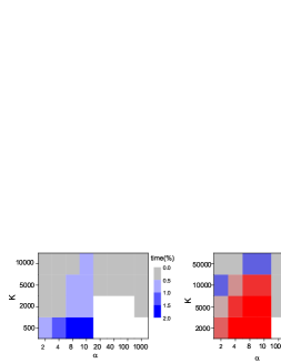
Figure 4: Average of the longest time in asymmetrical pattern as function of the interaction strength $(\alpha)$ and carrying capacity ($K$) for the model without prey selection(left) and with prey selection (right). For each parameter combination was analyzed the longest time in asymmetry for 7000 generations (from generation 3,000 to 10,000). The average was calculated over 10 replicates. The graphs show the percentage (from 0 to 100% of analyzed time in asymmetry). White area means extinction of at least one of the populations for all replicates. Observe that the graphs have different color scales; the model without prey selection does not maintain the asymmetry for more than 2% of analyzed time, which corresponds to about 125 generations, while the model with prey selection the asymmetry can be maintained for all analyzed time.

Population size fluctuations arise in particular under non-equilibrium dynamics of phenotype evolution (coevolutionary oscillation and in the transition between patterns) while a more constant population size was associated with stable phenotype evolutionary patterns (asymmetrical pattern and symmetrical branching) (Figure 2 and 3). Although asymmetrical pattern leads to a constant population size, predator population size was lowest in these cases, making it more vulnerable to extinction (by increasing the interaction strength or imposing a perturbation). We also computed the mean size of the predation neighborhood, $\left\langle n\right\rangle=\left\langle M_{u}/M_{v}\right\rangle$ and mean relative population densities, $\left\langle M_{u}\right\rangle/K$ and $\left\langle M_{v}\right\rangle/K$, calculated from the last 7000 generations of each simulation (Figure 5). Both population densities tend to converge for a given interaction strength ($\alpha$), as the carrying capacity increases. Prey populations remain sensitive to the intensity of interaction regardless of the predators’ strategy, whereas predator populations are sensitive only if they attack at random; if predators attack preferentially certain prey, their density seems to converge to the same point independently of $\alpha$. Consequently, the predation neighborhood increases with the intensity of the interaction. For high values of $K$, prey selection leads to a slightly larger mean predation neighborhood. For low values of $K$, where the asymmetrical pattern occurs, both population densities are reduced, but the predator population diminishes more drastically. In compensation, the predation neighborhood increases so that the few predators have more prey to choose from (see the highlighted dots in Figure 5).

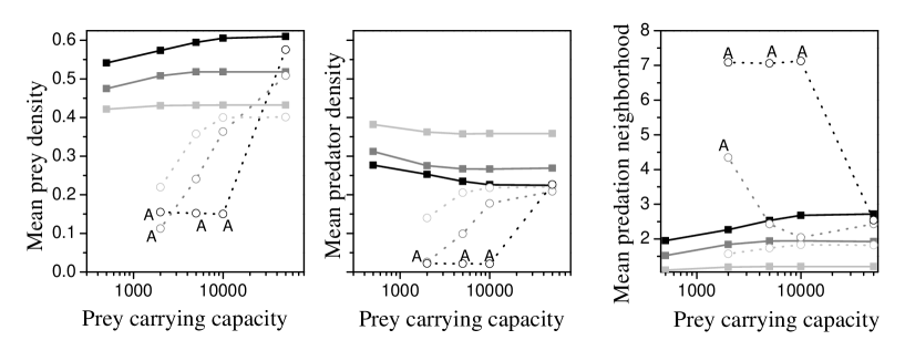
Figure 5: From left to right: Prey and predator population densities, $\left\langle M_{u}\right\rangle/K$ and $\left\langle M_{v}\right\rangle/K$, and mean size of the predation neighborhood, $\left\langle n\right\rangle=\left\langle M_{u}/M_{v}\right\rangle$, as function of prey carrying capacity, $K$. The filled squares refer to the scenario where predators attack at random (without prey selection) while the open circles to the scenario with prey selection (the first point, $K=500$, is not plotted for the case with prey selection because predator and prey do not coexist). These averages were computed considering the last $7000$ of $10000$ generations. The colors, light gray, gray and black correspond to $\alpha$ equal to $2$, $4$ and $8,$ respectively. The letter "A" highlight the parameter combinations where the asymmetrical pattern occurs.

4 Discussion

We investigated the coevolutionary dynamics of predator-prey systems in which predators can choose which prey to attack in their immediate neighborhood. The interaction selection was considered non-directional; only the difference between prey and predator phenotype determines predation success. However, in addition to a situation in which predators encounter prey only randomly, we also allow them to select prey to attack from prey present in their predation neighborhood, where they will preferentially attack prey with the closest match. We compare the individuals’ payoffs and the temporal population phenotype distributions – coevolutionary patterns – for a number of different parameter combinations and also under different model assumptions (Robustness section), that represent different ecological settings. Our results support four main conclusions described below.

First, trait evolution is sensitive to the intensity of interaction selection and the populations’ carrying capacity. For a given value of interaction strength, increasing the carrying capacity has the following effects: at small abundances, we have extinction of predators or both populations; as population densities increase, they tend to coexist indefinitely, shifting through the following patterns: asymmetrical pattern (which occurs only in the model with prey selection), symmetrical coevolutionary oscillation and finally symmetrical branching. The term "symmetry" means that, along time, phenotypes occupied both regions delimited by the optimum phenotype with equal amplitude. In the transition between patterns, these are combined with populations oscillating, bifurcating and forming lineages that go extinct and then evolve again. A similar sequence of coevolutionary patterns occurs with a fixed carrying capacity and decreasing interaction strength. With symmetrical branching, the prey evolves to a bimodal phenotype distribution, while the predator evolves to an intermediate phenotype which is equally effective against both prey lineages. The coevolutionary oscillatory pattern is related to Red Queen evolution (van Valen, 1973), where rare prey phenotypes are more likely to evade predation and thus phenotype frequencies in prey populations change continuously, while the predators keep evolving to specialize on the most common prey types (Dieckmann et al. 1995). It should be noted however, that the oscillatory pattern observed under prey selection is somewhat different, and results from the episodic reversal between two stable patterns. In contrast to van Valen’s Red Queen dynamics, this oscillatory pattern strongly depends on population sizes, as it depends on the frequency of those rare mutations that manage to cross the adaptive valley driven by predators selectively attacking preferred prey. It is interesting to note that the simulation has not shown predator phenotype branching (following the prey branching) that would emerge, according to Brown and Vincent’s study (1992) and also by our analytical approach, when the interaction strength increases. Instead, as the interaction strength increases, we observed symmetrical coevolutionary oscillation. We did not explore the reason of it, but we propose that this pattern still may emerge outside the parameter space we explored, probably by decreasing the intensity of stabilizing selection and then allowing for a wider range of phenotypes. Future studies should be done in order to clarify it.

Both stable and unstable patterns have been predicted by many theoretical models (Gomulkiewicz et al. 2000; Abrams 2000; Dieckmann et al. 1995; Levin and Udovic 1977; Thompson 2005; Brown and Vincent 1992; Calcagno et al. 2010), although empirical examples remain sparse. The presence of bimodal host phenotype distributions have been empirically observed in a natural Daphnia population during a parasite epidemic (Duffy et al. 2008) and also in host egg coloration subject to avian brood parasitism (Yang et al. 2010). Empirical evidence of an oscillating pattern was again found in host egg colorations and their avian brood parasite by Spottiswoode and Stevens (2013) and in a herbivorous moth and its host plant (Berenbaum and Zangerl 1998). Frequency-dependent selection between populations has already been pointed by Levin and Udovic (1977) as an important driver in evolutionary history. In agreement with these authors, we verified that selective pressure in smaller populations can lead to different evolutionary effects from those expected in larger populations.

Second, both the analytical approach and IBM simulations agree that prey selection causes prey phenotypes to evolve towards more extreme values than randomly attacking predators. When the resulting evolutionary pattern is oscillatory, its amplitude is higher and when prey phenotypes bifurcate, the stable phenotypes are more extreme. This higher differentiation between phenotypes in the branching pattern suggests that selective predation can facilitate speciation. This would be caused if phenotypic differentiation was followed by reproductive isolation (Dieckmann and Doebeli, 1999). The current model does not allow for this additional evolutionary step, as reproductive isolation makes no sense under the assumption of asexual reproduction. Future studies, expanding this model to include sexual reproduction and reproductive isolation could test the effect of the resource selection strategy on diversification rates in order to validate this prediction.

Third, prey selection makes predators more efficient which paradoxically, reduces at least the predator population size. Other models of exploitative interactions have found that enhancing a consumer’s efficiency reduces its population density (Peterson 1984). In our model, for a sufficiently high carrying capacity, the predator strategy has no effect on prey density, or on the ensuing evolutionary pattern: in both strategies the system converges to symmetrical branching at high carrying capacity (although the stable prey phenotypes are more divergent under selective predation). However, under low carrying capacity, the predator density decreases when there is prey selection (see Figure 5), and as a consequence, the predation neighborhood increases (since it is proportional to the ratio of prey and predator population sizes). Predator population size is reduced under selective versus random predation, probably because selective predation imposes a higher pressure on prey phenotype, which in turn exerts a higher pressure on predators. In a first instance, for a given prey phenotype distribution, prey selection increases predator success, but over evolutionary time it reduces the predator population benefit compared to random predation. At low values of carrying capacity, both populations are more vulnerable to extinction when predation is selective. This issue is particularly important regarding species that evolve in islands, in fragmented patches or that naturally occur in low abundance.

Fourth, an asymmetrical pattern can emerge unexpectedly. Usually, when there is a stabilizing selection that bounds the prey and predator phenotype distributions around the same optimum value and the interaction pressure is non-directional (phenotype matching, which promotes bidirectional axis of vulnerability, as approached by Abrams (2000)), the expected emerged patterns for the coevolving species are symmetric; oscillating or bifurcating in two or more lineages (around an optimal value imposed by the stabilizing selection). For species phenotypes to coevolve in asymmetry, the expected mechanism would be directional pressure, phenotype difference, which promotes an unidirectional axis of vulnerability (Abrams 2000). Here we showed that non-directional pressure (phenotype matching) associated to prey selection can limit prey phenotypes to an asymmetrical pattern, which can only be broken if population densities increase. In accordance with the analytical results, the model variation presented in the supplementary material showed that the asymmetrical pattern is not unique to the set of assumptions made in the model presented here at the main text. There, population density does not vary trough time (extinction is not allowed) but impacts the fitness of populations. The main common assumptions made in both model variations were the presence of a predation neighborhood and the predator satiation (once it successfully attacks a prey, it stops attacking). These assumptions are the key for what makes the predator strategy relevant: if an optimum prey is in a predation neighborhood, its fate is to be attacked if the predator strategy considers prey preference. However, if the predator attacks randomly, that prey can go unnoticed. It means that predators that can selectively attack a preferred prey can lock the prey phenotype in one of the two stable phenotypes. Any prey mutant that tries to cross towards the other stable phenotype becomes the preferred prey, which minimizes its reproductive success. Although, to our knowledge, asymmetrical patterns have not been documented before in the conditions mentioned above, such patterns can be observed in absence of stabilizing selection (Calcagno et al. 2010) and also in models of specialization on two habitats, where strong fitness trade-offs can produce specialists in only one habitat (then asymmetrical) (Levins 1962; Rueffler et al. 2004; Ravigne et al. 2009). Our analytical model shows the importance of sharp decrease in the probability of survival of the prey under prey preference, when the phenotype of the mutant is closer to the predator phenotype than the resident phenotype. This situation can occur when there is a slight difference between the prey phenotypes, and the predator prefers the phenotype that gives it the greatest fitness contribution, even if the difference is very small. This discontinuity may be not realistic, since in a predation neighborhood a small phenotypic variation may not be noticed by the predator. As a consequence, a mutant can no longer ‘hide’ behind more preferred prey, and the asymmetrical pattern would be broken more easily. However, we expect that the asymmetrical pattern persists, but less pronounced. Moreover, we have not explored other interaction and stabilizing functions that were not Gaussian, (Eqs. (1) and (2)). Then, the generalization of our results for other symmetrical functions remains open. Further study should assess the generalization of it as well as which level of differentiation by the predator is necessary to produce asymmetrical patterns.

Our study can shed light on currently observed evolutionary patterns, and a prime example is the evolution of egg morphology of cuckoo brood parasites and their hosts. This system presents the two elements we are highlighting: non-random host selection (parasite individuals choose the nest where they will lay eggs) and non-directional pressure (parasite success increases with phenotype matching) (Avilés et al. 2006; Soler et al. 2014). The study by Spottiswoode and Stevens (2013) compared the appearance (color and patterns) of cuckoo finch eggs with their hosts, the tawny-flanked prinia (Prinia subflava) from the same location in Zambia over 40 years. As mentioned before, they found that egg colors seem to be locked in an ongoing arms race (symmetrical coevolutionary cycling). However, part of the egg color pattern traits measured have been changing their mean values, accompanied by decreases in phenotypic variation, suggesting directional selection (evolving to an asymmetrical pattern which the authors interpreted as resulting from some undetected directional pressure which would drive this asymmetrical evolution). Our model provides an alternative explanation for this result, which requires no other pressure besides the host selection by brood parasites according to phenotypic-matching; the observed pattern emerges directly from this non-random interaction.

In conclusion, our results bolster the conclusion that non-random interactions can have important ecological and evolutionary consequences. This ubiquitous behavioral aspect of antagonistic interactions had so far been ignored in co-evolutionary models, and this study shows that in addition to the long known ecological consequences prey selection also has unexpected evolutionary consequences, such as generating striking asymmetrical (or cyclic) evolutionary outcomes. Our results are also a reminder to keep considering the ecological context in evolutionary dynamics, as our results are most pronounced under those ecological conditions where population sizes are relatively low.

References

- Abrams (2000) Abrams, P. A. 2000. The Evolution of Predator-Prey Interactions: Theory and Evidence. Annual Review of Ecology and Systematics 31:79–105.
- Abrams and Kawecki (1999) Abrams, P. A., and T. J. Kawecki. 1999. Adaptive host preference and the dynamics of host-parasitoid interactions. Theor. Pop. Biol. 56:submitted.
- Andreazzi et al. (2017) Andreazzi, C. S., J. N. Thompson, and P. R. Guimarães. 2017. Network Structure and Selection Asymmetry Drive Coevolution in Species-Rich Antagonistic Interactions. The American Naturalist 190:99–115.
- Avilés et al. (2006) Avilés, J. M., B. G. Stokke, A. Moksnes, E. Røskaft, M. Asmul, and A. P. Møller. 2006. Rapid increase in cuckoo egg matching in a recently parasitized reed warbler population. Journal of evolutionary biology 19:1901–10.
- Bartlett and Ball (1966) Bartlett, B. R., and J. C. Ball. 1966. The Evolution of Host Suitability in a Polyphagous Parasite with Special Reference to the Role of Parasite Egg Encapsulation 1. Annals of the Entomological Society of America 59:42–45.
- Berec (2000) Berec, L. 2000. Mixed encounters, limited perception and optimal foraging. Bull. Math. Biol. 62:849—868.
- Berenbaum and Zangerl (1998) Berenbaum, M. R., and A. R. Zangerl. 1998. Chemical phenotype matching between a plant and its insect herbivore. Proceedings of the National Academy of Sciences 95:13743–13748.
- Brown and Vincent (1992) Brown, J. S., and T. L. Vincent. 1992. Organization of Predator-Prey Communities as an Evolutionary Game. Evolution 46:1269–1283.
- Calcagno et al. (2010) Calcagno, V., M. Dubosclard, and C. de Mazancourt. 2010. Rapid exploiter-victim coevolution: the race is not always to the swift. The American Naturalist 176:198–211.
- Chew (1977) Chew, F. S. 1977. Coevolution of Pierid Butterflies and Their Cruciferous Foodplants . II . The Distribution of Eggs on Potential Foodplants. Evolution 31:568–579.
- Dieckmann and Doebeli (1999) Dieckmann, U., and M. Doebeli. 1999. On the origin of species by sympatric speciation. Nature 400:354–357.
- Dieckmann et al. (1995) Dieckmann, U., P. Marrow, and R. Law. 1995. Evolutionary cycling in predator-prey interactions: population dynamics and the red queen. Journal of theoretical biology 176:91–102.
- Duffy et al. (2008) Duffy, M. A., C. E. Brassil, S. R. Hall, A. J. Tessier, C. E. Caceres, and J. K. Conner. 2008. Parasite-mediated disruptive selection in a natural Daphnia population. BMC Evol Biol 8:80.
- Ehrlich and Raven (1964) Ehrlich, P. R., and P. H. Raven. 1964. Butterflies and plants: a study in coevolution. Evolution pages 586–608.
- Fryxell and Lundberg (1994) Fryxell, J. M., and P. Lundberg. 1994. Diet choice and predator-prey dynamics. Evol. Ecol. 8:407–421.
- Gandon and Michalakis (2002) Gandon, S., and Y. Michalakis. 2002. Local adaptation, evolutionary potential and host-parasite coevolution: interactions between migration, mutation, population size and generation time. Journal of Evolutionary Biology 15:451–462.
- Gendron (1987) Gendron, R. P. 1987. Models and mechanisms for frequency-dependent predation. Am. Nat. 130:603–623.
- Gleeson and Wilson (1986) Gleeson, S. K., and D. S. Wilson. 1986. Equilibrium diet: optimal foraging and prey coexistence. Oikos 46:139–144.
- Gokhale et al. (2013) Gokhale, C. S., A. Papkou, A. Traulsen, and H. Schulenburg. 2013. Lotka-Volterra dynamics kills the Red Queen: population size fluctuations and associated stochasticity dramatically change host-parasite coevolution. BMC evolutionary biology 13:254.
- Gomulkiewicz et al. (2000) Gomulkiewicz, R., J. N. Thompson, R. D. Holt, S. L. Nuismer, and M. E. Hochberg. 2000. Hot Spots, Cold Spots, and the Geographic Mosaic Theory of Coevolution. The American Naturalist 156:156–174.
- Hochberg and van Baalen (1998) Hochberg, M. E., and M. van Baalen. 1998. Antagonistic coevolution over productivity gradients. The American naturalist 152:620–34.
- Hutson (1984) Hutson, V. 1984. Predator mediated coexistence with a switching predator. Math. Biosci. 68:233–246.
- Janzen (1980) Janzen, D. H. 1980. When is it Coevolution? Evolution 34:611–612.
- Jorge et al. (2014) Jorge, L. R., P. I. Prado, M. Almeida-Neto, and T. M. Lewinsohn. 2014. An integrated framework to improve the concept of resource specialisation. Ecology Letters 17:1341–1350.
- Levin and Udovic (1977) Levin, S. A., and J. D. Udovic. 1977. A Mathematical Model of Coevolving Populations. The American Naturalist 111:657–675.
- Levins (1962) Levins, R. 1962. Theory of Fitness in a Heterogeneous Environment. I. The Fitness Set and Adaptive Function. The American Naturalist 96:361–373.
- Martín-Gálvez et al. (2006) Martín-Gálvez, D., J. J. Soler, J. G. Martínez, A. P. Krupa, M. Richard, M. Soler, A. P. Møller, and T. Burke. 2006. A quantitative trait locus for recognition of foreign eggs in the host of a brood parasite. Journal of evolutionary biology 19:543–50.
- Matsuda (1985) Matsuda, H. 1985. Evolutionarily stable strategies for predator switching. J. Theor. Biol. 115:351–366.
- May (1974) May, R. M. 1974. Stability and Complexity in Model Ecosystems. Monographs in Population Biology, 2nd ed. Princeton University Press, Princeton NJ.
- Merrill et al. (2013) Merrill, R. M., R. E. Naisbit, J. Mallet, and C. D. Jiggins. 2013. Ecological and genetic factors influencing the transition between host-use strategies in sympatric Heliconius butterflies. Journal of evolutionary biology 26:1959–67.
- Metz et al. (1992) Metz, J. a., R. M. Nisbet, and S. a. Geritz. 1992. How should we define ’fitness’ for general ecological scenarios? Trends in ecology & evolution (Personal edition) 7:198–202.
- Murdoch (1969) Murdoch, W. W. 1969. Switching in general predators: experiments on predator specificity and stability of prey populations. Ecol. Monogr. 39:335–354.
- Noh et al. (2018) Noh, H. J., R. Gloag, and N. E. Langmore. 2018. True recognition of nestlings by hosts selects for mimetic cuckoo chicks. Proceedings of the Royal Society B: Biological Sciences 285.
- Nuismer and Thompson (2006) Nuismer, S. L., and J. N. Thompson. 2006. Coevolutionary alternation in antagonistic interactions. Evolution 60:2207–17.
- Nylin et al. (2005) Nylin, S., G. H. Nygren, J. J. Windig, N. Janz, and A. Bergström. 2005. Genetics of host-plant preference in the comma butterfly Polygonia c-album ( Nymphalidae), and evolutionary implications. Biological Journal of the Linnean Society 84:755–765.
- Peterson (1984) Peterson, S. C. 1984. Herbivory. the dynamics of animal-plant interactions. michael j. crawley. The Quarterly Review of Biology 59:496–496.
- Ravigne et al. (2009) Ravigne, V., U. Dieckmann, and I. Olivieri. 2009. Live Where You Thrive : Joint Evolution of Habitat Choice and Local Adaptation Facilitates Specialization and Promotes Diversity. The American Naturalist 174:141–169.
- Refsnider and Janzen (2010) Refsnider, J. M., and F. J. Janzen. 2010. Putting Eggs in One Basket: Ecological and Evolutionary Hypotheses for Variation in Oviposition-Site Choice. Annual Review of Ecology, Evolution, and Systematics 41:39–57.
- Resetarits (1996) Resetarits, W. J. 1996. Oviposition Site Choice and Life History Evolution. American Zoologist 36:205–215.
- Rothstein (1990) Rothstein, S. I. 1990. A model system for coevolution: avian brood parasitism. Annual Review of Ecology and Systematics 21:481–508.
- Rueffler et al. (2004) Rueffler, C., T. J. Van Dooren, and J. A. Metz. 2004. Adaptive walks on changing landscapes: Levins’ approach extended. Theoretical Population Biology 65:165–178.
- Soler et al. (2014) Soler, J. J., J. M. Avilés, D. Martín-Gálvez, L. de Neve, and M. Soler. 2014. Eavesdropping cuckoos: further insights on great spotted cuckoo preference by magpie nests and egg colour. Oecologia 175:105–15.
- Spottiswoode and Stevens (2013) Spottiswoode, C. N., and M. Stevens. 2013. Host-Parasite Arms Races and Rapid Changes in Bird Egg Appearance. The American Naturalist 179:633–648.
- Stephens and Krebs (1986) Stephens, D. W., and J. R. Krebs. 1986. Foraging Theory. Monographs in Behavior and Ecology. Princeton University Press, Princeton, NJ.
- Taylon and Jonker (1978) Taylon, P. D., and L. B. Jonker. 1978. Evolutionarily Stable Strategies and Game Dynamics. Mathematical Biosciences 40:145–156.
- Thompson (2005) Thompson, J. N. 2005. The geographic mosaic of coevolution. University of Chicago Press, Chicago.
- van Baalen et al. (2001) van Baalen, M., V. Krivan, P. C. J. van Rijn, and M. W. Sabelis. 2001. Alternative food, switching predators, and the persistence of predator-prey systems. Am. Nat. 157:512–524.
- van Valen (1973) van Valen, L. 1973. A new evolutionary law. Evolutionary theory 1:1–10.
- Vincent and Brown (1989) Vincent, T. L., and J. S. Brown. 1989. The Evolution Reponse of Systems to a Changing Environment. Applied Mathematics and Computation 32:185–206.
- Yang et al. (2010) Yang, C., W. Liang, Y. Cai, S. Shi, F. Takasu, A. P. Møller, A. Antonov, F. Fossøy, A. Moksnes, E. Røskaft, and B. G. Stokke. 2010. Coevolution in action: Disruptive selection on egg colour in an avian brood parasite and its host. PLoS ONE 5:1–8.
- Yoder and Nuismer (2010) Yoder, J. B., and S. L. Nuismer. 2010. When Does Coevolution Promote Diversification? The American Naturalist 176:000–000.