Abstract

We discuss the local (gauged) Weyl symmetry and its spontaneous breaking and apply it to model building beyond the Standard Model (SM) and inflation. In models with non-minimal couplings of the scalar fields to the Ricci scalar, that are conformal invariant, the spontaneous generation by a scalar field(s) vev of a positive Newton constant demands a negative kinetic term for the scalar field, or vice-versa. This is naturally avoided in models with additional Weyl gauge symmetry. The Weyl gauge field $\omega_{\mu}$ couples to the scalar sector but not to the fermionic sector of a SM-like Lagrangian. The field $\omega_{\mu}$ undergoes a Stueckelberg mechanism and becomes massive after “eating” the (radial mode) would-be-Goldstone field (dilaton $\rho$) in the scalar sector. Before the decoupling of $\omega_{\mu}$, the dilaton can act as UV regulator and maintain the Weyl symmetry at the quantum level, with relevance for solving the hierarchy problem. After the decoupling of $\omega_{\mu}$, the scalar potential depends only on the remaining (angular variables) scalar fields, that can be the Higgs field, inflaton, etc. We show that a successful inflation is then possible with one of these scalar fields identified as the inflaton. While our approach is derived in the Riemannian geometry with $\omega_{\mu}$ introduced to avoid ghosts, the natural framework is that of Weyl geometry which for the same matter spectrum is shown to generate the same Lagrangian, up to a total derivative.

1 Introduction

In this letter we discuss the Weyl gauge symmetry and its spontaneous breaking together with its implications for model building beyond the Standard Model (SM) and for inflation.

One phenomenological motivation relates to the observation that the SM with a Higgs mass parameter set to zero has a classical scale symmetry [1]. If this symmetry is preserved at the quantum level by (a scale-invariant) UV regularisation as in [2, 3, 4, 5, 6, 7], and is broken spontaneously only, it can naturally protect at the quantum level a hierarchy of fields vev’s of the theory [3, 8, 6, 9, 10]. The hierarchy we refer to is that between the Higgs field vev (electroweak scale) and that of “new physics” represented by the vev of the flat direction (dilaton) associated with global scale symmetry breaking. Such hierarchy of vev’s can be generated by a classical hierarchy of the dimensionless couplings of the theory [11, 12].

A proper study of the hierarchy problem, based on the above idea, demands including gravity and generating spontaneously the Planck scale ($M_{p}$). This can be done in Brans-Dicke-Jordan theories of gravity [13] via a non-minimal coupling between a scalar field(s) and the scalar curvature ($R$), when this field(s) develops a non-zero vev. However, demanding the theory be conformal invariant and spontaneous-only breaking of the conformal symmetry, leads to a negative kinetic term for the corresponding scalar field, a “nuisance” that is often quietly glided over. This problem is automatically avoided in models with Weyl gauge symmetry [14, 15] and motivated our study of this symmetry in Sections 2 and 3.

The Weyl gauge symmetry is the natural extension for conformal invariant models e.g. [14, 15, 16, 17, 13, 18, 19, 20, 21, 22, 24, 25, 26, 27, 23, 28, 29, 30, 31, 32]; the conformal transformation of the metric is extended by the associated gauge transformation of a Weyl gauge field ($\omega_{\mu}$) which is of geometric origin. Section 3 discusses how $\omega_{\mu}$ undergoes a Stueckelberg mechanism and becomes massive by “eating” the would-be-Goldstone field (dilaton $\rho$); here, the dilaton is the radial direction in the field space of scalar fields ($\phi_{j}$) of different non-minimal couplings $\xi_{j}$ to $R$. The Weyl gauge symmetry is then spontaneously broken and there are no negative kinetic terms in the theory. The vacuum expectation value $\langle\rho\rangle$ of the flat direction (dilaton) controls the mass of $\omega_{\mu}$ and $M_{p}$. After $\omega_{\mu}$ decouples, the potential depends only on the remaining angular variables scalar fields which can account for the Higgs field, inflaton, etc. Our analysis extends previous studies [19, 20, 21, 22, 23] to multiple scalar fields ($\phi_{j}$) and different non-minimal couplings ($\xi_{j}$).

We also show (Section 3.4) how prior to this symmetry breaking the dilaton can enforce a UV regularization of the quantum corrections that keeps manifest the Weyl symmetry. In Weyl-invariant models the dilaton replaces the subtraction scale, thus maintaining this symmetry at the quantum level [2, 3, 4, 5, 6, 7], after which is “eaten” by $\omega_{\mu}$ and disappears from the spectrum. One is left with the potential for angular variables fields (e.g. Higgs field, etc). This is relevant for the hierarchy problem in Weyl-symmetric theories.

While our analysis (Section 2.2) is formulated in Riemannian geometry (RG) extended by the Weyl gauge symmetry, the natural framework for this study is Weyl conformal geometry (WG) [14, 15, 16]. In the RG case, imposing the Weyl symmetry to avoid generating ghosts, leads to a SM-like Lagrangian with the corresponding current $K_{\mu}=\partial_{\mu}K$ where $K_{\mu}$ interacts with the field $\omega_{\mu}$ and $K=\rho^{2}$. We show that this Lagrangian is identical, up to a total derivative term, to the simplest Lagrangian one can build in the Weyl geometry for the same set of matter fields, using the curvature scalar and curvature tensors of WG (Section 2.3). This equivalence is an interesting result that follows from the relation between $R$ computed in Riemannian geometry and its counterpart $\tilde{R}$ computed in Weyl geometry.

We also verify that in the Lagrangian ${\cal L}$ of the SM endowed with Weyl gauge symmetry, unlike the Higgs sector, gauge bosons and fermions do not couple to $\omega_{\mu}$ [22] (except a possible kinetic mixing of $\omega_{\mu}$ to $U(1)_{Y}$). ${\cal L}$ can be used for further phenomenological studies of the Weyl gauge symmetry.

For the case of two scalar fields present with non-minimal couplings, after the Weyl field $\omega_{\mu}$ decouples, the potential depends only on the angular field $\theta$ and becomes constant for large $\tan\theta$. We show that successful inflation is then possible, in which the field $\theta$ is playing the role of the inflaton. This is another result of this work, discussed in Section 4. Our conclusions are presented in Section 5.

2 Implications of Weyl gauge symmetry

We review how models invariant under conformal transformations become ghost-free while generating spontaneously a positive Newton constant, when a Weyl gauge transformation is added. The Lagrangian so obtained is then shown to be equivalent to that derived in Weyl geometry, up to a total derivative; a SM-like model with this symmetry is also constructed.

2.1 Weyl symmetry or how to obtain a Lagrangian without ghosts

Consider a (local) conformal transformation of the metric and of a scalar field $\phi$ and a fermion $\psi$, as follows

$$g_{\mu\nu} \rightarrow g_{\mu\nu}^{\prime}=e^{2\,\alpha(x)}\,g_{\mu\nu},$$

$$\phi \rightarrow \phi^{\prime}=e^{-\alpha(x)\,\Delta_{s}}\,\phi,\quad\quad\psi\,\,\,\rightarrow\,\,\,\psi^{\prime}=e^{-\alpha(x)\,\Delta_{f}}\,\psi.$$ (1)

Then $g^{\mu\nu\prime}=e^{-2\alpha(x)}g^{\mu\nu}$ and $\sqrt{g^{\prime}}\!=\!e^{4\alpha(x)}\!\sqrt{g}$ with $g\!=\!|\det g_{\mu\nu}|$. Here $\Delta_{s}\!=\!1$ and $\Delta_{f}=3/2$.

We would like to generate the Planck scale spontaneously, from the vev of a scalar field $\phi$. To this purpose one uses that the Lagrangian

$$L_{1}^{\pm}=\pm\sqrt{g}\,\frac{\xi}{2}\,\Big{\{}\,\frac{1}{6}\,\phi^{2}\,R+g^{\mu\nu}\partial_{\mu}\phi\partial_{\nu}\phi\,\Big{\}}$$ (2)

is invariant under transformation (2.1). $\xi$ is the non-minimal coupling and we assume $\xi\!>\!0$.

Then one is facing the following issue. To generate the Einstein term

$$L_{E}=-\frac{1}{2}\,\sqrt{g}\,M_{p}^{2}\,R$$ (3)

after spontaneous breaking of conformal symmetry from a vev of $\phi$ from the first term in (2), one must take the minus sign in front of (2); that means a negative kinetic term for $\phi$ (ghost) is present in the theory, which may not be acceptable. Alternatively a positive kinetic term leads to $M_{p}^{2}\!<\!0$. One usually sets $M_{p}=\langle\phi\rangle$ (“gauge fixing” the Planck scale) and the ghost presence is then ignored. Yet, one cannot have the benefit of conformal symmetry but ignore this “side effect”, therefore we would like to understand its meaning.

To avoid this problem, we associate to transformation (2.1) that of a (Weyl) vector field $\omega_{\mu}$ [14] which, in the light of (2.1), is of geometric origin

$$\omega_{\mu}\rightarrow\omega_{\mu}^{\prime} = \omega_{\mu}-\frac{2}{q}\,\partial_{\mu}\alpha(x),$$ (4)

then consider adding the kinetic term below, with a suitable normalization coefficient

$$L_{2}=\frac{1}{2}\,(1+\xi)\,\sqrt{g}\,g^{\mu\nu}\,\tilde{D}_{\mu}\phi\,\tilde{D}_{\nu}\phi,\qquad\qquad\tilde{D}_{\mu}\equiv\partial_{\mu}-\frac{q}{2}\,\omega_{\mu}.$$ (5)

$L_{2}$ is invariant under (2.1), (4) since $\tilde{D}_{\mu}\phi\rightarrow e^{-\alpha}\tilde{D}_{\mu}\phi$, due to the presence of $\omega_{\mu}$. Since $L_{1}^{\pm}$ is also invariant under (2.1), (4), the sum $L_{1}^{\pm}\!+\!L_{2}$ is also invariant. Hereafter we take $L_{1}^{-}$. One has $L_{1}^{-}\!+\!L_{2}=(1/2)\,g^{\mu\nu}\,\partial_{\mu}\phi\,\partial_{\nu}\phi-(1/12)\,\xi\,\phi^{2}R+\cdots$, with a canonically normalized kinetic term for $\phi$. Thus, the Planck (mass)² generated by $\langle\phi^{2}\rangle$ and the kinetic term of $\phi$ can be simultaneously positive. This is made possible by the additional presence of the Weyl field $\omega_{\mu}$; this is a sufficient condition for the consistency of the theory (absence of ghosts).

2.2 SM Lagrangian with Weyl gauge symmetry

We use the above observation about $L_{1}^{-}+L_{2}$ to construct a Lagrangian without ghosts and invariant under eqs.(2.1), (4). For generality, consider a version of $L_{1}^{-}+L_{2}$ with more scalar fields $\phi_{j}$ of non-minimal couplings $\xi_{j}$, then a Weyl-invariant Lagrangian is

$$L=\sqrt{g}\,\Big{\{}-\frac{\xi_{j}}{2}\,\Big{[}\frac{1}{6}\,\,\phi^{2}_{j}\,R+g^{\mu\nu}\,\partial_{\mu}\phi_{j}\,\partial_{\nu}\phi_{j}\Big{]}\!+\!(1+\xi_{j})\,\frac{1}{2}g^{\mu\nu}\tilde{D}_{\mu}\phi_{j}\,\tilde{D}_{\nu}\phi_{j}-V(\phi_{j})\Big{\}}.$$ (6)

A summation is understood over repeated index $j=1,2,3\cdots$. We also added a potential $V(\phi_{j})$ for the scalars $\phi_{j}$; given the conformal symmetry, $V$ is a homogeneous function, so

$$V(\phi_{j})=\phi_{k}^{4}\,V(\phi_{j}/\phi_{k}),\qquad k={\rm fixed.}$$ (7)

$L$ can be re-written as

$$L=\sqrt{g}\,\Big{\{}\!-\frac{\xi_{j}}{12}\,\phi_{j}^{2}\,R+\!\frac{g^{\mu\nu}}{2}(\partial_{\mu}\phi_{j})\,(\partial_{\nu}\phi_{j})-\frac{q}{4}\,g^{\mu\nu}\,\omega_{\mu}\,K_{\nu}+\!\frac{q^{2}}{8}\,K\,\omega_{\mu}\,\omega^{\mu}\!-V(\phi_{j})\!\Big{\}},$$ (8)

where

$$K_{\nu}=\partial_{\nu}K,\qquad K=(1+\xi_{j})\,\phi_{j}^{2}.$$ (9)

$L$ above is invariant under (2.1), (4), for all values of $\xi_{j}$, thanks to the $\omega_{\mu}$-dependent terms. $L$ has positive kinetic term for $\phi_{j}$ and $M_{p}^{2}>0$ when generated by the vev of $\langle\phi\rangle$ (assuming $\xi_{j}>0$). In the absence of the $\omega_{\mu}$-dependent part, $L$ is not conformal (unless $\xi_{j}=-1$), but only global conformal. Unlike in gauge theories, $\omega_{\mu}$ is a vector under a real transformation of the fields $\phi_{j}$ (missing the $i$ factor). The associated current $K_{\mu}$ is non-zero for $\phi_{j}$ reals.

Further, we include a kinetic term for $\omega_{\mu}$ with the “usual” (pseudo)Riemannian definition

$$L_{g}=-\,\frac{\sqrt{g}}{4}\,g^{\mu\rho}\,g^{\nu\sigma}\,F_{\mu\nu}\,F_{\rho\sigma},\qquad F_{\mu\nu}=D_{\mu}\omega_{\nu}-D_{\nu}\omega_{\mu},\quad D_{\mu}\omega_{\nu}=\partial_{\mu}\omega_{\nu}-\Gamma_{\mu\nu}^{\rho}\omega_{\rho},$$ (10)

$L_{g}$ is invariant under (2.1), (4), since the metric part is invariant and $F_{\mu\nu}$ ($=\!\partial_{\mu}\omega_{\nu}\!-\!\partial_{\nu}\omega_{\mu}$) is invariant, too. The Riemann connection $\Gamma_{\mu\nu}^{\rho}$, symmetric in $\mu,\nu$, is not invariant under (2.1).

Finally, one can consider the Weyl-invariant Lagrangian $L_{f}$ for the massless fermions of the theory that transform under (2.1). $L_{f}$ has the usual form in (pseudo)Riemann space

$$L_{f}=\sqrt{g}\,{\bar{\psi}}\,i\gamma^{a}\,e^{\mu}\,_{a}{D}_{\mu}\psi,\qquad{D}_{\mu}\psi=\Big{(}\partial_{\mu}+\frac{1}{2}\omega^{ab}_{\mu}\sigma_{ab}\Big{)}\,\psi$$ (11)

where $\omega^{ab}_{\mu}=e^{\lambda b}(-\partial_{\mu}e_{\lambda}\,^{a}+e_{\nu}\,^{a}\Gamma^{\nu}_{\mu\lambda})$ is the spin connection and $\sigma_{ab}=\frac{1}{4}[\gamma_{a},\gamma_{b}]$. Note that $g_{\mu\nu}=e_{\mu}\,^{a}e_{\nu}\,^{b}\eta_{ab}$ and $e^{\mu}\,_{a}e_{\nu}\,^{a}=\delta^{\mu}_{\nu}$. Under a Weyl transformation of the metric, eq.(2.1), the vielbein $e_{\mu}^{a}$ transforms as $e_{\mu}\,^{a\,\prime}=e^{\alpha(x)}e_{\mu}\,^{a}$, while for the spin connection we have $\omega^{ab\,\prime}_{\mu}=\omega^{ab}_{\mu}+(e_{\mu}\,^{a}e^{\nu b}-e^{\nu a}e_{\mu}\,^{b})\partial_{\mu}\alpha$. Then it can be shown that $L_{f}$ is invariant under a Weyl gauge transformation, eqs.(2.1), (4), and there is no coupling of fermions to the gauge field $\omega_{\mu}$!

Regarding the SM gauge fields kinetic terms ($L_{G}$), these are invariant under Weyl gauge symmetry. Indeed, the gauge fields presence under the covariant derivative that contains $\partial_{\mu}$ shows that these are invariant, since coordinates do not transform under (2.1). Therefore, there is no coupling between SM gauge fields and $\omega_{\mu}$. For example, for the $U(1)_{Y}$ gauge field $A_{\mu}$, the covariant derivative can be written as $D_{\mu}A_{\nu}=\partial_{\mu}A_{\nu}-\Gamma_{\mu\nu}^{\rho}A_{\rho}$. The gauge kinetic terms do not contain the Christoffel symbols because $F_{\mu\nu}=D_{\mu}A_{\nu}-D_{\nu}A_{\mu}=\partial_{\mu}A_{\nu}-\partial_{\nu}A_{\mu}$.

The sum, ${\cal L}=L+L_{g}+L_{f}+L_{G}$, is the total SM-like Lagrangian with Weyl gauge symmetry which is invariant under (2.1), (4). Here $L$ is immediately adapted to accommodate the Higgs doublet of the SM with one of the $\phi_{j}$ fields to account for the Higgs neutral scalar. In conclusion, we have a SM-like Lagrangian that is invariant under (2.1), (4).

2.3 From Riemann to Weyl conformal geometry

The presence of the Weyl gauge field in our model in the Riemannian geometry and invariant under (2.1), (4) is natural in Weyl’s conformal geometry [14, 15] (also [16]). Following [15] we write the SM-like Lagrangian with this symmetry directly in Weyl geometry and we verify that it agrees with that of the previous section, built in the Riemannian geometry (with $\omega_{\mu}$ introduced to avoid ghosts).

Weyl geometry is a scalar-vector-tensor theory of gravity and thus provides a generalization (to classes of equivalence) of Brans-Dicke-Jordan scalar-tensor theory [13] and of other conformal invariant models [18]. It was used for model building [19, 20] with renewed recent interest in [22, 24, 25, 26, 27, 23, 28, 29] and applications to inflation, see e.g. [30, 31, 32, 36, 37, 38, 39, 40, 41]. If the Weyl field is set to zero, one obtains (Weyl integrable) models similar to Brans-Dicke-Jordan theory [29].

In Weyl geometry the curvature scalars and tensors and the connection are different from the Riemannian case where they are induced by the metric alone. In Weyl geometry

$$\tilde{\Gamma}_{\mu\nu}^{\rho}=\Gamma_{\mu\nu}^{\rho}+\frac{q}{2}\,\Big{[}\delta_{\mu}^{\rho}\,\omega_{\nu}+\delta_{\nu}^{\rho}\,\omega_{\mu}-g_{\mu\nu}\,\omega^{\rho}\Big{]},$$ (12)

where $\Gamma_{\mu\nu}^{\rho}$ are the connection coefficients in the Riemannian geometry. Under (2.1), (4) the coefficients $\tilde{\Gamma}_{\mu\nu}^{\rho}$ are invariant, as one can easily check. The system is torsion-free. The Riemann tensor in Weyl geometry is then generated by the “new” $\tilde{\Gamma}_{\mu\nu}^{\rho}$

$$\tilde{R}^{\lambda}_{\mu\nu\sigma}=\partial_{\nu}\tilde{\Gamma}^{\lambda}_{\mu\sigma}-\partial_{\sigma}\tilde{\Gamma}^{\lambda}_{\mu\nu}+\tilde{\Gamma}^{\lambda}_{\nu\rho}\,\tilde{\Gamma}^{\rho}_{\mu\sigma}-\tilde{\Gamma}^{\lambda}_{\sigma\rho}\,\tilde{\Gamma}^{\rho}_{\mu\nu},$$ (13)

and then $\tilde{R}_{\mu\sigma}=\tilde{R}^{\lambda}_{\mu\lambda\sigma}$, $\tilde{R}=g^{\mu\nu}\tilde{R}_{\mu\nu}$. We can then compute $\tilde{R}$ and find

$$\tilde{R} = R-3\,q\,\Big{[}\partial_{\mu}\omega^{\mu}+\frac{1}{2}\omega^{\rho}\,g^{\lambda\beta}\,\partial_{\rho}\,g_{\lambda\beta}\Big{]}-\frac{3}{2}q^{2}\omega^{\mu}\,\omega_{\mu}$$ (14)

$$= R-3\,q\,D_{\mu}\omega^{\mu}-\frac{3}{2}q^{2}\,\omega^{\mu}\omega_{\mu}.$$

Then under transformations (2.1) and (4),

$$\tilde{R}\rightarrow\tilde{R}^{\prime}=e^{-2\alpha(x)}\tilde{R}.$$ (15)

As a result

$$L_{1w}=-\sqrt{g}\,\frac{1}{12}\,\xi_{j}\,\phi^{2}_{j}\,\tilde{R},\qquad\textrm{(sum over $j=1,2.$)},$$ (16)

is invariant under combined transformations (2.1), (4). This is unlike in the Riemannian case of the previous section where the non-minimal coupling term in the action was not invariant.

Further, we can define a kinetic term for $\phi$ in Weyl geometry, invariant under (2.1), (4)

$$L_{2w}=\frac{1}{2}\,\sqrt{g}\,g^{\mu\nu}\,\tilde{D}_{\mu}\phi_{j}\,\tilde{D}_{\nu}\phi_{j}-\sqrt{g}\,V(\phi_{j}).$$ (17)

We also have a gauge kinetic term ($L_{3w}$) for $\omega_{\mu}$, now defined by new coefficients $\tilde{\Gamma}$ of (12)

$$L_{3w}=-\frac{\sqrt{g}}{4}g^{\mu\rho}\,g^{\nu\sigma}\,F_{\mu\nu}F_{\rho\sigma},\qquad F_{\mu\nu}=\tilde{D}_{\mu}\omega_{\nu}-\tilde{D}_{\nu}\omega_{\mu},\qquad\tilde{D}_{\mu}\omega_{\nu}=\partial_{\mu}\omega_{\nu}-\tilde{\Gamma}_{\mu\nu}^{\rho}\omega_{\rho}.$$ (18)

However, $\tilde{\Gamma}_{\mu\nu}^{\rho}$ are symmetric in $\mu\leftrightarrow\nu$ and also invariant under Weyl transformation eqs.(2.1), (4). Thus, $F_{\mu\nu}$ and $L_{3w}$ are equal to their counterparts in the previous section, eq.(10), so $L_{3w}=L_{g}$. The same can be said about the SM gauge fields kinetic terms.

Further, the fermionic Lagrangian is defined with the Weyl connection, as follows,

$$L_{4w}=\sqrt{g}\,{\bar{\psi}}\,i\gamma^{a}\,e^{\mu}\,_{a}{\tilde{D}}_{\mu}\psi,\qquad{\tilde{D}}_{\mu}\psi=\Big{(}\partial_{\mu}+\frac{1}{2}{\tilde{\omega}}^{ab}_{\mu}\sigma_{ab}-\frac{3}{4}q\,\omega_{\mu}\Big{)}\,\psi$$ (19)

where ${\tilde{\omega}}^{ab}_{\mu}\!=e^{\lambda b}(-\partial_{\mu}e_{\lambda}\,^{a}\!+\!e_{\nu}\,^{a}\,{\tilde{\Gamma}}^{\nu}_{\mu\lambda})$. However, one shows [22] that $L_{4w}\!=L_{f}$ with $L_{f}$ of (11).

Adding together $L_{1w}$, $L_{2w}$, $L_{3w}$, and $L_{4w}$, each of these invariant under (2.1), (4), we obtain a total Lagrangian for the case of Weyl geometry. It is interesting to see that this Lagrangian is equal to $L+L_{g}+L_{f}$ of (8), (10) and (11), up to a total derivative term. This follows from the relation

$$L_{1w}+L_{2w}=L+\frac{q}{4}\,\xi_{j}\,\partial_{\mu}\Big{[}\sqrt{g}\,\phi_{j}^{2}\,\omega^{\mu}\Big{]}.$$ (20)

To show eq.(20), one uses the relation between $\tilde{R}$ and $R$ of eq.(14) that relates Weyl and Riemann scalar curvatures and that $\partial_{\lambda}g=g\,g^{\mu\sigma}\,\partial_{\lambda}g_{\sigma\mu}$.

Eq.(20) shows that our model agrees (for two fields case) with that in [22] built within Weyl geometry from the onset and following [15]. We thus obtained the same Lagrangian in Riemann and Weyl geometry, albeit with different initial motivations. Our motivation for a consistent, ghost-free conformal action, with this symmetry broken spontaneously, lead us to introduce a gauge transformation and Weyl gauge field associated to (2.1).

3 Spontaneous breaking of Weyl gauge symmetry

In this section we show how the Weyl conformal symmetry of our model is spontaneously broken for one or more scalar fields of non-minimal couplings $\xi_{j}$ to $R$. Then, we show that the (radial mode) would-be Goldstone boson (dilaton $\rho$) of the Weyl symmetry decouples from the angular variables fields due to a Stueckelberg mechanism for the Weyl gauge field which becomes massive. Before decoupling, the dilaton can provide a scale-invariant ultraviolet (UV) regularisation for models in which quantum scale invariance is important.

3.1 One scalar field and Stueckelberg mechanism for $\omega_{\mu}$

Let us first show how spontaneous breaking of Weyl symmetry happens for one scalar field $\phi$. Then $L$ of eq.(8) simplifies (no sum over $j$) and we replace $\phi_{j}\rightarrow\phi$, then

$$K=(1+\xi)\,\phi^{2},\qquad V=\frac{\lambda}{4!}\phi^{4},$$ (21)

where $V$ is the only one allowed by the Weyl symmetry. To decouple the scalar field fluctuations from $R$, we go to the Einstein frame by rescaling the metric to

$$\hat{g}_{\mu\nu}=\Omega\,g_{\mu\nu},\qquad\Omega=\frac{\xi}{6}\,\frac{\phi^{2}}{\langle\phi\rangle^{2}}.$$ (22)

Hereafter a hat on a variable denotes the Einstein frame value of that variable. From eq.(8) for one field and eq.(22) we obtain the tensor-scalar part of Einstein-frame Lagrangian as

$$\hat{L}=\sqrt{\hat{g}}\,\Big{\{}-\frac{1}{2}\,\langle\phi\rangle^{2}\,\hat{R}+\frac{3}{4}\langle\phi\rangle^{2}(\partial_{\mu}\ln\Omega)^{2}+\frac{1}{\Omega}\,\Big{[}\,\frac{1}{2}(\partial_{\mu}\phi)^{2}+\frac{q^{2}}{8}K\omega_{\mu}\omega^{\mu}-\frac{q}{4}\omega^{\mu}K_{\mu}\Big{]}-\frac{V}{\Omega^{2}}\Big{\}}$$ (23)

giving

$$\hat{L} = \sqrt{\hat{g}}\,\Big{[}-\frac{1}{2}\langle\phi\rangle^{2}\hat{R}+3\langle\phi\rangle^{2}\Big{(}1+\frac{1}{\xi}\Big{)}\Big{(}\frac{\partial_{\mu}\phi}{\phi}\Big{)}^{2}+\frac{3}{4}\,q^{2}\langle\phi\rangle^{2}\Big{(}1+\frac{1}{\xi}\Big{)}\omega_{\mu}\,\omega^{\mu}$$ (24)

$$\quad-3\,q\,\langle\phi\rangle^{2}\Big{(}1+\frac{1}{\xi}\Big{)}\omega^{\mu}\,{\partial_{\mu}\ln\phi}-\frac{3\lambda}{2\,\xi^{2}}\langle\phi\rangle^{4}\Big{]}.$$

where all contractions are with the new metric $\hat{g}_{\mu\nu}$. Finally, we introduce

$$\omega^{\prime}_{\mu}=\omega_{\mu}-\frac{2}{q}\partial_{\mu}\ln\phi.$$ (25)

giving

$$\hat{L}=\sqrt{\hat{g}}\,\Big{[}-\frac{1}{2}\langle\phi\rangle^{2}\,\hat{R}+\frac{3}{4}\,q^{2}\,\langle\phi\rangle^{2}\,\Big{(}1+\frac{1}{\xi}\Big{)}\,\omega^{\prime}_{\mu}\omega^{\prime\mu}-\frac{3\lambda}{2\,\xi^{2}}\langle\phi\rangle^{4}\Big{]}$$ (26)

As a result, the scalar (dilaton) field $\phi$ is “eaten” by the Weyl gauge boson $\omega_{\mu}$. The mass of $\omega_{\mu}$ is $m_{\omega}^{2}=(3q^{2}/2)(1+1/\xi)\langle\phi\rangle^{2}$. Therefore, conformal symmetry is broken spontaneously as in the Stueckelberg formulation for a massive $U(1)$ without a corresponding Higgs mode. The number of degrees of freedom remains the same (three): in Jordan frame we had a real scalar and a massless vector, while in Einstein frame, after breaking there is no scalar field but a massive vector boson. Also note that the gauge kinetic term $L_{g}$ of $\omega_{\mu}$, see eq.(10), is invariant under (22), (25). The scalar potential becomes a cosmological constant, $V_{0}=3\lambda\langle\phi\rangle^{4}/(2\xi^{2})$, in Einstein frame.

Transformation (25) may be seen as a Weyl gauge transformation (4) with $\alpha=\ln\sqrt{\Omega}$ corresponding to (22). Then the scalar field $\phi$ transforms according to eq.(2.1) into

$$\phi^{\prime}=e^{-\ln\sqrt{\Omega}}\phi=\sqrt{6/\xi}\,\,\langle\phi\rangle,$$ (27)

so $\phi^{\prime}$ is not dynamical anymore. Therefore spontaneous breaking of conformal symmetry fixing the Planck scale (to $M_{p}=\langle\phi\rangle$) and Stueckelberg mechanism are related to a Weyl transformation to a special “unitary” gauge (“gauge fixing”).

While we used $\langle\phi\rangle\!\not=\!0$ in the definition of $\Omega$ and subsequent equations, this is actually not needed and an arbitrary mass scale ${\cal M}$ can be used instead of $\langle\phi\rangle$, corresponding to a different “gauge fixing” (and different Planck scale!). Indeed, Stueckelberg mechanism is a re-arrangement of the degrees of freedom (that does not require $\langle\phi\rangle\not=0$). Using an arbitrary ${\cal M}$ is consistent with the fact that for a single scalar field in a Weyl-invariant theory $\langle\phi\rangle$ cannot be determined from the condition $4\,V(\phi)-\phi V^{\prime}(\phi)=0$ which is automatically respected, hence $\langle\phi\rangle$ remains a parameter (unknown). This condition is also related to the conservation of the current $D^{\mu}K_{\mu}=0$, which for a FRW metric leads to a constant solution $\langle\phi\rangle$ [30, 31] that is not fixed by the theory.

3.2 Two scalar fields and Stueckelberg mechanism for $\omega_{\mu}$

Let us consider now the more interesting case of two scalar fields in eq.(8), (j=1,2). Then

$$K\!=(1+\xi_{1})\,\phi_{1}^{2}+(1+\xi_{2})\,\phi_{2}^{2},$$ (28)

Since $V$ is a homogeneous function of fields, one can have

$$V(\phi_{1},\phi_{2})=\frac{\lambda_{1}}{4!}\phi_{1}^{4}+\frac{\lambda_{12}}{4}\phi_{1}^{2}\,\phi_{2}^{2}+\frac{\lambda_{2}}{4!}\,\phi_{2}^{4}.$$ (29)

In particular, if   $3\lambda_{12}=-\sqrt{\lambda_{1}\lambda_{2}}$, then

$$V(\phi_{1},\phi_{2})=\frac{\lambda_{1}}{4!}\,\Big{(}\phi_{1}^{2}-\frac{\sqrt{\lambda}_{2}}{\sqrt{\lambda}_{1}}\,\phi_{2}^{2}\Big{)}^{2}.$$ (30)

$V$ can also contain terms like $\phi_{1}^{6}/\phi_{2}^{2}$, etc [6]. The results below are for a general homogeneous function $V(\phi_{1,2})$ i.e. it has a flat direction: $V(\phi_{1,2})=(\phi_{1}^{2}-k_{0}\,\phi_{2}^{2})^{2}\,f(\phi_{1}/\phi_{2})$, ($k_{0}$=constant).

To decouple $R$ from the fluctuations of $\phi_{1,2}$, we consider a transformation to the Einstein frame. Let us perform a metric rescaling of $L$ eq.(8), to

$$\hat{g}_{\mu\nu}=\Omega\,g_{\mu\nu},\qquad\Omega=\frac{1}{6\,v^{2}}\,(\xi_{1}\phi^{2}_{1}+\xi_{2}\phi^{2}_{2}),\qquad v^{2}\equiv\langle\xi_{1}\phi_{1}^{2}+\xi_{2}\phi_{2}^{2}\rangle.$$ (31)

Here $v$ ensures that $\Omega$ is dimensionless. From eq. (8) for two fields and with (31), we obtain the corresponding Einstein-frame Lagrangian as

$$\hat{L}\! = \!\!\sqrt{\hat{g}}\,\Big{[}-\frac{1}{2}\,v^{2}\,\hat{R}+\frac{3}{4}\,v^{2}\,(\partial_{\mu}\ln\Omega)^{2}$$ (32)

$$+ \frac{1}{\Omega}\,\Big{(}\,\frac{1}{2}(\partial_{\mu}\phi_{1})^{2}+\frac{1}{2}(\partial_{\mu}\phi_{2})^{2}+\frac{q^{2}}{8}K\,\omega_{\mu}\omega^{\mu}-\frac{q}{4}\omega^{\mu}K_{\mu}\Big{)}-\hat{V}\Big{]}$$

where all contractions are with the new metric $\hat{g}_{\mu\nu}$; $\Omega$, $K$ and $\hat{V}$ are functions of $\phi_{1,2}$ with

$$\hat{V}(\phi_{1},\phi_{2})=\frac{1}{\Omega^{2}}\,V(\phi_{1},\phi_{2}).$$ (33)

Then

$$\hat{L} = \sqrt{\hat{g}}\,\Big{[}-\frac{1}{2}\,v^{2}\,\hat{R}+\frac{1}{2}G_{ij}\,\partial_{\mu}\phi_{i}\,\partial^{\mu}\phi_{j}+\frac{q^{2}}{8}\frac{K}{\Omega}\omega_{\mu}\omega^{\mu}-\frac{q}{4}\omega^{\mu}\frac{K_{\mu}}{\Omega}-\hat{V}\Big{]}$$ (34)

where

$$G_{ij}=\frac{1}{6\,v^{2}\,\Omega^{2}}\left(\begin{array}[]{cc}\xi_{1}(1+\xi_{1})\phi^{2}_{1}+\xi_{2}\phi^{2}_{2}&\xi_{1}\xi_{2}\,\phi_{1}\phi_{2}\\ \xi_{1}\xi_{2}\,\phi_{1}\phi_{2}&\xi_{2}(1+\xi_{2})\phi^{2}_{2}+\xi_{1}\phi^{2}_{1}\end{array}\right),\quad i,j=1,2.$$ (37)

The kinetic terms in $\hat{L}$ become diagonal (no mixing) in a new fields basis of ($\rho$, $\theta$) where

$$\phi_{1} = \frac{1}{\sqrt{1+\xi_{1}}}\,\rho\,\sin\theta,$$

$$\phi_{2} = \frac{1}{\sqrt{1+\xi_{2}}}\,\rho\,\cos\theta.$$ (38)

It is more illustrative however to first bring the Weyl terms in $\hat{L}$ to a quadratic form using

$$\omega^{\prime}_{\mu}=\omega_{\mu}-\frac{1}{q}\partial_{\mu}\ln K,$$ (39)

where notice that $K=\rho^{2}$. Adding $\hat{L}_{g}$ of eq.(10) with eq.(31) for the Weyl field $\omega_{\mu}$ then

$$\hat{L}+\hat{L}_{g}\!\!\! = \!\!\!\sqrt{\hat{g}}\,\Big{[}-\frac{1}{2}\,v^{2}\,\hat{R}+\frac{1}{2}\,G_{ij}\partial_{\mu}\phi_{i}\,\partial^{\mu}\phi_{j}-\frac{1}{8K\Omega}(\partial_{\mu}K)^{2}-\frac{1}{4}F^{\prime}_{\mu\nu}F^{\prime\mu\nu}+\frac{K}{8\Omega}\,q^{2}\omega^{\prime}_{\mu}\omega^{\prime\mu}-\hat{V}\Big{]}$$ (40)

$$= \!\!\sqrt{\hat{g}}\,\Big{[}-\frac{1}{2}\,v^{2}\,\hat{R}+\frac{1}{2}\,T_{ij}\,\partial_{\mu}\phi_{i}\partial^{\mu}\phi_{j}-\frac{1}{4}F^{\prime}_{\mu\nu}F^{\prime\mu\nu}+\frac{K}{8\Omega}\,q^{2}\omega^{\prime}_{\mu}\omega^{\prime\mu}-\hat{V}\Big{]}$$

where $F^{\prime}_{\mu\nu}=\tilde{D}_{\mu}\omega^{\prime}_{\nu}-\tilde{D}_{\nu}\omega^{\prime}_{\mu}$ is invariant under (39). Above we denoted $T_{ij}=G_{ij}+H_{ij}$, ($i,j=1,2$), with:

$$H_{ij}=-\frac{1}{\Omega}\,\frac{1}{K}\left(\!\begin{array}[]{cc}(1+\xi_{1})^{2}\phi^{2}_{1}&(1+\xi_{1})(1+\xi_{2})\phi_{1}\phi_{2}\\ (1+\xi_{1})(1+\xi_{2})\phi_{1}\phi_{2}&(1+\xi_{2})^{2}\phi^{2}_{2}\end{array}\!\right).$$ (41)

In the new basis (3.2) the scalar kinetic terms in eq. (40) are reduced to a single term and

$$\hat{L}+\hat{L}_{g}=\sqrt{\hat{g}}\,\Big{[}\frac{-1}{2}\,v^{2}\,\hat{R}+\frac{1}{2}\,F(\theta)\,\,v^{2}\,(\partial_{\mu}\tan\theta)^{2}-\frac{1}{4}\,F^{\prime}_{\mu\nu}F^{{}^{\prime}\mu\nu}+\frac{1}{2}m^{2}(\theta)\,\hat{g}^{\mu\nu}w_{\mu}^{\prime}w_{\nu}^{\prime}-\hat{V}\Big{]}$$ (42)

with

$$F(\theta)=\frac{6\,b}{\xi_{2}}\frac{\tan^{2}\theta+\xi_{2}/\xi_{1}}{(1+\tan^{2}\theta)(\tan^{2}\theta+b)^{2}},\qquad b=\frac{\xi_{2}(1+\xi_{1})}{\xi_{1}(1+\xi_{2})}.$$ (43)

Therefore, we are left with the “angular” kinetic term for $\theta$ only. The kinetic term of the radial (Goldstone) coordinate $\rho$  (where $\rho^{2}=K$) has disappeared, via Stueckelberg mechanism, as it was “eaten” by the Weyl gauge boson $\omega^{\prime}$ in eq.(39). This is similar to the case with one scalar field in eq. (25). Thus, in the Einstein frame we have a massive vector boson and one (real) scalar field left ($\theta$), while in Jordan frame we had two (real) scalar fields and a massless $\omega_{\mu}$, so the number of degrees of freedom is again conserved.

Further, the function $m^{2}(\theta)$ in (42) is given by

$$m^{2}(\theta)=\frac{q^{2}\,K}{4\Omega}=\frac{3\,q^{2}}{2}\,\frac{v^{2}\,(1+\xi_{1})(1+\xi_{2})(1+\tan^{2}\theta)}{\xi_{1}(1+\xi_{2})\,\tan\theta^{2}+\xi_{2}\,(1+\xi_{1})},$$ (44)

with

$$v^{2}=\langle\rho\rangle^{2}\Big{[}\frac{\xi_{1}}{1+\xi_{1}}\sin^{2}\langle\theta\rangle+\frac{\xi_{2}}{1+\xi_{2}}\cos^{2}\langle\theta\rangle\Big{]}.$$ (45)

Notice that if $\xi_{1}=\xi_{2}$ or if $\tan\theta$ is large, the function $m^{2}(\theta)$ is actually independent of $\theta$ and then the Weyl gauge field ($\omega_{\mu}^{\prime}$) and the field $\theta$ decouple.

On the ground state $\theta=\langle\theta\rangle$ and the mass of $\omega_{\mu}$ is

$$m^{2}(\langle\theta\rangle)=\frac{3}{2}\,q^{2}\langle\rho\rangle^{2}.$$ (46)

The mass of $\omega_{\mu}$ is thus determined by $\langle\rho\rangle$ alone; unlike $\theta$ whose vev is determined from $\hat{V}$ (see below), $\langle\rho\rangle$ cannot be predicted by the theory and is a free parameter (flat direction).

The Planck scale $M_{p}^{2}=v^{2}$, eq.(45), depends in general on $\langle\theta\rangle$. This is not a problem since unlike $\rho$, the field variable $\theta$ does not change under a Weyl transformation, eq.(2.1). However, if the theory has an ${\cal O}(2)$ symmetry, i.e. identical non-minimal couplings $\xi_{1}=\xi_{2}$, then $M_{p}$ is determined by the vev of the dilaton alone $M_{p}^{2}=v^{2}=\xi_{1}\langle\rho\rangle^{2}/(1+\xi_{1})$; in this case, the would-be Goldstone (dilaton) field $\rho$ “eaten” by $\omega_{\mu}$ and “fixing” its mass also fixes the Planck scale. The same is true in the limit of large $\tan\theta\rightarrow\infty$, when $M_{p}^{2}=v^{2}=\xi_{1}\langle\rho\rangle^{2}/(1+\xi_{2})$.

Regarding the potential $\hat{V}$ in eq.(42), it is given by eq.(33) expressed in terms of the new field variables $\rho,\theta$. With eq.(7) and $V(\phi_{1},\phi_{2})$ the initial potential in Jordan frame, then

$$\hat{V}=36\,v^{4}\,\frac{b^{2}}{\xi_{2}^{2}}\,\frac{V(c\,\tan\theta,1)}{(\tan^{2}\theta+b)^{2}},\qquad\textrm{where}\qquad c=\sqrt{\frac{1+\xi_{2}}{1+\xi_{1}}},$$ (47)

which depends on $\theta$ only. Finally, another mechanism to decouple the dilaton was studied in [30] using a global version of the Weyl symmetry studied here (and assuming this survives black hole physics [42]).

3.3 More fields and Stueckelberg mechanism

The Stueckelberg mechanism for $\omega_{\mu}$ can be extended for more scalar fields with non-minimal couplings, using general coordinates. For three fields $\phi_{1}=(1/\sqrt{1+\xi_{1}})\rho\sin\theta\cos\zeta$, $\phi_{2}=(1/\sqrt{1+\xi_{2}})\rho\sin\theta\sin\zeta$, $\phi_{3}=(1/\sqrt{1+\xi_{3}})\rho\cos\theta$. As before, the kinetic term of radial field $\rho$ is the Goldstone eaten by the vector boson $\omega_{\mu}$ of mass $q^{2}K/(4\Omega)|_{\theta=\langle\theta\rangle}$. One is left with kinetic terms for the angular-coordinates fields $\theta$, $\zeta$; similarly, the scalar potential will depend only on these fields. This generalization is useful in cases where one of the scalar fields left is a Higgs field, while the other is a second Higgs-like scalar, inflaton, etc. The scalar potential is then

$$\hat{V}(\theta,\phi)=\frac{1}{\Omega^{2}}\,V(\phi_{1},\phi_{2},\phi_{3})=\frac{36\,v^{4}\,V(z_{1},z_{2},z_{3})}{(\xi_{1}z_{1}^{2}+\xi_{2}z_{2}^{2}+\xi_{3}z_{3}^{2})^{2}}$$ (48)

where $V(\phi_{1},\phi_{2},\phi_{3})$ is the initial potential in the Jordan frame and $z_{j}=\phi_{j}/\rho$ are functions of $\theta$, $\zeta$ only. If $\xi_{1}=\xi_{2}=\xi_{3}$, then the Planck scale is also determined by the same $\rho$ field. The extension to more scalar fields is straightforward. This study can also be extended to include additional (Weyl gauge invariant) terms quadratic in the scalar curvature [34, 35].

3.4 Other implications: UV scale-invariant regularization

The above results have implications for models with (global) scale invariance at the quantum level. Such models are important since they can have a quantum stable hierarchy between two scalar fields vev’s (higgs and dilaton), which is relevant for the SM hierarchy problem, as we detail below.

Consider first a classical scale invariant model. The SM with a vanishing higgs mass parameter is an example. This symmetry can be preserved at the quantum level, by ensuring that the UV regularization respects it. This is done by replacing the subtraction scale $\mu$ by the dilaton field $\rho$ [2]. After spontaneous breaking of this symmetry, $\mu\sim\,\langle\rho\rangle$. In this way one obtains scale invariant results at the quantum level [3, 4, 6, 10, 5]. After the quantum calculation one can expand the result (e.g. the scalar potential) about the vev of the dilaton to recover standard results (e.g. Coleman-Weinberg potential) plus additional higher dimensional operators suppressed by the dilaton vev [6]. Such models have only spontaneous breaking of the scale symmetry, thus there is no dilatation anomaly [2, 4, 7, 10].

The relation to the hierarchy problem is that the dilaton vev is fixing $M_{p}$ and so it must be much higher than the Higgs vev. Such hierarchy can be the result of one initial classical tuning of the (dimensionless) couplings. This tuning remains stable at the quantum level, due to quantum scale invariance and a shift symmetry of the dilaton (Goldstone mode) [9]. However, the dilaton remains in the spectrum as a flat direction, even at quantum level. One can then ask what happens to this flat direction for a more general, local Weyl symmetry.

The result of this paper answers this question. As we saw, the dilaton is “eaten” by the Weyl field $\omega_{\mu}$ which becomes massive, decouples from the spectrum and leaves a potential function of the angular variables fields only (which can be the Higgs field, inflaton, etc).

For example, in a two-field case and assuming a potential $V$ of eq.(30), after decoupling the potential $\hat{V}$ depends only on $h\equiv v\cot\theta$ which can be the neutral Higgs field; taking for simplicity $\xi_{2}=0$ and large $\xi_{1}$, after dilaton decoupling, the scalar potential (for a canonical kinetic term for $h$) becomes in the Einstein frame

$$\hat{V}=\frac{\lambda_{2}}{4!}\Big{(}\,h^{2}-\frac{\sqrt{\lambda}_{1}}{\sqrt{\lambda}_{2}}\frac{v^{2}}{(\xi_{1}/6)}\Big{)}^{2},$$ (49)

which is indeed that of the SM, with $m_{h}^{2}=\sqrt{\lambda_{1}\lambda_{2}}\,v^{2}/\xi_{1}\!\ll\!v^{2}\sim\langle\rho\rangle^{2}$ for small (ultra-weak) couplings and large $\xi_{1}$. What happens with this hierarchy at the quantum level?

Before the Stueckelberg mechanism, the dilaton can enforce a scale (or Weyl) invariant UV regularisation [2] of the quantum corrections to potential (30), as described above. In this way one can construct a quantum scale (Weyl) invariant theory, dilatation (conformal) anomaly-free, respectively. In this case the mentioned classical hierarchy between $m_{h}^{2}$ and $v^{2}\sim\langle\rho\rangle^{2}$ remains stable at the quantum level (for more details see discussion in [6, 10]).

4 Inflation from Weyl gauge symmetry

In this section we study inflation in models with spontaneously broken Weyl gauge symmetry. We consider the case of two scalar fields of Section 3.2 and regard the potential for the angular-variable field $\theta$, obtained after the Stueckelberg mechanism, as being responsible for inflation. The potential becomes constant at large $\tan\theta$. In this limit, from eqs.(42), (44), $\theta$ and $\omega_{\mu}^{\prime}$ decouple and the action for the inflaton ($\theta$) can be written as

$$L_{\rm infl}=\sqrt{\hat{g}}\Big{[}-\frac{1}{2}\,v^{2}\,\hat{R}+\frac{3b\,v^{2}}{\xi_{2}}\,\frac{\tau^{2}+\xi_{2}/\xi_{1}}{(1+\tau^{2})(\tau^{2}+b)^{2}}\,(\partial_{\mu}\tau)^{2}-\hat{V}(\tau)\Big{]},\qquad\tau\equiv\tan\theta$$ (50)

For $V$ of (29), the Einstein-frame potential expressed in terms of $\tau$ is:

$$\hat{V} = \frac{36\,v^{4}\,}{(\xi_{1}\phi^{2}_{1}+\xi_{2}\phi^{2}_{2})^{2}}\,\Big{(}\frac{\lambda_{1}}{4!}\,\phi_{1}^{4}+\frac{\lambda_{12}}{4}\,\phi^{2}_{1}\,\phi^{2}_{2}+\frac{\lambda_{2}}{4!}\,\phi_{2}^{4}\Big{)}$$ (51)

$$= \frac{36\,v^{4}\,(1+\xi_{1})^{2}}{\xi^{2}_{1}(\tau^{2}+b)^{2}}\,\Big{(}c_{1}\tau^{4}+c_{12}\tau^{2}+c_{2}\Big{)},$$

with

$$c_{1}=\frac{\lambda_{1}}{4!(1+\xi_{1})^{2}},\qquad c_{12}=\frac{\lambda_{12}}{4(1+\xi_{1})(1+\xi_{2})},\qquad c_{2}=\frac{\lambda_{2}}{4!(1+\xi_{2})^{2}}.$$ (52)

If $c_{12}=-2\sqrt{c_{1}c_{2}}$ ($c_{1,2}>0$), then $\hat{V}=0$ at the minimum. The potential is similar to that in Higgs portal inflation [43, 41], but in our case the angular field $\theta$ is the dynamical field responsible for a slow-roll inflation (instead of being frozen). For the case of global Weyl invariant models inflation was already studied in [31, 36].

In the following we consider the case $\xi_{1}=\xi_{2}$, since then $\theta$ and $\omega_{\mu}^{\prime}$ are decoupled from each other for all values of $\theta$ (c.f.(42)). Then $b=1$, and the kinetic term acquires a canonical form $(1/2)\,(\partial_{\mu}\chi)^{2}$, with the actual inflaton field $\chi$ defined by

$$\chi=v\,\theta\,\sqrt{\frac{6}{\xi_{1}}}.$$ (53)

Then the inflaton potential in eq. (51) becomes

$${\hat{V}}=V_{0}\cos^{4}\theta\Big{(}\tan^{4}\theta+\frac{c_{12}}{c_{1}}\,\tan^{2}\theta+\frac{c_{2}}{c_{1}}\Big{)},\quad\text{with}\quad V_{0}=\frac{36\,v^{4}}{\xi^{2}_{1}}\,c_{1}\,(1+\xi_{1})^{2}\,$$ (54)

with $\theta\equiv\sqrt{\xi_{1}/6}\,\chi/v$. The potential is illustrated in Figure 1 for some choices of the quartic couplings, with $\hat{V}=0$ at the minimum. Inflation takes place at $\tan\theta\gg 1$ (or $\theta\sim\frac{\pi}{2}$) for which $V=V_{0}\,[1+(c_{12}/c_{1}-2)\cot^{2}\theta+(3-2\,c_{12}/c_{1}+c_{2}/c_{1})\cot^{4}\theta+\cdots]$. For $\xi_{1}\neq\xi_{2}$ with $\tan\theta\gg 1$ we note that there is an approximate relation between $\theta$ and the canonical inflaton field $\chi$ similar to that in eq. (53).

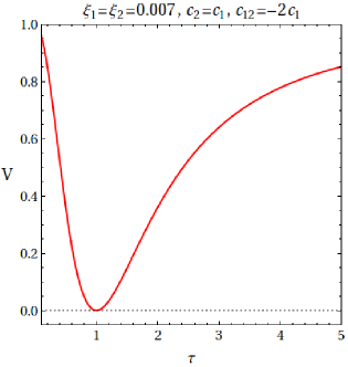
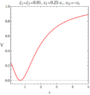
Figure 1: Inflaton potential (divided by constant $V_{0}$) as a function of $\tau=\tan\theta$, for $\xi_{1}=\xi_{2}$ and ratios $c_{12}/c_{1}$, $c_{2}/c_{1}$ of values shown above. $V=0$ at the minimum; note $\theta=(\chi/v)\sqrt{\xi_{1}/6}$ with $\chi$ the actual inflaton. The spectral index and tensor-to-scalar ratio for these cases are shown in Figure 2.

The slow-roll parameters (for $\xi_{1}=\xi_{2}$) are given by

$$\epsilon = \frac{1}{3}\,\xi_{1}\,\frac{\Big{(}c_{2}-c_{1}+(c_{1}-c_{12}+c_{2})\cos(2\theta)\Big{)}^{2}\sec^{4}\theta\tan^{2}\theta}{(c_{2}+c_{12}\tan^{2}\theta+c_{1}\tan^{4}\theta)^{2}},$$ (55)

$$\eta = -\frac{1}{3}\,\xi_{1}\,\frac{\Big{(}(c_{2}-c_{1})\cos(2\theta)+(c_{1}-c_{12}+c_{2})\cos(4\theta)\Big{)}\sec^{4}\theta}{c_{2}+c_{12}\tan^{2}\theta+c_{1}\tan^{4}\theta}.$$ (56)

We find that $\epsilon$ and $\eta$ can be small simultaneously for $\xi_{1}\ll 1$.

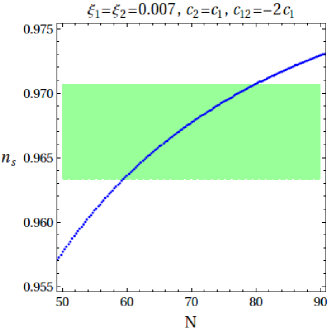
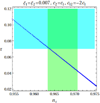
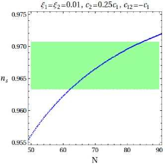
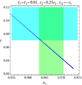
Figure 2: Left: The spectral index $n_{s}$ as a function of the number of e-foldings $N$ for two different cases. Right: The spectral index $n_{s}$ versus tensor-to-scalar ratio $r$ for the corresponding cases. The green region in all the plots corresponds to Planck2018 values for $n_{s}$ within $1\sigma$ (see text). The cyan region with $r>0.07$ is excluded by Planck at 95% CL. We chose $\xi_{1}=\xi_{2}$ for all the plots and $c_{2}/c_{1}=1$ and $c_{12}/c_{1}=(-2)$ (upper panels) and $c_{2}/c_{1}=0.25$ and $c_{12}/c_{1}=(-1)$ (lower panels). Here $c_{12}$ is fixed by the condition ${\hat{V}}=0$ at the minimum.

If we choose $c_{2}=c_{1}$, $c_{12}=-2c_{1}$ then the expressions of the slow-roll parameters simplify further:

$$\epsilon = \frac{4}{3}\,\xi_{1}\tan^{2}(2\theta),$$ (57)

$$\eta = \frac{4}{3}\,\xi_{1}\Big{(}-1+\tan^{2}(2\theta)\Big{)},$$ (58)

which leads to the scalar spectral index and the tensor-to-scalar ratio as

$$n_{s} = 1+2\,\eta_{*}-6\epsilon_{*}=1-\frac{8}{3}\xi_{1}\Big{(}1+2\tan^{2}(2\theta_{*})\Big{)},$$ (59)

and

$$r = 16\,\epsilon_{*}=\frac{64}{3}\,\xi_{1}\tan^{2}(2\theta_{*}).$$ (60)

Further, the number of e-foldings during inflation is also given by

$$N = \,v^{-1}\int^{\chi_{*}}_{\chi_{\rm end}}\frac{{\rm sign}({\hat{V}}^{\prime})d\chi}{\sqrt{2\epsilon(\chi)}}$$ (61)

$$= \frac{3}{4\xi_{1}}\,\log\bigg{|}\frac{\sin(2\theta_{\rm end})}{\sin(2\theta_{*})}\bigg{|}$$

where $\theta_{*}$ is evaluated at the horizon exit and $\theta_{\rm end}$ is the inflaton value at the end of inflation. Inflation ends at $\epsilon=1$, i.e. $|\tan(2\theta_{\rm end})|=(\frac{3}{4\xi_{1}})^{1/2}$ from eq. (57).

The normalization of the CMB anisotropies, $V_{0}/(24\pi^{2}v^{4}\,\epsilon_{*})=2.1\times 10^{-9}$ [45], constrains $c_{1}$ (or equivalently the quartic coupling $\lambda_{1}$) and the non-minimal couplings $\xi_{1,2}$ to satisfy

$$\frac{c_{1}(1+\xi_{1})^{2}}{\xi_{1}^{3}}=1.8\times 10^{-8}\tan^{2}(2\theta_{*}).$$ (62)

This constraint is respected by choosing small values of $c_{1}$ (or $\lambda_{1}$), for given $\xi_{1}$.

We have that $n_{s}=0.9670\pm 0.0039$ ($68\%$ CL) and $r<0.07$ ($95\%$ C.L.) from Planck 2018 (TT, TE, EE + low E + lensing + BK14 + BAO) [45]. In Figure 2, we illustrated the relation between the spectral index versus the number of e-foldings in the left plots and showed the spectral index versus the tensor-to-scalar ratio in the right plots. Here we have fixed $\xi_{1}=\xi_{2}=0.007$, $c_{2}=c_{1}$ and $c_{12}=-2c_{1}$ in the upper panel, and $\xi_{1}=\xi_{2}=0.01$, $c_{2}=0.25c_{1}$, $c_{12}=-c_{1}$ in the lower panel. As a result, we find that our model of inflation is consistent with the observed spectral index and the bound on $r$, for small non-minimal couplings.

5 Conclusions

In this work we discussed the Weyl conformal symmetry and its spontaneous breaking and some implications for model building beyond the SM and inflation.

In models with conformal symmetry (of the Brans-Dicke-Jordan type) with scalar fields with non-minimal couplings to the Ricci scalar, one can generate spontaneously the Planck scale from the vev of a scalar field (or a combination of them). However, a positive (negative) Newton constant is accompanied by a negative (positive) kinetic term for this field, respectively. This situation is naturally avoided in models with an additional Weyl gauge symmetry and a gauge field $\omega_{\mu}$ which is of geometric origin, with a gauge transformation dictated by the conformal transformation of the metric.

We showed that the Weyl field $\omega_{\mu}$ couples only to the scalar sector but not to the fermionic sector of a SM-like Lagrangian in curved space-time, which is interesting for model building. Further, the field $\omega_{\mu}$ undergoes a Stueckelberg mechanism and becomes massive after “eating” the radial mode $\rho\sim\sqrt{K}$ (in field space) and would-be-Goldstone mode (dilaton). The Weyl gauge symmetry is then spontaneously broken (and there are no negative kinetic terms in the theory). Further, the vev $\langle\rho\rangle$ determines the mass of $\omega_{\mu}$ and the Planck scale $M_{p}$ (up to possible additional angular-variables field dependence). The mass of $\omega_{\mu}$ can be larger or smaller than $M_{p}$ depending on the scalar fields charge and non-minimal couplings. After decoupling of $\omega_{\mu}$ the potential depends on the angular variables fields only which can play the role of the neutral Higgs field, inflaton, etc. For two scalar fields of equal non-minimal couplings, the field $\omega_{\mu}$ decouples from the action even if it is light.

For the case with two scalar fields, the scalar potential generally depends only on the angular variable field $\theta$, and it is nearly constant at large $\tan\theta$, when $\omega_{\mu}$ also decouples. Therefore, the potential can be relevant for a single-field inflation. Investigating the details of the inflaton potential, we found that successful inflation is possible, with values of $n_{s}$ and $r$ consistent with Planck2018 constraints, for perturbative values of the couplings.

While this study was formulated in (pseudo)Riemannian geometry extended with a real Weyl field (undergoing a gauge transformation dictated by conformal transformation of the metric), the natural framework is that of Weyl conformal geometry where this symmetry is manifest. In the Riemannian case imposing this symmetry avoids the ghost kinetic term of conformal theory and leads to a Lagrangian with a current $\partial_{\mu}K$ that interacts with the Weyl field. This Lagrangian was shown to be identical, up to a total derivative term, to that obtained in Weyl geometry (WG) where the Weyl symmetric Lagrangian is naturally built-in, with curvature scalar, tensors and affine connection of Weyl geometry. This equivalence is showed for a SM-like Lagrangian endowed with Weyl gauge symmetry, using the relation between $R$ computed in Riemann geometry with Levi-Civita connection and its counterpart in Weyl geometry. This Lagrangian can be used for examining the phenomenological constraints on the SM extended with Weyl gauge symmetry.

Acknowledgements:     The authors are grateful for hospitality and support to CERN Theory Division where this work was done. The work of H.M.L. is supported in part by Basic Science Research Program through the National Research Foundation of Korea (NRF) funded by the Ministry of Education, Science and Technology (NRF-2016R1A2B4008759 and NRF-2018R1A4A1025334). D.M.G. is supported by National Programme PN 18090101.

References

- [1] W. A. Bardeen, “On naturalness in the standard model,” FERMILAB-CONF-95-391-T.
- [2] F. Englert, C. Truffin and R. Gastmans, “Conformal Invariance in Quantum Gravity,” Nucl. Phys. B 117 (1976) 407. doi:10.1016/0550-3213(76)90406-5
- [3] M. Shaposhnikov and D. Zenhausern, “Quantum scale invariance, cosmological constant and hierarchy problem,” Phys. Lett. B 671 (2009) 162 doi:10.1016/j.physletb.2008.11.041 [arXiv:0809.3406 [hep-th]].
- [4] R. Armillis, A. Monin and M. Shaposhnikov, “Spontaneously Broken Conformal Symmetry: Dealing with the Trace Anomaly,” JHEP 1310 (2013) 030 doi:10.1007/JHEP10(2013)030 [arXiv:1302.5619 [hep-th]].
- [5] F. Gretsch and A. Monin, “Perturbative conformal symmetry and dilaton,” Phys. Rev. D 92 (2015) no.4, 045036 doi:10.1103/PhysRevD.92.045036 [arXiv:1308.3863 [hep-th]].
- [6] D. M. Ghilencea, “Quantum implications of a scale invariant regularization,” Phys. Rev. D 97 (2018) no.7, 075015 doi:10.1103/PhysRevD.97.075015 [arXiv:1712.06024 [hep-th]]. D. M. Ghilencea, “Manifestly scale-invariant regularization and quantum effective operators,” Phys. Rev. D 93 (2016) no.10, 105006 doi:10.1103/PhysRevD.93.105006 [arXiv:1508.00595 [hep-ph]]. D. M. Ghilencea, Z. Lalak, P. Olszewski, “Two-loop scale-invariant scalar potential and quantum effective operators,” Eur. Phys. J. C 76 (2016) no.12, 656 doi:10.1140/epjc/s10052-016-4475-0 [arXiv:1608.05336 [hep-th]].
- [7] C. Tamarit, “Running couplings with a vanishing scale anomaly,” JHEP 1312 (2013) 098 doi:10.1007/JHEP12(2013)098 [arXiv:1309.0913 [hep-th]].
- [8] P. G. Ferreira, C. T. Hill and G. G. Ross, “Scale-Independent Inflation and Hierarchy Generation,” Phys. Lett. B 763 (2016) 174 doi:10.1016/j.physletb.2016.10.036 [arXiv:1603.05983 [hep-th]].
- [9] R. Foot, A. Kobakhidze, K. L. McDonald and R. R. Volkas, “Poincaré protection for a natural electroweak scale,” Phys. Rev. D 89 (2014) no.11, 115018 doi:10.1103/PhysRevD.89.115018 [arXiv:1310.0223 [hep-ph]].
- [10] D. M. Ghilencea, Z. Lalak and P. Olszewski, “Standard Model with spontaneously broken quantum scale invariance,” Phys. Rev. D 96 (2017) no.5, 055034 doi:10.1103/PhysRevD.96.055034 [arXiv:1612.09120 [hep-ph]].
- [11] K. Allison, C. T. Hill and G. G. Ross, “Ultra-weak sector, Higgs boson mass, and the dilaton,” Phys. Lett. B 738 (2014) 191 doi:10.1016/j.physletb.2014.09.041 [arXiv:1404.6268 [hep-ph]].
- [12] E. J. Chun, S. Jung and H. M. Lee, “Radiative generation of the Higgs potential,” Phys. Lett. B 725 (2013) 158 Erratum: [Phys. Lett. B 730 (2014) 357] doi:10.1016/j.physletb.2013.11.016, 10.1016/j.physletb.2013.06.055 [arXiv:1304.5815 [hep-ph]].
- [13] C. Brans and R. H. Dicke, “Mach’s principle and a relativistic theory of gravitation,” Phys. Rev. 124 (1961) 925. doi:10.1103/PhysRev.124.925 R. H. Dicke, “Mach’s principle and invariance under transformation of units,” Phys. Rev. 125 (1962) 2163. doi:10.1103/PhysRev.125.2163 P. Jordan, “Schwerkraft und Weltall” 1952. Braunschweig: Vieweg. 2nd revised edition 1955.
- [14] H. Weyl, Gravitation und elektrizität, Sitzungsberichte der Königlich Preussischen Akademie der Wissenschaften zu Berlin (1918), pp.465-480. For a recent review and references see [16].
- [15] P. A. M. Dirac, “Long range forces and broken symmetries,” Proc. Roy. Soc. Lond. A 333 (1973) 403. doi:10.1098/rspa.1973.0070
- [16] E. Scholz, “Weyl geometry in late 20th century physics,” arXiv:1111.3220 [math.HO]; “The unexpected resurgence of Weyl geometry in late 20-th century physics,” Einstein Stud. 14 (2018) 261 doi:10.1007/978-1-4939-7708-611 [arXiv:1703.03187 [math.HO]]. “Paving the Way for Transitions—A Case for Weyl Geometry,” Einstein Stud. 13 (2017) 171 doi:10.1007/978-1-4939-3210-86 [arXiv:1206.1559 [gr-qc]];
- [17] E. Scholz, “Higgs and gravitational scalar fields together induce Weyl gauge,” Gen. Rel. Grav. 47 (2015) no.2, 7 doi:10.1007/s10714-015-1854-z [arXiv:1407.6811 [gr-qc]].
- [18] I. Bars, P. Steinhardt, N. Turok, “Local Conformal Symmetry in Physics and Cosmology,” Phys. Rev. D 89 (2014) no.4, 043515 doi:10.1103/PhysRevD.89.043515 [arXiv:1307.1848 [hep-th]].
- [19] L. Smolin, “Towards a Theory of Space-Time Structure at Very Short Distances,” Nucl. Phys. B 160 (1979) 253. doi:10.1016/0550-3213(79)90059-2
- [20] H. Cheng, “The Possible Existence of Weyl’s Vector Meson,” Phys. Rev. Lett. 61 (1988) 2182. doi:10.1103/PhysRevLett.61.2182
- [21] H. Nishino and S. Rajpoot, “Implication of Compensator Field and Local Scale Invariance in the Standard Model,” Phys. Rev. D 79 (2009) 125025 doi:10.1103/PhysRevD.79.125025 [arXiv:0906.4778 [hep-th]].
- [22] M. de Cesare, J. W. Moffat and M. Sakellariadou, “Local conformal symmetry in non-Riemannian geometry and the origin of physical scales,” Eur. Phys. J. C 77 (2017) no.9, 605 doi:10.1140/epjc/s10052-017-5183-0 [arXiv:1612.08066 [hep-th]].
- [23] H. C. Ohanian, “Weyl gauge-vector and complex dilaton scalar for conformal symmetry and its breaking,” Gen. Rel. Grav. 48 (2016) no.3, 25 doi:10.1007/s10714-016-2023-8 [arXiv:1502.00020 [gr-qc]].
- [24] Y. Tang and Y. L. Wu, “Inflation in gauge theory of gravity with local scaling symmetry and quantum induced symmetry breaking,” Physics Letters B 784 (2018) 163 doi:10.1016/j.physletb.2018.07.048 [arXiv:1805.08507 [gr-qc]].
- [25] A. Davidson and T. Ygael, “Frozen up Dilaton and the GUT/Planck Mass Ratio,” Phys. Lett. B 772 (2017) 5 doi:10.1016/j.physletb.2017.06.001 [arXiv:1706.00368 [gr-qc]].
- [26] J. W. Moffat, “Scalar-tensor-vector gravity theory,” JCAP 0603 (2006) 004 doi:10.1088/1475-7516/2006/03/004 [gr-qc/0506021].
- [27] L. Heisenberg, “Scalar-Vector-Tensor Gravity Theories,” arXiv:1801.01523 [gr-qc].
- [28] J. T. Wheeler, “Weyl geometry,” Gen. Rel. Grav. 50 (2018) no.7, 80 doi:10.1007/s10714-018-2401-5 [arXiv:1801.03178 [gr-qc]].
- [29] I. Quiros, “Scale invariant theory of gravity and the standard model of particles,” arXiv:1401.2643 [gr-qc].
- [30] P. G. Ferreira, C. T. Hill and G. G. Ross, “No fifth force in a scale invariant universe,” Phys. Rev. D 95 (2017) no.6, 064038 doi:10.1103/PhysRevD.95.064038 [arXiv:1612.03157 [gr-qc]].
- [31] P. G. Ferreira, C. T. Hill and G. G. Ross, “Weyl Current, Scale-Invariant Inflation and Planck Scale Generation,” Phys. Rev. D 95 (2017) no.4, 043507 doi:10.1103/PhysRevD.95.043507 [arXiv:1610.09243 [hep-th]].
- [32] P. G. Ferreira, C. T. Hill and G. G. Ross, “Inertial Spontaneous Symmetry Breaking and Quantum Scale Invariance,” arXiv:1801.07676 [hep-th]. C. T. Hill, “Inertial Symmetry Breaking,” arXiv:1803.06994 [hep-th].
- [33] B. Holdom, “Two U(1)’s and Epsilon Charge Shifts,” Physics Letters 166B (1986) 196. doi:10.1016/0370-2693(86)91377-8
- [34] D. M. Ghilencea, “Spontaneous breaking of Weyl quadratic gravity to Einstein action and Higgs potential,” JHEP 1903 (2019) 049 [arXiv:1812.08613 [hep-th]].
- [35] D. M. Ghilencea, “Stueckelberg breaking of Weyl conformal geometry and applications to gravity,” arXiv:1904.06596 [hep-th].
- [36] J. Garcia-Bellido, J. Rubio, M. Shaposhnikov and D. Zenhausern, “Higgs-Dilaton Cosmology: From the Early to the Late Universe,” Phys. Rev. D 84 (2011) 123504 doi:10.1103/PhysRevD.84.123504 [arXiv:1107.2163 [hep-ph]].
- [37] G. K. Karananas and J. Rubio, “On the geometrical interpretation of scale-invariant models of inflation,” Phys. Lett. B 761 (2016) 223 doi:10.1016/j.physletb.2016.08.037 [arXiv:1606.08848 [hep-ph]].
- [38] S. Casas, M. Pauly and J. Rubio, “Higgs-dilaton cosmology: An inflation–dark-energy connection and forecasts for future galaxy surveys,” Phys. Rev. D 97 (2018) no.4, 043520 doi:10.1103/PhysRevD.97.043520 [arXiv:1712.04956 [astro-ph.CO]].
- [39] K. Sravan Kumar and P. Vargas Moniz, “Conformal GUT inflation, proton lifetime and non-thermal leptogenesis,” arXiv:1806.09032 [hep-ph].
- [40] A. S. Koshelev, K. Sravan Kumar and P. Vargas Moniz, “Effective models of inflation from a nonlocal framework,” Phys. Rev. D 96 (2017) no.10, 103503 doi:10.1103/PhysRevD.96.103503 [arXiv:1604.01440 [hep-th]].
- [41] F. Bezrukov, G K. Karananas, J. Rubio and M. Shaposhnikov, “Higgs-Dilaton Cosmology: an effective field theory approach,” Physical Review D 87 (2013) no.9, 096001 doi:10.1103/PhysRevD.87.096001 [arXiv:1212.4148 [hep-ph]].
- [42] T. Banks, M. Johnson and A. Shomer, “A Note on Gauge Theories Coupled to Gravity,” JHEP 0609 (2006) 049 doi:10.1088/1126-6708/2006/09/049 [hep-th/0606277].
- [43] O. Lebedev and H. M. Lee, “Higgs Portal Inflation,” Eur. Phys. J. C 71 (2011) 1821 doi:10.1140/epjc/s10052-011-1821-0 [arXiv:1105.2284 [hep-ph]].
- [44] L. Boubekeur and D. H. Lyth, “Hilltop inflation,” JCAP 0507 (2005) 010 doi:10.1088/1475-7516/2005/07/010 [hep-ph/0502047].
- [45] Y. Akrami et al. [Planck Collaboration], “Planck 2018 results. X. Constraints on inflation,” arXiv:1807.06211 [astro-ph.CO].