Numerical Aspects for Approximating Governing Equations Using Data

Abstract

We present effective numerical algorithms for locally recovering unknown governing differential equations from measurement data. We employ a set of standard basis functions, e.g., polynomials, to approximate the governing equation with high accuracy. Upon recasting the problem into a function approximation problem, we discuss several important aspects for accurate approximation. Most notably, we discuss the importance of using a large number of short bursts of trajectory data, rather than using data from a single long trajectory. Several options for the numerical algorithms to perform accurate approximation are then presented, along with an error estimate of the final equation approximation. We then present an extensive set of numerical examples of both linear and nonlinear systems to demonstrate the properties and effectiveness of our equation recovery algorithms.

1 Introduction

Recently there has been a growing interest in discovering governing equations of certain physical problems using observational data. It is a result of the wide recognition that all physical laws, e.g., Newton’s law, Kepler’s law, etc., were established based on empirical observational data. Since all models and physical laws are approximations to the true physics, a numerically constructed law or governing equation, which albeit may not possess a concise analytical form, could serve as a good model, so long as it is reasonably accurate.

Early work in this direction includes [3, 35], where symbolic regression was used to select physical laws and determine the structure of the underlying dynamical system. More recently, a sparsity-promoting method [7] was proposed to discover governing equations from noisy measurement data. It was based on a sparse regression method ([41]) and a Pareto analysis to construct parsimonious governing equations from a combinatorially large set of candidate models. This methodology was further applied to recovering partial differential equations [31, 34], as well as inferring structures of network models [25]. Conditions were provided in [42] for recovering the governing equations from possibly highly corrupted measurement data, along with a sparse convex optimization method to recover the coefficients of the underlying equations in the space of multivariate polynomials. A nonconvex sparse regression approach was proposed in [32] for selection and identification of a dynamical system directly from noisy data. A model selection approach was developed in [26] for dynamical systems via sparse regression and information criteria. Combining delay embedding and Koopman theory, a data-driven method was designed in [6] to decompose chaotic systems as an intermittently forced linear system. Very recently, three sampling strategies were developed in [33] for learning quadratic high-dimensional differential equations from under-sampled data. There are other techniques that address various aspects of dynamical system discovery problem. These include, but are not limited to, methods to reconstruct the equations of motion from a data series [12], artificial neural networks [19], nonlinear regression [43], equation-free modeling [21], normal form identification [24], empirical dynamic modeling [40, 48], nonlinear Laplacian spectral analysis [18], modeling emergent behavior [30], and automated inference of dynamics [36, 14, 15]. The readers are also referred to the introduction in [5].

The focus of this paper is on the study of local recovery/approximation of general first-order nonlinear ordinary differential/algebraic equations from the time-varying measurement data. The major new features of the proposed numerical framework include the following. First, our method seeks “accurate approximation” to the underlying governing equations. This is different from many of the existing studies, where “exact recovery” of the equations is the goal. The justification for “approximation”, rather than “recovery”, is that all governing equations will eventually be discretized and approximated by certain numerical schemes during implementation. As far as computations are concerned, all numerical simulations are conducted using “approximated” equations. Therefore, as long as the errors in the equation approximation/recovery step is small, comparable to the discretization errors, the approximated equations can be used as sufficient model for simulations. By relaxing the requirement from “exact recovery” to “accurate approximation”, we are able to utilize many standard approximation methods using standard basis functions such as polynomials, which are used in this paper. Consequently, one does not need to choose a (combinatorially) large dictionary in order to include all possible terms in the equations. Since most of the governing equations we encounter in practice have relatively simple and smooth forms, polynomial approximation can be highly accurate at moderately low degrees. Secondly, we propose the use of multiple, in fact a large number of, trajectory data of very short span, instead of using a single long trajectory data as in many existing studies. The length of each burst of the trajectory can be exceptionally short – it needs to be merely long enough to enable accurate estimate of the time derivatives. For noiseless trajectories, the length can as little as 2, for first-order estimation of the time derivative, or 3 for second-order estimation, and so on. We do require that the number of such short bursts of trajectories to be large so that they provide “good” samples in the domain of interest. Upon doing so, we convert the equation recovery problem into a function approximation problem with over-sampled data. A large number of well established approximation algorithms can then be employed. (The readers are referred to earlier books such as [11, 16, 27, 29] for the classical results and methods in function approximation theory.) In this paper, we discuss the results obtained by using least squares method, which is one of the most established methods; $\ell_{1}$ regression method, which is capable of removing data corruption ([9, 38]); and a matrix-free sequential algorithm ([39, 45, 46]), which is suitable for extraordinarily large data sets or stream data. We remark that the use of a very lagre number of trajectory bursts does not necessarily induce large simulation cost, as each burst is of very short length. In fact, in many cases the total amount of data in the large number of bursts is less than that in a single long trajectory. We also remark that the idea of using multiple bursts of trajectories has also be discussed in [33]. The major difference between [33] and this work is that the goal in [33] is for exact recovery of the equation of quadratic form. The bursts are random selected based on the theory of sparse recovery (compressed sensing). In this paper, the bursts are selected using approximation theory, as we only seek to approximate the equations and not recover them. And the equations can be of arbitrary form, beyond polynomials and including algebraic constraints. The choices of the bursts can be random or deterministic, as long as they enable one to obtain accurate approximation.

This paper is organized as follows. After the basis problem setup in Section 2, we present the main method in Section 3, which includes the general formulation, basis selections, trajectory selections, choices of approximation algorithms, and an error bound. We then present, in Section 4, an extensive set of numerical examples, covering a wide variety of linear/nonlinear differential/algebraic equations, to demonstrate the effectiveness of the proposed algorithms.

2 Problem Setup

We consider an autonomous system in the form of

$$\dfrac{d{\bf u}(t)}{dt}={\bf f}({\bf u}),\qquad{\bf u}(t_{0})={\bf u}_{0},$$ (1)

where ${\bf u}=(u_{1},u_{2},\cdots,u_{d})^{\top}$, $d\geq 1$, are state variables, $t_{0}$ the initial time, and ${\bf f}$ defines the evolution of the states. Throughout this paper we call ${\bf u}(t;{\bf u}_{0})$ a trajectory, whose dependence on the initial state ${\bf u}_{0}$ is explicitly shown. The right-hand-side ${\bf f}$ is the “true” and unknown dynamics. Our goal is to construct an accurate representation of ${\bf f}$ using measurement data of the state variables ${\bf u}$.

2.1 Domain-of-Interest

While the state variables ${\bf u}$ may reside in the entire space ${\mathbb{R}}^{d}$, we restrict our equation recovery to a bounded domain $D\subset{\mathbb{R}}^{d}$. We refer to $D$ as the domain-of-interest, which stands for the range of the state variables where one focuses on the underlying problem. Depending on the (unknown) dynamical system and one’s interest in studying it, the definition of the domain-of-interest varies.

Let

$$U_{i}=\left[u_{\min,i},u_{\max,i}\right],\qquad 1\leq i\leq d,$$ (2)

be a closed interval and represent a range of the state variable $u_{i}$, $1\leq i\leq d$, where one wishes to understand the behavior of the system. We then define $D$ as the product of these intervals, i.e.,

$$D=\times_{i=1}^{d}U_{i}.$$ (3)

Effectively this creates a hypercube in $d$ dimensions. We then equip it with a measure $\omega$, which is absolutely continuous and (without loss of generality) satisfies $\int_{D}d\omega=1$. We then invoke the standard definition of inner product

$$\left(g,h\right)_{L^{2}_{\omega}}:=\int_{D}g({\bf x})h({\bf x})d\omega({\bf x}),$$

and its induced norm $\|\cdot\|_{L^{2}_{\omega}}$.

Remark 1

Upon defining the domain-of-interest, we have restricted our equation recovery effort to a “local” manner. This is because recovering the equation in the entire space ${\mathbb{R}}^{d}$, albeit desirable, may be highly challenging, when the underlying dynamical system exhibits complex behaviors that are different in different parts of the space. The use of the domain-of-interest allows one to focus on a region of the domain where the problem can be well behaved and ${\bf f}$ possesses a regular/smooth form, which would be highly advantageous for the recovery effort. The size of $D$ depends on the underlying problem and is not necessarily small.

2.2 Data

Let $t_{0}<t_{1}<\cdots$ be a sequence of time instances. We assume that the true state variables ${\bf u}$ can be observed on these time instances and denote

$${\bf x}(t_{j};{\bf u}_{0})={\bf u}(t_{j};{\bf u}_{0})+{\bm{\epsilon}}_{j},\quad j=0,1,\dots,$$

the observed data for the state trajectory, where ${\bm{\epsilon}}_{j}$ stands for observation errors. The trajectory data can be from different sequences of trajectories, which are originated by different initial states. Let ${\bf u}_{0}^{(1)},\dots,{\bf u}_{0}^{(M)}$, $M\geq 1$, be a set of different initial states. We use the following shorthanded notation to denote the trajectory data from the $m$-th initial condition,

$${\bf x}^{(m)}(t_{j})={\bf u}(t_{j};{\bf u}_{0}^{(m)})+{\bm{\epsilon}}_{j}^{(m)}\in D,\qquad 0\leq j\leq J_{m},\quad 1\leq m\leq M,$$ (4)

where $J_{m}$ is the number of intervals in the $m$-th trajectory data. The collection of all these data shall be used to estimate the true state equation.

2.3 Extension to Differential-Algebraic Equations

It is worth noting that the method discussed in this paper is applicable to semi-explicit differential algebraic equations (DAEs), i.e., DAEs with index 1, in the following form,

$$\dfrac{d{\bf u}(t)}{dt}={{\bf F}}({\bf u},{\bf v}),$$ (5a)

$${{\bf G}}({\bf u},{\bf v})=0,$$ (5b)

where ${\bf u}$ and ${\bf v}$ are the state variables and ${\bf G}$ represents algebraic constraints. Let us assume that the implicit function theorem holds such that the constraint (5b) induces the following explicit relation

$${\bf v}={\bf g}({\bf u}).$$ (6)

Then, by letting ${\bf f}({\bf u})={{\bf F}}({\bf u},{\bf g}({\bf u}))$, the DAEs can be written in the same form as the autonomous system (1).

3 Main Numerical Algorithm

In this section we discuss numerical aspects of our equation approximation/recovery method. We first present the general formulation, which is rather similar to many of the existing work (e.g., [3, 7, 32]). The details of the numerical algorithm, which is different and new, are then presented, along with an error analysis.

3.1 General Formulation

Let $\{\mathbf{x}\}$ be a collection of trajectory data, in the form of (4). We assume that the time derivatives of the trajectory are also available at some time instances $t_{j},j\in\Theta_{m}\subseteq\{0,1,\cdots,J_{m}\}$, either produced by the measurement procedure or approximated numerically using $\{\mathbf{x}\}$. Let

$${\bf{\dot{x}}}(t)={\bf{\dot{u}}}(t)+\bm{\tau}(t),$$

be the derivative data, where $\bm{\tau}(t)$ stands for the errors or noises. This creates a set of data pairings at the time instances $\{t_{j},j\in\Theta_{m}\}$, where both the state variables and their derivatives are available. The collection of such pairings are denoted as

$$\left\{{\bf x}^{(m)}(t_{j}),\dot{\bf x}^{(m)}(t_{j})\right\},\qquad j\in\Theta_{m},\quad 1\leq m\leq M,$$ (7)

where the total number of data pairings is

$$M_{tot}=\sum_{m=1}^{M}\#\Theta_{m}.$$

We then choose a (large) set of dictionary $\Phi=\{\phi_{1},\dots,\phi_{N}\}$ to represent ${\bf f}$ in the governing equation (1). For the vector function ${\bf f}=(f_{1},\dots f_{d})$, its approximation is typically conducted component-wise. That is, for each $\ell=1,\dots,d$, we seek

$$f_{\ell}(\mathbf{x})\approx\tilde{f}_{\ell}(\mathbf{x}):=\sum_{j=1}^{N}c_{j,\ell}\phi_{j}(\mathbf{x}).$$ (8)

Here the functions $\{\phi_{j}(\mathbf{x})\}$ in the dictionary should contain all the possible functions one wishes to incorporate, for the accurate approximation of ${\bf f}$. Some examples are

$$\Phi=\{{\bf 1},\mathbf{x},\mathbf{x}^{2},\dots,\mathbf{x}^{n},\sin\mathbf{x},\cos\mathbf{x},\dots,\sin m\mathbf{x},\cos m\mathbf{x},\exp(\pm\mathbf{x}),\dots,\exp(\pm k\mathbf{x}),\dots\}.$$ (9)

Let $\mathbf{A}$ be a $(M_{tot}\times N)$ model matrix

$$\mathbf{A}=(a_{ij}),\qquad a_{ij}=\phi_{j}(\mathbf{x}_{i}),\qquad 1\leq i\leq M_{tot},\quad 1\leq j\leq N,$$

where $(\mathbf{x}_{i},{\dot{\mathbf{x}}}_{i})$ represents the $i$-th data pairing in (7). The equation recovery problem is then cast into an approximation problem

$$\mathbf{Ac}_{\ell}\approx\dot{\mathbf{X}}_{\ell},\qquad\ell=1,\dots,d,$$ (10)

where $\dot{\mathbf{X}}_{\ell}$ is the vector of $\ell$-th component of all available derivatives in the pairings (7), and $\mathbf{c}_{\ell}=(c_{1,\ell}\dots,c_{N,\ell})^{T}$ is the coefficient vector to be solved.

Once an accurate approximation is obtained, we consider

$${}\dfrac{d{\bf x}(t)}{dt}=\tilde{\bf f}({\bf x}),$$ (11)

as an approximation of the true system (1).

It should be noted that converting the equation recovery problem into an approximation problem in the form of (10) is a rather standard framework in the existing studies. In most of the existing studies, one typically chooses the dictionary (9) to be very large (often combinatorially large) and then use a certain sparsity-promoting method to construct a parsimonious solution, e.g., $\ell_{1}$ minimization for underdetermined system. By doing so, if the terms in the true equations are already included in the dictionary (9), it is then possible to exactly recover the form of the governing equations.

Hereafter, we will present the detail of our numerical approach, which is different from most of the existing approaches.

3.2 Equation Approximation using Standard Basis

Contrary to most of the existing studies, our method here does not utilize a combinatorially large dictionary to include all possible terms in the equations. Instead, we propose to use a “standard” set of basis functions, particularly polynomials in term of $\mathbf{x}$, to approximate ${\bf f}$ directly. One certainly is not restricted to polynomials and can use other basis such as radial basis functions. Here we choose polynomials merely because it is one of the most widely used basis for function approximation. By doing so, we give up the idea of “exact recovery” of ${\bf f}$, as exact recovery is not possible unless the true governing equations are strictly of polynomial form (which in fact is not uncommon). Instead, our approach focuses on obtaining an approximation of ${\bf f}$ with sufficiently high accuracy. We remark that this is satisfactory for practical computations, as the exact governing equations (even if known) are often discretized and approximated by a certain numerical scheme after all. So long as the errors in the equation recovery/approximation step is sufficiently small, compared to the discretization errors, the approximated governing equations can be as effective as the true model. Even though our method will not recover the true equations exactly in most cases, we shall continue to loosely use the term “equation recovery” hereafter, interchangeable with “equation approximation”.

To construct the approximation $\tilde{\bf f}$, we confine ourself to a finite dimensional polynomial space $V\subset L^{2}_{\omega}(D)$ with $\dim V=N\geq 1$. Without loss of generality, we take $d\omega=\frac{1}{\int_{D}d{\bf x}}d{\bf x}$, and let the subspace $V$ be $\Pi_{n}^{d}$, the linear subspace of polynomials of degree up to $n\geq 1$. That is,

$$\Pi_{n}^{d}=\text{span}\{{\bf x}^{{\bf i}}=x_{1}^{i_{1}}\cdots x_{d}^{i_{d}},|{\bf i}|\leq n\},$$ (12)

where ${\bf i}=(i_{1},\dots,i_{d})$ is multi-index with $|{\bf i}|=i_{1}+\cdots+i_{d}$. Immediately, we have

$$N=\dim\Pi_{n}^{d}={n+d\choose d}=\frac{(n+d)!}{n!d!}.$$ (13)

Let $\{\phi_{j}({\bf x})\}_{j=1}^{N}$ be a basis of $V$. We then seek an approximation $\tilde{\bf f}\approx{\bf f}$ in a component-wise manner. That is, for the $\ell$-th component, we seek

$$\tilde{f}_{\ell}({\bf x})=\sum_{j=1}^{N}c_{j,\ell}\phi_{j}({\bf x}),\quad\ell=1,\dots,d.$$ (14)

Upon adopting the following vector notations

$${\bf\Phi}({\bf x})=\big{(}\phi_{1}({\bf x}),\cdots,\phi_{N}({\bf x})\big{)}^{\top},\qquad{\bf c}_{\ell}=\big{(}c_{1,\ell},c_{2,\ell},\cdots,c_{N,\ell}\big{)}^{\top},$$ (15)

we write

$$\tilde{f}_{\ell}({\bf x})=\langle{\bf c}_{\ell},{\bf\Phi}({\bf x})\rangle,\qquad\ell=1,\dots,d.$$ (16)

Our goal is to compute the expansion coefficients in ${\bf c}_{\ell}$, $\ell=1,\dots,d$. Later in Section 3.4 we will introduce several algorithms to compute the coefficients ${\bf c}_{\ell}$.

Unless the form of the true system (1) is of polynomial, we shall not obtain exact recovery of the equation. For most physical systems, their governing equations (1) consist of smooth functions, we then expect polynomials to produce highly accurate approximations with low or modest degrees. On the other hand, if one possesses sufficient prior knowledge of the underlying system and is certain that some particular terms should be in the governing equations, then those terms can be incorporated in the dictionary, in addition to the standard polynomial basis.

3.3 Selection of Trajectories

Upon setting the basis for the approximation, it is important to “select” the data. Since the problem is now casted into an approximation problem in $D\subset{\mathbb{R}}^{d}$, many approximation theories can be relied upon. One of the key facts from approximation theory is that, in order to construct accurate function approximation, data should fill up the underlying domain in a systematic manner. This implies that we should enforce the data pairings (7) to “spread” out the domain-of-interest $D$. Since the trajectories of many dynamical systems often evolve on certain low-dimensional manifolds, using a single trajectory, no matter how long it is, will unlikely to produce a set of data pairings for accurate approximation, except for some special underlying systems such as the chaotic systems [42]. This is the reason why we propose to use multiple number of short trajectories. Specifically, the trajectories are started from different initial conditions. The length of each trajectories may be very short — just long enough to allow one to estimate the time derivatives. More specifically, we conduct the following steps.

• Let $M\geq 1$ be the number of trajectories, and

  $$\mathbf{x}^{(m)}_{0}={\bf u}_{0}^{(m)}+{\bm{\epsilon}}_{0}^{(m)},\qquad m=1,\dots,M,$$

  are different initial data, where ${\bm{\epsilon}}_{0}^{(m)}$ is the observation error.

• For each initial state, collect trajectory data generated by the underlying system (1)

  $${\mathbf{x}}^{(m)}(t_{j})={\bf u}(t_{j};{\bf u}_{0}^{(m)})+{\bm{\epsilon}}_{j}^{(m)}\in D,\qquad 0\leq j\leq J_{m},\quad 1\leq m\leq M,$$ (17)

  where $J_{m}$ is the number of data points collected for the $m$-th trajectory and ${\bm{\epsilon}}_{j}^{(m)}$ is the observation noise.

• Collect or estimate the time derivatives of the trajectories by using the data in (17)

  $${\dot{\mathbf{x}}}^{(m)}(t_{j})={\dot{\bf u}}(t_{j};{\bf u}_{0}^{(m)})+\bm{\tau}^{(m)}(t_{j}),\qquad j\in\Theta_{m},\quad 1\leq m\leq M,$$ (18)

  where $\bm{\tau}^{(m)}(t_{j})$ stands for the estimation/observation errors, and $\Theta_{m}=\{j_{1}^{(m)},\cdots,j_{s_{m}}^{(m)}\}\subseteq\{0,\cdots,J_{m}\}$.

• The pairings

  $$\left\{\mathbf{x}^{(m)}(t_{j}),{\dot{\mathbf{x}}}^{(m)}(t_{j})\right\},\qquad j\in\Theta_{m},\quad 1\leq m\leq M,$$ (19)

  are the data we use to approximation the equation, where ${\mathbf{x}}^{(m)}(t_{0})=\mathbf{x}^{(m)}_{0}$ is the initial state.

We propose to use a large number of short bursts of trajectories, i.e.,

$$J_{m}\sim{\mathcal{O}}(1),\quad m=1,\dots,M,\qquad M\gg 1.$$ (20)

The length of each trajectory, $(J_{m}+1)$, is very small – it should be merely long enough to allow accurate estimation of the time derivatives. In case the time derivatives are available by other means, e.g., direct measurement, then $J_{m}$ can be set to 0.

There are several approaches to choose different initial states $\{{\bf u}_{0}^{(m)}\}$ from the region $D$. They include but are not limited to

• Sampling the initial states $\{{\bf u}_{0}^{(m)}\}$ from some random distribution defined on $D$, e.g., the uniform distribution.

• Sampling the initial states $\{{\bf u}_{0}^{(m)}\}$ by quasi-Monte Carlo sequence, such as the Sobol or Halton sequence, or other lattice rules.

• If $D$ is a hypercube, the initial state set $\{{\bf u}_{0}^{(m)}\}$ can be taken as the set of quadrature points (e.g., the Gaussian points) or its random subset [49]. One can also sample the quadrature points according some discrete measure [45].

3.4 Numerical Strategies

We now discuss several key aspects of the numerical implementation of the method.

3.4.1 Computation of time derivatives

In most of the realistic situations, only the trajectory data $\{{\bf x}^{(m)}(t_{j})\}$ are available, and the time derivatives ${\bf\dot{x}}^{(m)}(t_{j})$ need to be approximated numerically. Given a set of trajectory data $\{{\bf x}^{(m)}(t_{j}),0\leq j\leq J_{m}\}$, we seek to numerically estimate the approximate time derivative ${\bf\dot{x}}^{(m)}(t_{j})$ at certain time instances $t_{j}$, $j\in\Theta_{m}\subseteq\{0,\cdots,J_{m}\}$. This topic belongs to the problem of numerical differentiation of discrete data.

If the data samples are noiseless, the velocity can be computed by a high-order finite difference method, e.g., a second-order central approximation with $J_{m}=2$ and $t_{j}=j\Delta t$ is

$${\bf\dot{x}}^{(m)}(t_{1})=\frac{{\bf\dot{x}}^{(m)}(t_{2})-{\bf\dot{x}}^{(m)}(t_{0})}{2\Delta t}.$$ (21)

However, when data contain noise, estimation of derivatives can be challenging. In this case, if one uses the standard finite difference methods, then the resulting noise level in the first derivatives ${\bf\dot{x}}^{(m)}(t_{j})$ scales as $\sim\frac{{\bm{\epsilon}}_{j}^{(m)}}{\Delta t}$. (See [44] for more analysis.) Several approaches were developed for numerical differentiation of noisy data. They include least squares approximation methods [22, 44], Tikhonov regularization [13], total variation regularization [10], Knowles and Wallace variational method [23], etc. For an overview, see [22].

In this paper, we use the least squares approach to denoise the derivative ${\bf\dot{x}}^{(m)}(t_{j})$. The approach consists of constructing a least squares approximation of the trajectory, followed by an analytical differentiation of the approximation to obtain the derivatives. With the $m$-th burst of trajectory data, $m=1,\dots,M$, we first construct a polynomial ${\bf p}(t)=\sum_{k=0}^{L}{\bf a}_{k}\left(t-t_{j}\right)^{k}$ as an approximation to the trajectory ${\bf u}(t;{\bf u}_{0}^{(m)})$, by using the least squares method with $1\leq L\leq J_{m}$. We then estimate the derivative as ${\bf\dot{x}}^{(m)}(t_{j})={\bf a}_{1}$.

We remark that other methods for derivative computation with denoising effect can be certainly used. We found the least squares method to be fairly robust and easy to implement. When the noise level in the data become too large to obtain accurate derivatives, our method would become unreliable. This is, however, a universal challenge for all methods for equation recovery.

We also remark that even though the number of trajectories can be very large, i.e., $M\gg 1$. Since each trajectory is very short with $J_{m}\sim{\mathcal{O}}(1)$, $m=1,\dots,M$, the total amount of data for the state variables scales as $\mathcal{O}(M)$. In many cases this is fairly small.

3.4.2 Recovery algorithms: Regression methods

The regression methods seek the expansion coefficients ${\bf c}_{\ell}$ by solving the following minimization problems

$${\bf c}_{\ell}=\operatornamewithlimits{argmin}_{{\bf c}\in\mathbb{R}^{N}}\|{\bf A}{\bf c}-\dot{\mathbf{X}}_{\ell}\|,\quad\ell=1,\dots,d,$$ (22)

where the norm $\|\cdot\|$ can be taken as the vector $\ell_{2}$-norm $\|\cdot\|_{2}$, which corresponds to the well known least squares method and can handle noisy data. It can also be taken as the vector $\ell_{1}$-norm, which is the least absolute deviation (LAD) method and can eliminate potential corruption errors in data (cf. [9, 38]). If one would like to seek the sparse coefficients ${\bf c}_{\ell}$, the LASSO (least absolute shrinkage and selection operator) method [41] may be used,

$${\bf c}_{\ell}=\operatornamewithlimits{argmin}_{{\bf c}\in\mathbb{R}^{N}}\frac{1}{2}\|{\bf A}{\bf c}-\dot{\mathbf{X}}_{\ell}\|^{2}+\lambda\|{\bf c}\|_{1},\quad\ell=1,\dots,d,$$ (23)

where $\lambda$ is a parameter to be chosen. Since our method here seeks accurate approximation to the governing equations, rather than exact recovery, we focus on the use of least squares and LAD.

Remark 2

The methods discussed here are based on component-wise approximation of the state variable ${\bf u}$. That is, each component of the states is approximated independently. It is possible to seek joint approximation of all components of ${\bf u}$ simultaneously. A joint approximation may offer computational advantages and yet introduce new challenges. We shall leave this to a separate study.

3.4.3 Recovery algorithms: Matrix-free method

When the data set is exceptionally large ($M\gg 1$), or unlimited as in stream data, matrix-free method such as the sequential approximation (SA) method (cf. [39, 45, 46, 37]), can be more effective.

The SA method is of iterative nature. It aims at conducting approximation using only one data point at each step. By starting from arbitrary choices of the initial approximation, which corresponds to an arbitrary choice of the coefficient vectors $\mathbf{c}_{\ell}^{(0)}$ at $k=0$ step, the iteration of the coefficient vector at $k\geq 1$ step is

$${\bf c}_{\ell}^{(k)}={\bf c}_{\ell}^{(k-1)}+\frac{{{\dot{x}}}_{\ell}^{(k)}(t_{j_{k}})-\langle{\bf c}^{(k-1)}_{\ell},{\bf\Phi}({\bf x}^{(k)}(t_{j_{k}}))\rangle}{\left\|{\bf\Phi}({\bf x}^{(k)}(t_{j_{k}}))\right\|_{2}^{2}+\gamma_{k}}{\bf\Phi}({\bf x}^{(k)}(t_{j_{k}})),\quad k=1,\dots,$$ (24)

where $\gamma_{k}\geq 0$ are parameters chosen according to the noise level in the $k$-th piece of data $\big{(}{\bf x}^{(k)}(t_{j_{k}}),{\dot{\bf x}}^{(k)}(t_{j_{k}})\big{)}$, and $\dot{x}_{\ell}$ denotes the $\ell$-th component of $\dot{\bf x}$. For noiseless data, one can set $\gamma_{k}=0$.

The scheme is derived by minimizing a cost function that consists of data mismatch at the current arriving data point and the difference in the polynomial approximation between two consecutive steps. The method is particularly suitable for stream data arriving sequentially in time, as it uses only one data point at each step and does not require storage or knowledge of the entire data set. Moroever, the scheme uses only vector operations and does not involve any matrices. For more details of the method, including convergence and error analysis, see [39, 45, 46, 37].

3.5 Error analysis

Assuming the aforementioned numerical algorithms can construct a sufficiently accurate approximation of ${\bf f}$ with a error bound $\|\tilde{\bf f}-{\bf f}\|_{2,L^{2}_{\omega}}$, we can estimate the error in solution of the recovered system (11).

Let ${\bf x}(t)$ be the exact solution of the recovered system (11) and ${\bf u}(t)$ the exact solutions of true system (1). Assume that ${\bf x}(t_{0})={\bf u}(t_{0})\in D$, we then have the following error bound for the difference between ${\bf x}(t)$ and ${\bf u}(t)$.

Theorem 1

Assume $\bf f$ is Lipschitz continuous on $D$,

$$\|{\bf f}({\bf u}_{1})-{\bf f}({\bf u}_{2})\|_{2}\leq L_{f}\|{\bf u}_{1}-{\bf u}_{2}\|_{2},\quad\forall{\bf u}_{1},{\bf u}_{2}\in D.$$

If ${\bf x}(t),{\bf u}(t)\in D$, for $t_{0}\leq t\leq T$, then

$$\big{\|}{\bf x}(t)-{\bf u}(t)\big{\|}_{2}\leq(t-t_{0})\|\tilde{\bf f}-{\bf f}\|_{2,L^{\infty}}+L_{f}\int_{t_{0}}^{t}\big{\|}{\bf x}(s)-{\bf u}(s)\big{\|}_{2}ds,$$ (25)

Furthermore

$$\big{\|}{\bf x}(t)-{\bf u}(t)\big{\|}_{2}\leq L_{f}^{-1}\big{(}{\rm e}^{L_{f}(t-t_{0})}-1\big{)}\Big{(}\|{\bf f}-{\mathcal{P}}_{V}{\bf f}\|_{2,L^{\infty}}+\|\tilde{\bf f}-{\mathcal{P}}_{V}{\bf f}\|_{2,L^{2}_{\omega}}\|\sqrt{K}\|_{L^{\infty}}\Big{)},$$ (26)

where the operator ${\mathcal{P}}_{V}$ denotes the component-wise projection on to $V$, and $K(\mathbf{x})$ denotes the “diagonal” of the reproducing kernel of $V$. With any orthogonal basis $\{\psi_{j}(\mathbf{x})\}_{j=1}^{N}$ of $V$, the kernel $K$ can be expressed as $K(\mathbf{x})=\sum_{j=1}^{N}\psi_{j}^{2}(\mathbf{x}).$

The proof can be found in A. We remark that the error bound here is rather crude, as it addresses a general system of equation. More refined error bounds can be derived when one has more knowledge of the underlying system of equations.

4 Numerical Examples

In this section we present numerical examples to verify the performance of the proposed methods for recovering the ordinary differential equations (ODEs) and semi-explicit differential algebraic equations (DAEs).

In all the test cases, we assume that there is no prior knowledge about the governing equations. Without loss of generality, we assume that $t_{j}=j\Delta t$. Unless otherwise stated, $\Delta t$ is taken as $0.005$, the initial states $\{{\bf u}_{0}^{(m)}\}$ are sampled by the uniform distribution over the region $D$, and the basis is taken as $\{{\bf x}^{\bf i},|{\bf i}|\leq n\}$. We employ a variety of test cases of both linear and nonlinear systems of ODEs. The examples include relatively simple and well understood ODE systems from the textbook [4], as well as more complex nonlinear systems of coupled ODE and DAEs. Moreover, we also introduce corruption errors in the trajectory data, in addition to the standard random noises. We examine not only the errors in approximating the exact equations, but also the errors in the predictions made by the recovered equations.

Our primary focus is to demonstrate the flexibility of using polynomial approximation for accurate equation approximation, rather than exact recovery, as well as the effect of using a large number of short bursts of trajectories. For the actual computation of the approximation, we primarily use the standard least squares method. When data corruption exists, we also use LAD, i.e., $\ell_{1}$ regression, and employed the software package $\ell_{1}$-Magic [8]. We also include an example with a very large data set and use the sequential method to demonstrate the flexibility of the matrix-free method.

4.1 Linear ODEs

We first present a set of numerical results for simple linear ODEs with $d=2$, to examine the performance of the methods in recovering the structure of ODEs around different types of critical points. All examples are textbook problems from [4].

Example 1

Six linear ODE systems are considered here, and their structures cover all the elementary critical points. The description of the systems and the corresponding numerical results are displayed in Table 1. In all the tests, $n=1$ is used. The first and second tests use $M=10$ sets of noiseless trajectory data. The third and forth tests use $M=10$ sets of noisy trajectory data, where the noise follows uniform distribution in $[-0.01,0.01]$. The last two tests considers $M=20$ sequences of trajectory data, with two uncertain (randomly chosen) sequences ($10\%$ of the total sequences) have large corruption errors following the normal distribution $N(0.5,1)$. It is seen from Table 1 that the proposed methods are able to recover the correct structure of the ODE systems from few measurement data. The values of approximate coefficients in the learned governing equations are very close to the true values.

We now discuss the need for using a large number of short bursts of trajectory data. Let us consider the fourth linear ODE system in Table 1, which is the nodal sink system

$$\begin{cases}\dot{u}_{1}=-2u_{1}+u_{2}-2,\\ \dot{u}_{2}=u_{1}-2u_{2}+1.\end{cases}$$ (27)

Assume that the observed data are from a single trajectory

$${\bf x}(t_{j};{\bf u}_{0})={\bf u}(t_{j};{\bf u}_{0}),$$

originated from the initial state ${\bf u}_{0}$. If ${\bf u}_{0}$ belongs to the line $\Gamma=\{{\bf u}=(u_{1},u_{2}):u_{2}-u_{1}-1=0\}$, then all the data on the trajectory $\{{\bf x}(t_{j};{\bf u}_{0})\}$ belong to $\Gamma$. It is straightforward to see that the solution of the following linear system

$$\begin{cases}\dot{u}_{1}=-u_{2}+\eta_{1}(u_{2}-u_{1}-1),\\ \dot{u}_{2}=-u_{2}+\eta_{2}(u_{2}-u_{1}-1),\end{cases}$$ (28)

can exactly fit the data on $\Gamma$, for arbitrary $\eta_{1},\eta_{2}\in\mathbb{R}$. This implies that recovering (27) becomes an ill-posed problem, as there are infinite number of linear systems (28) that correspond to such a single trajectory data. From the point of view of function approximation, this is not surprising, as a single trajectory of a given system often falls onto a certain low dimensional manifold (unless the system is chaotic). Approximating an unknown function using data from a low-dimensional manifold is highly undesirable and can be ill-posed. The use of a large number of short bursts of trajectory effectively eliminates this potential difficulty.

Table 1: Example 1: Local recovery of linear ODEs

0.16 0.21 0.23 0.20 0.16

Phase portrait True system Computational settings Learned system Learned portrait

Saddle point
$\begin{aligned} &\dot{u}_{1}=u_{1}+u_{2}-2\\ &\dot{u}_{2}=u_{1}-u_{2}\end{aligned}$ $D=[0,2]^{2}$
Noiseless data with $J_{m}=2$
Least squares regression $\begin{aligned} \dot{x}_{1}&=1.0000083x_{1}\\ &\quad+1.0000003x_{2}\\ &\quad 1.0000083\\ \dot{x}_{2}&=1.0000083x_{1}\\ &\quad-1.0000083x_{2}\\ &\quad-1.65\times 10^{-14}\end{aligned}$

Improper node
$\begin{aligned} &\dot{u}_{1}=u_{1}-4u_{2}\\ &\dot{u}_{2}=4u_{1}-7u_{2}\end{aligned}$ $D=[-1,1]^{2}$
Noiseless data with $J_{m}=2$
$\ell_{1}$-regression $\begin{aligned} \dot{x}_{1}&=1.00034x_{1}\\ &\quad-4.00045x_{2}\\ &\quad+4.05\times 10^{-16}\\ \dot{x}_{2}&=4.00045x_{1}\\ &\quad-7.00056x_{2}\\ &\quad+1.50\times 10^{-15}\end{aligned}$

Star point
$\begin{gathered}\dot{u}_{1}=-u_{1}\\ \dot{u}_{2}=-u_{2}\end{gathered}$ $D=[-1,1]^{2}$
Noisy data with $J_{m}=19$
Least squares regression $\begin{aligned} \dot{x}_{1}&=-1.0265x_{1}\\ &\quad+0.0131x_{2}\\ &\quad-0.0146\\ \dot{x}_{2}&=-0.0392x_{1}\\ &\quad-1.000038x_{2}\\ &\quad+0.0036\end{aligned}$

Nodal sink
$\begin{gathered}\dot{u}_{1}=-2u_{1}+u_{2}-2\\ \dot{u}_{2}=u_{1}-2u_{2}+1\\ u_{2}>u_{1}\end{gathered}$ $D=[-2,0]\times[-1,1]\cap\{{\bf x}|x_{2}>x_{1}\}$
Noisy data with $J_{m}=19$
Least squares regression $\begin{aligned} \dot{x}_{1}&=-1.9556x_{1}\\ &\quad 0.9693x_{2}\\ &\quad-1.9638\\ \dot{x}_{2}&=1.0061x_{1}\\ &\quad-1.9920x_{2}\\ &\quad+1.0011\end{aligned}$

Center point
$\begin{aligned} &\dot{u}_{1}=u_{1}+2u_{2}\\ &\dot{u}_{2}=-5u_{1}-u_{2}\end{aligned}$ $D=[-1,1]^{2}$
Corrupted data with $J_{m}=2$
$\ell_{1}$-regression $\begin{aligned} \dot{x}_{1}&=0.9999625x_{1}\\ &\quad+1.999925x_{2}\\ &\quad+6.90\times 10^{-14}\\ \dot{x}_{2}&=-4.9998125x_{1}\\ &\quad-0.9999625x_{2}\\ &\quad-4.10\times 10^{-13}\end{aligned}$

Spiral point
$\begin{gathered}\dot{u}_{1}=-u_{1}-u_{2}-1\\ \dot{u}_{2}=2u_{1}-u_{2}+5\\ (u_{1}+2)^{2}+(u_{2}-1)^{2}\leq 1\end{gathered}$ $D=\{{\bf x}|(x_{1}+2)^{2}+(x_{2}-1)^{2}\leq 1\}$
Corrupted data with $J_{m}=2$
$\ell_{1}$-regression $\begin{aligned} \dot{x}_{1}&=-0.999979x_{1}\\ &\quad-1.000004x_{2}\\ &\quad-0.999954\\ \dot{x}_{2}&=2.0000083x_{1}\\ &\quad-0.99997917x_{2}\\ &\quad+4.9999958\end{aligned}$

4.2 Nonlinear ODEs

We then test the proposed methods for recovering nonlinear ODE systems exhibiting more complex dynamics. In general, the nonlinear ODEs do not have explicit analytical solutions, we therefore generate the measurement data by numerically solving the ODEs using the forth-order explicit Runge-Kutta method with a small time step-size.

Example 2

We first consider the undamped Duffing equation

$$\ddot{u}+u+\epsilon u^{3}=0,$$

where $\epsilon$ is a small positive number and specified as $10^{-4}$. Taking $u_{1}=u$ and $u_{2}=\dot{u}$ gives

$$\begin{cases}\dot{u}_{1}=u_{2},\\ \dot{u}_{2}=-u_{1}-\epsilon u_{1}^{3}.\end{cases}$$ (29)

The region $D$ is specified as $[0,2]\times[-1,1]$. From $M=30$ bursts of noiseless trajectory data with $J_{m}=2$, we try to learn the governing system using different regression methods with $n=3$. The errors of approximate expansion coefficients in the learned systems are displayed in Fig. 1. As we can see, the coefficients are recovered with high accuracy by $\ell_{1}$ and $\ell_{2}$ regressions.

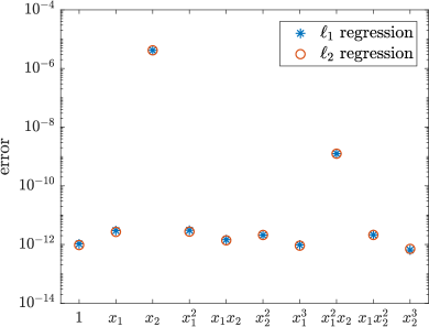
(a) Errors in coefficients $\mathbf{c}_{1}$

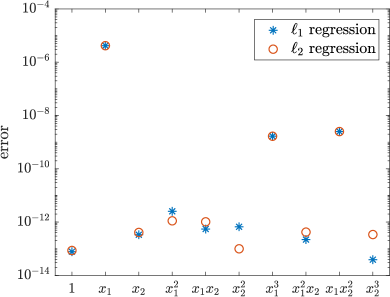
(b) Errors in coefficients $\mathbf{c}_{2}$

Figure 1: Example 2: Results for recovering the system (29). The symbols “$\ast$” and “$\circ$” represent the results of $\ell_{1}$ and $\ell_{2}$ regression methods, respectively. The coefficient errors which are not shown in the figures are zero errors.

Example 3

We consider

$$\begin{cases}\dot{u}_{1}=u_{1}(1-u_{1}-u_{2}),\\ \dot{u}_{2}=u_{2}(0.5-0.25u_{2}-0.75u_{1}),\end{cases}$$ (30)

whose qualitative behavior was studied in [4]. We take $D=[-1,2]\times[-0.5,3]$, which contains the four critical points, an unstable node $(0,0)$, two asymptotically stable nodes $(1,0)$ and $(0,2)$, and a saddle point $(0.5,0.5)$. Suppose we have $M=30$ sets of trajectory data with $J_{m}=30$, and all the data contain i.i.d. random noises following uniform distribution in $[-0.01,0.01]$. Learning from these data, the least squares regression method with $n=2$ produced the following approximate system

$$\begin{cases}\dot{x}_{1}=x_{1}(1.0217-1.0166x_{1}-1.0164x_{2})-0.01695+0.0350x_{2}-0.0128x_{2}^{2},\\ \dot{x}_{2}=x_{2}(0.50914-0.2500x_{2}-0.7544x_{1})-0.0160+0.0086x_{1}-0.0016x_{1}^{2}.\end{cases}$$ (31)

Although in this case the data contain noises at a relatively large level, the proposed method can still recover the coefficients with errors less than $4\times 10^{-2}$. In Figure 2, the phase portraits of the original and recovered systems are plotted to provide a qualitative comparison between the true and the learned dynamics. Good agreements are observed in the structures, and the four critical points are correctly detected. Figure 3 shows the solutions of the original and recovered systems at the initial state $(1.25,1.75)$, as well as the errors in the learned solution.

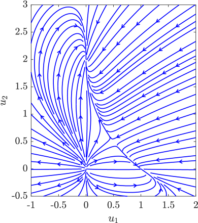
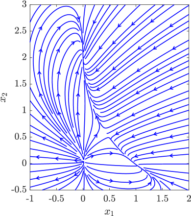
Figure 2: Example 3: Phase portraits for the true system (30) (left) and the learned system (31) (right).

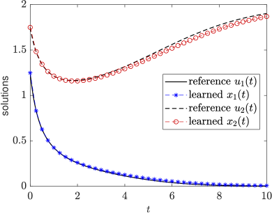
Figure 3: Example 3: Validation of the recovered system (31) with initial state $(1.25,1.75)$. Left: solutions. Right: error $\|{\bf x}(t)-{\bf u}(t)\|_{2}$. The horizontal axis denotes the time.

Example 4

We now consider

$$\begin{cases}\dot{u}_{1}=u_{2}-u_{1}(u_{1}^{2}+u_{2}^{2}-1),\\ \dot{u}_{2}=-u_{1}-u_{2}(u_{1}^{2}+u_{2}^{2}-1).\end{cases}$$ (32)

An important feature of this example is that we assume the state variables in the unit disk $D_{b}=\{{\bf u}:u_{1}^{2}+u_{2}^{2}<1\}$ are not accessible. Therefore we have data only from outside this region. This rather arbitrary choice of accessibility of data is to mimic the practical situation where data collection may be subject to certain restrictions. Also, we introduce relatively large corruption errors to the data. Therefore, we have a nonstandard region $D=[-2,2]^{2}\setminus D_{b}$, where data are available and corrupted.

First, we use $M=40$ bursts of trajectory data with $J_{m}=2$ (very short burst consisting only 3 data points), where $10\%$ of the data contain relatively large corruption errors following i.i.d. normal distribution $N(0.5,1)$. (Note the relatively large bias in the mean value.) We then use $\ell_{1}$-regression to learn the governing equations from these data, and obtain

$$\begin{cases}\dot{x}_{1}&=0.9986x_{2}-x_{1}(1.0020x_{1}^{2}+1.0018x_{2}^{2}-1.0047)-0.0006\\ &\quad+0.0005x_{1}^{2}-0.0001x_{1}x_{2}+0.0002x_{2}^{2}+0.0006x_{1}^{2}x_{2}+0.0005x_{2}^{3},\\ \dot{x}_{2}&=-1.0025x_{1}-x_{2}(1.0015x_{1}^{2}+1.0011x_{2}^{2}-1.0025)-0.0005\\ &\quad-0.00008x_{1}^{2}+0.0004x_{1}x_{2}+0.0004x_{2}^{2}+0.0006x_{1}^{3}+0.0005x_{1}x_{2}^{2}.\end{cases}$$ (33)

We see that the $\ell_{1}$-regression can effectively eliminate the sparse corruption errors, and the coefficients are recovered with high accuracy. The phase portraits in Figure 4 further exhibit the accurate dynamics of the learned system (33). We also validate the solution of the recovered system (33) with an arbitrarily chosen initial state $(-1.325,1.874)$, see Figure 5. The solution ${\bf x}(t)$ agrees well with the reference solution ${\bf u}(t)$ obtained from the exact equation. The increase of the error over time is expected, as in any numerical solvers for time dependent problems.

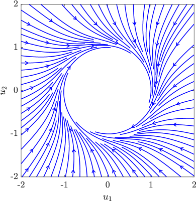
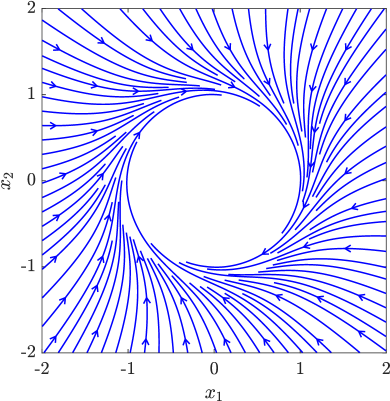
Figure 4: Example 4: Phase portraits for the true system (32) (left) and the learned system (33) (right).

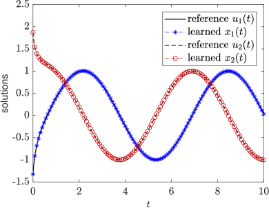
Figure 5: Example 4: Validation of the recovered system (33) with initial state $(-1.325,1.874)$. Left: solutions. Right: error $\|{\bf x}(t)-{\bf u}(t)\|_{2}$. The horizontal axis denotes the time.

We now consider data only with standard random noises and study the effect of noise level on the accuracy of recovered equations. Suppose we have $M=40$ sets of trajectory data with $J_{m}=10$, and all the data contain i.i.d. random noises following uniform distribution in $[-\eta,\eta]$. Here the parameter $\eta$ represents the noise level, and $\eta=0$ corresponds to noiseless data. The errors of the expansion coefficients in the learned systems are displayed in Fig. 6, for different noise levels at $\eta=0,0.005,0.01,0.05,0.1,0.2$. The vector 2-norms of the coefficient errors are shown in Fig. 7. It is clearly seen that the errors become larger at larger noise level in the data, which is not surprising.

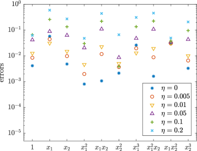
(a) Errors in coefficients $\mathbf{c}_{1}$

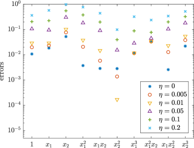
(b) Errors in coefficients $\mathbf{c}_{2}$

Figure 6: Example 4: Errors in each terms of the recovered equation at different noise levels.

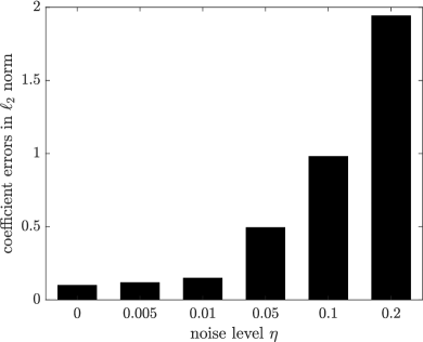
Figure 7: Example 4: The $\ell_{2}$ norm of the errors in the recovered coefficients of the equations.

Example 5

We now consider a damped pendulum problem. Let $l$ be the length of the pendulum, $\alpha$ be the damping constant, and $g$ be the gravitational constant. Then, for the unit mass, the governing equation is well known as

$$\frac{d^{2}\theta}{dt^{2}}+\frac{\alpha}{l}\frac{d\theta}{dt}+\frac{g}{l}\sin\theta=0,$$

where $\theta$ is the angle from its equilibrium vertical position. By defining $u_{1}=\theta$ and $u_{2}=\dot{\theta}$, we rewrite the equation as

$$\begin{cases}\dot{u}_{1}=u_{2},\\ \dot{u}_{2}=-\frac{g}{l}\sin u_{1}-\frac{\alpha}{l}u_{2}.\end{cases}$$ (34)

We set $l=1.1$ and $\alpha=0.22$, and use a large number of short trajectory data ($M=200,J_{m}=2$) to recover the equation. The initial state of each trajectory is randomly and uniformly chosen from the region $D=[-\pi,\pi]\times[-2\pi,2\pi]$. The least squares $\ell_{2}$-regression is used, with polynomial approximation at different degrees $n$. Figure 8 shows the phase portraits for the system (34) and the learned systems. As $n$ increases, the recovered dynamics becomes more accurate and can capture the true structures of the solution. More detailed examination of the learned system is shown in Figure 9, with polynomial degree $n=6$. We observe good agreements between the solution of the learned system ${\bf x}(t)$ and true solution ${\bf u}(t)$, at an arbitrarily chosen initial state $(-1.193,-3.876)$. The error evolution over time remains bounded at $10^{-2}$ level.

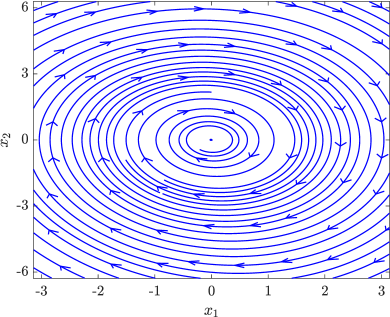
(a) $n=2$

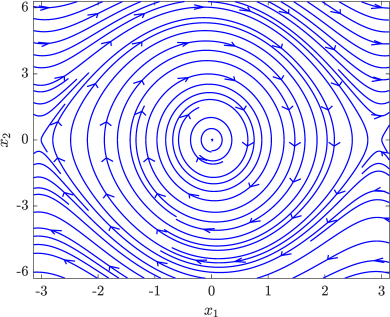
(b) $n=4$

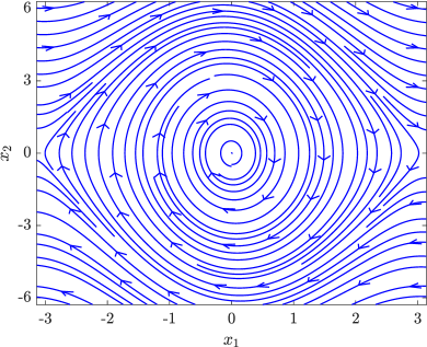
(c) $n=6$

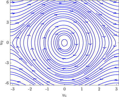
(d) Exact

Figure 8: Example 5: Phase portraits for the system (34) and its approximate systems learned from measurement data with different $n$.

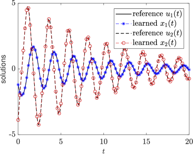
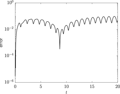
Figure 9: Example 5: Validation of the recovered system ($n=6$) with initial state $(-1.193,-3.876)$. Left: solutions. Right: error $\|{\bf x}(t)-{\bf u}(t)\|_{2}$. The horizontal axis denotes the time.

4.3 Nonlinear DAEs

We now study semi-explicit DAEs (5b) from measurement data. The learned approximating DAEs are denoted by

$$\dfrac{d{\bf x}(t)}{dt}={\tilde{\bf f}}({\bf x}(t)),$$ (35a)

$${\bf y}(t)=\tilde{\bf g}({\bf x}(t)),$$ (35b)

where ${\bf x}(t)$ and ${\bf y}(t)$ are approximations to ${\bf u}(t)$ and ${\bf v}(t)$, respectively. In the tests, the measurement data are first generated by numerically solving the true DAEs using the forth-order explicit Runge-Kutta method with a small time step-size. Possible noises or corruption errors are then added to the trajectories to generate our synthetic data.

Example 6

The first DAEs model we consider is a model for nonlinear electric network [28], defined as

$$\begin{cases}\dot{u}_{1}=v_{2}/C,\\ \dot{u}_{2}=u_{1}/L,\\ 0=v_{1}-(G_{0}-G_{\infty})U_{0}{\rm tanh}(u_{1}/U_{0})-G_{\infty}u_{1},\\ 0=v_{2}+u_{2}+v_{1},\end{cases}$$ (36)

where $u_{1}$ denotes the node voltage, and $u_{2}$, $v_{1}$ and $v_{2}$ are branch currents. Following [28], the physical parameters are specified as $C=10^{-9}$, $L=10^{-6}$, $U_{0}=1$, $G_{0}=-0.1$ and $G_{\infty}=0.25$. In our test, $D=[-2,2]\times[-0.2,0.2]$, $M=200$ sequences of trajectory data with $\Delta t=10^{-9}$ and $J_{m}=19$ are generated by numerically solving (36) and then adding random noises. The added noises in $u_{1}$ and $u_{2}$ follow uniform distribution on $[-0.0001,0.0001]$, while the noises in $v_{1}$ and $v_{2}$ follow normal distribution $N(0,0.001^{2})$ and $N(0,0.005^{2})$ respectively. We then use the $\ell_{2}$-regression with $n=8$ to learn the governing equations from these data. The phase portraits for the system $\dot{\bf u}={\bf f}({\bf u})$ and the learned system $\dot{\bf x}=\tilde{\bf f}({\bf x})$ are compared in Figure 10. It is observed that the proposed method accurately reproduces the dynamics and detects the correct features. Comparison the solutions between the recovered DAEs and the true system is shown Figure 11, using an arbitrary choice of the initial state $(0,0.1)$. The evolution of the numerical errors in the solution of the learned system are shown in Figure 12.

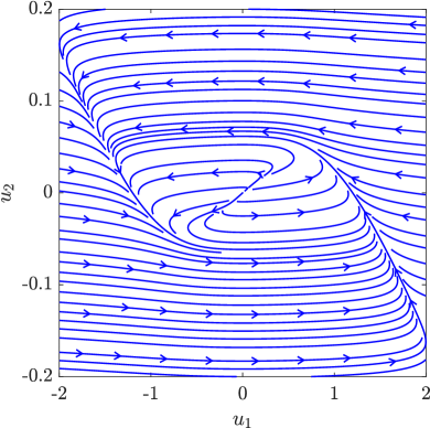
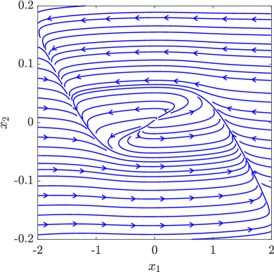
Figure 10: Example 6: Phase portraits for the system $\dot{\bf u}={\bf f}({\bf u})$ (left) and the learned system $\dot{\bf x}=\tilde{\bf f}({\bf x})$ (right).

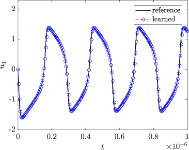
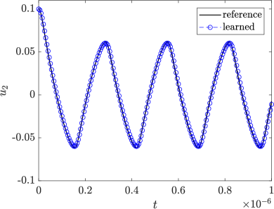
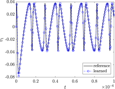
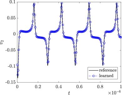
Figure 11: Example 6: Validation of the recovered system with initial state $(0,0.1)$. The solid lines denote the solution of the exact system, and the symbols “$\circ$” represent the solution of the learned system. The horizontal axis denotes the time.

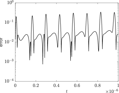
Figure 12: Example 6: Same as Figure 11 except for the errors $\|{\bf x}(t)-{\bf u}(t)\|_{2}$ (left) and $\|{\bf y}(t)-{\bf v}(t)\|_{2}$ (right).

Example 7

We now consider a model for a genetic toggle switch in Escherichia coli, which was proposed in [17] and numerically studied in [47]. It is composed of two repressors and two constitutive promoters, where each promoter is inhibited by the repressor that is transcribed by the opposing promoter. Details of experimental measurement can be found in [10], where the following model was also constructed,

$$\begin{cases}\dot{u}_{1}=\displaystyle{\frac{\alpha_{1}}{1+u_{2}^{\beta}}}-u_{1},\\ \dot{u}_{2}=\displaystyle{\frac{\alpha_{2}}{1+v_{1}^{\gamma}}}-u_{2},\\ 0=v_{1}+\varepsilon\sin v_{1}-\frac{u_{1}}{(1+{\rm[IPTG]}/K)^{\eta}}.\end{cases}$$ (37)

In the last equation, we add a small perturbation term $\varepsilon\sin v_{1}$ to increase the nonlinearity. Here, $u_{1}$ and $u_{2}$ are the concentration of the two repressors, respectively; $\alpha_{1}$ and $\alpha_{2}$ are the effective rates of synthesis of the repressors; $\gamma$ and $\beta$ represent cooperativity of repression of the two promoters, respectively; and $\rm[IPTG]$ is the concentration of IPTG, the chemical compound that induces the switch. The values of these parameters are taken as $\alpha_{1}=156.25$, $\alpha_{2}=15.6$, $\beta=2.5$, $\gamma=1$, $\eta=2.0015$. In the test, $D=[0,20]^{2}$ and we generate the measurement data by numerically solving (37) with $\rm[IPTG]=10^{-5}$ and $\varepsilon=0.01$. Suppose we have $M=500$ bursts of trajectory data with $J_{m}=2$, and five ($5$) arbitrarily chosen bursts of data contain corruption errors following normal distribution $N(1,1)$. We employ the $\ell_{1}$-regression approach with $n=16$ order of nominalized Legendre polynomial basis. The phase portraits for the system $\dot{\bf u}={\bf f}({\bf u})$ and the learned system $\dot{\bf x}=\tilde{\bf f}({\bf x})$ are plotted in Figure 13. As we can see, the learned structures agree well with the ideal structures everywhere in $D$. This demonstrates the ability of our method in finding the underlying governing equations. The accuracy of the learned model is further examined in Figures 14 and 15.

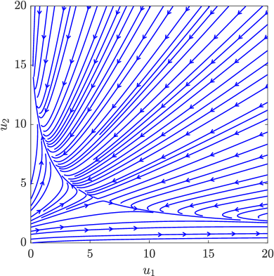
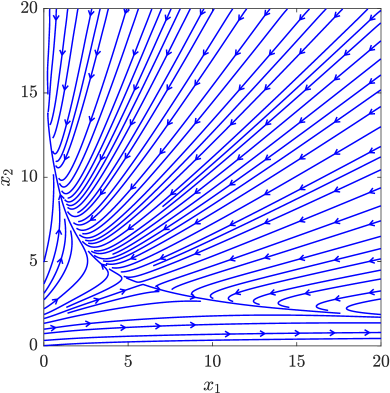
Figure 13: Example 7: Phase portraits for the system $\dot{\bf u}={\bf f}({\bf u})$ (left) and the learned system $\dot{\bf x}=\tilde{\bf f}({\bf x})$ (right).

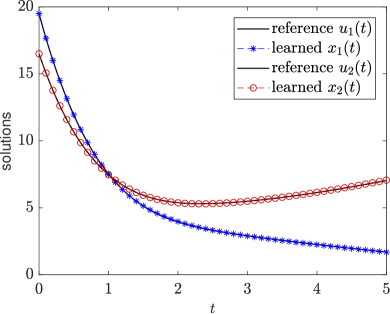
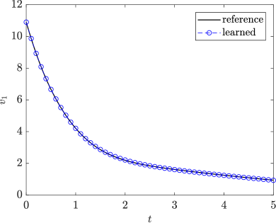
Figure 14: Example 7: Validation of the recovered system with initial state $(19.5,16.5)$. The horizontal axis denotes the time.

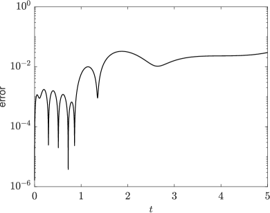
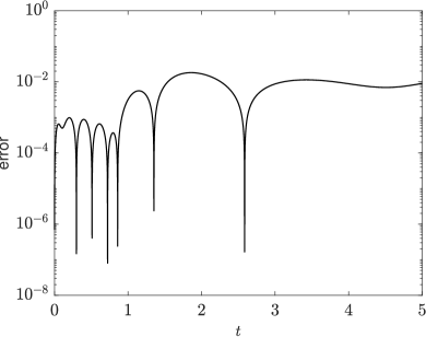
Figure 15: Example 7: Same as Figure 14 except for the errors $\|{\bf x}(t)-{\bf u}(t)\|_{2}$ (left) and $\|{\bf y}(t)-{\bf v}(t)\|_{2}$ (right).

Example 8

Our last example is a kinetic model of an isothermal batch reactor system, which was proposed in [2] and studied in [1, 20], among other literature. It was mentioned in [1] that the example in its original form was given by the Dow Chemical Company as a challenge test for parameter estimation methods. More details about this model can be found in [1]. The model consists of six differential mass balance equations, an electroneutrality condition and three equilibrium conditions,

$$\begin{cases}\dot{u}_{1}=-k_{2}u_{2}v_{2},\\ \dot{u}_{2}=-k_{1}u_{2}u_{6}+k_{-1}u_{4}-k_{2}u_{2}v_{2},\\ \dot{u}_{3}=k_{2}u_{2}v_{2}+k_{3}u_{4}u_{6}-k_{-3}v_{3},\\ \dot{u}_{4}=-k_{3}u_{4}u_{6}+k_{-3}v_{3},\\ \dot{u}_{5}=_{1}u_{2}u_{6}-k_{-1}v_{4},\\ \dot{u}_{6}=-k_{1}u_{2}u_{6}+k_{-1}v_{4}-k_{3}v_{4}v_{6}+k_{-3}v_{3},\\ {\rm[Q^{+}]}-u_{6}+v_{1}-v_{2}-v_{3}-v_{4}=0,\\ v_{2}-K_{2}u_{1}/(K_{2}+v_{1})=0,\\ v_{3}-K_{3}u_{3}/(K_{3}+v_{1})=0,\\ v_{4}-K_{1}u_{5}/(K_{1}+v_{1})=0.\end{cases}$$ (38)

In our test, the values of the parameters are specified as $k_{1}=25.1911$, $k_{2}=43.1042$, $k_{-1}=1.1904\times 10^{5}$, $k_{-3}=\frac{1}{2}k_{-1}$, $K_{1}=2.575\times 10^{-2}$, $K_{2}=4.876$, and $K_{3}=1.7884\times 10^{-2}$, and ${\rm[Q^{+}]}=0.0131$. Assume that one can collect many sets of the time-series measurement data of ${\bf u}$ and ${\bf v}$ starting from any initial states ${\bf u}_{0}^{(m)}\in D=[0.6,1.6]\times[6.5,8.5]\times[0,0.7]\times[0,0.3]\times[0,0.3]\times[0,0.02]$. We collect $500,000$ bursts of trajectory data with $\Delta t=10^{-4}$, $J_{m}=2$ and ${\bf u}_{0}^{(m)}$ sampled from the tensorized Chebyshev distribution on $D$. The data set is big as to enable possible accurate discovery of the complicated reaction process. Handling such a (relatively) large-scale problem with the standard regression algorithms can be challenging, primarily due to the large size of matrices. Without using more sophisticated regression methods to deal with large matrices (which is a topic outside our scope), we employ the sequential approximation (SA) algorithm to demonstrate its capability of handling large data sets. We employ the nominalized Legendre polynomial basis of up to order $n=12$. This induces $N=18,564$ basis functions. The convergence result is examined by the errors in the function approximation $\tilde{\bf f}^{(k)},\tilde{\bf g}^{(k)}$ in the $k$-th step iteration compared with the exact functions ${\bf f},{\bf g}$. To evaluate the errors we independently draw a set of 20,000 samples uniformly and compute the difference between $\tilde{\bf f}^{(k)},\tilde{\bf g}^{(k)}$ and ${\bf f},{\bf g}$ at these sampling points. The vector 2-norm is then used to report the difference. The relative errors in each iteration of SA are displayed in Figure 16 with respect to the number of iterations $k$. The SA method uses one piece of data at a time, and exhibits good effectiveness in this case. As the iteration continues, more data are used and more accurate approximations are obtained, yielding more accurate models. The exponential type convergence of the errors is observed. This is consistent with the theoretical analysis in [39, 46, 37]. We also validate the finial system with the initial state ${\bf u}_{0}=(1.5776,8.32,0,0,0,0.0142)^{\top}$, and observe good agreements between the solutions of the recovered system and the exact system in Figure 17.

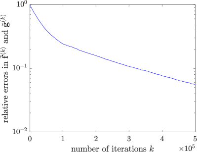
Figure 16: Example 8: Convergence history of the sequential approximation.

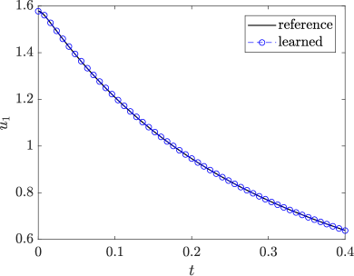
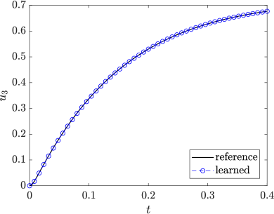
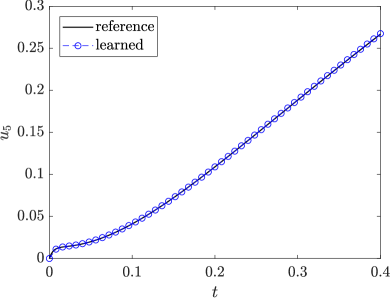
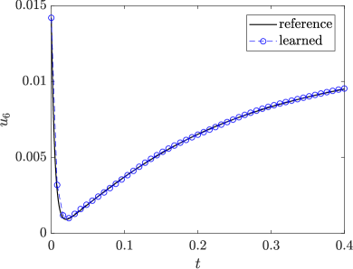
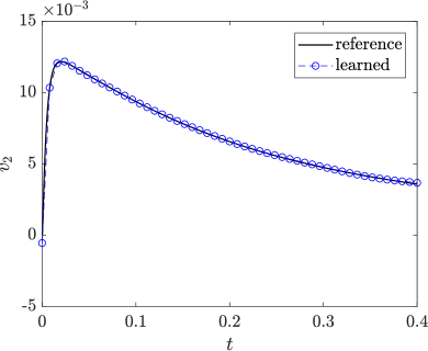
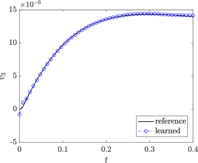
Figure 17: Example 8: Validation of the learned system. The solid lines denote the solution of the exact system, and the symbols “$\circ$” represent the solution of the learned system. The horizontal axis denotes the time.

5 Conclusion

In this paper we studied several effective numerical algorithms for data-driven discovery of nonlinear differential/algebraic equations. We proposed to use the standard basis functions such as polynomials to construct accurate approximation of the true governing equations, rather than the exact recovery. We also discussed the importance of using a (large) number of short bursts of trajectory data, rather than data from a single (long) trajectory. In conjunction with some standard approximation algorithms, e.g., least squares method, the overall method can produce highly accurate approximation of the true governing equations. Using an extensive set of test examples, ranging from textbook examples to more complicated practical examples, we demonstrated that the proposed method can be highly effective in many situations.

Appendix A Proof of Theorem 1

We first introduce the following lemma.

Lemma 1

If ${\bf f}\in L^{\infty}(D)$, we have

$$\|\tilde{\bf f}-{\bf f}\|_{2,L^{\infty}}\leq\|{\bf f}-{\mathcal{P}}_{V}{\bf f}\|_{2,L^{\infty}}+\|\tilde{\bf f}-{\mathcal{P}}_{V}{\bf f}\|_{2,L^{2}_{\omega}}\|\sqrt{K}\|_{L^{\infty}}.$$ (39)

Proof

The triangular inequality gives

$$\|\tilde{\bf f}-{\bf f}\|_{2,L^{\infty}}\leq\|{\bf f}-{\mathcal{P}}_{V}{\bf f}\|_{2,L^{\infty}}+\|\tilde{\bf f}-{\mathcal{P}}_{V}{\bf f}\|_{2,L^{\infty}}.$$ (40)

Let ${\bf\Psi}=(\psi_{1},\cdots,\psi_{N})^{\top}$ be any orthogonal basis of $V$, and

$${\mathcal{P}}_{V}f_{\ell}=:\langle\hat{\bf c}_{\ell},{\bf\Psi}({\bf x})\rangle,\qquad\tilde{f}_{\ell}=:\langle\tilde{\bf c}_{\ell},{\bf\Psi}({\bf x})\rangle.$$

Then $K(\mathbf{x})=\|{\bf\Psi}(\mathbf{x})\|_{2}^{2}$. Note for any ${\bf x}\in D$ that

$$\|\tilde{\bf f}({\bf x})-{\mathcal{P}}_{V}{\bf f}({\bf x})\|_{2}^{2} = \sum_{\ell=1}^{d}\big{|}\tilde{f}_{\ell}({\bf x})-{\mathcal{P}}_{V}f_{\ell}({\bf x})\big{|}^{2}=\sum_{\ell=1}^{d}\big{|}\langle\tilde{\bf c}_{\ell}-\hat{\bf{c}}_{\ell},{\bf\Psi}({\bf x})\rangle\big{|}^{2}$$

$$\leq \sum_{\ell=1}^{d}\|\tilde{\bf c}_{\ell}-\hat{\bf{c}}_{\ell}\|_{2}^{2}\|{\bf\Psi}({\bf x})\|_{2}^{2}=\sum_{\ell=1}^{d}\|\tilde{f}_{\ell}-{\mathcal{P}}_{V}f_{\ell}\|_{L^{2}_{\omega}}^{2}K(\mathbf{x})$$

$$= \|\tilde{\bf f}-{\mathcal{P}}_{V}{\bf f}\|_{2,L^{2}_{\omega}}^{2}K(\mathbf{x}),$$

where the Cauchy-Schwarz inequality and the orthogonality of basis $\{\psi_{j}(\mathbf{x})\}$ have been used. Taking $L^{\infty}$-norm in the above inequality and using (40) give (39). $\square$

Based on the above lemma, the proof of Theorem 1 is given as follows.

Proof

Integrating the systems (1) and (11) respectively gives

$${\bf u}(t)={\bf u}(t_{0})+\int_{t_{0}}^{t}{\bf f}({\bf u}(s))ds,$$ (41)

$${\bf x}(t)={\bf x}(t_{0})+\int_{t_{0}}^{t}\tilde{\bf f}({\bf x}(s))ds.$$ (42)

Subtracting (41) from (42) with ${\bf u}(t_{0})={\bf x}(t_{0})$, we obtain

$$\big{\|}{\bf x}(t)-{\bf u}(t)\big{\|}_{2} = \bigg{\|}\int_{t_{0}}^{t}\tilde{\bf f}({\bf x}(s))-{\bf f}({\bf u}(s))ds\bigg{\|}_{2}$$

$$= (t-t_{0})\eta\bigg{(}\frac{1}{t-t_{0}}\int_{t_{0}}^{t}\tilde{\bf f}({\bf x}(s))-{\bf f}({\bf u}(s))ds\bigg{)},$$

where $\eta({\bf x})=\|{\bf x}\|_{2}$ is a convex function satisfying the Jensen’s inequality

$$\eta\bigg{(}\frac{1}{t-t_{0}}\int_{t_{0}}^{t}\tilde{\bf f}({\bf x}(s))-{\bf f}({\bf u}(s))ds\bigg{)}\leq\frac{1}{t-t_{0}}\int_{t_{0}}^{t}\eta\big{(}\tilde{\bf f}({\bf x}(s))-{\bf f}({\bf u}(s))\big{)}ds.$$

This together with the triangular inequality yield

$$\big{\|}{\bf x}(t)-{\bf u}(t)\big{\|}_{2} \leq \int_{t_{0}}^{t}\big{\|}\tilde{\bf f}({\bf x}(s))-{\bf f}({\bf u}(s))\big{\|}_{2}ds$$

$$\leq \int_{t_{0}}^{t}\big{\|}\tilde{\bf f}({\bf x}(s))-{\bf f}({\bf x}(s))\big{\|}_{2}+\big{\|}{\bf f}({\bf x}(s))-{\bf f}({\bf u}(s))\big{\|}_{2}ds$$

$$\leq \int_{t_{0}}^{t}\|\tilde{\bf f}-{\bf f}\|_{2,L^{\infty}}+L_{f}\big{\|}{\bf x}(s)-{\bf u}(s)\big{\|}_{2}ds,$$

which implies (25). Applying Grönwall’s inequality to (25) gives

$$\big{\|}{\bf x}(t)-{\bf u}(t)\big{\|}_{2} \leq \bigg{(}t-t_{0}+L_{f}\int_{t_{0}}^{t}(s-t_{0})\exp\big{(}L_{f}(t-s)\big{)}ds\bigg{)}\|\tilde{\bf f}-{\bf f}\|_{2,L^{\infty}}$$

$$= L_{f}^{-1}\big{(}e^{L_{f}(t-t_{0})}-1\big{)}\|\tilde{\bf f}-{\bf f}\|_{2,L^{\infty}},$$

Then utilizing (39), we get (26) and complete the proof. $\square$

References

References

- [1] V. M. Becerra, P. D. Roberts, and G. W. Griffiths. Applying the extended Kalman filter to systems described by nonlinear differential-algebraic equations. Control Eng. Pract., 9(3):267–281, 2001.
- [2] L. T. Biegler, J. J. Damiano, and G. E. Blau. Nonlinear parameter estimation: a case study comparison. AIChE Journal, 32(1):29–45, 1986.
- [3] J. Bongard and H. Lipson. Automated reverse engineering of nonlinear dynamical systems. Proc. Natl. Acad. Sci. U.S.A., 104(24):9943–9948, 2007.
- [4] W. E. Boyce and R. C. DiPrima. Elementary differential equations and boundary value problems, 2009.
- [5] S. Brunton, J. N. Kutz, and J. Proctor. Data-driven discovery of governing physical laws. SIAM News, 50:1, 2017.
- [6] S. L. Brunton, B. W. Brunton, J. L. Proctor, Eurika Kaiser, and J. N. Kutz. Chaos as an intermittently forced linear system. Nature Communications, 8, 2017.
- [7] S. L. Brunton, J. L. Proctor, and J. N. Kutz. Discovering governing equations from data by sparse identification of nonlinear dynamical systems. Proc. Natl. Acad. Sci. U.S.A., 113(15):3932–3937, 2016.
- [8] E. Candes and J. Romberg. -MAGIC: Recovery of Sparse Signals via Convex Programming. www.acm.caltech.edu/l1magic/downloads/l1magic.pdf, 2005.
- [9] E. J. Candes and T. Tao. Decoding by linear programming. IEEE Trans. Inform. Theory, 51(12):4203–4215, 2005.
- [10] R. Chartrand. Numerical differentiation of noisy, nonsmooth data. ISRN Applied Mathematics, 2011, 2011.
- [11] E.W. Cheney. Introduction to Approximation theory. McGraw-Hill, New York, 1966.
- [12] J. P. Crutchfield and B. S. McNamara. Equations of motion from a data series. Complex Systems, 1(417-452):121, 1987.
- [13] Jane Cullum. Numerical differentiation and regularization. SIAM J. Numer. Anal., 8(2):254–265, 1971.
- [14] B. C. Daniels and I. Nemenman. Automated adaptive inference of phenomenological dynamical models. Nature Communications, 6, 2015.
- [15] B. C. Daniels and I. Nemenman. Efficient inference of parsimonious phenomenological models of cellular dynamics using S-systems and alternating regression. PloS One, 10(3):e0119821, 2015.
- [16] P.J. Davis. Interpolation and approximation. Dover, 1975.
- [17] T. S. Gardner, C. R. Cantor, and J. J. Collins. Construction of a genetic toggle switch in escherichia coli. Nature, 403(6767):339, 2000.
- [18] D. Giannakis and A. J. Majda. Nonlinear Laplacian spectral analysis for time series with intermittency and low-frequency variability. Proc. Natl. Acad. Sci. U.S.A., 109(7):2222–2227, 2012.
- [19] R. Gonzalez-Garcia, R. Rico-Martinez, and I. G. Kevrekidis. Identification of distributed parameter systems: A neural net based approach. Comput. Chem. Eng., 22:S965–S968, 1998.
- [20] S. C. Kadu, M. Bhushan, R. Gudi, and K. Roy. Modified unscented recursive nonlinear dynamic data reconciliation for constrained state estimation. J. Process Control, 20(4):525–537, 2010.
- [21] I. G. Kevrekidis, C. W. Gear, J. M. Hyman, P. G. Kevrekidid, O. Runborg, C. Theodoropoulos, et al. Equation-free, coarse-grained multiscale computation: Enabling mocroscopic simulators to perform system-level analysis. Commun. Math. Sci., 1(4):715–762, 2003.
- [22] I. Knowles and R. J. Renka. Methods for numerical differentiation of noisy data. Electronic Journal of Differential Equations, 21(2012):235–246, 2014.
- [23] I. Knowles and R. Wallace. A variational method for numerical differentiation. Numer. Math., 70(1):91–110, 1995.
- [24] A. J. Majda, C. Franzke, and D. Crommelin. Normal forms for reduced stochastic climate models. Proc. Natl. Acad. Sci. U.S.A., 106(10):3649–3653, 2009.
- [25] N. M. Mangan, S. L. Brunton, J. L. Proctor, and J. N. Kutz. Inferring biological networks by sparse identification of nonlinear dynamics. IEEE Transactions on Molecular, Biological and Multi-Scale Communications, 2(1):52–63, 2016.
- [26] N. M. Mangan, J. N. Kutz, S. L. Brunton, and J. L. Proctor. Model selection for dynamical systems via sparse regression and information criteria. Proceedings of the Royal Society of London A: Mathematical, Physical and Engineering Sciences, 473(2204), 2017.
- [27] M.J.D. Powell. Approximation theory and methods. Cambridge University Press, 1981.
- [28] R. Pulch. Polynomial chaos for semiexplicit differential algebraic equations of index 1. Int. J. Uncertain. Quantif., 3(1), 2013.
- [29] T.J. Rivlin. An introduction to the approximation of functions. Dover publication Inc, 1969.
- [30] A. J. Roberts. Model Emergent Dynamics in Complex Systems. SIAM, 2014.
- [31] S. H. Rudy, S. L. Brunton, J. L. Proctor, and J. N. Kutz. Data-driven discovery of partial differential equations. Science Advances, 3(4):e1602614, 2017.
- [32] H. Schaeffer and S. G. McCalla. Sparse model selection via integral terms. Phys. Rev. E, 96(2):023302, 2017.
- [33] H. Schaeffer, G. Tran, and R. Ward. Extracting sparse high-dimensional dynamics from limited data. arXiv preprint arXiv:1707.08528, 2017.
- [34] Hayden Schaeffer. Learning partial differential equations via data discovery and sparse optimization. Proceedings of the Royal Society of London A: Mathematical, Physical and Engineering Sciences, 473(2197), 2017.
- [35] M. Schmidt and H. Lipson. Distilling free-form natural laws from experimental data. Science, 324(5923):81–85, 2009.
- [36] M. D. Schmidt, R. R. Vallabhajosyula, J. W. Jenkins, J. E. Hood, A. S. Soni, J. P. Wikswo, and H. Lipson. Automated refinement and inference of analytical models for metabolic networks. Physical Biology, 8(5):055011, 2011.
- [37] Y. Shin, K. Wu, and D. Xiu. Sequential function approximation with noisy data. J. Comput. Phys., 371:363–381, 2018.
- [38] Y. Shin and D. Xiu. Correcting data corruption errors for multivariate function approximation. SIAM J. Sci. Comput., 38(4):A2492–A2511, 2016.
- [39] Y. Shin and D. Xiu. A randomized algorithm for multivariate function approximation. SIAM J. Sci. Comput., 39(3):A983–A1002, 2017.
- [40] G. Sugihara, R. May, H. Ye, C. Hsieh, E. Deyle, M. Fogarty, and S. Munch. Detecting causality in complex ecosystems. Science, 338(6106):496–500, 2012.
- [41] R. Tibshirani. Regression shrinkage and selection via the lasso. Journal of the Royal Statistical Society. Series B (Methodological), pages 267–288, 1996.
- [42] G. Tran and R. Ward. Exact recovery of chaotic systems from highly corrupted data. Multiscale Model. Simul., 15(3):1108–1129, 2017.
- [43] H. U. Voss, P. Kolodner, M. Abel, and J. Kurths. Amplitude equations from spatiotemporal binary-fluid convection data. Phys. Rev. Lett., 83(17):3422, 1999.
- [44] J. Wagner, P. Mazurek, and R. Z. Morawski. Regularised differentiation of measurement data. In XXI IMEKO World Congress “Measurement in Research and Industry”. Prague, Czech Republic, 2015.
- [45] K. Wu, Y. Shin, and D. Xiu. A randomized tensor quadrature method for high dimensional polynomial approximation. SIAM J. Sci. Comput., 39:A1811–A1833, 2017.
- [46] K. Wu and D. Xiu. Sequential function approximation on arbitrarily distributed point sets. J. Comput. Phys., 354:370–386, 2018.
- [47] D. Xiu. Efficient collocational approach for parametric uncertainty analysis. Commun. Comput. Phys., 2(2):293–309, 2007.
- [48] H. Ye, R. J. Beamish, S. M. Glaser, S. C. H. Grant, C. Hsieh, L. J. Richards, J. T. Schnute, and G. Sugihara. Equation-free mechanistic ecosystem forecasting using empirical dynamic modeling. Proc. Natl. Acad. Sci. U.S.A., 112(13):E1569–E1576, 2015.
- [49] T. Zhou, A. Narayan, and D. Xiu. Weighted discrete least-squares polynomial approximation using randomized quadratures. J. Comput. Phys., 298:787–800, 2015.