Cosmology from cosmic shear power spectra with Subaru Hyper Suprime-Cam first-year data

Abstract

We measure cosmic weak lensing shear power spectra with the Subaru Hyper Suprime-Cam (HSC) survey first-year shear catalog covering 137 deg² of the sky. Thanks to the high effective galaxy number density of $\sim 17$ arcmin^-2 even after conservative cuts such as magnitude cut of $i<24.5$ and photometric redshift cut of $0.3\leq z\leq 1.5$, we obtain a high significance measurement of the cosmic shear power spectra in 4 tomographic redshift bins, achieving a total signal-to-noise ratio of 16 in the multipole range $300\leq\ell\leq 1900$. We carefully account for various uncertainties in our analysis including the intrinsic alignment of galaxies, scatters and biases in photometric redshifts, residual uncertainties in the shear measurement, and modeling of the matter power spectrum. The accuracy of our power spectrum measurement method as well as our analytic model of the covariance matrix are tested against realistic mock shear catalogs. For a flat $\Lambda$ cold dark matter ($\Lambda$CDM) model, we find $S_{8}\equiv\sigma_{8}(\Omega_{\rm m}/0.3)^{\alpha}=0.800^{+0.029}_{-0.028}$ for $\alpha=0.45$ ($S_{8}=0.780^{+0.030}_{-0.033}$ for $\alpha=0.5$) from our HSC tomographic cosmic shear analysis alone. In comparison with Planck cosmic microwave background constraints, our results prefer slightly lower values of $S_{8}$, although metrics such as the Bayesian evidence ratio test do not show significant evidence for discordance between these results. We study the effect of possible additional systematic errors that are unaccounted in our fiducial cosmic shear analysis, and find that they can shift the best-fit values of $S_{8}$ by up to $\sim 0.6\sigma$ in both directions. The full HSC survey data will contain several times more area, and will lead to significantly improved cosmological constraints.

1 Introduction

The $\Lambda$ Cold Dark Matter ($\Lambda$CDM) model has been established as the standard cosmological model to describe the expansion history and the growth of the large-scale structure of the Universe. Assuming the $\Lambda$CDM model, cosmological parameters have been measured within percent-level uncertainties by a combination of observations such as the cosmic microwave background (CMB) experiments (e.g., Hinshaw et al., 2013; Planck Collaboration et al., 2016, 2018), type-Ia supernovae (e.g., Suzuki et al., 2012; Betoule et al., 2014), and baryon acoustic oscillations (BAO; e.g., Anderson et al., 2014; Alam et al., 2017). Despite the success of the model, we are challenged by a fundamental lack of physical understanding of the main components of the Universe, dark matter and cosmological constant $\Lambda$ or more generally dark energy. In order to understand these dark components, it is of great importance to test the $\Lambda$CDM model at high precision using a variety of cosmological probes.

Weak gravitational lensing provides an important means of studying the mass distribution of the Universe including dark matter, because it is a purely gravitational effect. In particular, the coherent distorted pattern of distant galaxy images by gravitational lensing of large-scale structure, commonly referred to as the cosmic shear signal, is a powerful probe of the matter distribution in the Universe (Blandford et al., 1991; Miralda-Escude, 1991; Kaiser, 1992). Cosmic shear, the two-point correlation function or power spectrum of the weak lensing signal, depends on both the growth of the matter density field and the expansion history of the Universe, and serves as a unique cosmological probe. It allows us to test a range of cosmological models including dynamical dark energy and modified gravity (see Bartelmann & Schneider, 2001; Kilbinger, 2015, for reviews). Since the first detections of cosmic shear around 2000 (Bacon et al., 2000; Van Waerbeke et al., 2000; Wittman et al., 2000; Kaiser et al., 2000; Maoli et al., 2001; Rhodes et al., 2001; Van Waerbeke et al., 2001; Hoekstra et al., 2002; Bacon et al., 2003; Jarvis et al., 2003; Brown et al., 2003; Hamana et al., 2003), cosmic shear studies have progressed in their precision thanks to the progress of wide-field imaging surveys. For instance, the Canada-France-Hawaii Telescope Lensing Survey (CFHTLS) survey observed $\sim 10^{7}$ galaxies over 154 square degrees of the sky (CFHTLenS; Heymans et al., 2012) to conduct tomographic analyses (Hu, 1999) of cosmic shear (Heymans et al., 2013; Kilbinger et al., 2013; Kitching et al., 2014). The Deep Lens survey (DLS) conducted a deep cosmic shear analysis using galaxies with a limiting magnitude 27 mag in $R$-band over 20 square degrees of the sky (Jee et al., 2016). Galaxy imaging surveys for even wider areas, which are known as “Stage III” surveys, are on-going (Albrecht et al., 2006). These Stage III surveys, which include the Kilo-Degree survey (KiDS; Kuijken et al., 2015), the Dark Energy Survey (DES; Abbott et al., 2016; Becker et al., 2016), and the Hyper Suprime-Cam (HSC) survey (Aihara et al., 2018b, a), are expected to yield constraints on cosmological parameters from the cosmic shear analyses that are competitive with other dark energy probes. Cosmic shear is especially sensitive to the combination of the matter density parameter $\Omega_{\rm m}$ and the amplitude parameter of matter fluctuations $\sigma_{8}$, i.e., $S_{8}(\alpha)\equiv\sigma_{8}(\Omega_{\rm m}/0.3)^{\alpha}$ with $\alpha\sim 0.5$. In the next decade, we expect that “Stage IV” galaxy surveys such as the Large Synoptic Survey Telescope (LSST; LSST Science Collaboration et al., 2009), the Wide Field Infrared Survey Telescope (WFIRST; Spergel et al., 2015) and Euclid (Laureijs et al., 2011) will provide even more accurate measurements of cosmic shear from observations of $\sim 10^{9}$ galaxies over thousands of square degrees.

Accurate cosmic shear measurements are needed in order to test the concordance between the cosmological parameters obtained from the Planck CMB experiment, which is based on high redshift linear physics, and lensing surveys which are based on much lower redshifts and non-linear physics. In the flat $\Lambda$CDM model, the Planck temperature and polarization power spectra (without CMB lensing) constrain $S_{8}(\alpha=0.5)$ to be $0.848\pm 0.024$ (Planck Collaboration et al., 2016), whereas several lensing surveys infer values of $S_{8}$ lower by about 2-3$\sigma$, e.g., $0.757^{+0.033}_{-0.038}$ from the KiDS-450 correlation function analysis (Hildebrandt et al., 2017), $0.651\pm 0.058$ from the KiDS-450 power spectrum analysis (Köhlinger et al., 2017), $0.732^{+0.029}_{-0.031}$ from CFHTLenS (Joudaki et al., 2017a, for the fiducial case where systematics are not included), and $0.782^{+0.027}_{-0.027}$ from DES year one (Y1) data (Troxel et al., 2018a). While the original constraints on $S_{8}$ from DLS is consistent with Planck, $0.818^{+0.034}_{-0.026}$ (Jee et al., 2016), Chang et al. (2019) shows that the $S_{8}$ value decreases to $0.795\pm 0.032$ when the fitting formula of the nonlinear matter power spectrum is updated from Smith et al. (2003) to Takahashi et al. (2012). The tension may indicate physics beyond the $\Lambda$CDM model such as dynamical dark energy or modified gravity (e.g., Amendola et al., 2018), and therefore the possible systematic effects should be carefully examined (see also Troxel et al., 2018b; Chang et al., 2019).

The Hyper Suprime-Cam Subaru Strategic Program (HSC-SSP, hereafter the HSC survey) is a wide-field imaging survey using a 1.77 deg² field-of-view imaging camera on the 8.2-meter Subaru telescope (Miyazaki et al., 2012, 2015, 2018; Komiyama et al., 2018; Furusawa et al., 2018; Kawanomoto et al., 2018). The HSC survey is unique due to the combination of its depth ($5\sigma$ point-source depth of the Wide layer of $i\sim 26$) and excellent image quality (typical $i$-band seeing of $\sim 0\farcs 58$), which enable us to measure cosmic shear signals up to higher redshifts with lower shape noise than KiDS and DES. The data from the first 1.7 years (61.5 nights) was publicly released in Feb 2017 (Aihara et al., 2018a). Mandelbaum et al. (2018a) present the first-year shear catalog (Y1) for weak lensing science, and carry out intensive null tests of the catalog against various possible systematics such as errors in the point-spread function (PSF) modeling and biases in the shear estimation. These null tests demonstrated that the shear catalog meets the requirements for carrying out science from this data without being significantly affected by systematics. Here the requirements we set are that residual systematic errors identified from the data are sufficiently smaller than the overall statistical error in a measurement of the cosmic shear correlation function, where the overall statistical error indicates a total signal-to-noise ratio of the correlation function measurement estimated using the HSC mock shear catalogs. Oguri et al. (2018) have reconstructed two- and three-dimensional mass maps from the first-year shear catalog. They found significant correlations between the mass maps and projected galaxy maps, and no statistically significant correlations between the mass maps and the maps of potential sources of systematics, further demonstrating that the first-year shear catalog is ready for science analyses.

In this paper, we present results from a tomographic cosmic shear analysis using the HSC first-year shear catalog. We adopt a pseudo-spectrum (hereafter pseudo-$C_{\ell}$) approach to obtain unbiased cosmic shear power spectra from incomplete sky data (Hikage et al., 2011; Hikage & Oguri, 2016). We perform a nested sampling analysis of the HSC cosmic shear power spectra to constrain cosmological parameters, especially focusing on $S_{8}$, in the context of the flat $\Lambda$CDM model. In order to obtain robust cosmological constraints from cosmic shear measurements, we take into account various systematic errors, and perform a blind analysis to avoid confirmation biases affecting our results. One of the systematic errors we consider is the measurement error of galaxy images due to imperfect modeling of the PSF and the deconvolution error of the PSF model from galaxy images (Mandelbaum et al., 2018a). We account for additive and multiplicative biases in our shape measurement method quantified by Mandelbaum et al. (2018b) using image simulations of the HSC survey. Another source of systematic errors is related to the photometric redshift (photo-$z$) uncertainties. Since it is not feasible to measure the spectroscopic redshifts of all galaxies used for the weak lensing analysis, the redshift distribution of source galaxies is inferred from just their photometric information (Tanaka et al., 2018). Intrinsic shape correlations due to tidal interactions also result in systematics in cosmic shear measurements (Hirata & Seljak, 2004; Joachimi et al., 2015; Kirk et al., 2015). There are also uncertainties in modeling the matter power spectrum on small scales due to baryonic effects such as star formation, supernovae, and AGN feedback (White, 2004; Zhan & Knox, 2004; Huterer & Takada, 2005; Jing et al., 2006; Bernstein, 2009; Semboloni et al., 2011). In addition to testing for these systematics, we conduct various internal consistency tests among different photo-$z$ bins, fields, and ranges of angular scales, as well as null tests of B-modes, to check the robustness of our results. We present tests for our cosmic shear measurement as well as analysis methods using realistic mock catalogs. We discuss the consistency of our constraints with Planck CMB data and other lensing surveys such as DES and KiDS, and also explore effects of the dark energy equation of state and non-zero neutrino mass.

This paper is organized as follows. In Section 2, we briefly describe the HSC first-year shear catalog that is used in our cosmic shear analysis. In Section 3, we describe and validate the pseudo-$C_{\ell}$ method to estimate unbiased cosmic shear spectra from finite-sky non-uniform data. In Section 4, we also show our measurements of tomographic cosmic shear spectra using the HSC first-year shear catalog. Section 5 summarizes model ingredients for our cosmological analysis, including predictions of cosmic shear signals and covariance and our methods to take account of various systematics in cosmic shear analysis. Our cosmological constraints and their robustness to different systematics are presented in Section 6. Finally we give our conclusions in Section 7.

Since the cosmological likelihoods for the final Planck data release (Planck Collaboration et al., 2018) are not yet available at the time of writing this paper, throughout this paper we use Planck 2015 CMB results (Planck Collaboration et al., 2016) for the comparison and the joint analysis with our HSC first-year cosmic shear measurement. We use the joint TT, EE, BB, and TE likelihoods for $\ell$ between 2 and 29 and the TT likelihood for $\ell$ between 30 and 2508, commonly referred to as Planck TT + lowP (Planck Collaboration et al., 2016). We do not use CMB lensing results, which contain information on the growth of structure and the expansion history of the Universe at late stages, except when we combine our joint analysis result with distance measurements using baryonic acoustic oscillations and Type Ia supernovae (Section 6.4).

Throughout this paper we quote 68% credible intervals for parameter uncertainties unless otherwise stated.

2 HSC first-year shear catalog

Hyper Suprime-Cam (HSC) is a wide-field imaging camera with 1.77 deg² field-of-view mounted on the prime focus of the 8.2-meter Subaru telescope (Miyazaki et al., 2012, 2015, 2018). The HSC survey is using 300 nights of Subaru time over 6 years to conduct a multi-band wide-field imaging survey with HSC. The HSC survey consists of three layers; Wide, Deep and UltraDeep. The Wide layer, which is specifically designed for weak lensing cosmology, aims at covering 1400 square degrees of the sky with five broadbands, $grizy$, with a $5\sigma$ point-source depth of $r\approx 26$ (Aihara et al., 2018b). Since $i$-band images are used for galaxy shape measurements for weak lensing analysis, $i$-band images are preferentially taken when the seeing is better. As a result, we achieve a median PSF FWHM of $\sim 0\farcs 58$ for the $i$-band images used to construct the HSC first-year shear catalog. The details of the software pipeline used to reduce the data are given in Bosch et al. (2018), and particulars about the accuracy of the photometry and the performance of the deblender are characterized using a synthetic imaging pipeline in Huang et al. (2018) and Murata et al. (in prep.), respectively. The HSC Subaru Strategic Program (SSP) Data Release 1 (DR1), based on data taken using 61.5 nights between March 2014 and November 2015, has been made public (Aihara et al., 2018a).

The HSC first-year shear catalog (Mandelbaum et al., 2018a) is based on about 90 nights of HSC Wide data taken from March 2014 to April 2016, which is larger than the public HSC DR1 data. We apply a number of cuts to construct a shape catalog for weak lensing analysis which satisfies the requirements for carrying out first year key science (see Mandelbaum et al., 2018a, for more details). For instance, we restrict our analysis to the regions of sky with approximately full depth in all 5 filters to ensure the homogeneity of the sample. We also adopt a cmodel magnitude cut of $i<24.5$ (see Bosch et al. 2018 for definition of cmodel magnitude in the context of HSC), which is conservative given that the magnitude limit of the HSC is $i\sim 26.4$ ($5\sigma$ for point sources; Aihara et al., 2018a). We remove galaxies with PSF modeling failures and those located in disconnected regions. Regions of sky around bright stars ($\sim 16\%$ of the total area) are masked (Mandelbaum et al., 2018a). As a result, the final weak lensing shear catalog covers 136.9 deg² that consists of 6 disjoint patches: XMM, GAMA09H, GAMA15H, HECTOMAP, VVDS, and WIDE12H. Mandelbaum et al. (2018a) and Oguri et al. (2018) performed extensive null tests of the shear catalog to show that the shear catalog satisfies the requirements of HSC first-year science for both cosmic shear and galaxy-galaxy lensing.

The shapes of galaxies are estimated on the $i$-band coadded images using the re-Gaussianization PSF correction method (Hirata & Seljak, 2003). An advantage of this method is that it has been applied extensively to Sloan Digital Sky Survey data, and thus the systematics of the method are well understood (Mandelbaum et al., 2005, 2013). In this method, the shape of a galaxy image is defined as

$$\bm{e}=(e_{1},e_{2})=\frac{1-(b/a)^{2}}{1+(b/a)^{2}}(\cos 2\phi,\sin 2\phi),$$ (1)

where $b/a$ is the observed minor-to-major axis ratio and $\phi$ is the position angle of the major axis with respect to the equatorial coordinate system. The shear of each galaxy, $\bm{\gamma}^{\rm(obs)}$, is estimated from the measured ellipticity $\bm{e}$ as follows:

$$\bm{\gamma}^{\rm(obs)}=\frac{1}{1+\langle m\rangle}\left(\frac{\bm{e}}{2{\cal R}}-\bm{c}\right),$$ (2)

where ${\cal R}$ represents the responsivity that describes the response of our ellipticity definition to a small shear (Kaiser et al., 1995; Bernstein & Jarvis, 2002) and is given by

$${\cal R}=1-\langle e_{\rm rms}^{2}\rangle\,.$$ (3)

Here $e_{{\rm rms}}$ is the intrinsic root mean square (RMS) ellipticity per component. The symbols $\langle\cdot\cdot\cdot\rangle$ denote a weighted average where each galaxy carries a weight $w$ defined as the inverse variance of the shape noise

$$w=(\sigma_{e}^{2}+e_{\rm rms}^{2})^{-1},$$ (4)

where $\sigma_{e}$ represents the shape measurement error for each galaxy. The $e_{\rm rms}$ values are also defined per-galaxy based on the signal-to-noise ratio (SNR) and resolution factor calibrated by using an ensemble of galaxies with SNR and resolution values similar to the given galaxy. The values $m$ and $\bm{c}$ represent the multiplicative and additive biases of galaxy shapes (Mandelbaum, 2018). Both shape errors and biases are estimated per object using simulations of HSC images of the Hubble Space Telescope COSMOS galaxy sample. The higher resolution of this space-based input galaxy catalog makes it ideal for calibrating the shape errors and biases (see Mandelbaum et al., 2018b, for the details of the image simulations). The multiplicative bias of the individual shear estimates is corrected using the weighted average $\langle m\rangle$ over the ensemble of galaxies in each tomographic sample, whereas the additive bias is corrected per object.

The redshift distribution of source galaxies is estimated from the HSC five broadband photometry. In the HSC survey, photometric redshifts (photo-$z$’s) are measured using several different codes (see Tanaka et al., 2018, for details), including a classical template-fitting code (Mizuki), a machine-learning code based on self-organizing map (MLZ), a neural network code using the PSF-matched aperture (afterburner) photometry (Ephor AB), an empirical polynomial fitting code (DEmP) (Hsieh & Yee, 2014), a hybrid code combining machine learning with template fitting (FRANKEN-Z), and an extended (re)weighting method to find the nearest neighbors in color/magnitude space from a reference spectroscopic redshift sample (NNPZ). Each code is trained with spectroscopic and grism redshifts, as well as COSMOS 30-band photo-$z$ data (see Tanaka et al., 2018).

In addition, we estimate the redshift distribution by reweighting the COSMOS 30-band photo-$z$ sample (Ilbert et al., 2009; Laigle et al., 2016) such that the distributions of the HSC magnitudes in all the five bands match those of source galaxies we use for our analysis (More et al. in prep.). In this paper, we adopt the COSMOS-reweighted redshift distribution as our fiducial choice. However, in our analysis we also take into account the difference between the COSMOS-reweighted redshift distribution and redshift distributions obtained by stacking the probability distribution functions (PDFs) of the HSC photo-$z$’s from the various methods mentioned above in order to quantify our systematic uncertainty in our knowledge of the redshift distribution of our source galaxies. We explain how we include the uncertainty due to photometric redshift errors in cosmic shear analysis in Section 5.8. We use the sample of galaxies with their best estimates (see Tanaka et al., 2018) of their photo-$z$’s ($z_{\rm best}$) in the redshift range from 0.3 to 1.5 as determined by Ephor AB. As the HSC filter set straddles the 4000Å break, the performance of the photo-$z$ estimation is best in this redshift range (Tanaka et al., 2018). After this cut in the redshift range, the shear catalog contains a total of about 9.0 million galaxies with a mean redshift of $\langle z\rangle\simeq 0.81$. The resulting total number density of source galaxies $n_{\rm g}$ is $\sim 18.5$ arcmin^-2. We estimate the effective number density using two different definitions. One is the definition adopted in Heymans et al. (2012)

$$n_{\rm g,eff}^{\rm(H12)}=\frac{1}{\Omega_{\rm sky}}\frac{\left\{\sum_{i}w_{i}\right\}^{2}}{\sum_{i}w_{i}^{2}},$$ (5)

where $\Omega_{\rm sky}$ is the sky area and $w_{i}$ is the weight of each galaxy defined by equation (4). The other is the definition used in Chang et al. (2013)

$$n_{\rm g,eff}^{\rm(C13)}=\frac{1}{\Omega_{\rm sky}}\sum_{i}\frac{e_{{\rm rms},i}^{2}}{\sigma_{e,i}^{2}+e_{{\rm rms},i}^{2}}.$$ (6)

We find $n_{\rm g,eff}^{\rm(H12)}=17.6$ arcmin^-2 and $n_{\rm g,eff}^{\rm(C13)}=16.5$ arcmin^-2, respectively. In our tomographic analysis, we divide the galaxy sample into four photo-$z$ bins each 0.3 wide in redshift. Thus the redshift range of the tomographic bins are ($0.3$, $0.6$), ($0.6$, $0.9$), ($0.9$, $1.2$), and ($1.2$, $1.5$) for the binning number from 1 to 4 respectively. Table 1 lists the mean redshift, number of galaxies, (effective) number density, and the intrinsic RMS ellipticity in each tomographic bin. We note that the intrinsic ellipticity is related to shear by equation (2). The corresponding RMS dispersion of intrinsic shear becomes $\sim 0.28$, which is comparable to the values in other surveys, 0.29 for KiDS (Hildebrandt et al., 2017) and 0.27 for DES (Troxel et al., 2018a).

In Table 2, we compare our setup of the tomographic bins and the total number density of source galaxies with those in KiDS-450 (Hildebrandt et al., 2017) and DES Y1 (Troxel et al., 2018a). Although the survey area is smaller than KiDS-450 and DES Y1, the effective source number density of the HSC survey is 2–3 times higher than these other surveys. In addition, the HSC survey reaches higher redshifts where cosmic shear signals are also higher.

Table 1: Summary of properties of individual tomographic bins.^∗

bin number	$z$ range	$z_{\rm med}$	$N_{\rm g}$	$n_{\rm g}$ [arcmin-2]	$n_{\rm g,eff}^{\rm(H12)}$ [arcmin-2]	$n_{\rm g,eff}^{\rm(C13)}$ [arcmin-2]	$\langle e_{\rm rms}^{2}\rangle^{1/2}$	$\langle e_{\rm rms}^{2}+\sigma_{e}^{2}\rangle^{1/2}$
1	0.3 – 0.6	0.446	2842635	5.9	5.5	5.4	0.394	0.411
2	0.6 – 0.9	0.724	2848777	5.9	5.5	5.3	0.395	0.415
3	0.9 – 1.2	1.010	2103995	4.3	4.2	3.8	0.404	0.430
4	1.2 – 1.5	1.300	1185335	2.4	2.4	2.0	0.409	0.447
All	0.3 – 1.5	0.809	8980742	18.5	17.6	16.5	0.398	0.423

^∗We show redshift ranges ($z$ range), median redshifts ($z_{\rm med}$), total numbers of source galaxies ($N_{\rm g}$), raw number densities ($n_{\rm g}$), effective number densities ($n_{\rm g,eff}^{\rm(H12)}$; see equation [5]) defined in Heymans et al. (2012), effective number densities ($n_{\rm g,eff}^{\rm(C13)}$; see equation [6]) defined in Chang et al. (2013), the mean intrinsic RMS ellipticity per component ($\langle e_{\rm rms}^{2}\rangle^{1/2}$) and the total RMS ellipticity per component ($\langle e_{\rm rms}^{2}+\sigma_{e}^{2}\rangle$), which are related to shear by equation (2), in our tomographic samples. Source galaxies are assigned into four tomographic bins using photo-$z$ best estimates, $z_{\rm best}$, derived by the Ephor AB photo-$z$ code (see text for details). $z_{\rm med}$, $\langle e_{\rm rms}^{2}\rangle$ and $\langle e_{\rm rms}^{2}+\sigma_{e}^{2}\rangle$ are a weighted average [equation (4)]

Table 2: Comparison of lensing catalog properties of KiDS-450 (Hildebrandt et al., 2017), DES Y1 (Troxel et al., 2018a), and HSC Y1 (this paper) used for cosmic shear analyses.^∗

survey catalog	area [deg2]	No. of galaxies	$n_{\rm g,eff}^{\rm(H12)}$ [arcmin-2]	$n_{\rm g,eff}^{\rm(C13)}$ [arcmin-2]	$z$ range	tomography
KiDS-450	450	14.6M	8.53	6.85	0.1 – 0.9	4 bins
DES Y1	1321	26M	5.50	5.14	0.2 – 1.3	4 bins
HSC Y1	137	9.0M	17.6	16.5	0.3 – 1.5	4 bins

^∗We compare the survey area, the number of galaxies after cuts for cosmic shear analysis, the effective number density, the redshift range, and the number of bins in tomographic analysis.

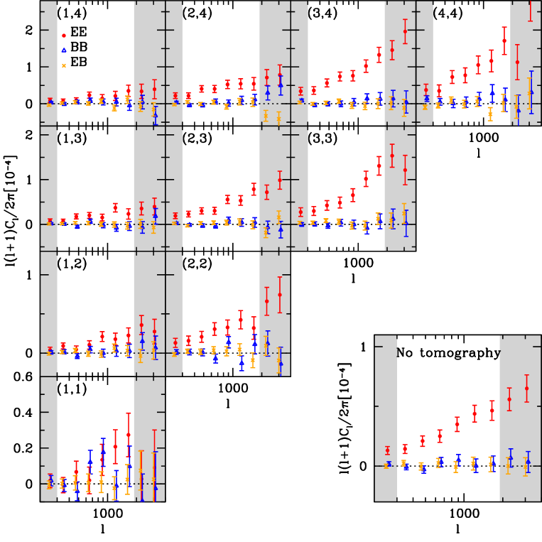
Figure 1: Tomographic cosmic shear power spectra of EE (red filled circles), BB (blue open triangles), and EB (yellow crosses) modes. The galaxy samples are divided into four tomographic redshift bins using the Ephor AB photo-$z$ code. The redshift ranges of the four tomographic bins are set to [$0.3$, $0.6$], [$0.6$, $0.9$], [$0.9$, $1.2$], and [$1.2$,$1.5$], for binning number 1 to 4 (see also Table 1). The right-bottom panel shows the non-tomographic cosmic shear power spectrum. The multipole ranges of $\ell<300$ and $\ell>1900$ (shaded regions) are excluded in the cosmological analysis. The combined total detection significance of the tomographic EE-auto spectra is $16\sigma$ in the range of $300<\ell<1900$ (unshaded regions), whereas both BB and EB-mode spectra are consistent with zero.

3 Measurement methods

In this section, we summarize the measurement of cosmic shear power spectra using the pseudo-$C_{\ell}$ method. More details of the formulation and validation tests using mock shear catalogs are given in Appendix A. We also present the blinding methodology adopted throughout our analysis.

3.1 Pseudo-$C_{\ell}$ method

We characterize cosmic shear signals using the power spectrum defined in Fourier space. The power spectrum, which is the mean square of fluctuation amplitudes as a function of wavenumber $k$, or multipole $\ell$, is one of the most fundamental statistics to describe the clustering properties of density fields (e.g., Tegmark et al., 2004). The power spectrum has been measured from different probes of the cosmic density fields including CMB (e.g., Hinshaw et al., 2013; Planck Collaboration et al., 2016), the distribution of galaxies (e.g., Cole et al., 2005; Yamamoto et al., 2006; Percival et al., 2010; Reid et al., 2010; Blake et al., 2011; Oka et al., 2014; Alam et al., 2017; Beutler et al., 2017), and the Lyman-$\alpha$ forest (e.g., McDonald et al., 2006; Palanque-Delabrouille et al., 2013; Viel et al., 2013; Iršič et al., 2017).

However, it is non-trivial to measure the power spectrum in an unbiased manner from data with incomplete sky coverage. In weak lensing surveys, the sky coverage is usually very non-uniform due to complicated survey geometry resulting from bright star masks, survey boundaries, non-uniform survey depths, and non-uniform galaxy shape weights. The observed shear field is given by the weighted sum of shear values over galaxies in each sky pixel as

$$\bm{\gamma}^{\rm(obs)}(\bm{\theta})=W(\bm{\theta})\bm{\gamma}^{\rm(true)}(\bm{\theta}),$$ (7)

where $W({\bm{\theta}})$ represents the survey window defined as the sum of shear weights in each pixel. When a sky position ${\bm{\theta}}$ is outside the survey area or masked due to a bright star, $W({\bm{\theta}})$ is set to zero. We define a rectangular-shape region enclosing each of the six HSC patches and then perform the Fourier transformation of the observed shear field, $\bm{\gamma}^{\rm obs}$, with typical pixel scale of about 0.88 arcmin, which is much smaller than the scales we use in our cosmological analysis. The power spectrum obtained simply from the amplitude of the Fourier-transformed shear field is biased due to the convolution with the mask field $W$. We apply the pseudo-$C_{\ell}$ method to obtain unbiased estimates of the cosmic shear power spectrum by correcting for the convolution with the survey window (Hikage et al., 2011; Kitching et al., 2012; Hikage & Oguri, 2016; Asgari et al., 2018). This method has also been commonly used in CMB analyses (Kogut et al., 2003; Brown et al., 2005). The details of the method may be found in Appendix A. In short, the dimensionless binned lensing power spectrum ${\cal C}_{b}^{\rm(true)}$ corrected for the masking effect is given by

$${\cal C}_{b}^{\rm(true)}=\bm{M}_{bb^{\prime}}^{-1}\sum_{\bm{\ell}}^{|{\bm{\ell}}|\in\ell_{b}^{\prime}}P_{b^{\prime}\ell}(\bm{C}_{\bm{\ell}}^{\rm(obs)}-\langle\bm{N}_{\bm{\ell}}\rangle_{\rm MC}),$$ (8)

where $\bm{M}_{bb^{\prime}}$ is the mode coupling matrix of binned spectra, which is related to the survey window $W$ by equation (52), $\bm{C}_{\bm{\ell}}^{\rm(obs)}$ is the pseudo-spectrum (masked spectrum) that we can directly measure from the Fourier transform of ${\bf\gamma}^{\rm obs}$, and $P_{b\ell}=\ell^{2}/2\pi$ is a conversion factor to the dimensionless power spectrum. The sum is over all Fourier modes in the given $\ell$ bin ($\ell_{b}^{\prime}$). In order to remove the shot noise, we randomly rotate orientations of individual galaxies to estimate the shot noise power spectrum $\bm{N}_{\bm{\ell}}$, and subtract it from $\bm{C}_{\bm{\ell}}^{\rm(obs)}$. Specifically, we use 10000 Monte Carlo simulations with random galaxy orientations to estimate the convolved noise spectrum $\langle{\bm{N}}_{\ell}\rangle_{\rm MC}$. We use 15 logarithmically equal bins in the range $60\leq\ell\leq 6500$, although we restrict ourselves to a narrower range for our cosmological inferences.

While the validity and accuracy of our pseudo-$C_{\ell}$ method have been studied in depth in previous work (Hikage et al., 2011; Hikage & Oguri, 2016), we explicitly check the accuracy of the pseudo-$C_{\ell}$ method for the HSC first-year shear catalog by applying the method to the HSC mock shear catalogs presented in Oguri et al. (2018). Note that this mock test is for verifying that our pseudo-$C_{\ell}$ method produces the unbiased measurement of lensing power spectra from inhomogeneous shear data, but not for verifying our modeling such as intrinsic alignment and baryon feedback. The mock shear catalogs have the same survey geometry and spatial inhomogeneity as the real HSC first-year data, and include random realizations of cosmic shear from the all-sky ray-tracing simulation presented in Takahashi et al. (2017). These realistic mock catalogs allow us to check the accuracy of the pseudo-$C_{\ell}$ method in correcting for the masking effect, as well as the accuracy of our analytic estimate of the covariance matrix as we will discuss below. The results of the test with the HSC mock shear catalogs are also presented in Appendix A. We find that our pseudo-$C_{\ell}$ method recovers the input cosmic shear power spectrum within 10% of the current statistical errors at least over the range of $\ell$ of interest, $80<\ell<2000$. We also confirm that the input values of $\Omega_{\rm m}$, $\sigma_{8}$, and $S_{8}$ are successfully recovered from the mock catalogs. Specifically, from the analysis of the mock catalogs we obtain $\Omega_{\rm m}=0.292\pm 0.014$, $\sigma_{8}=0.801\pm 0.020$, and $S_{8}=0.791\pm 0.005$, which are consistent with the input values, $\Omega_{\rm m}=0.279$, $\sigma_{8}=0.82$, and $S_{8}=0.791$ to within the 68% credible interval. The credible intervals (error bars) are roughly $1/\sqrt{100}$ of the accuracy we can achieve with the HSC first year shear catalog.

We note that the cosmic shear (E-mode) power spectrum is related to the shear correlation functions $\xi_{+}$ and $\xi_{-}$ as

$$\xi_{\pm}(\theta)=\frac{1}{2\pi}\int d\ell\,\ell~{}C_{\ell}J_{0,4}(\ell\theta),$$ (9)

where $J_{n}(x)$ is the $n$-th order Bessel function of the first kind. While mathematically the cosmic shear power spectrum carries the same information as the shear two-point correlation functions for a full-sky uniform survey, this is not exactly true in finite-sky data. In addition, the covariance of the power spectrum is diagonal in Gaussian fields, whereas the covariance of the two-point correlation functions contains significant non-diagonal elements even for Gaussian fields. Since the Gaussian error still dominates in the current cosmic shear measurements, the statistical independence is high among different $\ell$ modes.

3.2 Blinding

We have entered an era of precision cosmology. With a growing number of cosmological probes, one has to carefully guard against biases, including confirmation bias, which may be particularly relevant when comparing results with other experiments. To avoid confirmation bias, we perform our cosmological analysis in a blind fashion. Within the HSC team, there are multiple projects performing cosmological analysis on the weak lensing data, each with separate individual timelines. Therefore we pursue a two-tiered blinding strategy such that unblinding one of the analysis teams does not automatically unblind the others. First, each analysis team is blinded separately at the catalog level by preparing a set of three shear catalogs per analysis team with different values of the multiplicative bias such that

$${\bf m}^{i}_{\rm cat}={\bf m}_{\rm true}+\mathrm{d}{\bf m}^{i}_{1}+\mathrm{d}{\bf m}^{i}_{2}\,,$$ (10)

where ${\bf m}_{\rm true}$ denotes the array of multiplicative bias values for HSC galaxies as estimated in simulations and the index $i$ runs from 0 to 2 and denotes the three different shear catalog versions. The terms $\mathrm{d}{\bf m}^{i}_{1}$ and $\mathrm{d}{\bf m}^{i}_{2}$ are different for each of three catalogs sent to each analysis team. The values of each of these terms are stored in an encrypted manner in the headers of the three shear catalogs. The term $\mathrm{d}{\bf m}^{i}_{1}$ can only be decrypted by the analysis team lead, and this term is removed before performing the analysis. The term $\mathrm{d}{\bf m}^{i}_{2}$ can only be decrypted by the blinder-in-chief once the encrypted headers for $\mathrm{d}{\bf m}^{i}_{2}$ (stored in the shear catalog) are passed on by the analysis team. Exactly one of the three values among $\mathrm{d}{\bf m}^{i}_{2}$ is zero, and can be revealed by the blinder-in-chief once the analysis team is ready for unblinding. The blinder-in-chief does not play any active role in the cosmological analysis and is her/himself not aware of the values of $\mathrm{d}{\bf m}^{i}_{2}$ until the end. The analysis group thus has to perform 3 analyses, a costly enterprise, but then it avoids the need for reanalysis once the catalogs are unblinded.

The presence of $\mathrm{d}{\bf m}^{i}_{1}$ prevents accidental unblinding by comparison of two sets of blinded catalogs sent out to two different analysis teams. The presence of separate $\mathrm{d}{\bf m}^{i}_{2}$ allows each analysis team to remain blinded separately from the other analysis teams. This constitutes the first tier of our blinding strategy. The different multiplicative biases result in a similar shape for the cosmic shear power spectra, but different overall amplitudes, and thus different values of $S_{8}$. The values of $\mathrm{d}{\bf m}^{i}_{2}$ are drawn randomly to allow variations in $S_{8}$ at levels comparable to the differences between the $S_{8}$ values inferred by Planck and other contemporary lensing surveys.

We also guard ourselves against the possibility that the values of $\mathrm{d}{\bf m}^{i}_{2}$ all come out close to each other by chance. This would automatically result in unblinding if we compared our cosmological constraints to other surveys. Therefore as a second tier of protection, we also remain blinded at the analysis level. We never compare the cosmic shear power spectra obtained from any of our blinded catalogs with any theoretical predictions on plots where the cosmological parameters of the predictions were known beforehand. In addition, prior to unblinding we always plot our cosmological constraints with the mean values subtracted off and thus centered at zero. Moreover, we do not compare our cosmological constraints, even after shifting by the mean values, with constraints from other surveys and experiments.

Prior to the start of the analysis we set down the conditions that must be satisfied and systematics tests to be carried out before unblinding. The first set of these conditions includes sanity checks about the satisfactory convergence of posterior distributions on cosmological parameters for each of the three shear catalogs given to the analysis team (see Appendix C). The second set concerns the analysis choices for cosmic shear and study of their impact on the cosmological constraints. These conditions were as follows:

• Make the code available to all collaboration members. Specific people were assigned to review the code.

• Test that the measurement code can recover the input power spectrum from a mock data set within statistical uncertainties.

• Test that the inference code can recover cosmological parameters, in particular $S_{8}$, from the cosmic shear signal inferred from a mock dataset within statistical uncertainties.

• Estimate the systematic uncertainty due to the differences between various photo-$z$ estimates, and quantify impact on the cosmological constraints.

• Quantify the impact of the range of angular scales used, in particular whether dropping the smaller angular scales results in a statistically significant change to the inferred cosmological constraints.

• Quantify the impact of removing individual photometric redshift bins from the analysis and test whether any specific bins result in a statistically significant shift of parameters.

• Test the goodness of fit for the measured cosmic shear power spectra from all of the blinded catalogs.

• Quantify the impact of using different sets of matter power spectra obtained from numerical simulations with a variation in the baryonic physics recipes.

This paper describes the results of most of these tests. Once a decision to unblind is reached, the second tier of blinding (analysis level blinding) is removed by the analysis team just a few hours prior to the final unblinding by the blinder-in-chief. Plots with cosmological constraints and their comparison with the CMB results are made for each of the three catalogs. The encrypted headers with values of $\mathrm{d}{\bf m}^{i}_{2}$ are sent to the blinder-in-chief so that the blinder-in-chief can decrypt these values and give them to the analysis team.

Lastly, we emphasize that we started our cosmological analysis only after the HSC first year shear catalog (Mandelbaum et al., 2018a) was finalized, i.e., the construction of the shear catalog was not influenced by the cosmic shear signal, its shape or amplitude. Although the shear catalog and the associated systematic tests were finalized without blinding, the cosmological analysis does not influence the decisions related to the shear catalog.

4 Cosmic shear measurement

In this section, we present the measurement of tomographic cosmic shear power spectra using the HSC first year shear catalog by separating their E-mode and B-mode signals. We also estimate the impact of PSF leakage and residual PSF model errors on our cosmic shear measurement.

4.1 Cosmic shear power spectra

We use the pseudo-$C_{\ell}$ method described in Section 3.1 to measure tomographic cosmic shear power spectra of E-mode, B-mode auto, and EB-cross modes from the HSC first-year shear catalog. The power spectra are shown in Figure 1. In deriving the spectra, we first measured cosmic shear spectra in the six disjoint fields individually, and then obtained a weighted average of the spectra using weights computed from the sum of source weights of individual galaxies, $w_{i}$ (equation 4).

We find that the B-mode signals appear qualitatively consistent with zero, as expected. A possible exception is in the low multipole range $\ell<300$, where the excess B-mode signals are significant. As Oguri et al. (2018) found 2-3$\sigma$ B-mode residuals due to PSF modeling errors, this is partly due to the PSF model ellipticity residuals, as we will discuss in Section 4.2. Therefore, in our cosmic shear analysis, we set the lower limit of the multipoles to $\ell_{\rm min}=300$. We also set the upper limit to $\ell_{\rm max}=1900$ because of model uncertainties at such high multipole, as we will discuss in Section 5. As shown by Asgari et al. (2018), removing scales with significant B-modes does not always ensure that the systematic error that causes those B-modes does not impact the E-modes on other scales. To further mitigate the systematic effect, we take account of both PSF leakage and residual PSF model errors in our modeling, although their contribution is small on the fiducial range of scales (see Section 5.6).

We quantitatively check the consistency of the B-mode cosmic shear power spectra with zero using the following chi-squared statistic,

$$\chi^{2}=\sum_{i,j,i^{\prime},j^{\prime}}\sum_{b,b^{\prime}}^{\ell_{\rm min}\leq\ell_{b}\leq\ell_{\rm max}}C_{b}^{BB(ij)}({\cal N}^{BB})^{-1}_{bb^{\prime}}C_{b^{\prime}}^{BB(i^{\prime}j^{\prime})}\,,$$ (11)

where the first summation runs over the four tomographic bins. For the covariance of the B-mode cosmic shear power spectra, we only use the shape noise covariance ${\cal N}^{BB}$. While it is often assumed that the shape noise covariance is given by a simple analytic expression that depends only on the dispersion of galaxy ellipticities and the number density of galaxies, in real observations various effects such as the survey window function and the inhomogeneous distribution of galaxies modify the shape noise covariance (e.g., Murata et al., 2018; Troxel et al., 2018b). In order to obtain an accurate shape noise covariance, we estimate the covariance directly from the data, based on the estimate of the average shot noise power spectrum discussed in Section 3.1 in which we randomly rotate the orientations of source galaxies 10,000 times. From this Monte Carlo sampling of shape noise power spectra, we can directly construct the covariance matrix of shape noise power spectra corrected for masking effects. We use this noise covariance matrix throughout the paper. This noise covariance matrix is mostly diagonal, but we find non-zero ($\lesssim 20\%$) off-diagonal components mostly between neighboring multipole bins, which we also include in our analysis.

We find no significant B-mode signal for any of the auto- and cross-power spectra measured between our fiducial four tomographic bins. The most significant deviation from zero is found in the lowest-redshift auto tomographic bin for which we find $\chi^{2}=12.1$ with $6$ data points, resulting in a $p$-value of 0.06. The total $\chi^{2}$ over four bin tomographic B-mode auto spectra becomes 60.7 with $60$ data points of the B-mode spectra (the resulting $p$-value of 0.45) for our fiducial choice of $300<\ell<1900$. For the EB-cross mode, $\chi^{2}=59.7$ with the same 60 data points (with a resulting $p$-value of 0.49). We also confirm that there are no significant B-mode signals even if we adopt other photo-$z$ codes. We see no evidence either for systematics in the data producing B-modes, or for leakage of E-mode power into B-mode power due to the convolution of survey masks. The latter indicates that our pseudo-$C_{\ell}$ method successfully decomposes E- and B-modes as expected from the analysis using HSC mock shear catalogs presented in Appendix A.

4.2 PSF leakage and residual PSF model errors

Systematics tests of the HSC first-year shear catalog presented in Mandelbaum et al. (2018a) and Oguri et al. (2018) indicate that there are small residual correlations between galaxy ellipticities and PSF ellipticities resulting from imperfect PSF corrections. Such residual PSF model errors could produce artificial two-point correlations and hence bias our cosmic shear results. We check the impact of these systematics in our cosmic shear measurements assuming that the measured galaxy shapes have an additional additive bias given by

$$e^{\rm(sys)}=\tilde{\alpha}e^{\rm p}+\tilde{\beta}e^{\rm q}.$$ (12)

The first term in the right hand side, referred to as PSF leakage, represents the systematic error proportional to the PSF model ellipticity $e^{\rm p}$ due to the deconvolution errors of the PSF model. The second term represents the systematic error associated with the difference between the model PSF ellipticity, $e^{\rm p}$, and the true PSF ellipticity that is estimated from individual “reserved” stars, $e^{\rm star}$, i.e., $e^{\rm q}\equiv e^{\rm p}-e^{\rm star}$ (Troxel et al., 2018a). The non-zero residual PSF ellipticity $e^{\rm q}$ indicates an imperfect PSF estimate, which should also propagate to shear estimates for galaxies. While the systematics tests carried out by Mandelbaum et al. (2018a) and Oguri et al. (2018) suggest that these PSF leakage and residual PSF model errors do not significantly affect our cosmological analysis, it is of great importance to directly check the potential impact of these errors on our measurements of the cosmic shear power spectra.

When $e^{\rm(sys)}$ [equation (12)] is added to the observed galaxy ellipticity, these systematic terms change the measured cosmic shear power spectrum as

$$C_{\ell} \rightarrow C_{\ell}+\tilde{\alpha}^{2}C_{\ell}^{\rm pp}+2\tilde{\alpha}\tilde{\beta}C_{\ell}^{\rm pq}+\tilde{\beta}^{2}C_{\ell}^{\rm qq}\,,$$ (13)

where $C_{\ell}^{\rm pp}$, $C_{\ell}^{\rm qq}$, and $C_{\ell}^{\rm pq}$ represent the auto-spectrum of the model ellipticity $e_{\rm p}$, the auto-spectrum of the residual PSF ellipticity $e_{\rm q}$, and the cross-spectrum of $e_{\rm p}$ and $e_{\rm q}$, respectively. We subtract the shot noise term in the calculation of $C_{\ell}^{\rm pp}$ and $C_{\ell}^{\rm qq}$, which means that these power spectra would be zero if there were no spatial correlation in $e_{\rm p}$ and $e_{\rm q}$, and that the value of the power spectrum shown on the plots cannot be simply related to the typical PSF ellipticity value. The proportionality factors $\tilde{\alpha}$ and $\tilde{\beta}$ are measured by cross-correlating $e^{\rm p}$ and $e^{\rm q}$ with the observed galaxy ellipticities as

$$C_{\ell}^{\rm gp} = \tilde{\alpha}C_{\ell}^{\rm pp}+\tilde{\beta}C_{\ell}^{\rm pq}\,,$$ (14)

$$C_{\ell}^{\rm gq} = \tilde{\alpha}C_{\ell}^{\rm pq}+\tilde{\beta}C_{\ell}^{\rm qq}\,,$$ (15)

where $C_{\ell}^{\rm gp}$ and $C_{\ell}^{\rm gq}$ denote the cross-spectra between galaxy ellipticities used for the cosmic shear analysis and $e_{\rm p}$ and $e_{\rm q}$, respectively.

In the HSC software pipeline (Bosch et al., 2018), PSF stars are selected based on the distribution of high-$S/N$ objects with size. However, $\sim 20\%$ of such stars are not used for PSF modeling, so that they can be used for cross-validation of PSF modeling. This $\sim 20\%$ sample of stars is referred to here as the reserved star sample. In this paper, we use this subsample of stars for computing the auto- and cross-spectra of $e_{\rm p}$ and $e_{\rm q}$ (Figure 2). Using equations (14) and (15), we find $\tilde{\alpha}=0.057\pm 0.018$ and $\tilde{\beta}=-1.22\pm 0.74$, where the errors are estimated by randomly rotating orientations of the stars.

Given that the systematics in galaxy shape measurements depend only upon the shapes and brightness of galaxies and not directly upon their redshifts, per se, as a first order approximation, it is reasonable to assume that $\tilde{\alpha}$ and $\tilde{\beta}$ are common for all tomographic bins. However, it is plausible that the values of $\tilde{\alpha}$ and $\tilde{\beta}$ are slightly different for different tomographic bins, reflecting the different distributions of galaxy properties such as their sizes and $S/N$ ratio. In particular, the impact of PSF model shape errors on the shear two-point correlations depends on the size distribution of the galaxies compared to the PSF, which we call “resolution” (see, e.g., Section 3.4 of Jarvis et al., 2016). Therefore, we compare the distribution of resolution factors among the four tomographic bins, and find that both mean values and overall distributions of resolution factors are very similar among the four tomographic bins. Specifically, the weighted mean values of the resolution factor $R_{2}$ are 0.603, 0.592, 0.598, and 0.596 from lowest to highest redshift bins (see also Mandelbaum et al., 2018b). This suggests that the redshift dependence of $\tilde{\beta}$ coming from the difference of galaxy sizes is negligibly small. We also note that, even if small redshift dependences of $\tilde{\alpha}$ and $\tilde{\beta}$ are present, the values between the different tomographic bins would be highly correlated. Given that the number of the reserved stars is modest, the estimates of $\tilde{\alpha}$ and $\tilde{\beta}$ from the auto- and cross-correlation analysis is noisy by nature, making it challenging to estimate these values for individual tomographic bins as well as their covariance between different tomographic bins. For these reasons, we adopt the common values of $\tilde{\alpha}$ and $\tilde{\beta}$ found above for all the tomographic bins as our estimates of systematics from the PSF leakage and PSF model residuals.

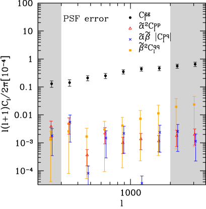
Figure 2: The auto power spectrum of the PSF leakage $\tilde{\alpha}^{2}C_{\ell}^{pp}$ (open triangles), that of the residual PSF $\tilde{\beta}^{2}C_{\ell}^{qq}$ (filled squares), and their cross-spectrum $\tilde{\alpha}\tilde{\beta}|C_{\ell}^{pq}|$ (crosses) are compared with the non-tomographic cosmic shear power spectrum $C^{\rm gg}_{\ell}$ (filled circles) (see Section 4.2 for details). The shaded region indicates the range of multipoles that is excluded in our fiducial cosmological analysis. It is found that both of the PSF systematics are subdominant in the fiducial multipole range.

Figure 2 shows the auto spectra of the PSF leakage and residual PSF model errors as well as their cross spectra. We find that both the PSF systematics are subdominant and the amplitudes of the power spectra of both the PSF systematics are less than 5% of the non-tomographic cosmic shear power spectrum over our fiducial range of scales. Although the contribution of the PSF systematics to the total cosmic shear power spectrum is not very significant, it could represent a larger fraction of the tomographic cosmic shear power spectra in low redshift bins. Therefore, in our cosmological analysis, we marginalize over the PSF systematics by introducing two nuisance parameters $\tilde{\alpha}$ and $\tilde{\beta}$ with Gaussian priors as obtained from our systematics analysis.

We note that the mean shear value of the HSC first-year shear catalog, $\langle{\bf\gamma}^{\rm obs}\rangle$, is consistent with zero, as can be seen from the comparison of the data with the HSC mock shear catalogs that include cosmic variance (Mandelbaum et al., 2018a; Oguri et al., 2018). We do not subtract the mean shear value from the shear catalog because such subtraction would artificially suppress the cosmic shear power especially at small $\ell$ where the small sky coverage gives a limited number of modes.

5 Model ingredients for cosmological analysis

In this section, we summarize our model for the measured cosmic shear power spectra which we use for the cosmology analysis. In addition to the cosmic shear signal, our model accounts for various astrophysical effects such as the intrinsic alignment of galaxies and the impact of baryon physics as well as systematics due to photo-$z$ and shape measurement uncertainties. We also describe our analytical estimate of the covariance matrix. We summarize the parameters of our fiducial cosmological model as well as nuisance parameters and their priors that we use in our analysis.

5.1 Cosmic shear signals

The comparison of observed cosmic shear power spectra derived in Section 4.1 with model-predicted power spectra allows us to constrain cosmological parameters. In particular adding redshift information of source galaxies into the cosmic shear measurements, the so-called cosmic shear tomography (Hu, 1999; Takada & Jain, 2004), enables us to improve the cosmological constraints by lifting degeneracies among parameters. We compute cosmic shear power spectra for arbitrary cosmological models using the flat-sky and Limber approximations (see Kitching et al., 2017; Kilbinger et al., 2017, for the validity of these approximations in our study) such that

$$C_{\ell}^{(ij)}=\int_{0}^{\chi_{H}}d\chi\frac{q^{(i)}(\chi)q^{(j)}(\chi)}{f_{K}^{2}(\chi)}P_{\rm mm}^{\rm NL}\left(k=\frac{\ell+1/2}{f_{K}(\chi)},z\right),$$ (16)

where $i$ and $j$ refer to tomographic bins, $\chi$ is the comoving radial distance, $\chi_{H}$ is the comoving horizon distance and $f_{\rm K}(\chi)$ is the comoving angular diameter distance. As our fiducial model, we use the fitting formula for the nonlinear matter power spectrum $P_{\rm mm}^{\rm NL}(k,z)$ provided by Takahashi et al. (2012), which is an improved version of the halofit model by Smith et al. (2003) (see also Section 5.5). We use this improved halofit model implemented in Monte Python (Audren et al., 2013) which adopts the Boltzmann code CLASS to compute the evolution of linear matter perturbations (Lesgourgues, 2011; Audren & Lesgourgues, 2011; Blas et al., 2011). While we do not include neutrino mass in our fiducial analysis, we also check the effect of a non-zero neutrino mass by replacing the halofit model of Takahashi et al. (2012) with that of Bird et al. (2012).

The lensing efficiency function $q^{(i)}(\chi)$ for the $i$-th tomographic bin is defined as

$$q^{(i)}(\chi) \equiv \frac{3}{2}\Omega_{\rm m}H_{0}^{2}\int_{\chi}^{\chi_{H}}d\chi^{\prime}p^{(i)}(\chi^{\prime})(1+z)\frac{f_{K}(\chi)f_{K}(\chi,\chi^{\prime})}{f_{K}(\chi^{\prime})},$$

where $p^{(i)}(\chi)$ denotes the redshift distribution of source galaxies in the $i$-th tomographic bin and is normalized such that $\int d\chi^{\prime}p^{(i)}(\chi^{\prime})=1$.

5.2 Source redshift distributions

We infer the source redshift distributions in individual tomographic bins, $\bar{P}^{(i)}(z)\equiv(d\chi/dz)p^{(i)}(\chi)$, based on the broadband photometry of the HSC survey. In order to estimate the redshift distribution of the source galaxies, we would ideally obtain spectroscopic redshifts for a representative subsample of galaxies in our sample. Given the depth of the HSC survey ($i<24.5$), this is quite a challenging task. There are a number of spectroscopic redshift (spec-$z$ hereafter) surveys that overlap with the HSC footprint, such as GAMA (Liske et al., 2015) and VVDS (Le Fèvre et al., 2013). The differences between the populations of these existing spec-$z$ samples and the weak lensing source galaxy sample could potentially be accounted for by using clustering and reweighting techniques (see Bonnett et al., 2016; Gruen & Brimioulle, 2017, for assumptions and caveats of this method). These methods place galaxies in the source galaxy sample into groups with similar photometric properties. Galaxies from the spectroscopic sample that belong to the same groups are reweighted to mimic the distribution of the weak lensing source galaxy sample (Lima et al., 2008). Unfortunately, the number of galaxies in the spectroscopic samples is not large enough to accurately represent the photometric properties of our source sample even after reweighting.

Therefore, instead of the spec-$z$ sample, we use the 2016 version of the COSMOS 30-band photo-$z$ catalog (Ilbert et al., 2009; Laigle et al., 2016) and accept it as the ground truth. There are a number of caveats that come with this assumption. First, the COSMOS sample represents a small area of the sky and could be affected by sample variance. Secondly, the photometric redshift codes used in the HSC survey have been trained on the COSMOS 30-band photo-$z$ sample (see Tanaka et al., 2018), which could lead to some circularity in logic. Thirdly, even though COSMOS photo-$z$’s use 30-band information, they are not as good as having spectroscopic redshifts. For example, COSMOS photo-$z$’s are known to have attractor solutions which could cause unnecessary pile up of photo-$z$’s at certain locations in photo-$z$ space (see also discussions in Tanaka et al., 2018).

The reweighting method can overcome sample variance to some extent, as it determines appropriate weights to map the COSMOS 30-band photo-$z$ sample to the HSC weak lensing sample that we use in our analysis. This relies on the assumption that the color-redshift relation does not vary with environment (Hogg et al., 2004; Gruen & Brimioulle, 2017). Based on the variance of the four CFHTLS deep fields, Gruen & Brimioulle (2017) estimated the cosmic variance contribution in the context of galaxy-galaxy lensing and found the effect on the angular diameter distance ratios in lensing to be approximately 3% of the lens redshifts. Unfortunately only two of these fields are in the current HSC footprint, which makes it difficult to compute similar estimates of cosmic variance for our cosmic shear results. The other way to estimate the cosmic variance would be to populate mock simulation catalogs with galaxies with appropriate spectral energy distributions (Hoyle et al., 2018). The algorithms to achieve an appropriate assignment of HSC colors to the galaxies based on environment and its evolution with redshift is still a subject of active research.

As a workaround to the second caveat, we reserved 20$\%$ of the galaxies from the original COSMOS 30-band photo-$z$ catalog, which are not used for training the HSC photo-$z$’s. We use this subsample for testing purposes. In the future, to avoid the photo-$z$ issues, we plan to make use of the cross-correlation technique to obtain clustering redshifts (Newman, 2008; Ménard et al., 2013; McQuinn & White, 2013). Unfortunately, the area covered in the current data release is not large enough to apply this method. Therefore, we use the COSMOS reweighted distribution as our fiducial choice, but use the stacked photo-$z$ PDFs to propagate our uncertain knowledge of the redshift distributions to our cosmological constraints.

Here we describe our procedure to obtain the weights that map the COSMOS 30-band photo-$z$ sample to the HSC weak lensing sample. For this purpose, we employ the HSC Wide observation of the COSMOS field, although it is not included in our HSC first year shear catalog presented in Mandelbaum et al. (2018a). The HSC $i$-band images in the COSMOS field, which were obtained in the same observing constraints as the HSC Wide survey overall, allows us to obtain weak lensing weights [equation (4)] for each of the COSMOS galaxies, as well as the photo-$z$ as inferred by our different pipelines exclusively based on the HSC photometry. We only use those COSMOS galaxies which also pass our weak lensing cuts.

We first sort the galaxies in our entire weak lensing shear catalog using their $i$-band cmodel magnitude and 4 colors (based on the afterburner photometry) into cells of a self-organizing map (SOM; More et al., in prep.). The self-organizing map is a clustering technique which groups objects of similar properties together (see Masters et al., 2015, for application to photometric redshifts). Given the HSC photometry, we classify the COSMOS galaxies into SOM cells defined by the source galaxy sample. We then compute weights for galaxies that belong to each SOM cell ($w^{i}_{\rm SOM}$) such that

$$w^{i}_{\rm SOM}=\frac{N_{\rm wl}^{i}}{N_{\rm COSMOS}^{i}}$$ (18)

where $N_{\rm wl}^{i}$ denotes the number of galaxies in the weak lensing source galaxy sample in the $i^{\rm th}$ cell, and $N_{\rm COSMOS}^{i}$ denotes the number of galaxies in the COSMOS galaxy sample. The weighted COSMOS 30-band photo-$z$ sample thus mimics our source galaxy sample in terms of the photometry. We do not account for the errors in the HSC photometry as the errors are the same for the HSC weak lensing sample and the COSMOS photo-$z$ sample (Gruen & Brimioulle, 2017).

In order to compute the redshift distribution of the sources in the four different redshift bins of our weak lensing shear catalog, we mimic our selection criteria on the COSMOS 30-band sample, using HSC photometry and the HSC-derived photometric redshifts ($z_{\rm best}$) from the Ephor AB pipeline, which is the code we used to define the tomographic bins. Given these samples, we infer the redshift distribution as a histogram of COSMOS 30-band photo-$z$ weighted by the lensing source weights times the SOM weights. In order to compute the statistical noise due to the limited number of COSMOS galaxies lying in certain SOM bins, we also perform a jackknife estimate of the statistical error on the $P(z)$ distribution using 10 jackknife samples of the COSMOS galaxies.

On the other hand, the stacked photo-$z$ PDFs from the different HSC photo-$z$ codes are derived by stacking the full PDF of photo-$z$’s for individual galaxies $P_{j}(z)$ with their weight $w_{j}$ [equation (4)]

$$\bar{P}^{(i)}(z)=\frac{\sum_{j}^{z_{\rm min}^{(i)}<z_{j}^{\rm best}<z_{\rm max}^{(i)}}w_{j}P_{j}(z)}{\sum_{j}^{z_{\rm min}^{(i)}<z_{j}^{\rm best}<z_{\rm max}^{(i)}}w_{j}}.$$ (19)

We note that $\bar{P}^{(i)}(z)$ estimated by COSMOS-reweighted or stacked PDF of photo-$z$s has tails that extend beyond the tomographic bin range $z_{\rm min}^{(i)}<z<z_{\rm max}^{(i)}$ simply because of the finite width in the $P^{(i)}(z)$ of all galaxies.

We adopt the COSMOS-reweighted redshift distribution as our fiducial choice for the redshift distributions. To be conservative, we allow these redshift distributions to shift in the redshift direction by an amount $\Delta z$ in each bin, independently, which result in a corresponding shift to the means of the redshift distribution. We use the differences between the COSMOS reweighted photo-$z$’s and the stacked photo-$z$ PDFs to put priors on $\Delta z$ and propagate our uncertain knowledge of the redshift distributions to our cosmological constraints (see Section 5.8).

5.3 Covariance

Accurate covariance matrices are crucial to make a robust estimation of cosmological parameters from the measured cosmic shear power spectra. Without loss of generality we can break down the covariance matrix of cosmic shear power spectra into three parts:

$${\rm Cov}^{\rm(tot)}={\rm Cov}^{\rm(G)}+{\rm Cov}^{\rm(NG)}+{\rm Cov}^{\rm(SSC)},$$ (20)

where ${\rm Cov}^{\rm(G)}$, ${\rm Cov}^{\rm(NG)}$, and ${\rm Cov}^{\rm(SSC)}$ denote the Gaussian (G), the non-Gaussian (NG), and the super-sample covariance (SSC) contribution to the covariance, respectively. As discussed in Appendix B, we adopt an analytical halo model for computing the covariance (Cooray & Sheth, 2002), except that we use the direct estimate of the shape noise covariance, ${\cal N}^{BB}_{bb^{\prime}}$ [see around equation (11)]. The shape noise covariance is one part of ${\rm Cov}^{\rm(G)}$ [see equation (66) in Appendix B].

The Gaussian and non-Gaussian power spectrum covariances have been well studied in previous work (Scoccimarro et al., 1999; Takada & Jain, 2009). The excess covariance due to super-sample modes has also been studied (Takada & Bridle, 2007; Takada & Jain, 2009; Takada & Hu, 2013) and tested using ray-tracing simulations (Sato et al., 2009). Based on these findings, we employ an analytical halo model to compute the sample variance contribution. Our analytic model of covariance includes all these components, as well as its cosmological dependence. While the analytic model involves various approximations, we show in Appendix B that it agrees well with the covariance matrix estimated using the HSC mock shear catalogs.

5.4 Intrinsic alignment

One of the major astrophysical systematic effects in the cosmic shear analysis is the intrinsic alignment (IA) of galaxy shapes (see Joachimi et al., 2015; Kirk et al., 2015; Kiessling et al., 2015, for recent reviews). The intrinsic alignment comes from two contributions. One is the correlation between the intrinsic shapes of two galaxies residing in the same local field (Heavens et al., 2000; Croft & Metzler, 2000; Lee & Pen, 2000; Catelan et al., 2001). The other is the correlation of the gravitational shear acting on one galaxy and the intrinsic shape of another galaxy (Hirata & Seljak, 2004).

In this paper we adopt a nonlinear alignment (NLA) model (Bridle & King, 2007), which is commonly used in cosmic shear analysis, to describe the IA contributions. The NLA model is based on the linear alignment model (Hirata & Seljak, 2004), but the linear matter power spectrum is replaced with the nonlinear power spectrum. This phenomenological model has been found to fit the galaxy-shear cross correlations down to $\lower 2.15277pt\hbox{$\;\buildrel>\over{\sim}\;$}1-2h^{-1}$Mpc quite well (Singh et al., 2015; Blazek et al., 2015), and has been used in various cosmic shear analyses (Heymans et al., 2013; Kitching et al., 2014; Abbott et al., 2016; Hildebrandt et al., 2017). In this model, the intrinsic-intrinsic (II) and shear-intrinsic (GI) power spectra are given by

$$P_{\rm II}(k,z) = F^{2}(z)P_{\rm mm}^{\rm NL}(k,z),$$ (21)

$$P_{\rm GI}(k,z) = F(z)P_{\rm mm}^{\rm NL}(k,z).$$ (22)

The redshift- and cosmology-dependent factor relating the galaxy ellipticity and the gravitational tidal field is often parametrized as

$$F(z)=-A_{\rm IA}C_{1}\rho_{\rm crit,0}\frac{\Omega_{\rm m}}{D(z)}\left(\frac{1+z}{1+z_{0}}\right)^{\eta}\left(\frac{\bar{L}(z)}{L_{0}}\right)^{\beta},$$ (23)

where $A_{\rm IA}$ is a dimensionless amplitude parameter, $\rho_{\rm crit,0}$ is the critical density of the Universe at $z=0$, and $D(z)$ is the linear growth factor normalized to unity at $z=0$. In the expression above, additional redshift ($z$) and $r$-band luminosity ($\bar{L}(z)$) dependences are assumed to have a power-law form, with indices $\eta$ and $\beta$ being the power-law indices of the redshift and luminosity dependences, respectively. The normalization constant factor $C_{1}$ is set to be $5\times 10^{-14}h^{-2}M_{\odot}^{-1}{\rm Mpc}^{3}$ at $z_{0}=0.62$, which is motivated by the observed ellipticity variance in SuperCOSMOS (Brown et al., 2002) and also used in other lensing surveys such as DES (Troxel et al., 2018a) and KiDS (Hildebrandt et al., 2017).

Previous studies have detected IA signals only for red galaxies. The index for the luminosity dependence of the IA signal for red galaxies has been measured to be $\beta=1.13_{-0.20}^{+0.25}$ for the MegaZ-LRG+SDSS LRG (Joachimi et al., 2011) and $\beta=1.30\pm 0.27$ for the SDSS LOWZ samples (Singh et al., 2015). So far there is no evidence of additional redshift dependence, i.e., $\eta$ is consistent with zero, although admittedly these tests have been carried out at $z\lesssim 0.7$, below our median redshift. For the HSC first-year shear catalog, even if $\eta=0$, we expect an apparent redshift evolution of IA amplitudes from the difference of source galaxy luminosities at different redshifts. Therefore, in the paper we adopt the following functional form for the prefactor

$$F(z)=-A_{\rm IA}C_{1}\rho_{\rm crit}\frac{\Omega_{\rm m}}{D(z)}\left(\frac{1+z}{1+z_{0}}\right)^{\eta_{\rm eff}},$$ (24)

where $\eta_{\rm eff}$ represents the effective redshift evolution of the IA amplitudes due to a possible intrinsic redshift evolution and/or the change of the galaxy population as a function of redshift, and therefore includes the effects of both $\eta$ and $\beta$ in equation (23).

Here we discuss plausible values of $\eta_{\rm eff}$ from available observations. Since intrinsic alignments have only been observed for red galaxies, we simply assume that only red galaxies have intrinsic alignments. We assume that the IA signal of red galaxies is proportional to $L^{\beta}$ with $\beta=1.2\pm 0.3$, which is consistent with the observations we quoted above. We also assume that there is no intrinsic redshift dependence ($\eta=0$). In this case, the redshift evolution of the IA amplitude is given as $F(z)\propto f_{\rm red}(z)\bar{L}^{\beta}(z)$, where $f_{\rm red}(z)$ is the fraction of red galaxies in our source sample at redshift $z$ and $\bar{L}$ is the average absolute $r$-band luminosity of red galaxies in our source sample as a function of redshift. We divide the HSC shear catalog into red and blue galaxies using the color-$M_{*}$ plane, where we use intrinsic $M_{u}$-$M_{g}$ color and stellar mass $M_{*}$ estimated by the Mizuki photo-$z$ code (Tanaka, 2015). Specifically, we divide red and blue galaxies by the line $M_{u}-M_{g}=0.1\{\log(M_{*}/10^{9}M_{\odot})\}+1.12$ in the color-$M_{*}$ plane. We find that the red fraction of the HSC first-year shear catalog is nearly constant of $\sim 20$% for the redshift range of $0.3<z<1.5$. This is not surprising because our sample is flux-limited. Even if the red galaxy fraction at fixed luminosity decreases with increasing redshift, our high redshift sample only includes very bright galaxies among which red galaxies dominate, which more or less compensates the intrinsic decrease of the red fraction at fixed luminosity. We note that our result does not change much even if we use specific star formation rate (sSFR) values, which are also derived by Mizuki, to divide the catalog into red and blue galaxies using the threshold ${\rm sSFR}=10^{-10.3}{\rm yr^{-1}}$. On the other hand, the mean luminosity of red galaxies, $\bar{L}$, is found to evolve as $\sim(1+z)^{2.5}$. This leads to an effective power-law index of the redshift dependence $\eta_{\rm eff}=3\pm 0.75$, which is obtained by multiplying 2.5 with $\beta=1.2\pm 0.3$. However, given a large uncertainty in this estimate of plausible values of $\eta_{\rm eff}$, in the following analysis we fit both the dimensionless amplitude $A_{\rm IA}$ and the effective power-law index $\eta_{\rm eff}$ as free parameters with flat priors, which are marginalized over when deriving cosmological constraints.

Given the three-dimensional II and GI power spectra, the GI and II angular power spectra are respectively given by

$$C_{\rm GI}^{(ij)}(\ell) = \int_{0}^{\chi_{H}}d\chi\frac{q^{(i)}(\chi)p^{(j)}(\chi)+p^{(i)}(\chi)q^{(j)}(\chi)}{f_{K}^{2}(\chi)}$$ (25)

$$\times P_{\rm GI}\left(k=\frac{\ell+1/2}{f_{K}(\chi)},z\right),$$

and

$$C_{\rm II}^{(ij)}(\ell)=\int_{0}^{\chi_{H}}d\chi\frac{p^{(i)}(\chi)p^{(j)}(\chi)}{f_{K}^{2}(\chi)}P_{\rm II}\left(k=\frac{\ell+1/2}{f_{K}(\chi)},z\right),$$

where is $p^{(i)}(\chi)$ is the normalized redshift distribution function of source galaxies in the $i$-th tomographic bin and $q^{(i)}(\chi)$ is the lensing efficiency function in the $i$-th tomographic bin defined in equation (5.1). Note that the cross power spectra between intrinsic galaxy shapes in the different tomographic bins, $C_{\rm II}^{(ij)}$ with $i\neq j$, can be non-zero due to an overlapping between the redshift distributions of the galaxies in the different bins (see Figure 3).

It has been argued that on small scales, $\lower 2.15277pt\hbox{$\;\buildrel<\over{\sim}\;$}1-2h^{-1}$Mpc ($\ell\lower 2.15277pt\hbox{$\;\buildrel>\over{\sim}\;$}2000$) in the redshift range of our sample, the NLA model underestimates the IA signal (Schneider et al., 2013; Sifón et al., 2015; Singh et al., 2015; Blazek et al., 2015) and an additional one-halo term is needed to accurately model the observed IA signal. However, since the one-halo term is not well understood, adding the one-halo term in the IA model would introduce additional model uncertainties. This is one of the reasons why we limit our cosmic shear analysis to $\ell<1900$ where the one-halo term contribution is subdominant.

5.5 Effects of baryon feedback on the matter power spectrum

Hydrodynamical simulations including baryonic physics such as supernova and AGN feedback effects indicate that the matter power spectrum can be significantly modified at $\lower 2.15277pt\hbox{$\;\buildrel<\over{\sim}\;$}1h^{-1}$Mpc scales (e.g., Schaye et al., 2010; van Daalen et al., 2011; Vogelsberger et al., 2014; Mead et al., 2015; Hellwing et al., 2016; McCarthy et al., 2017; Springel et al., 2018; Chisari et al., 2018). There is significant uncertainty about how to incorporate the effects of baryonic processes on scales well below the resolution limit of cosmological simulations. The resultant uncertainty in theoretical matter power spectra could potentially bias the cosmological parameters derived from cosmic shear if small scales are used in the analysis (White, 2004; Zhan & Knox, 2004; Jing et al., 2006; Bernstein, 2009; Semboloni et al., 2011; Osato et al., 2015).

We evaluate the impact of baryons following the methodology used in Köhlinger et al. (2017) and use a fitting formula from Harnois-Déraps et al. (2015) that interpolates between the result for the matter power spectrum in the collisionless case and a model with extreme baryonic feedback, with the help of a single extra parameter. This fitting formula is based on the “AGN” model from cosmological hydrodynamical simulations, the OverWhelming Large Simulations (OWLS; Schaye et al., 2010; van Daalen et al., 2011), where the AGN model has the largest effect on the matter power spectrum. The matter power spectrum is modeled as

$$P_{\rm mm}^{\rm(baryon)}(k,z)=b_{\rm baryon}^{2}(k,z)P_{\rm mm}^{\rm(T12)}(k,z),$$ (27)

with

$$b_{\rm baryon}^{2}(k,z)=1-A_{B}\left[A_{z}e^{(B_{z}x-C_{z})^{3}}-D_{z}xe^{E_{z}x}\right],$$ (28)

where $x=\log(k/[h{\rm Mpc}^{-1}])$, and $P_{\rm mm}^{\rm(T12)}$ is the matter power spectrum in the absence of baryonic effects. The parameters $A_{z}$, $B_{z}$, $C_{z}$, $D_{z}$, and $E_{z}$ are redshift-dependent, and we use the functional forms and values of the parameters as given by Harnois-Déraps et al. (2015) for the AGN model in OWLS. The parameter $A_{B}$ controls the strength of the baryon feedback effect. The case with $A_{B}=1$ corresponds to the matter power spectrum in the AGN model presented in Harnois-Déraps et al. (2015), whereas $A_{B}=0$ corresponds to the matter power spectrum in the collisionless case, i.e., the revised halofit model of Takahashi et al. (2012)). As a further check, we also adopt another fitting formula derived by Mead et al. (2015), which is based on the same OWLS simulations, whose result is shown in Section 6.2.

We note that the baryonic effect on the matter power spectrum has also been investigated using other state-of-the-art simulations with baryonic physics fully implemented, including the EAGLE simulation (Hellwing et al., 2016), the IllustrisTNG simulations (Springel et al., 2018), and the Horizon set of simulations (Chisari et al., 2018). Although their predictions of the baryonic effects have significant variations, all of these simulations predict that baryon effects have a smaller effect on the matter power spectrum than the OWLS AGN feedback model we use here. The BAHAMAS simulations are an extension of the OWLS AGN model with the feedback parameters calibrated to reproduce a wider range of observations such as the galaxy stellar mass function and the X-ray gas fractions in groups and clusters (McCarthy et al., 2017). McCarthy et al. (2018) further extend the BAHAMAS to include massive neutrinos to show that non-minimal neutrino mass can resolve the tension between Planck and large-scale structure observations.

As shown in Section 6.2, the baryonic effects on our cosmological constraints are less than $1\sigma$ even using the most extreme model that we adopt here. This is a result of our conservative choice for the upper limit of the multipole in our cosmic shear analysis, $\ell_{\rm max}=1900$. Therefore, in our fiducial analysis we simply adopt the matter power spectrum in the DM-only model, i.e., the revised halofit model of Takahashi et al. (2012), which is equivalent to fixing $A_{B}=0$ in equation (28). We also examine the baryon effect on cosmological constraints by varying $A_{B}$ in our robustness checks presented in Section 6.2.

5.6 Effects of PSF leakage and residual PSF model errors

In Section 4.2, we explored the impact of PSF leakage and residual PSF model errors on our cosmic shear power spectrum measurements. While the contribution from these errors to the non-tomographic cosmic shear power spectrum was found to be small, they could still make non-negligible contributions to the tomographic cosmic shear power spectra in low redshift bins for which the power spectrum amplitudes are smaller. Thus, following equation (13), we add contributions from PSF leakage and residual PSF model errors to all the tomographic cosmic shear power spectra, and include the proportional factors $\tilde{\alpha}$ and $\tilde{\beta}$ as model parameters. Based on the measurements from cross-correlations (see Section 4.2), we include Gaussian priors of $\tilde{\alpha}=0.057\pm 0.018$ and $\tilde{\beta}=-1.22\pm 0.74$ in our nested sampling analysis.

5.7 Multiplicative bias and selection bias

The multiplicative bias $m$ for each source galaxy is estimated by performing image simulations with properties carefully matched to real data (Mandelbaum et al., 2018b). The simulations are analyzed using the HSC pipeline, just like the real data, allowing us to impose the same set of flag cuts and cuts on object properties as in the real shear catalog (see Section 2). In that paper, it was shown that the residual multiplicative bias $m$ in the HSC first-year shear catalog is controlled at the 1% level, and thus satisfies our requirements for HSC first-year science. Given this, we include a 1 percent uncertainty on the residual multiplicative bias, $\Delta m$, as

$$C_{\ell}^{(ij)}\rightarrow(1+\Delta m)^{2}C_{\ell}^{(ij)}.$$ (29)

We include a Gaussian prior with zero mean and a standard deviation of $0.01$ to $\Delta m$ when performing our analysis. As in the case of PSF leakage and residual PSF model errors (see Section 4.2), we assume that the $\Delta m$ value is common for all tomographic bins, because the multiplicative bias does not depend directly on galaxy redshifts and hence values of $\Delta m$ between different tomographic bins are expected to be highly correlated with each other.

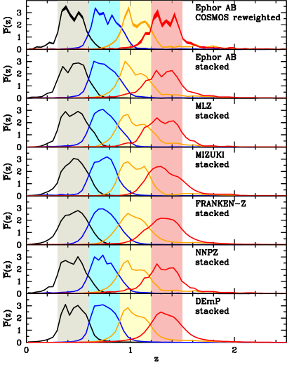
Figure 3: Comparison of COSMOS-reweighted redshift distribution for the four tomographic bins with corresponding redshift distributions obtained by stacking the photo-$z$ PDFs using different photo-$z$ codes; Ephor AB (photo-$z$’s used to define the tomographic bins), MLZ, Mizuki, FRANKEN-Z, NNPZ, and DEmP. Shaded regions show our definition of 4 tomographic bins for best photo-$z$’s, i.e., $0.3<z<0.6$, $0.6<z<0.9$, $0.9<z<1.2$, and $1.2<z<1.5$. The shaded region around each curve in the top panel shows the statistical error of the COSMOS-reweighted redshift distributions estimated by the bootstrap resampling technique. In our cosmology analysis, we take account of these differences of redshift distributions $\bar{P}(z)$ using $z$-shift parameter $\Delta z$ [equation (31)]. We also discuss the impact of different $\bar{P}(z)$ on cosmological parameters in Section 6.2.

Table 3: Summary of the photo-$z$ distribution for each method.

photo-$z$ method	$0.3<z<0.6$	$0.6<z<0.9$	$0.9<z<1.2$	$1.2<z<1.5$
Fiducial	0.44 ( 6.1%), 0.43, 0.11	0.77 ( 3.6%), 0.75, 0.12	1.05 (12.6%), 1.03, 0.13	1.33 ( 5.9%), 1.31, 0.15
Ephor AB	0.45 ( 7.4%), 0.44, 0.12	0.75 ( 5.1%), 0.76, 0.12	1.04 ( 7.2%), 0.98, 0.16	1.32 ( 4.8%), 1.29, 0.19
MLZ	0.46 ( 2.8%), 0.46, 0.12	0.75 ( 2.3%), 0.74, 0.11	1.04 ( 3.2%), 1.02, 0.13	1.32 ( 1.6%), 1.31, 0.16
Mizuki	0.45 ( 3.3%), 0.46, 0.10	0.74 ( 1.8%), 0.74, 0.10	1.04 ( 3.0%), 1.04, 0.10	1.33 ( 1.2%), 1.32, 0.12
Franken-Z	0.45 ( 5.9%), 0.46, 0.12	0.75 ( 3.3%), 0.74, 0.13	1.04 ( 7.3%), 1.03, 0.14	1.34 ( 4.3%), 1.33, 0.16
NNPZ	0.44 ( 6.7%), 0.44, 0.11	0.74 ( 4.0%), 0.73, 0.12	1.03 ( 8.6%), 1.01, 0.12	1.33 ( 7.9%), 1.31, 0.14
DEmP	0.45 ( 5.9%), 0.45, 0.11	0.75 ( 3.6%), 0.74, 0.11	1.04 ( 6.2%), 1.02, 0.13	1.34 ( 6.5%), 1.32, 0.16

^∗We show the mean, median, and $1\sigma$ dispersion of the photo-$z$ distribution for each method, for each of the 4-bin tomographic bins, as shown in Figure 3. The mean value is estimated by clipping the distribution outside the $3\sigma$ range, where the clipping is repeated until the mean value converges. The values in parentheses denote the clipped fractions, which reflect outlier fractions of photo-$z$’s of individual galaxies.

In addition, we take account of the multiplicative selection bias $m_{\rm sel}$ due to cuts in the resolution factor that characterize galaxy size. Mandelbaum et al. (2018b) found that the selection bias is proportional to the fraction of galaxies at the sharp boundary of galaxy size cut (the resolution factor $R_{2}$ in our terminology) as $m_{\rm sel}=A\times p(R_{2}=0.3)$ with $A=0.0087\pm 0.0026$. We use this formula to estimate the selection bias in each tomographic bin. It is found that $m_{\rm sel}$ is at the level of 0.01, as listed in Table 4. Since the statistical errors in $m_{\rm sel}$ are $\sim 0.003$ and therefore are smaller than $\Delta m$ introduced above, we ignore the statistical error of $m_{\rm sel}$.

Furthermore, we also include the responsivity correction due to the dependence of the intrinsic ellipticity variations on redshift. In the HSC first-year shear catalog, the intrinsic ellipticity was estimated as a function of $S/N$ and resolution factor $R_{2}$ using image simulations (Mandelbaum et al., 2018b). Inferring the intrinsic ellipticity dispersion required us to separate out the measurement error contribution to the total shape variance. This separation was carried out using pairs of galaxies simulated at 90^∘ with respect to each other, for which we derived an analytic method of inferring the measurement error contribution to the total shape variance. Once we have estimated the measurement error contribution as a function of galaxy properties, it is possible to infer the intrinsic shape noise dispersion (assuming independence of the measurement error and intrinsic shape contributions for each galaxy). We recently found that the intrinsic ellipticity varies with redshift such that the intrinsic rms error $e_{\rm rms}$ is smaller between $1<z<1.5$ than that at other redshifts. This variation of $e_{\rm rms}$ affects our cosmic shear signals via the responsivity factor. We include this correction in our theoretical model by introducing an additional multiplicative bias factor $m_{\cal R}$, which has the value $m_{\cal R}=0.015$ for $0.9<z<1.2$, $m_{\cal R}=0.03$ for $1.2<z<1.5$, and zero otherwise (see Section 5.3 of Mandelbaum et al., 2018b).

Together with the uncertainty of the original multiplicative bias factor in equation (29), we correct the theoretical model of tomographic lensing power spectra as

$$C_{\ell}^{(ij)}\rightarrow(1+\Delta m)^{2}(1+m_{\rm sel}^{(i)}+m_{\cal R}^{(i)})(1+m_{\rm sel}^{(j)}+m_{\cal R}^{(j)})C_{\ell}^{(ij)},$$ (30)

where $\Delta m$ is a model parameter with Gaussian prior, and $m_{\rm sel}^{(i)}$ and $m_{\cal R}^{(i)}$ are fixed numbers listed in Table 4.

Table 4: Multiplicative bias correction factors associated with the selection bias due to cuts in the resolution factor, $m_{\rm sel}$, and with the responsivity correction due to intrinsic ellipticity variations with redshifts, $m_{\cal R}$, for the four tomographic bins.

$z$ range	$100m_{\rm sel}$	$100m_{\cal R}$
0.3 – 0.6	0.86	0.0
0.6 – 0.9	0.99	0.0
0.9 – 1.2	0.91	1.5
1.2 – 1.5	0.91	3.0

5.8 Redshift distribution uncertainty

In our cosmological analysis, we take into account uncertainty in the redshift distribution of our source galaxies by comparing redshift distributions of source galaxies from the reweighting method to that of the stacked photo-$z$ PDF method, as well as the difference of stacked photo-$z$ PDFs among different photo-$z$ codes. Figure 3 shows the comparison of the COSMOS-reweighted redshift distribution with stacked photo-$z$ PDFs [equation (19)] among different photo-$z$ codes (Tanaka et al., 2018) (also see Section 2) for all four tomographic bins. Statistical uncertainties in the COSMOS-reweighted redshift distributions are estimated by the bootstrap resampling technique.

Table 5: The methodological errors $\Delta z_{i}$ and the code uncertainties $\sigma^{\rm code}_{\Delta z_{i}}$, as well as the total photo-$z$ uncertainties $\sigma_{\Delta z_{i}}^{\rm tot}$ from the quadrature sum of these two uncertainties, for the four tomographic bins.

$z$ range	$100{\Delta z_{i}}^{\rm method}$	$100\sigma_{\Delta z_{i}}^{\rm code}$	$100\sigma_{\Delta z_{i}}^{\rm tot}$
0.3 – 0.6	2.66	1.01	2.85
0.6 – 0.9	$-1.07$	0.83	1.35
0.9 – 1.2	$-3.79$	0.55	3.83
1.2 – 1.5	$-3.20$	1.98	3.76

Model predictions of cosmic shear signals depend crucially on redshift distributions of source galaxies (see Section 5.1), suggesting that it is important to take proper account of photo-$z$ uncertainties and especially the effect of the photo-$z$ errors on the mean of the redshift distribution in each tomographic bin. We quantify the impact of the photo-$z$ error on the cosmic shear power spectrum using the $z$-shift parameter $\Delta z_{i}$, which uniformly shifts the redshift distribution of source galaxies in the $i$-th tomographic bin as

$$\bar{P}^{(i)}(z)\rightarrow\bar{P}^{(i)}(z+\Delta z_{i}).$$ (31)

For each estimate of the redshift distribution that is different from the fiducial one, we derive a value of $\Delta z_{i}$ so that the cosmic shear power spectrum amplitude computed using that $\bar{P}^{(i)}(z)$ matches our fiducial cosmic shear power spectrum computed using the COSMOS-reweighted $\bar{P}^{(i)}(z)$. We have verified that given the signal-to-noise ratio of our cosmic shear measurements, the shifts that we consider here cannot be distinguished from differences in the shape of the redshift distribution.

We estimate photo-$z$ uncertainties in two different ways in order to avoid any double counting of photo-$z$ uncertainties. First, we evaluate $\Delta z_{i}$ between the fiducial COSMOS-reweighted $\bar{P}^{(i)}(z)$ and those obtained by using the stacked photo-$z$ PDFs using the Ephor AB code. This $\Delta z_{i}$, which we denote $\Delta z_{i}^{\rm method}$, represents the methodological uncertainty. Next, we evaluate the photo-$z$ uncertainties due to the photo-$z$ algorithm as the scatter of $\Delta z_{i}$ among the six photo-$z$ codes (see Figure 3). Specifically, for each photo-$z$ code we estimate $\Delta z_{i}$ between the fiducial COSMOS-reweighted $\bar{P}^{(i)}(z)$ and the stacked photo-$z$ PDF from that photo-$z$ code by matching the amplitudes of the cosmic shear power spectrum, and regard the standard deviation, $\sigma^{\rm code}_{\Delta z_{i}}$, among the six $\Delta z_{i}$ from the six photo-$z$ codes as the photo-$z$ uncertainty due to the photo-$z$ algorithm. We present more details of these photo-$z$ distributions Table 3, in which we list the mean, median, and 1$\sigma$ dispersion of each distribution.

We list values of $\Delta z_{i}^{\rm method}$ and $\sigma_{\Delta z_{i}}^{\rm code}$ for the four tomographic bins in Table 5. We find that $\left|\Delta z_{i}^{\rm method}\right|$ is at the level of $0.03-0.04$ except for the lower-intermediate redshift bin. In contrast, $\sigma_{\Delta z_{i}}^{\rm code}$ is $\lesssim 0.02$ and therefore is smaller than $\Delta z_{i}^{\rm method}$. In our cosmic shear analysis, we combine these two uncertainties in quadrature

$$\sigma_{\Delta z_{i}}^{\rm tot}=\sqrt{(\Delta z_{i}^{\rm method})^{2}+(\sigma_{\Delta z_{i}}^{\rm code})^{2}},$$ (32)

and for each tomographic bin we include $\Delta z_{i}$ as defined in equation (31) as a model parameter with Gaussian prior, and set the mean and standard deviation of the Gaussian prior to zero and $\sigma_{\Delta z_{i}}^{\rm tot}$, respectively. The values of $\sigma_{\Delta z_{i}}^{\rm tot}$ for the four tomographic bins are listed in Table 5. We find that the statistical errors of the COSMOS-reweighted redshift distributions estimated by bootstrap resampling translate into values $\Delta z_{i}$ that are a factor of 5-10 times smaller than $\sigma_{\Delta z_{i}}^{\rm tot}$. Thus this source of statistical errors is negligible, and we do not explicitly account for it.

The procedure above assumes that uncertainties of photo-$z$’s in individual bins are parametrized by single parameters $\Delta z_{i}$, which might be too simplistic. To check the robustness of our results to changes in redshift distributions such as outlier fractions, in Section 6.2.2 we will conduct a robustness check in which we replace $\bar{P}(z)$ from the fiducial COSMOS reweighted method with those from stacked photo-$z$ PDFs with different photo-$z$ codes.

Table 6: Summary of parameters and priors used in our nested sampling analysis of tomographic cosmic shear power spectra.^∗

Parameter	symbols	prior
physical dark matter density	$\Omega_{\rm c}h^{2}$	flat [0.03,0.7]
physical baryon density	$\Omega_{\rm b}h^{2}$	flat [0.019,0.026]
Hubble parameter	$h$	flat [0.6,0.9]
scalar amplitude on $k=0.05$Mpc-1	$\ln(10^{10}A_{s})$	flat [1.5,6]
scalar spectral index	$n_{\rm s}$	flat [0.87,1.07]
optical depth	$\tau$	flat [0.01,0.2]
neutrino mass	$\sum m_{\nu}$ [eV]	fixed (0)†, fixed (0.06) or flat [0,1]
dark energy EoS parameter	$w$	fixed ($-1$)† or flat $[-2,-0.333]$
amplitude of the intrinsic alignment	$A_{\rm IA}$	flat $[-5,5]$
redshift dependence of the intrinsic alignment	$\eta_{\rm eff}$	flat $[-5,5]$
baryonic feedback amplitude	$A_{B}$	fixed (0)† or flat $[-5,5]$
PSF leakage	$\tilde{\alpha}$	Gauss $(0.057,0.018)$
residual PSF model error	$\tilde{\beta}$	Gauss $(-1.22,0.74)$
uncertainty of multiplicative bias $m$	$100\Delta m$	Gauss $(0,1)$
photo-$z$ shift in bin 1	$100\Delta z_{1}$	Gauss $(0,2.85)$
photo-$z$ shift in bin 2	$100\Delta z_{2}$	Gauss $(0,1.35)$
photo-$z$ shift in bin 3	$100\Delta z_{3}$	Gauss $(0,3.83)$
photo-$z$ shift in bin 4	$100\Delta z_{4}$	Gauss $(0,3.76)$

^∗In our fiducial analysis, we vary five cosmological parameters ($\Omega_{\rm c}h^{2}$, $\Omega_{\rm b}^{2}$, $h$, $A_{s}$, and $n_{s}$) within the $\Lambda$CDM model and an additional parameter $w$ in the $w$CDM model, two parameters to model the IA (amplitude $A_{\rm IA}$ and the power-law index of the redshift dependence $\eta_{\rm eff}$), and seven additional nuisance parameters; PSF leakage $\tilde{\alpha}$, residual PSF model error $\tilde{\beta}$, the multiplicative bias error $\Delta m$, and photo-$z$ mean shift values $\Delta z_{i}$ for the four tomographic bins. Optical depth $\tau$ is not used when analyzing cosmic shear measurements only, but is included when CMB datasets are combined, and its prior is indicated in italics. There are three types of priors; fixed ($x$) means the value is fixed to be $x$; flat $[x,y]$ means a flat prior between $x$ and $y$, and Gauss $(x,y)$ means a Gaussian prior with mean value $x$ and standard deviation $y$. In our fiducial analysis, the neutrino mass $\sum m_{\nu}$ is fixed to be 0 and the baryonic feedback amplitude $A_{B}$ is fixed to be 0 when the baryonic effect is not included [see equation (28)]. The parameter $A_{B}$ is included as a model parameter only when we check the robustness of our results in Section 6.2. When we have multiple priors for each parameter, priors with ^† indicate those adopted in our fiducial $\Lambda$CDM model analysis.

5.9 Posterior distribution of parameters using nested sampling

We draw samples from the posterior distribution of parameters given the cosmic shear signal with the help of nested sampling as implemented in the publicly available Multinest (Multi-Modal Nested Sampler) code (Feroz & Hobson, 2008; Feroz et al., 2009, 2013; Buchner et al., 2014) together with the package Monte Python (Audren et al., 2013). The log-likelihood of the data given our parameters obeys the following equation,

$$-2\ln\mathcal{L} = \sum_{iji^{\prime}j^{\prime}}\sum_{b,b^{\prime}}^{\ell_{\rm min}\leq\ell_{b},\ell_{b^{\prime}}\leq\ell_{\rm max}}\Delta C_{b}^{(ij)}\left[{\rm Cov}\right]^{-1}\Delta C_{b^{\prime}}^{(i^{\prime}j^{\prime})}$$ (33)

$$+\ln|{\rm Cov}|+{\rm const},$$

where $\Delta C_{b}^{(ij)}$ is the difference between measured (Section 4) and model (Section 5) cosmic shear power spectra, and $i$ and $j$ refer to different tomographic bins. The latter is a function of cosmological parameters as well as various nuisance parameters. Given that we measure the cosmic shear power spectra in multipole bins [see equation (8)], the model predictions must be computed as a bin-average of the theoretical power spectra weighted by the number of modes present at each multipole within the bin. To be explicit, we compute the model power spectrum in each multipole bin, $C^{\rm model}_{b}$, as

$$C^{\rm model}_{b}=\frac{\sum_{\bm{\ell}}^{\ell\in\ell_{b}}P_{b\ell}C_{\ell}^{\rm model}}{\sum_{\bm{\ell}}^{\ell\in\ell_{b}}P_{b\ell}},$$ (34)

where $\ell=|{\bm{\ell}}|$, $P_{b\ell}=\ell^{2}/2\pi$ is the conversion factor to the dimensionless power spectrum. When computing $C^{\rm model}_{b}$, the summation over ${\bm{\ell}}$ in each multipole bin is matched to the measured spectra as in equation (8) The covariance matrix is estimated by an analytic model and also depends on cosmological parameters (see Section 5.3). Since we adopt a cosmology-dependent covariance matrix, we include the determinant of the covariance, $|{\rm Cov}|$, in the expression of our log-likelihood.

The cosmological parameter set we use is summarized in Table 6. We include the standard $\Lambda$CDM cosmological parameters, such as the dark matter density $\Omega_{\rm c}h^{2}$, the baryon density $\Omega_{\rm b}h^{2}$, the dimensionless Hubble constant $h$, the scalar spectral index $n_{\rm s}$, the amplitude of the primordial curvature perturbation $A_{s}$ with reasonably broad flat priors. In the fiducial case, the neutrino mass is fixed to be zero. As we will show later, our results do not change significantly when we apply the lower bound of the absolute sum of neutrino mass, $\sim 0.06$ eV, indicated from the neutrino oscillation experiments (e.g., see Lesgourgues et al., 2013, for a review). We also constrain models where the dark energy equation of state parameter $w$ is allowed to vary, in our extended analysis. When combining with CMB datasets, we add the free-electron scattering optical depth $\tau$ as an additional parameter. In addition to these cosmological parameters, we constrain two parameters for IA, the amplitude $A_{\rm IA}$ and the redshift-dependence power-law index $\eta_{\rm eff}$, as well as seven additional nuisance parameters to model uncertainties in shear and photo-$z$ measurements.

We check the convergence of nested sampling using nestcheck (Higson, 2018), which is a publicly available code to assess the convergence of the posterior distribution and implementation-specific error due to the correlated samples and missing parts of the posterior. We find that each run terminates when the remaining posterior mass is sufficiently small. We also find no significant implementation-specific errors. Details of this convergence test are given in Appendix C. As a sanity check, we also derive the posterior distributions using the traditional Markov-Chain Monte-Carlo algorithm implemented in the CosmoMC code (Lewis & Bridle, 2002) and find excellent agreement with the posterior distribution of our parameters obtained from nested sampling.

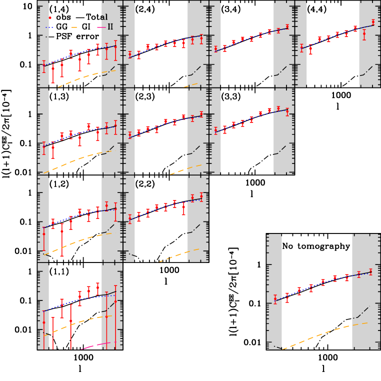
Figure 4: Comparison of the measured tomographic shear power spectra with our theoretical model with best-fit values for the fiducial $\Lambda$CDM model. Best-fit IA power spectra of $C_{\rm GG}$ (dotted), $-C_{\rm GI}$ (short dashed), and $C_{\rm II}$ (long dashed) as well as power spectra arising from PSF leakage and PSF model error [equation (13)] (dash-dotted) are also plotted. The redshift range of $z_{\rm best}$ in each tomographic bin is =$[0.3,0.6]$, $[0.6,0.9]$, $[0.9,1.2]$, and $[1.2,1.5]$ from 1 to 4. The right-bottom panel shows the measured non-tomographic cosmic shear power spectrum and the model spectra with the best-fit values from the tomographic analysis. The $C_{\rm II}$ term is so small that it is absent from all panels except for 11.

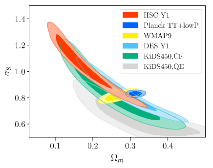
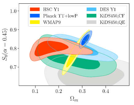
Figure 5: Marginalized posterior contours in the $\Omega_{\rm m}$-$\sigma_{8}$ plane (left) and in the $\Omega_{\rm m}$-$S_{8}(\alpha=0.45)$ plane (right), where $S_{8}(\alpha)\equiv\sigma_{8}(\Omega_{\rm m}/0.3)^{\alpha}$, in the fiducial $\Lambda$CDM model. Both 68% and 95% credible levels are shown. For comparison, we plot cosmic shear results from KiDS-450 with correlation function (CF) estimators (Hildebrandt et al., 2017) and with quadratic estimators (QE) (Köhlinger et al., 2017) and DES Y1 (Troxel et al., 2018b) with the same set of cosmological parameters and priors as adopted in this paper, as well as WMAP9 (Hinshaw et al., 2013) (yellow) and Planck 2015 CMB constraints without CMB lensing (Planck Collaboration et al., 2016) (purple).

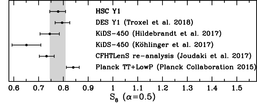
Figure 6: The 68% credible interval on $S_{8}(\alpha=0.5)$ from the HSC first-year data in the $\Lambda$CDM model as well as from several literature.

6 Cosmological constraints from tomographic cosmic shear power spectra

In this section, we present cosmological constraints from tomographic cosmic shear power spectra measured with the HSC first-year data in the $\Lambda$CDM model. We also test the robustness of our cosmological constraints against various systematics including shape measurement errors, photo-$z$ uncertainties, intrinsic alignment modeling, baryon physics, and uncertainty in neutrino mass. We next perform internal consistency checks by adopting different ranges of $\ell$ and $z$ bins. We then extend our fiducial analysis to $w$CDM, as well as combine our results with the Planck CMB result to check the consistency of the results and to constrain cosmological parameters including neutrino mass, intrinsic alignment and the baryon feedback parameter.

6.1 Cosmological constraints in the $\Lambda$CDM model

First, we compare the measured cosmic shear power spectra with our best-fitting model in Figure 4. We compute $\chi^{2}$ of our best-fitting model as

$$\chi^{2} = \chi^{2}_{\rm data}+\chi^{2}_{\rm Gauss},$$ (35)

$$\chi^{2}_{\rm data} = \sum_{bb^{\prime}}({\cal C}_{b}^{\rm obs}-{\cal C}_{b}^{\rm model})[{\rm Cov}]^{-1}({\cal C}_{b^{\prime}}^{\rm obs}-{\cal C}_{b^{\prime}}^{\rm model}),$$ (36)

$$\chi^{2}_{\rm Gauss} = \sum_{j}[(p_{j}^{\rm obs}-\bar{p}_{j})/\sigma_{j}]^{2}.$$ (37)

where $\chi^{2}_{\rm data}$ comes from the tomographic E-mode spectra and $\chi^{2}_{\rm Gauss}$ comes from parameters with Gaussian priors, i.e., $\tilde{\alpha}$, $\tilde{\beta}$, $\Delta m$, and $\Delta z_{i}$ ($i=1-4$), and $\bar{p}_{j}$ and $\sigma_{j}$ indicate the mean value and the standard deviation of each prior, respectively (see Table 6). The degree-of-freedom (DOF) is computed as

$${\rm DOF}=N_{\rm data}-N_{\rm eff},$$ (38)

where $N_{\rm data}$ is 60, corresponding to the number of data points of the tomographic E-mode spectra in the 4 tomographic bins (Figure 4), and $N_{\rm eff}$ represents the effective number of parameters that the data constrain. We compute $N_{\rm eff}$ as (Raveri & Hu, 2018)

$$N_{\rm eff}=N_{\rm para}-{\rm tr}[{\cal C}_{\rm prior}^{-1}{\cal C}_{\rm post}],$$ (39)

where $N_{\rm para}$ is the number of parameters including both cosmology and nuisance parameters (14 in the fiducial setup), ${\cal C}_{\rm prior}$ is the covariance of prior distributions, and ${\cal C}_{\rm post}$ is the covariance of posterior distributions. The effective number of parameters account for parameters that are dominated by the parameters whose posteriors are driven by data rather than the priors. We find that $N_{\rm eff}$ is 3.1, which results in DOF of 56.9. The difference between $N_{\rm eff}$ and the total number of parameters in our model reflects the fact that a number of our model parameters are prior-dominated.

We find that our model well reproduces the observed power spectra quite well. Our maximum-likelihood case in the fiducial $\Lambda$CDM model has a minimum $\chi^{2}$ of 45.4 for 56.9 DOF ($p$-value is 0.86), which is a very acceptable fit. Using the covariance assuming Planck cosmology, the total signal-to-noise ratio, estimated as $[\sum_{bb^{\prime}}{\cal C}_{b}^{\rm obs}[{\rm Cov}]^{-1}{\cal C}_{b^{\prime}}^{\rm obs}]^{1/2}$, in the four bin tomographic lensing spectra is $15.6$ in the fiducial range of multipoles. The signal-to-noise ratios of the cosmic shear auto spectra in individual redshift bins are 4.9, 9.2, 12.3, and 11.5 from the lowest to the highest redshift bins, respectively. Although the number of source galaxies in the higher redshift bins is less than in the lower redshift bins, the signal-to-noise ratios of the measurements are higher due to the higher amplitudes of the cosmic shear power spectra.

We derive marginalized posterior contours in the $\Omega_{\rm m}$-$\sigma_{8}$ plane from our tomographic cosmic shear power spectrum analysis in the fiducial $\Lambda$CDM model. Constraints from cosmic shear are known to be degenerate in the $\Omega_{\rm m}$-$\sigma_{8}$ plane. Cosmic shear can tightly constrain a combination of cosmological parameters $S_{8}(\alpha)\equiv\sigma_{8}(\Omega_{\rm m}/0.3)^{\alpha}$, which we adopt to quantify cosmological constraints from the HSC first year data. By carrying out a linear fit of the logarithm of the posterior samples of $\Omega_{\rm m}$ and $\sigma_{8}$, we find that the tightest constraints for $S_{8}$ are obtained with $\alpha=0.45$. However, the previous studies by DES (Troxel et al., 2018a) and KiDS (Hildebrandt et al., 2017; Köhlinger et al., 2017) have presented constraints on $S_{8}$ with $\alpha=0.5$. To present best constraints as well as constraints that can be directly compared with these previous cosmic shear results, in this paper we present our results of $S_{8}$ both for $\alpha=0.45$ and $\alpha=0.5$.

In Figure 5, we show our marginalized constraints in $\Omega_{\rm m}$-$\sigma_{8}$ and $\Omega_{\rm m}$-$S_{8}(\alpha=0.45)$ planes. As expected, there is no strong correlation between $\Omega_{\rm m}$ and $S_{8}$. We find $S_{8}(\alpha=0.45)=0.800^{+0.029}_{-0.028}$ and $\Omega_{\rm m}=0.162^{+0.086}_{-0.044}$. Our HSC first-year cosmic shear analysis places a 3.6% fractional constraint on $S_{8}$, which is comparable to the results of DES (Troxel et al., 2018a) and KiDS (Hildebrandt et al., 2017). For comparison, we find a slightly degraded constraint on $S_{8}(\alpha=0.5)=0.780^{+0.030}_{-0.033}$ for $\alpha=0.5$. We compare our constraints in the $\Omega_{\rm m}$-$\sigma_{8}$ and $\Omega_{\rm m}$-$S_{8}(\alpha=0.5)$ planes with cosmic shear results from DES Y1 (Troxel et al., 2018b) and also from KiDS-450 with two different methods, correlation functions (CF; Hildebrandt et al., 2017) and quadratic estimators (QE; Köhlinger et al., 2017). Note that the plotted results from DES Y1 use the same set of cosmological parameters and priors as adopted in this paper, and are different from the fiducial constraints in Troxel et al. (2018b). For the KiDS results, we show the same constraints as shown in the literature but not corrected for the noise covariance (Troxel et al., 2018b). We also note that there are also some differences in the choice of parameters and priors. KiDS adopt wider priors on $\Omega_{c}h^{2}$ and $n_{s}$, while $h$ prior is narrower and non-flat (instead KiDS adopt a flat prior on the approximated sound horizon scale $\theta_{\rm MC}$). The impact of the difference between $\theta_{\rm MC}$ and $h$ is found to be small (Hildebrandt et al., 2017; Troxel et al., 2018b). The choice of priors and their ranges can impact especially on the degeneracy direction between $\Omega_{m}$ and $\sigma_{8}$ (e.g., Chang et al., 2019). Figure 6 compares the values of $S_{8}(\alpha=0.5)$ and their 1-$\sigma$ errors among recent cosmic shear studies. We find that there is no significant difference between the $S_{8}$ values obtained by these independent studies. Our result for $S_{8}$ is smaller than the DES results by 0.5$\sigma$ and larger than the KiDS results by 1$\sigma$ or 2$\sigma$ for the CF and QE estimators. The difference becomes smaller when the shape noise covariance is corrected in the KiDS results (Troxel et al., 2018b).

Our best-fit $\Omega_{\rm m}$ value is smaller than that obtained by other lensing surveys. More specifically, the best-fit $\Omega_{\rm m}$ values from DES and KiDS are 1.3$\sigma$ and 1$\sigma$ larger than our best-fit value, respectively. We also compare these cosmic shear constraints with Planck CMB constraints (Planck Collaboration et al., 2016). We find that Planck best-fit values of $S_{8}$ and $\Omega_{\rm m}$ are 2$\sigma$ and 1.8$\sigma$ higher than our best-fit values, where we take into account of the uncertainties in both measurements. We check the consistency between our result and Planck CDM constraints more quantitatively in Section 6.3. Our result prefers slightly lower $S_{8}$ and $\Omega_{\rm m}$ values than the Planck CMB results, which is qualitatively consistent with other cosmic shear results from DES and KiDS, as discussed in the recent Planck 2018 paper (Planck Collaboration et al., 2018).

As discussed above, our result shows a small best-fit value of $\Omega_{\rm m}$, as well as a relatively tight constraint on $\Omega_{\rm m}$. While tomographic analysis has been shown to improve measurements of $\Omega_{\rm m}$ and $\sigma_{8}$ (e.g., Simon et al., 2004), we check whether the small errorbar is expected given our sample size and tomographic bin definition. For this purpose, we again use the HSC mock shear catalogs, which were also used to check the validity and accuracy of the pseudo-$C_{\ell}$ method (see Section 3.1). We perform nested sampling analysis on the 100 mock catalogs adopting the same set of cosmological and nuisance parameters as in the analysis of the real HSC data, and for each mock we derive both the best-fit value and 1$\sigma$ error of $\Omega_{\rm m}$. We find that the best-fit value and the 1$\sigma$ error of $\Omega_{\rm m}$ are positively correlated. Our result indicates that 4 out of 100 mock realizations have both smaller best-fit values and tighter constraints on $\Omega_{\rm m}$ than the observed values. Although this mock catalog analysis is based on a specific cosmological model (WMAP9), it suggests that the observed small best-fit value and the tight constraint on $\Omega_{\rm m}$ can be explained by a statistical fluctuation at the 2$\sigma$ level, and therefore they do not necessarily indicate the presence of systematic errors (see also Section 6.2).

Table 7: Summary of the median and 68% range of uncertainties of $S_{8}(\alpha)$ with $\alpha=0.45$ and $0.5$ and $\Omega_{\rm m}$, as well as their robustness against various systematics, in the $\Lambda$CDM model from our cosmic shear measurements.^∗ Constraints assuming the $w$CDM cosmology are also shown in the bottom row of the table.

setup	$S_{8}(\alpha=0.45)$	$S_{8}(\alpha=0.5)$	$\Omega_{\rm m}$
Fiducial	$0.800_{-0.028}^{+0.029}$	$0.780_{-0.033}^{+0.030}$	$0.162_{-0.044}^{+0.086}$
w/o shape error ($\tilde{\alpha}=\tilde{\beta}=\Delta m=0$)	$0.801_{-0.028}^{+0.028}$	$0.783_{-0.030}^{+0.028}$	$0.177_{-0.055}^{+0.098}$
w/o photo-$z$ error ($\Delta z_{i}=0$)	$0.804_{-0.028}^{+0.027}$	$0.784_{-0.033}^{+0.029}$	$0.162_{-0.046}^{+0.085}$
Ephor AB, stacked	$0.818_{-0.029}^{+0.029}$	$0.799_{-0.032}^{+0.029}$	$0.172_{-0.049}^{+0.083}$
MLZ, stacked	$0.813_{-0.028}^{+0.028}$	$0.801_{-0.028}^{+0.027}$	$0.221_{-0.073}^{+0.098}$
Mizuki, stacked	$0.807_{-0.027}^{+0.027}$	$0.791_{-0.027}^{+0.027}$	$0.195_{-0.055}^{+0.085}$
NNPZ, stacked	$0.818_{-0.029}^{+0.029}$	$0.807_{-0.027}^{+0.027}$	$0.231_{-0.076}^{+0.112}$
Frankenz, stacked	$0.809_{-0.030}^{+0.030}$	$0.789_{-0.037}^{+0.032}$	$0.164_{-0.048}^{+0.090}$
DEmP, stacked	$0.812_{-0.029}^{+0.028}$	$0.791_{-0.034}^{+0.029}$	$0.163_{-0.044}^{+0.076}$
w/o IA ($A_{\rm IA}=0$)	$0.787_{-0.028}^{+0.027}$	$0.767_{-0.031}^{+0.028}$	$0.172_{-0.051}^{+0.079}$
$\eta_{\rm eff}$ fixed to be $3$	$0.800_{-0.032}^{+0.031}$	$0.776_{-0.038}^{+0.034}$	$0.152_{-0.041}^{+0.062}$
$\sum m_{\nu}$ fixed to be 0.06 eV	$0.797_{-0.029}^{+0.029}$	$0.777_{-0.034}^{+0.031}$	$0.166_{-0.047}^{+0.088}$
$\sum m_{\nu}$ varied	$0.785_{-0.031}^{+0.029}$	$0.765_{-0.038}^{+0.031}$	$0.175_{-0.049}^{+0.090}$
$A_{B}$ varied	$0.797_{-0.041}^{+0.039}$	$0.775_{-0.048}^{+0.047}$	$0.157_{-0.048}^{+0.092}$
AGN feedback model ($A_{\rm B}=1$)	$0.818_{-0.029}^{+0.029}$	$0.804_{-0.031}^{+0.030}$	$0.201_{-0.064}^{+0.104}$
w/o lowest $z$-bin	$0.799_{-0.032}^{+0.032}$	$0.779_{-0.034}^{+0.033}$	$0.165_{-0.049}^{+0.097}$
w/o mid-low $z$-bin	$0.799_{-0.030}^{+0.030}$	$0.795_{-0.028}^{+0.028}$	$0.283_{-0.109}^{+0.109}$
w/o mid-high $z$-bin	$0.791_{-0.035}^{+0.033}$	$0.770_{-0.037}^{+0.034}$	$0.156_{-0.046}^{+0.107}$
w/o highest $z$-bin	$0.797_{-0.034}^{+0.034}$	$0.780_{-0.033}^{+0.033}$	$0.186_{-0.058}^{+0.099}$
$\ell_{\rm max}$ extended to 3500	$0.801_{-0.026}^{+0.027}$	$0.780_{-0.030}^{+0.028}$	$0.166_{-0.042}^{+0.060}$
Lower half $\ell$-bin	$0.799_{-0.038}^{+0.038}$	$0.783_{-0.039}^{+0.037}$	$0.182_{-0.065}^{+0.138}$
Higher half $\ell$-bin	$0.799_{-0.031}^{+0.033}$	$0.789_{-0.029}^{+0.030}$	$0.235_{-0.079}^{+0.107}$
fixed covariance with best-fit cosmology	$0.806_{-0.031}^{+0.030}$	$0.785_{-0.033}^{+0.032}$	$0.173_{-0.049}^{+0.088}$
$w$CDM	$0.773_{-0.038}^{+0.043}$	$0.754_{-0.049}^{+0.044}$	$0.163_{-0.047}^{+0.079}$

^∗The values of $S_{8}(\alpha=0.45)$ are also illustrated in Figure 7.

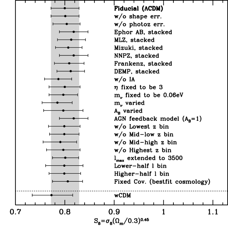
Figure 7: Constraints on $S_{8}(\alpha)\equiv\sigma_{8}(\Omega_{\rm m}/0.3)^{\alpha}$ with $\alpha=0.45$ and their robustness against various systematics and modeling choices in the $\Lambda$CDM model. The shaded area shows the 68% credible interval for the $S_{8}$ value for $\alpha=0.45$ in our fiducial case. We consider the effects of shape and photo-$z$ uncertainties, impacts of assumptions on IA modeling, baryonic feedback modeling, varying neutrino mass, and different ranges of $\ell$ and $z$ bins (see Section 6.2 for more details). Constraints based on the $w$CDM model are also shown at the bottom. We find that the systematic differences in the $S_{8}$ values are well within the 1$\sigma$ statistical error, indicating that our fiducial constraint on $S_{8}$ is robust against these systematics.

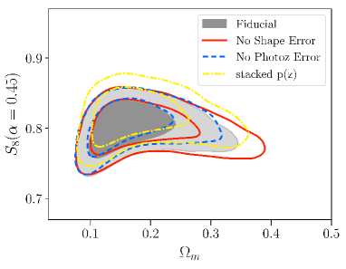
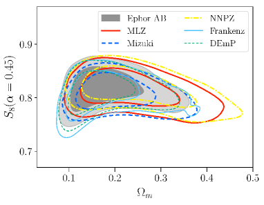
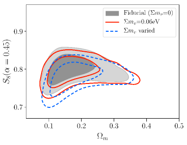
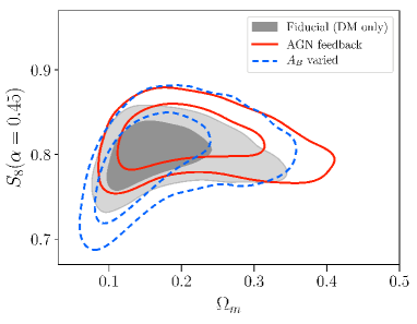
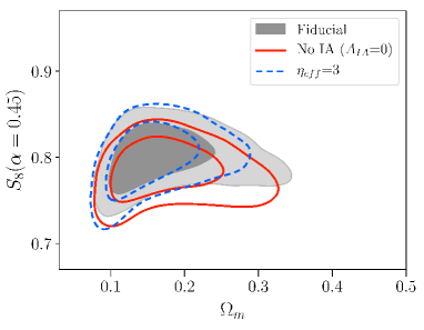
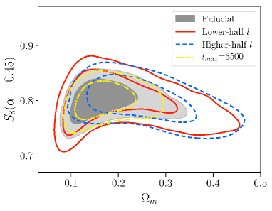
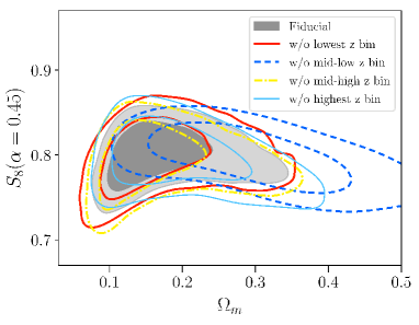
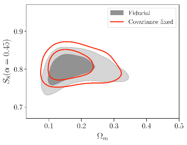
Figure 8: The robustness against various systematics in the $\Omega_{\rm m}$-$S_{8}(\alpha=0.45)$ plane in the fiducial $\Lambda$CDM model. The contours represent 68% and 95% credible levels. Different panels show the robustness against different systematics and modeling choices (see also Table 7 and Figure 7).

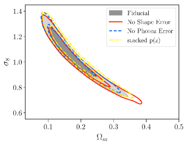
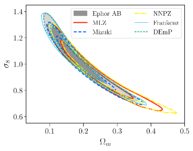
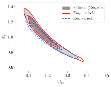
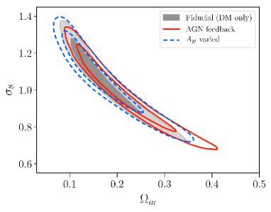
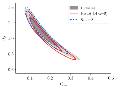
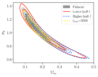
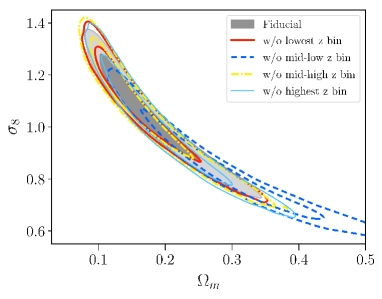
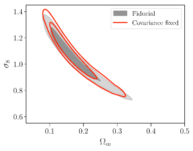
Figure 9: Same as Figure 8 but in the $\Omega_{\rm m}$-$\sigma_{8}$ plane.

6.2 Robustness of our results

To check the robustness of our results, we change the setup of our nested sampling analysis in various ways to see the impact on our cosmological constraints. This includes tests of various systematic effects such as shear measurement errors, photo-$z$ errors, possible contamination by IA, a possible modification in modeling of IA, changes in the matter power spectrum due to baryonic physics and non-zero neutrino mass, as well as internal consistency checks of our results by changing the ranges of $\ell$ and $z$ bins over which the fits are made.

Table 7 and Figure 7 summarize the results of the robustness check in the $\Lambda$CDM model. We list marginalized constraints on $\Omega_{\rm m}$ and $S_{8}(\alpha)\equiv\sigma_{8}(\Omega_{\rm m}/0.3)^{\alpha}$ with $\alpha=0.5$ and 0.45 for each of the tests. In Figures 8 and 9, we show marginalized constraints in the $\Omega_{\rm m}$-$S_{8}$ plane and $\Omega_{\rm m}$-$\sigma_{8}$ for each setup. We also show one-dimensional and two-dimensional posteriors of other cosmological parameters and IA parameters in Appendix D. Below we describe each of the different setups used for the robustness check in detail.

6.2.1 Shape measurement errors

In our fiducial analysis, we account for errors due to the PSF leakage and residual PSF model errors (Section 5.6) and the uncertainty of the multiplicative bias (Section 5.7) by including nuisance parameters to model these errors in the fiducial nested sampling analysis. To check how uncertainties in these treatments propagate into our cosmological constraints, we repeat the nested sampling analysis ignoring these errors (i.e., setting $\tilde{\alpha}=\tilde{\beta}=\Delta m=0$). We find no significant shift in the best-fit values of $S_{8}$ and $\Omega_{\rm m}$ as shown in Table 7 and the top-left panel of Figure 8 for the $\Lambda$CDM model. The shifts of both $S_{8}$ and $\Omega_{\rm m}$ are less than 10% of the statistical error. This indicates that the impact of these shape measurement errors on the current cosmic shear measurement is negligible.

6.2.2 Photometric redshift uncertainties

As discussed in Section 5.8, we include the photo-$z$ uncertainty in the fiducial nested sampling analysis using the additive shift parameter $\Delta z_{i}$. As a simple check, we first ignore these photo-$z$ errors ($\Delta z_{i}=0$) and repeat the nested sampling analysis to find no significant shift or degradation of our $S_{8}$ constraints (see e.g., Figure 8). The result indicates that the photo-$z$ uncertainty does not have a significant impact on the $S_{8}$ constraint compared with the statistical uncertainty of HSC first year data.

However, as was mentioned in Section 5.8, our approach to include photo-$z$ uncertainties by single parameters $\Delta z_{i}$ for individual tomographic bins might be too simplistic. For instance, it might be possible that the true redshift distribution has a small additive shift $\Delta z_{i}$ as compared with our fiducial model, but has a significantly larger outlier fraction. In order to check for possible additional systematics coming from the uncertainty of the redshift distribution that is not captured by the $\Delta z_{i}$ parametrization, we replace the redshift distributions of individual tomographic bins derived from the fiducial COSMOS-reweighted method with stacked photo-$z$ PDFs from the different photo-$z$ codes mentioned in Section 2, and repeat the nested sampling analysis. In doing so we set $\Delta z_{i}=0$. Since the shapes of the redshift distributions are slightly different among different estimates of $\bar{P}(z)$ (see Figure 3), we expect that this test allows us to check the impact of the uncertainty of photo-$z$’s beyond the $\Delta z_{i}$ parameter.

Our results shown in Table 7 indicate that the changes of the median $S_{8}$ values are smaller than the statistical errors, within 0.5$\sigma$ for $\alpha=0.45$. Constraints in the $\Omega_{\rm m}$-$S_{8}$ plane shown in the top-right panel of Figure 8 also indicate that the effect of adopting different photo-$z$ codes is minor, although we can see some shifts in the large $\Omega_{\rm m}$ tails of contours along the $S_{8}$ direction, for some photo-$z$ codes (see Figure 9). Larger effects on the best-fit values of $\Omega_{\rm m}$ can also be seen in e.g., Table 7, however they are accompanied with a corresponding increase in error as well. This is presumably because the minor change of the setup can shift the best-fit values along the degeneracy direction in the $\Omega_{\rm m}$-$\sigma_{8}$ plane, leading to small changes in the $S_{8}$ value itself, but larger changes in the tails of the $S_{8}$ contours along the degeneracy direction that correspond to larger values of $\Omega_{\rm m}$.

6.2.3 Non-zero neutrino mass

In our fiducial setup we assume neutrinos to be massless, i.e., $\sum m_{\nu}$ is set to zero. This is mainly because the inclusion of the minimum value of $\sum m_{\nu}$ of 0.06 eV is expected to have little effect on the matter power spectrum, at least as compared with the statistical error of the HSC first-year cosmic shear analysis. More generally speaking, the HSC cosmic shear or any other large-scale structure probe can constrain mainly $\sigma_{8}$, the present-day matter fluctuation amplitude. The effect of non-zero neutrino mass on large-scale structure observables is absorbed by a change in $\sigma_{8}$. Only when combining the HSC cosmic shear result with CMB constraints can we probe neutrino mass, because a non-zero neutrino mass leads to a suppression in the matter power spectrum amplitude at small scales over the range of low redshifts that the HSC cosmic shear probes, compared to the CMB-inferred $\sigma_{8}$. To check this point explicitly, we include a non-zero neutrino mass of 0.06 eV and repeat the nested sampling analysis, and find that the median value of $S_{8}$ is almost unchanged (see e.g., Figure 8).

We also consider the case in which neutrino mass is allowed to freely vary. While there is a 10% degradation in the 1$\sigma$ error of the $S_{8}$ constraint, the best-fit value is shifted lower by 0.5$\sigma$ (see e.g., second left panel of Figure 8). This can be explained as follows. Non-zero neutrino mass leads to a suppression in the matter power spectrum at scales smaller than the neutrino free-streaming scale relative to large scales within the CDM framework (Takada et al., 2006). Hence, for a fixed $\sigma_{8}$ that we use to normalize the linear matter power spectrum at the present, a model with non-zero neutrino mass leads to greater amplitudes in the matter power spectrum at large scales (low $k$) as well as at higher redshifts, compared to those of the massless neutrino model, i.e. our fiducial model. Hence varying neutrino mass in the parameter inference prefers a slightly smaller value in the best-fit $S_{8}$ in order to reconcile the model with the measured amplitudes of HSC cosmic shear power spectra that are sensitive to the matter power spectrum amplitudes at higher redshifts such as $z\lower 2.15277pt\hbox{$\;\buildrel>\over{\sim}\;$}1$. For the same reason, the best-fit value of $\Omega_{\rm m}$ slightly increases at $\sim 0.2\sigma$ level. However, we note that varying neutrino mass is a physical extension to the fiducial model rather than a systematic effect. When taking into account the recent upper limits on the neutrino mass $<0.12$ eV (95% confidence limit) from Planck 2018 + BAO (Planck Collaboration et al., 2018), the actual shift of the best-fit due to the neutrino mass should be smaller than that estimated above. We will discuss constraints on the neutrino mass from the HSC cosmic shear, Planck, and their combination in Section 6.4.

6.2.4 Baryonic feedback effect

As described in Section 5.5, we do not include the modification of the matter power spectrum due to baryonic physics in our fiducial setup, but we explore the impact of baryonic physics in the robustness check. As a first check, we fix the matter power spectrum to that in the AGN feedback model ($A_{B}=1$), and find that the $S_{8}$ value is indeed shifted to a larger value to compensate for the small-scale suppression of the lensing power. The shift of the best-fit $S_{8}$ value is at most $\sim 0.6\sigma$ even in this extreme AGN feedback model and is smaller in other moderate feedback models as adopted in more recent cosmological hydrodynamical simulations. When the baryon parameter $A_{B}$ is varied using equation (28), the impact on $S_{8}$ and $\Omega_{\rm m}$ is less significant, the shifts of $S_{8}$ and $\Omega_{\rm m}$ are at the level of $0.2\sigma$ and the degradation in the $S_{8}$ constraints are at the level of 0.1$\sigma$. Constraints in the $\Omega_{\rm m}$-$S_{8}$ plane shown in the middle-right panel of Figure 8 also show no significant shift. We obtain a constraint on the value of $A_{B}=-0.3\pm 1.6$, which cannot distinguish between our fiducial choice of the DM-only model ($A_{B}=0$) and the AGN feedback model ($A_{B}=1$).

As a further check, we evaluate the baryon feedback effect using a different fitting formula for the matter power spectra including baryonic effects, HMcode (Mead et al., 2015), which is implemented in Monte Python (Brieden, Archidiacono, Lesgourgues in prep.). This fitting formula is based on the same set of OWLS simulations, but includes the cosmological dependence of the baryonic feedback effect. In HMcode, the baryon feedback is characterized by the minimum concentration parameter $c_{\rm min}$ and the so-called halo bloating parameter $\eta_{0}$. Mead et al. (2015) find that these two parameters are degenerate and related to each other as $\eta_{0}=1.03-0.11c_{\rm min}$ among different feedback models. Following Hildebrandt et al. (2017), we vary just one parameter $c_{\rm min}$ by fixing the other parameter $\eta_{0}$ to $1.03-0.11c_{\rm min}$. The AGN feedback model in HMcode corresponds to $c_{\rm min}=2.32$, and yields a value for $S_{8}(\alpha=0.45)=0.824\pm 0.029$, which is $\sim 0.8\sigma$ larger than our fiducial value. Although the shift of $S_{8}$ becomes slightly larger than that using equation (28), the effect of baryons is expected to be smaller than that observed in this extreme model of the AGN feedback. Indeed, when we vary $c_{\rm min}$ between the DM-only case ($c_{\rm min}=3.13$) and the AGN feedback case ($c_{\rm min}=2.32$), we obtain $S_{8}(\alpha=0.45)=0.805\pm 0.031$, corresponding to a 0.2$\sigma$ shift of the best-fit value and 0.1$\sigma$ degradation of the error of $S_{8}$ compared to our fiducial constraint.

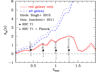
Figure 10: The amplitude of the intrinsic alignment at each tomographic bin derived from our cosmic shear power spectrum analysis (filled circles) and from the combined analysis with Planck (open triangles), in which the NLA model is assumed [see equation (40)]. For comparison, we plot IA amplitudes extrapolated from the luminosity-dependent IA signals of bright red galaxies by Joachimi et al. (2011) (thick) and Singh et al. (2015) (thin) assuming that only red galaxies have IA signals (solid) or all galaxies have comparable IA signals (dashed).

6.2.5 Intrinsic alignment modeling

In our fiducial analysis, we adopt the NLA model to model intrinsic alignment contributions to cosmic shear power spectra (see Section 5.4). We include two parameters in the nested sampling analysis, the overall amplitude $A_{\rm IA}$ and the power-law index of the redshift dependence of $A_{\rm IA}$, $\eta_{\rm eff}$, which are marginalized over when deriving cosmological constraints.

We test the robustness of our cosmological constrains by adopting IA models that are different from our fiducial model described above. First, when the IA contribution is completely ignored, i.e., $A_{\rm IA}$ is fixed to $0$ in the nested sampling analysis, the $S_{8}$ value decreases by $\sim 0.5\sigma$ (see e.g., Table 7). This is because the negative contribution of the GI term to the measured cosmic shear power spectrum is ignored in this case. Next, when the IA amplitude $A_{\rm IA}$ is free but the power-law index of the redshift evolution, $\eta_{\rm eff}$, is fixed to $3$, which is a plausible value of $\eta_{\rm eff}$ assuming that only red galaxies have IA signals (see Section 5.4), we find no significant change of the best-fit $S_{8}$ value or $\Omega_{\rm m}$ value.

We now discuss the validity of the IA model parameters derived in the fiducial nested sampling analysis. We find that the IA amplitude is consistent with zero, $A_{\rm IA}=0.38\pm 0.70$, for the pivot redshift $z_{0}=0.62$. As a further check, when we adopt stacked photo-$z$ PDFs from several different photo-$z$ codes (see Section 6.2.2), we find slightly positive values of IA signals for some codes, $1.00\pm 0.61$ for Ephor AB, $0.50\pm 0.69$ for MLZ, $0.62\pm 0.62$ for Mizuki, $1.25\pm 0.54$ for NNPZ, $0.55\pm 0.67$ for Frankenz, and $0.78\pm 0.61$ for DEmP, although the significance of non-zero $A_{\rm IA}$ is not high in any case. This may indicate that constraint on the IA amplitude is more sensitive to the photo-$z$ uncertainty than that on $S_{8}$.

Together with derived constraints on the redshift dependence, $\eta_{\rm eff}$, we derive $A_{\rm IA}$ amplitudes and their 1$\sigma$ errors for individual tomographic bins as

$$A_{\rm IA}(z)=A_{\rm IA}((1+\langle z\rangle)/(1+z_{0}))^{\eta_{\rm eff}}$$ (40)

where $\langle z\rangle$ is the weighted average of source redshifts in each bin. Figure 10 shows the results of $A_{\rm IA}(z)$ derived from our nested sampling. We do not find significant redshift evolution of $A_{\rm IA}$. We compare this redshift evolution with the extrapolation of IA amplitudes from the luminosity-dependent IA signals of bright red galaxies (Joachimi et al., 2011; Singh et al., 2015). We consider two cases, one in which only red galaxies have IA signals and the other in which all galaxies including blue galaxies have comparable IA signals. The details of the model are given in Section 5.4. Figure 10 shows that our results are more consistent with the former model. This result is consistent with the idea that blue galaxies do not make a significant contribution to the overall amplitude of the observed IA signal. While tidal torquing aligns blue galaxies with large-scale structure, the IA of blue galaxies has not yet been detected in observations (Joachimi et al., 2015). In either case, more accurate measurements of cosmic shear signals are necessary for further analysis of the IA. Our conclusion here is that the IA signals from our fiducial analysis appear to be reasonable. We will discuss the IA result when combining HSC first year cosmic shear with Planck in Section 6.4.

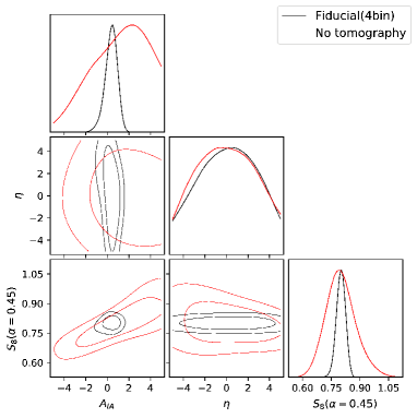
Figure 11: Joint constraints and marginalized one-dimensional posteriors for the amplitude of the intrinsic alignment $A_{\rm IA}$, the power-law index of the redshift evolution, $\eta_{\rm eff}$, and $S_{8}$ in our fiducial four tomographic redshift bin analysis are compared with those from non-tomographic cosmic shear analysis. The contours represent 68% and 95% credible levels. It clearly demonstrates that the lensing tomography helps break the degeneracy between $A_{\rm IA}$ and $S_{8}$.

Finally, we show that the tomographic analysis helps break the degeneracy between $S_{8}$ and the IA parameters. Figure 11 shows the joint constraints on the amplitude parameter of intrinsic alignment $A_{\rm IA}$, the power-law index of the redshift evolution $\eta_{\rm eff}$, and $S_{8}$ with and without tomography. It clearly demonstrates the power of lensing tomography to break the degeneracy between $A_{\rm IA}$ and $S_{8}$.

6.2.6 Internal consistency among different redshift and multipole bins

In our fiducial analysis, we adopt four tomographic bins to constrain the redshift dependence of cosmic shear power spectra. The comparison of our cosmological results among these tomographic bins serves as an important internal consistency check (e.g., Efstathiou & Lemos, 2018; Köhlinger et al., 2018). For this purpose, we exclude one photo-$z$ bin at a time and see whether the results are consistent with the fiducial one as shown in the bottom-left panels of Figures 8 and 9. We find that the results of $S_{8}$ are consistent within 0.3$\sigma$ when any one of the four tomographic bins is excluded (see e.g., Table 7). This indicates that our $S_{8}$ results do not significantly rely on the cosmic shear power spectrum at any specific redshift bin. In contrast, we find that the shift of the best-fit $\Omega_{\rm m}$ value is relatively larger than $S_{8}$. In particular, when the measurement at mid-lower redshift bin is excluded, the best-fit $\Omega_{\rm m}$ value shifts to a value $\sim 1\sigma$ higher, although the error on $\Omega_{\rm m}$ also increases by 60%. This suggests that the constraint on $\Omega_{\rm m}$ is driven by the relative amplitudes of cosmic shear power spectra between low and high redshift bins.

As done in Section 6.1, we can use the HSC mock shear catalogs to see whether the large shift in the best-fit $\Omega_{\rm m}$ value when excluding a single redshift bin is simply explained by a statistical fluctuation. We find that 9 out of 100 mock realizations show more than a $1\sigma$ shift of the best-fit $\Omega_{\rm m}$ value by excluding the measurement at the mid-lower redshift bin. Thus we conclude that the observed large shift of $\Omega_{\rm m}$ value can be explained by a $<2\sigma$ statistical fluctuation.

We also check the internal consistency among different multipole bins. We first split the fiducial multipole range ($300<\ell<1900$) into half, i.e., $300<\ell<800$ (a lower-half bin) and $800<\ell<1900$ (a higher-half bin) as shown in the middle-right panels of Figures 8 and 9. We find no significant shift of either $S_{8}$ or $\Omega_{\rm m}$. Although the measurements at the higher-half $\ell$ prefer higher values of $\Omega_{\rm m}$, once the larger statistical error is taken into account the significance is less than 1$\sigma$. Next we extend the upper limit of the $\ell$ range from $1900$ to $3500$ and repeat the nested sampling analysis. We find that neither best-fit values of $S_{8}$ and $\Omega_{\rm m}$ change significantly, although this modification leads to a 10% smaller statistical error for $S_{8}$ and 20% smaller error for $\Omega_{\rm m}$ than our fiducial case. This indicates that our result is insensitive to the choice of the multipole range and the small-scale physics such as one-halo term of the intrinsic alignment and baryon physics. This test suggests that our fiducial choice of the multipole range of $300<\ell<1900$ is conservative.

6.2.7 Covariance

In our analysis we use an analytic model of the covariance matrix (Section 5.3) that includes the dependence of the covariance matrix on cosmological parameters in the likelihood function [equation (33)]. Here we check how the results differ when the covariance is fixed to that in the best-fit cosmology, as has been assumed in most previous cosmic shear analyses. We find that both $S_{8}$ and $\Omega_{\rm m}$ agree within 20% of the statistical uncertainty, and sizes of the errors also agree within 10%. This indicates that the effect of the cosmology dependence of the covariance is subdominant in our analysis.

6.2.8 Summary of the robustness checks

The robustness checks presented above indicate that our results are indeed robust against various systematics and modeling choices?. Among others, the most significant sources of possible systematics are photo-$z$ uncertainties, intrinsic alignment modeling, and the effect of baryonic physics on the matter power spectrum, which can shift the best-fit values of $S_{8}(\alpha=0.45)$ by up to $\sim 0.6\sigma$ of the statistical errors in most extreme cases examined in this paper. We find that constraints on $\Omega_{\rm m}$ are more sensitive to various systematics in that they shift the best-fit values up to $\sim 1\sigma$ of the statistical errors. This is because these systematics tend to move the best-fit values along the degeneracy direction in the $\Omega_{\rm m}$-$\sigma_{8}$ plane. In addition, we conduct internal consistency checks among different redshift and multipole bins, and find no sign of systematics.

6.3 Consistency between HSC cosmic shear and CMB data

We evaluate the consistency between our HSC cosmic shear measurements and CMB datasets from both Planck and WMAP9. The consistency between different datasets is often judged with the following Bayesian evidence ratio (Marshall et al., 2006):

$$R=\frac{P(\mathbf{D_{1},D_{2}}|{\rm M})}{P(\mathbf{D_{1}}|{\rm M})P(\mathbf{D_{2}}|{\rm M})},$$ (41)

where $D_{1}$ and $D_{2}$ denote the two datasets and $M$ indicates the cosmological model (either $\Lambda$CDM or $w$CDM). The numerator is the evidence that the two datasets $D_{1}$ and $D_{2}$ share the same cosmological parameters in a given model $M$, while the denominator is the evidence that the two datasets have different cosmological parameters in the model $M$. A positive (negative) value of $\log R$ would indicate that the two datasets are (in)consistent.

Table 8: Bayesian evidence ratios $R$ and the differences of log-likelihoods at the maximum a posteriori point $Q_{\rm DMAP}$ in different combinations of datasets based on the $\Lambda$CDM or $w$CDM cosmology. The values listed here indicate that all dataset combinations are consistent.

model	datasets	$\log R$	$Q_{\rm DMAP}$
$\Lambda$CDM	HSC + Planck	3.7	2.4
$\Lambda$CDM	HSC + WMAP9	4.1	1.5
$w$CDM	HSC + Planck	5.3	0.5

Table 8 lists values of $\log R$ in different combinations of datasets and cosmological models. We obtain a positive value of $\log R$ for HSC and Planck in the $\Lambda$CDM model, which indicates that the tension in the two datasets, if any, does not rise to a significant level. We also find that the value of $R$ is even larger for HSC and WMAP combinations and also for the $w$CDM model. In all the cases examined here, the Bayesian evidence ratio does not signal inconsistency between HSC cosmic shear measurements and Planck and WMAP9 CMB datasets.

As a further test, we employ another criterion of consistency using differences of log-likelihoods at the maximum a posteriori (MAP) point $\theta_{p}$ in parameter space (Raveri & Hu, 2018)

$$Q_{\rm DMAP}=-2\ln{\cal L}_{12}(\theta_{p}^{12})+2\ln{\cal L}_{1}(\theta_{p}^{1})+2\ln{\cal L}_{2}(\theta_{p}^{2}).$$ (42)

This can be interpreted as the difference of $\chi^{2}$ values $\Delta\chi_{\rm eff}^{2}=\chi^{2}_{\rm eff,12}-\chi^{2}_{\rm eff,1}-\chi^{2}_{\rm eff,2}$ where $\chi^{2}_{\rm eff,i}$ is defined as $-2\ln{\cal L}_{i}(\theta_{p}^{i})$. This criterion was also used as a consistency check by the recent Planck 2018 paper (Planck Collaboration et al., 2018). We show the values of $Q_{\rm DMAP}$ in Table 8. In this calculation, we use the covariance assuming Planck cosmology. The statistic $Q_{\rm DMAP}$ is expected to follow a $\chi^{2}$ distribution with $N_{\rm eff}^{1}+N_{\rm eff}^{2}-N_{\rm eff}^{12}$, which becomes about 2 degrees of freedom (Raveri & Hu, 2018). We find $Q_{\rm DMAP}=2.4$ for HSC and Planck, which corresponds to a p-value of $0.30$. In conclusion, we do not find any signs of significant inconsistency between HSC and Planck and WMAP9 CMB datasets for both the $\Lambda$CDM and $w$CDM models.

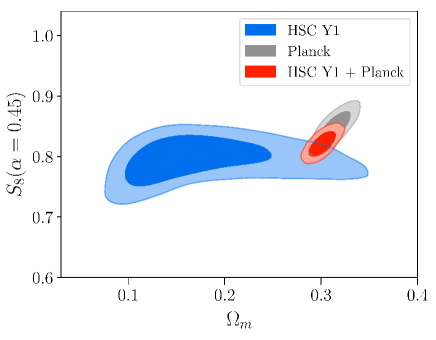
Figure 12: Marginalized constraints in the $\Omega_{\rm m}$-$S_{8}(\alpha=0.45)$ plane for HSC, Planck, and their joint analysis. The contours represent 68% and 95% credible levels. The contours for the HSC alone and Planck alone are same as those plotted in Figure 5.

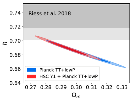
Figure 13: Marginalized constraints in the $\Omega_{\rm m}$-$h$ plane in the $\Lambda$CDM model for Planck alone and Planck + HSC Y1. The contours represent 68% and 95% credible levels. We also show the local Hubble constraint measurement by Riess et al. (2018) for comparison.

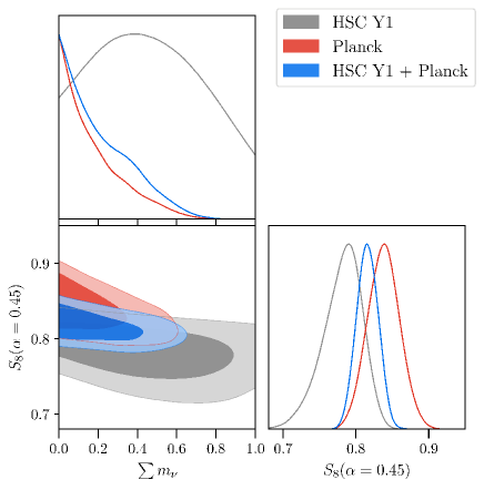
Figure 14: Marginalized constraints and one-dimensional posteriors of the sum of neutrino masses $\sum m_{\nu}$ and $S_{8}(\alpha=0.45)$ from HSC, Planck, and their joint analysis. The contours represent 68% and 95% credible levels. Increasing $\sum m_{\nu}$ decreases $S_{8}$.

6.4 Joint constraints combining HSC with external datasets

Since we do not see any hints for inconsistencies between HSC and Planck, we now conduct a joint cosmology analysis by combining the HSC cosmic shear and Planck 2015 results. In addition, we present results combining the distance measurements using a set of baryonic acoustic oscillations (BAOs) and 740 Type Ia supernovae (SNe) via the Joint Lightcurve Analysis (JLA) data (Betoule et al., 2014). The BAO dataset includes the measurements of angular diameter distances from the 6dF Galaxy Survey (Beutler et al., 2011), the SDSS DR7 Main Galaxy Sample (Ross et al., 2015), and BOSS LOWZ and CMASS DR12 sample (Alam et al., 2017). In this subsection, we take into account the lower bound of the absolute sum of neutrino mass, $\sim 0.06$ eV to match the fiducial setup in Planck Collaboration et al. (2016).

Figure 12 shows marginalized constraints on $\Omega_{\rm m}$ and $S_{8}$ from HSC and Planck in the flat $\Lambda$CDM model. When combining HSC and Planck, constraints on $S_{8}$ and $\Omega_{\rm m}$ both improve, to $0.821\pm 0.017$ and $0.301\pm 0.010$, respectively, compared to Planck alone (Planck Collaboration et al., 2016) where $S_{8}=0.848\pm 0.024$ and $\Omega_{\rm m}=0.315\pm 0.013$. Since the well-determined CMB peak locations are highly sensitive to the combination of $\Omega_{\rm m}h^{3}$ (Percival et al., 2002), lower $\Omega_{\rm m}$ slightly increases the Hubble parameter $H_{0}$ to $68.36\pm 0.81$ km/s from the joint analysis of HSC and Planck, as shown in Figure 13. The reported 3.7$\sigma$ tension of $H_{0}$ between Planck and the local measurement (Riess et al., 2018) reduces to 3.1$\sigma$ by adding our cosmic shear measurement. The difference is still present, albeit at a slightly smaller significance.

Figure 14 shows marginalized constraints from HSC, Planck, and their combination when the sum of neutrino masses $\sum m_{\nu}$ is allowed to vary. The constraint on $\sum m_{\nu}$ from the HSC cosmic shear measurement alone is very weak with the peak of the posterior around 0.45 eV, for the reasons described in Section 6.2.3. Increasing the sum of the neutrino mass damps the amplitude of linear matter fluctuations and thus decreases the constraints on $S_{8}$ for both Planck and HSC. Since the HSC cosmic shear constraints favor a higher $\sigma_{8}$ value than that from the Planck data as shown in Figure 5, we cannot expect that combining the HSC and Planck constraints improves the neutrino mass constraint. For this reason, the posterior distribution of $\sum m_{\nu}$ does not significantly change between Planck and the joint constraint from HSC and Planck, although a slight increase of the probability at larger $\sum m_{\nu}$ is seen when the HSC constraint is added.

We obtain the intrinsic alignment amplitude of $A_{\rm IA}=0.73\pm 0.46$ when combining HSC cosmic shear with Planck. The amplitude is slightly higher than the value from the HSC cosmic shear analysis alone, $A_{\rm IA}=0.38\pm 0.70$. The intrinsic alignment amplitudes of individual redshift bins shown in Figure 10 indicate that our result is consistent with the hypothesis that only red galaxies have significant IA signals (see Section 5.4 for more details).

When varying the baryonic feedback parameter [see equation (28)], we obtain $A_{B}=1.1\pm 0.8$ from the joint analysis of the HSC cosmic shear and Planck, which appears to slightly prefer the presence of baryon feedback effects on the matter power spectrum. This is because baryon feedback increases the HSC-inferred values of $S_{8}$ and $\Omega_{\rm m}$, making them more consistent with the Planck best-fit values, as discussed in Section 6.2.4. We check whether the preference of the model including the baryon feedback parameter is significant or not using the following Bayesian evidence ratio

$$K_{B}(\mathbf{D})=\frac{P(\mathbf{D}|\Lambda{\rm CDM}+A_{B})}{P(\mathbf{D}|\Lambda{\rm CDM})}.$$ (43)

The Bayesian evidence $P(\mathbf{D}|{\rm M})$ indicates the probability of obtaining dataset $\mathbf{D}$ in the model ${\rm M}$

$$P(\mathbf{D}|{\rm M})=\int\mathbf{dp}P(\mathbf{D}|\mathbf{p},{\rm M})P(\mathbf{p}|{\rm M}),$$ (44)

where $P(\mathbf{D}|\mathbf{p},{\rm M})$ is the likelihood and $P(\mathbf{p}|{\rm M})$ is the prior of the parameter set of $\mathbf{p}$. A value of $K_{B}$ larger than unity would indicate that the model with the baryon feedback parameter is preferred. The substantial evidence of the preference of the model with the baryon feedback parameter is found when $K_{B}>\sqrt{10}$ and strong evidence when $K_{B}>10$, based on Jeffreys’ scale, and vice versa. However, we find $K_{B}=0.46$, which indicates that there is no preference for the model including the baryon feedback parameter, and the improvement in the fit to the data is not significant enough to justify addition of another parameter.

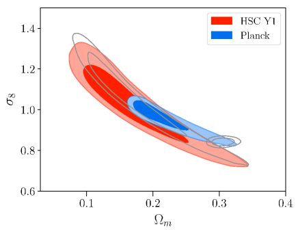
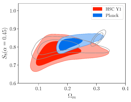
Figure 15: Same as Figure 5, but for the constraints from HSC and Planck in the $w$CDM model. For reference, the constraints in the fiducial $\Lambda$CDM model are shown by gray contours.

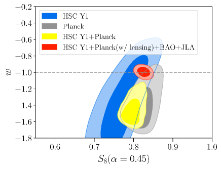
Figure 16: Marginalized constraints in the $S_{8}(\alpha=0.45)$-$w$ plane for the $w$CDM model from HSC, Planck, and their joint analysis. The contours represent 68% and 95% credible levels.

6.5 Cosmological constraints in the $w$CDM model

Next we allow the dark energy equation of state constant $w$ to be a free parameter in our model, instead of our fiducial choice of fixing its value to $-1$. We find that $S_{8}(\alpha=0.45)=0.773^{+0.043}_{-0.038}$ and $\Omega_{\rm m}=0.163^{+0.079}_{-0.047}$. Figure 15 shows marginalized constraints in the $\Omega_{\rm m}$-$\sigma_{8}$ and $\Omega_{\rm m}$-$S_{8}(\alpha=0.45)$ planes. Adding $w$ as a model parameter significantly degrades constraints on $S_{8}$ compared with the $\Lambda$CDM case. This indicates that $w$ is not well- constrained from the cosmic shear analysis alone.

The degeneracy between $S_{8}$ and $w$ is clearly seen in Figure 16, which shows the constraints in the $S_{8}$-$w$ plane. The constraint on $w$ is $w=-1.37^{+0.43}_{-0.37}$ from HSC cosmic shear measurements alone. We find that both HSC and Planck prefer $w<-1$, leading to their joint constraint of $w=-1.45^{+0.16}_{-0.10}$, i.e., 3$\sigma$ deviation from $w=-1$. The similar deviation was found also in the previous lensing surveys by Joudaki et al. (2017b); DES Collaboration et al. (2017). As discussed in Planck Collaboration et al. (2016), this comes from the strong degeneracy between $w$ and $h$. When we add the BAOs and SNe data, we obtain $w=-1.006\pm 0.044$. This constraint on $w$ is similar to that from Planck+BAOs+SNe without the HSC result, $w=-1.012\pm 0.046$ (Planck Collaboration et al., 2016; Alam et al., 2017).

We evaluate the possible preference for the $w$CDM model over the $\Lambda$CDM model based on the Bayes factor similar to equation (43)

$$K_{w{\rm CDM}}(\mathbf{D})=\frac{P(\mathbf{D}|w{\rm CDM})}{P(\mathbf{D}|\Lambda{\rm CDM})}.$$ (45)

We obtain $K_{w{\rm CDM}}=0.73\pm 0.05$ from our HSC cosmic shear analysis, which indicates that there is no preference for $w\neq-1$ from the cosmic shear alone. When combining HSC with Planck, the value of $K_{w{\rm CDM}}$ increases to 2.7, which indicates that the $w$CDM model is favored, although the significance is small. When combining HSC with Planck including lensing and with BAOs and SNe, however, $K_{w{\rm CDM}}$ decreases to 0.091, indicating that the $w$CDM model is not preferred. This is not surprising given that our best fit $w$CDM model when including all the probes was not significantly different from our fiducial choice of dark energy being a cosmological constant, i.e. $w=-1$.

7 Summary and conclusions

We have presented results of the cosmic shear power spectrum analysis using the HSC first-year data over 137 deg² of sky. The exquisite depth and image quality of the HSC survey images allow us to construct a source galaxy sample with an effective number density of $16.5$ arcmin^-2 even after conservative cuts for constructing the accurate shear catalog (Mandelbaum et al., 2018a) as well as the redshift cut of $0.3\leq z\leq 1.5$ for the tomographic analysis.

We have measured cosmic shear power spectra from the HSC first-year shear catalog using the pseudo-$C_{\ell}$ method that corrects for the non-uniform mask effect due to the survey geometry, the bright star masks, and the non-uniformity of the number density of sources. Using realistic HSC mock shear catalogs, we have demonstrated that this method separates E- and B-modes and recovers input spectra in an unbiased way.

The measured tomographic cosmic shear power spectra have a total signal-to-noise ratio of 16, whereas the B-mode power spectra are consistent with zero within the multipole range $300\leq\ell\leq 1900$. We fit the spectra using a model that includes contributions from intrinsic alignments of galaxies, as well as seven additional nuisance parameters to account for shape measurement errors and photo-$z$ errors. We use an analytic model for the covariance matrix, whose accuracy has also been tested against the HSC mock shear catalogs. We have found that our model fits the measured cosmic shear power spectra quite well, with a minimum $\chi^{2}$ of 45.4 for 56.9 degrees of freedom for our fiducial $\Lambda$CDM model.

Our cosmological constraints are well encapsulated by constraints on the parameter $S_{8}=\sigma_{8}(\Omega_{\rm m}/0.3)^{\alpha}$, with $\alpha=0.45$ being the best choice for our case. Assuming a flat $\Lambda$CDM model, we have found $S_{8}(\alpha=0.45)=0.800^{+0.029}_{-0.028}$ and $S_{8}(\alpha=0.5)=0.780^{+0.030}_{-0.033}$. When the dark energy equation of state $w$ is allowed to deviate from $-1$, the constraint on $S_{8}$ is degraded to $S_{8}(\alpha=0.45)=0.773^{+0.043}_{-0.038}$. The dark energy equation of state is not very well constrained from the HSC cosmic shear analysis alone, $w=-1.37^{+0.43}_{-0.36}$. Our constraints on $S_{8}$ agree with other recent cosmic shear analysis results (Hildebrandt et al., 2017; Köhlinger et al., 2017; Troxel et al., 2018b) as well as results of extended analyses including galaxy-galaxy lensing (Joudaki et al., 2018; van Uitert et al., 2018; DES Collaboration et al., 2017; Yoon et al., 2018). The 3.6% fractional constraint on $S_{8}$ represents one of the tightest constraints on $S_{8}$ from cosmic shear analyses conducted to date.

We have carefully checked the consistency between our HSC cosmic shear results and CMB datasets both for Planck 2015 and WMAP9. Both the results of the Bayesian evidence ratio and the difference of log-likelihoods at the maximum a posteriori point indicate that the HSC cosmic shear results and these CMB datasets are consistent with each other. The best-fit value of $S_{8}$ from the HSC cosmic shear analysis is also consistent within 2$\sigma$ with those from Planck 2015 and WMAP9.

To check the robustness of our results, we have conducted a number of systematics tests and tests for our sensitivity to modeling assumptions such as additional photo-$z$ uncertainties, the uncertainty of IA modeling, and the effect of baryon physics on the matter power spectrum. We find that our results are robust against these systematics in that they can shift the best-fit values of $S_{8}$ by no more than $\sim 0.6\sigma$ of the statistical errors. We have also found our cosmological results are consistent among different redshift and multipole bins.

In our cosmological analysis we simultaneously fit the IA amplitude as well as its redshift evolution. The best-fit IA amplitude at the pivot redshift of $z_{0}=0.62$ and its 1$\sigma$ error is found to be $A_{\rm IA}=0.38\pm 0.70$, which indicates that the IA amplitude is consistent with zero. We have found that the redshift evolution of $A_{\rm IA}$ is weak. These results are consistent with a model that the IA amplitude is dominated by that of red galaxies, although this conclusion is based on the extrapolation of IA amplitude scalings that are calibrated using luminous red galaxies. We have also confirmed that our constraints on $S_{8}$ are insensitive to the priors we use on the parameters of our IA model.

While our results are statistically consistent with the Planck 2015 results, both the best-fit values of $S_{8}(\alpha=0.45)=0.800^{+0.029}_{-0.028}$ and $\Omega_{\rm m}=0.162^{+0.086}_{-0.044}$ are lower than the Planck result. Such lower best-fit values of $S_{8}$ and $\Omega_{\rm m}$ are also found in other recent weak lensing analyses (e.g., DES Collaboration et al., 2017). Although our consistency and mock analysis indicates that these lower values could just be a statistical fluctuation, there is a possibility that these lower values originate from systematic effects that are unaccounted for in our current cosmic shear analysis, or more interestingly, from a possible failure of our fiducial neutrino mass-free $\Lambda$CDM model. For instance, our robustness tests have shown that systematic errors and modeling choices tend to have a larger impact on $\Omega_{\rm m}$ than on $S_{8}$, which could imply that the low $\Omega_{\rm m}$ of our result might partly be due to additional systematic errors. However, it is also possible that the lower values of $S_{8}$ and $\Omega_{\rm m}$ have a physical origin. The lower best-fit value of $\Omega_{\rm m}$ seen in our measurements of the HSC cosmic shear power spectra could be due to a slower redshift evolution of density fluctuations than predicted by the $\Lambda$CDM model with Planck best-fit cosmological parameters. Hence it is of great importance to improve constraints from weak lensing in order to discriminate between these possibilities.

This paper presents cosmological results from the HSC first-year data. When the HSC survey is completed in $\sim 2019$, we will have roughly seven times more area for the cosmic shear analysis. In addition to increased area, there is room for improvement in several ways. For instance, we have constructed the HSC first-year shear catalog adopting a number of conservative cuts on galaxy magnitudes, PSF sizes, and signal-to-noise ratios. By improving shear measurement techniques, we can increase the fraction of galaxies that we can use for the cosmic shear analysis. While we conservatively limit the multipole range to $\ell<1900$, we can extend the analysis to higher multipoles once the intrinsic alignment at small scales and the modification of the matter power spectrum due to baryon physics are understood better. We plan to continue to improve photo-$z$ measurements in the HSC survey, both by increasing a sample of galaxies with spectroscopic redshifts for calibrations and by implementing new techniques such as clustering redshifts. Our first-year cosmic shear analysis suggests that with the increased area and continued improvements in analysis methodology, the final HSC weak lensing analysis has the potential to provide a stringent test of the concordance cosmological model.

We thank the referee, Catherine Heymans, for very useful comments and suggestions. We thank Michael Troxel for kindly providing the outputs of nested sampling with DES Y1 likelihoods. We also thank Ryuichi Takahashi, Chihway Chang, David Alonso for their feedback that improved the quality of the paper. Our likelihood code is partly based on the likelihood code from Köhlinger et al. (2017), which is publicly available at https://bitbucket.org/fkoehlin/kids450_qe_likelihood_public.

This work was supported in part by World Premier International Research Center Initiative (WPI Initiative), MEXT, Japan, JSPS KAKENHI Grant Number JP15H03654, JP16K17684, JP16H01089, JP17H06599, JP18H04348, JP18K03693, JP18H04350, MEXT Grant-in-Aid for Scientific Research on Innovative Areas (JP15H05887, JP15H05892, JP15H05893, JP15K21733), and JST CREST Grant Number JPMJCR1414. HMi and MSi are supported by the Jet Propulsion Laboratory, California Institute of Technology, under a contract with the National Aeronautics and Space Administration. RMa is supported by the Department of Energy Cosmic Frontier program, grant DE-SC0010118.

Data analysis were in part carried out on PC cluster at Center for Computational Astrophysics, National Astronomical Observatory of Japan. Numerical computations were in part carried out on Cray XC30 at Center for Computational Astrophysics, National Astronomical Observatory of Japan.

The Hyper Suprime-Cam (HSC) collaboration includes the astronomical communities of Japan and Taiwan, and Princeton University. The HSC instrumentation and software were developed by the National Astronomical Observatory of Japan (NAOJ), the Kavli Institute for the Physics and Mathematics of the Universe (Kavli IPMU), the University of Tokyo, the High Energy Accelerator Research Organization (KEK), the Academia Sinica Institute for Astronomy and Astrophysics in Taiwan (ASIAA), and Princeton University. Funding was contributed by the FIRST program from Japanese Cabinet Office, the Ministry of Education, Culture, Sports, Science and Technology (MEXT), the Japan Society for the Promotion of Science (JSPS), Japan Science and Technology Agency (JST), the Toray Science Foundation, NAOJ, Kavli IPMU, KEK, ASIAA, and Princeton University. This paper makes use of software developed for the Large Synoptic Survey Telescope. We thank the LSST Project for making their code available as free software at http://dm.lsst.org

The Pan-STARRS1 Surveys (PS1) have been made possible through contributions of the Institute for Astronomy, the University of Hawaii, the Pan-STARRS Project Office, the Max-Planck Society and its participating institutes, the Max Planck Institute for Astronomy, Heidelberg and the Max Planck Institute for Extraterrestrial Physics, Garching, The Johns Hopkins University, Durham University, the University of Edinburgh, Queen’s University Belfast, the Harvard-Smithsonian Center for Astrophysics, the Las Cumbres Observatory Global Telescope Network Incorporated, the National Central University of Taiwan, the Space Telescope Science Institute, the National Aeronautics and Space Administration under Grant No. NNX08AR22G issued through the Planetary Science Division of the NASA Science Mission Directorate, the National Science Foundation under Grant No. AST-1238877, the University of Maryland, and Eotvos Lorand University (ELTE) and the Los Alamos National Laboratory.

Based in part on data collected at the Subaru Telescope and retrieved from the HSC data archive system, which is operated by Subaru Telescope and Astronomy Data Center at National Astronomical Observatory of Japan.

Appendix A Pseudo-$C_{\ell}$ method in the flat-sky approximation and the test with mock shear catalogs

A.1 Formalism

Following the methodology developed in Hikage et al. (2011), here we provide a detailed description of the pseudo-$C_{\ell}$ method that we adopt for unbiased measurements of cosmic shear power spectra from the HSC first-year shear catalog. Throughout the paper we use a flat-sky approximation because the curvature effect on each disjoint patch of the current HSC survey data is negligible compared to the statistical errors. We define the observed shear field $\bm{\gamma}^{\rm(obs)}$ as a sum of weighted ellipticities at sky pixel position $\bm{\theta}$, after correcting for the shape bias and responsivity [equation (2)]. This shear field is related to the true shear field as

$$\bm{\gamma}^{\rm(obs)}(\bm{\theta})=W(\bm{\theta})\bm{\gamma}^{\rm(true)}(\bm{\theta}).$$ (46)

The mask (weight) field $W({\bm{\theta}})$ is computed as a sum of source weights $w_{i}$ within each pixel using a nearest neighbor assignment scheme. The observed shear field is decomposed into an E-mode (even parity) and B-mode (odd parity) in Fourier space as

$$\tilde{E}_{\bm{\ell}}\pm i\tilde{B}_{\bm{\ell}}=\int\bm{d\theta}\bm{\gamma}(\bm{\theta})e^{i(\bm{\ell\cdot\theta}\pm 2\varphi_{\bm{\ell}})},$$ (47)

where $\bm{\ell}$ denotes the two-dimensional harmonic vector, $\varphi_{\bm{\ell}}$ is the angle of $\bm{\ell}$, and the and the multipole $\ell$ corresponds to the angular scale $\theta=\pi/\ell$. In practice, we consider a square boundary to cover each of the separate fields of HSC data to perform the Fourier transform. The angular scale of the survey boundary is set to be 720 arcmin for XMM, WIDE12H, and HECTOMAP, 900 arcmin for GAMA09H and VVDS, and 1080 arcmin for GAMA15H. The number of pixels $N_{\rm pix}$ is set to be $1024^{2}$ for all of the fields. After Fourier-transforming the observed (weighted) shear field, we obtain the shear field convolved with the mask field as

$$(\tilde{E}_{\bm{\ell}}\pm i\tilde{B}_{\bm{\ell}})^{\rm(obs)}=\int\frac{\bm{d\ell}^{\prime}}{(2\pi)^{2}}(\tilde{E}_{\bm{\ell}^{\prime}}\pm i\tilde{B}_{\bm{\ell}^{\prime}})^{\rm(true)}\tilde{W}_{\bm{\ell-\ell}^{\prime}}e^{\pm 2i(\varphi_{\bm{\ell^{\prime}\ell}})},$$

where $\varphi_{\bm{\ell\ell^{\prime}}}$ denotes the angle between vectors $\bm{\ell}$ and $\bm{\ell}^{\prime}$ and $\tilde{W}_{\bm{\Delta}\ell}$ is the Fourier transform of $W(\bm{\theta})$

$$\tilde{W}_{\bm{\Delta}\ell}=\int\bm{d\theta}W(\bm{\theta})e^{i\bm{\Delta\ell\cdot\theta}}.$$ (49)

We define the auto and cross spectra of E- and B-mode cosmic shear as

$$\langle X_{\bm{\ell}}Y^{*}_{\bm{\ell^{\prime}}}\rangle = \Omega_{\rm sky}\delta^{\rm K}_{\bm{\ell-\ell^{\prime}}}C_{\bm{\ell}}^{XY},$$ (50)

where $X_{\bm{\ell}}$ and $Y_{\bm{\ell}}$ denote the Fourier transform of E- and B-mode shear, respectively, $\delta^{\rm K}_{\bm{\ell}}$ is the Kronecker delta, and $\Omega_{\rm sky}$ is the sky area with non-zero $W(\bm{\theta})$. The power spectrum for the weighted field has mode coupling because of the presence of the weight field in real space. This coupling can expressed as

$${\cal C}_{\bm{\ell}}^{\rm(obs)}=\sum_{\bm{\ell}^{\prime}}\bm{M}_{\bm{\ell\ell^{\prime}}}F_{\ell}^{2}{\cal C}_{\bm{\ell}^{\prime}}^{\rm(true)}+\bm{N}_{\bm{\ell}}^{\rm(obs)},$$ (51)

where ${\cal C}_{\bm{\ell}}=(C_{\bm{\ell}}^{EE},C_{\bm{\ell}}^{BB},C_{\bm{\ell}}^{EB})$, $\bm{M}$ is convolution matrix, $F_{\ell}$ is the pixel window function as we use a pixelized map in the $\bm{\theta}$ space, and $\bm{N}_{\bm{\ell}}^{\rm(obs)}$ is the noise spectrum that is also convolved with the weight field. Non-zero components of the convolution matrix are given by

$$\bm{M}_{\bm{\ell\ell^{\prime}}}^{EE,EE}=\bm{M}_{\bm{\ell\ell^{\prime}}}^{BB,BB}=\frac{{\cal W}_{\bm{\ell-\ell^{\prime}}}^{\gamma\gamma}}{\Omega_{\rm sky}}\cos^{2}(2\varphi_{\bm{\ell\ell^{\prime}}}),$$ (52)

$$\bm{M}_{\bm{\ell\ell^{\prime}}}^{EE,BB}=\bm{M}_{\bm{\ell\ell^{\prime}}}^{BB,EE}=\frac{{\cal W}_{\bm{\ell-\ell^{\prime}}}^{\gamma\gamma}}{\Omega_{\rm sky}}\sin^{2}(2\varphi_{\bm{\ell\ell^{\prime}}}),$$ (53)

$$\bm{M}_{\bm{\ell\ell^{\prime}}}^{EB,EB}=\frac{{\cal W}_{\bm{\ell-\ell^{\prime}}}^{\gamma\gamma}}{\Omega_{\rm sky}}[\cos^{2}(2\varphi_{\bm{\ell\ell^{\prime}}})-\sin^{2}(2\varphi_{\bm{\ell\ell^{\prime}}})],$$ (54)

where ${\cal W}^{\gamma\gamma}_{\bm{\ell}}$ is the power spectrum of the weight field $W(\bm{\theta})$. The convolution with the mask generates apparent B-mode cosmic shear power spectrum which is leakage from the E-mode power spectrum, even if there is no intrinsic power in the B-mode as is the case for cosmic shear. We also account for the effect of the finite square boundary of each field to compute the full mode coupling matrix (Hikage et al., 2011). The mode coupling matrix is inverted after binning. To do so, we compute the binned dimensionless power spectrum as

$${\cal C}_{b}\equiv\frac{1}{N_{{\rm mode},b}}\sum_{\bm{\ell}}^{\ell\in\ell_{b}}P_{b\ell}C_{\bm{\ell}},$$ (55)

where $b$ is the label for the $\ell$ bin, $P_{b\ell}=\ell^{2}/2\pi$ and $N_{{\rm mode},b}$ is the number of modes in the bin, approximately given by

$$N_{{\rm mode},b}\simeq\frac{\Omega_{\rm sky}}{4\pi}(\ell_{b,{\rm max}}^{2}-\ell_{b,{\rm min}}^{2}).$$ (56)

The sum in the equation (55) runs over the $\ell$ modes in the given bin $b$.

The binned power spectrum with the mask correction is obtained by multiplying the inverse of the mode coupling matrix by the pseudo-spectrum

$${\cal C}_{b}^{\rm(true)}=\bm{M}_{bb^{\prime}}^{-1}\sum_{\bm{\ell}}^{|{\bm{\ell}}|\in\ell_{b}^{\prime}}P_{b^{\prime}\ell}(\bm{C}_{\bm{\ell}}^{\rm(obs)}-\langle\bm{N}_{\bm{\ell}}\rangle_{\rm MC}),$$ (57)

where

$$\bm{M}_{bb^{\prime}}=\sum_{\bm{\ell}}^{{\bm{\ell}}\in\ell_{b}}\sum_{\bm{\ell^{\prime}}}^{\bm{\ell^{\prime}}\in\ell_{b^{\prime}}}P_{b\ell}M_{\bm{\ell\ell^{\prime}}}Q_{\ell^{\prime}b^{\prime}},$$ (58)

with $Q_{\ell b}=2\pi/\ell^{2}$. In order to remove the shot noise effect, we randomly rotate orientations of individual galaxies to estimate the noise power spectrum $\bm{N}_{\ell}$. For accurate estimates of the noise power spectrum, we repeat this procedure 10000 times and use average noise spectrum $\langle\bm{N}_{\ell}\rangle_{\rm MC}$ over these realizations. This averaging allows us to subtract the shot noise contribution to the cosmic shear power spectrum accurately.

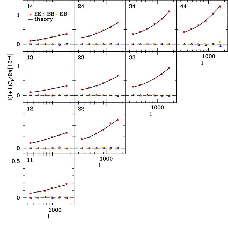
Figure 17: Tomographic cosmic shear power spectra (filled circles) measured on the HSC mock shear catalogs. The spectra are the weighted average of spectra for six disjoint fields (GAMA09H, GAMA15H, VVDS, WIDE12H, XMM, and HECTOMAP). The error-bars represent the 1$\sigma$ dispersion of the power spectra from the mock shear catalogs, divided by the square root of the number of mock realizations, $\sqrt{100}$. Input power spectra computed by equation (16) are shown as solid lines. We also plot BB (open triangles) and EB (crosses) spectra, which are consistent with zero.

A.2 Test with HSC mock shear catalogs

While the pseudo-$C_{\ell}$ method has been shown to recover input power spectra accurately (Hikage et al., 2011; Hikage & Oguri, 2016), we explicitly check the validity and accuracy of the pseudo-$C_{\ell}$ method for our analysis of the HSC first-year data by applying it to the HSC mock shear catalogs (Oguri et al., 2018). The mocks use realizations of cosmic shear from all-sky ray-tracing simulations of Takahashi et al. (2017). The cosmological model is flat $\Lambda$CDM with best-fit values as measured by WMAP9 (Hinshaw et al., 2013): $\Omega_{\rm m}=0.279$, $\Omega_{\rm b}=0.046$, $\Omega_{\Lambda}=0.721$, $h=0.7$, $n_{\rm s}=0.97$, and $\sigma_{8}=0.82$. In order to construct realistic mock shear catalogs, we start with the real HSC first-year shear catalog, and replace ellipticities of individual galaxies with mock ellipticity values while retaining the positions of these galaxies. Therefore the mock catalogs have exactly the same spatial inhomogeneity and mask patterns as do the real HSC first-year catalogs, and therefore are well suited for careful tests of the accuracy of the correction for masking effects implemented by the pseudo-$C_{\ell}$ method.

The mock ellipticity values include realistic noise properties as well as cosmic shear from the all-sky ray-tracing simulations. We take account of the redshift distribution of source galaxies by randomly assigning redshifts of individual galaxies from their photo-$z$ PDFs, using the MLZ code (see Oguri et al., 2018). In the mock catalogs, we also include the multiplicative bias $m$ by shifting shear values taken from the ray-tracing simulations by a factor of $1+m$. Since the analysis of the mock catalogs is conducted while the true HSC shape catalog is blinded (see Section 3.2), we artificially shift the values of $m$ by a factor of 1.3; this value is also kept blinded during the analysis of the mock catalogs, in order to maintain the blind nature of our analysis. We use 100 mock samples in each of the six disjoint fields.

Figure 17 shows tomographic cosmic shear power spectra of the mock catalogs, measured by the pseudo-$C_{\ell}$ method. The spectra are averaged over 100 mock samples, and also are averaged over the six disjoint fields weighted by the effective number of source galaxies, $\sum w_{i}$, in each field. The error represents the 1$\sigma$ scatter of measured power spectra from the mock catalogs divided by the square root of the number of mock realizations, $\sqrt{100}$. For comparison, we show the input cosmic shear power spectra computed by equation (16). We find that the power spectra measured using the pseudo-$C_{\ell}$ method agree with the input spectra quite well. The small deficit at $\ell\gtrsim 2000$ in measured power spectra relative to the model calculation originates from the limited angular resolution of the all-sky ray-tracing simulations that are used for constructing the mock shear catalogs. We also find that both B-mode auto and EB cross spectra are consistent with zero.

We compute the $\chi^{2}$ values to quantify the goodness of fit between the input (zero for B- and EB-modes) and measured spectra averaged over the mocks, and find 74 for EE-auto, 70 for BB-auto, 62 for EB for 60 degrees of freedom. The corresponding $p$-values are 0.10, 0.18, and 0.41, respectively. Measured power spectra with our pseudo-$C_{\ell}$ method are consistent with the input power spectra even for $1/\sqrt{100}$ smaller statistical errors than those expected for the HSC first-year shear catalog, indicating that the systematic error originating from the inaccuracy of the pseudo-$C_{\ell}$ method is well below 10% of the statistical error and therefore is negligibly small. Furthermore, we perform the nested sampling analysis on the average cosmic shear power spectra from the 100 mock shear catalogs to test whether the input values of key cosmological parameters are recovered by this nested sampling analysis. We find that $\Omega_{\rm m}=0.292\pm 0.014$, $\sigma_{8}=0.801\pm 0.020$, and $S_{8}(\alpha=0.5)=0.791\pm 0.005$, where these are the errors in the mean over the 100 mock realizations. These values agree with the input values of $\Omega_{\rm m}=0.279$, $\sigma_{8}=0.82$, and $S_{8}=0.791$ within the statistical errors.

Appendix B Analytic model of the covariance matrix

B.1 Justification for use of an analytic model

There are several different ways to estimate the covariance matrix. One class of methods are resampling techniques, including the bootstrap and jackknife methods, which allow us to derive a covariance matrix directly from the observational data. However, the covariance matrix derived by the resampling technique represents a noisy estimate of the true covariance matrix. This noise in the covariance matrix may affect the analysis in several ways, such as the unstable inversion of the covariance matrix and noise bias in derived constraints (e.g., Hartlap et al., 2007; Norberg et al., 2009; Friedrich et al., 2016). Furthermore, a covariance matrix derived from the data does not contain the so-called super-survey modes which affect both large- and small-scale covariance via mode-coupling (Takada & Hu, 2013). One can instead resort to $N$-body (ray-tracing) simulations to estimate covariance matrices (e.g., Jee et al., 2016). However, a technical challenge is how to include the dependence of covariance matrices on cosmological parameters, as this approach requires a large number of $N$-body simulations for each set of cosmological parameters. In this paper, we use the covariance matrix calculated using the so-called halo model (Cooray & Sheth, 2002), which has no issue with noise and also can include the cosmological parameter dependence. Below we describe our analytic model in detail, and then compare our model with the covariance matrix derived from realistic HSC mock shear catalogs.

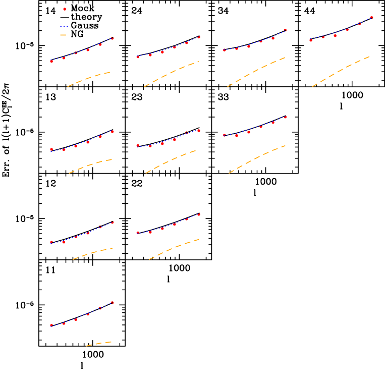
Figure 18: Comparison of 1$\sigma$ errors of the tomographic cosmic shear power spectra computed from the HSC mock shear catalogs (symbols), which correspond to the diagonal part of the covariance matrix, with the analytic model of the covariance described in the text (solid lines). The Gaussian and the non-Gaussian contributions including super-sample variance to the covariance matrix from the analytic model are shown by dotted and dashed lines, respectively. It is found that the contribution of the Gaussian term is dominant in the diagonal terms.

B.2 Analytic Model

As shown in equation (20), we decompose the covariance matrix of the cosmic shear power spectrum into three terms, the Gaussian term ${\rm Cov}^{\rm(G)}$, the non-Gaussian term ${\rm Cov}^{\rm(NG)}$, and the super-sample covariance ${\rm Cov}^{\rm(SSC)}$. The diagonal part of the Gaussian term of the covariance ${\rm Cov}^{\rm(G)}$ is given by

$${\rm Cov}^{\rm(G)}(C_{b}^{(ij)},C_{b^{\prime}}^{(i^{\prime}j^{\prime})}) = \frac{\delta_{bb^{\prime}}^{K}}{N_{{\rm mode},b}^{\rm eff}}\left[\hat{C}_{b}^{(ii^{\prime})}\hat{C}_{b}^{(jj^{\prime})}\right.$$ (59)

$$\left.+\hat{C}_{b}^{(ij^{\prime})}\hat{C}_{b}^{(i^{\prime}j)}\right],$$

where $b$ is a binning number of the multipole $\ell$, and $i$ and $j$ refer to tomographic bins. The effective number of Fourier modes in the $b$-th bin $N_{{\rm mode},b}^{\rm eff}$ is given by

$$N_{{\rm mode},b}^{\rm eff}=N_{\rm mode,b}w_{2}^{2}/w_{4}.$$ (60)

The factor $w_{2}^{2}/w_{4}$ represents the loss of modes due to pixel weighting, where $w_{k}$ is the $k$-th moment of the weight (Hivon et al., 2002) given by

$$w_{k}=\frac{1}{\Omega_{\rm sky}}\int\bm{d\theta}W^{k}(\bm{\theta}).$$ (61)

The binned spectra $\hat{C}_{b}^{ij}$ includes the shot noise

$$\hat{C}_{b}^{(ij)}=C_{b}^{(ij)}+N_{b}^{(ij)},$$ (62)

where $C_{b}^{(ij)}$ is the binned version of the model cosmic shear power spectrum computed from equation (16) and $N_{b}^{(ij)}$ is the binned shot noise spectrum, which is zero when $i\neq j$

$$N_{b}^{(ij)}=\delta_{ij}^{K}N_{b}^{(i)}.$$ (63)

As mentioned in Appendix A, we measure the shot noise spectrum $N_{b}^{(i)}$ directly from the data by randomly rotating shapes of individual galaxies. We note that in tomographic cosmic shear analysis the covariance between different tomographic bins is significant, because source galaxies with different redshifts share the same matter distribution along the line-of-sight.

The Gaussian covariance [equation (59)] can be further decomposed into the auto-term of cosmic shear power spectra, the cross-term between cosmic shear and shape noise spectra, and the auto-term of shape noise spectra. We write this explicitly as

$${\rm Cov}^{\rm(G)}_{SS}(C_{b}^{(ij)},C_{b}^{(i^{\prime}j^{\prime})}) = \frac{C_{b}^{(ii^{\prime})}C_{b}^{(jj^{\prime})}+C_{b}^{(ij^{\prime})}C_{b}^{(i^{\prime}j)}}{N_{{\rm mode},b}^{\rm eff}},$$ (64)

$${\rm Cov}^{\rm(G)}_{SN}(C_{b}^{(ij)},C_{b}^{(i^{\prime}j^{\prime})}) = \frac{1}{N_{{\rm mode},b}^{\rm eff}}\left[C_{b}^{(ii^{\prime})}N_{b}^{(jj^{\prime})}+N_{b}^{(ii^{\prime})}C_{b}^{(jj^{\prime})}\right.$$ (65)

$$\left.+C_{b}^{(ij^{\prime})}N_{b}^{(i^{\prime}j)}+N_{b}^{(ij^{\prime})}C_{b}^{(i^{\prime}j)}\right],$$

$${\rm Cov}^{\rm(G)}_{NN}(C_{b}^{(ij)},C_{b}^{(i^{\prime}j^{\prime})}) = \frac{N_{b}^{(ii^{\prime})}N_{b}^{(jj^{\prime})}+N_{b}^{(ij^{\prime})}N_{b}^{(i^{\prime}j)}}{N_{{\rm mode},b}^{\rm eff}}.$$ (66)

As discussed in Section 4.1, the shape noise covariance ${\rm Cov}^{\rm(G)}_{NN}$ estimated from the data shows small off-diagonal components of the covariance, mostly between neighboring multipole bins. In our analysis, we estimate ${\rm Cov}^{\rm(G)}_{NN}$ directly from the data using the shot noise simulations described in Appendix A, with 10000 Monte Carlo realizations of noise power spectra that are obtained by randomly rotating the ellipticities of individual galaxies, whereas we estimate ${\rm Cov}^{\rm(G)}_{SS}$ and ${\rm Cov}^{\rm(G)}_{SN}$ using equations (64) and (65).

The non-Gaussian term of cosmic shear power spectra ${\rm Cov}^{\rm(NG)}$ originates from the mode-coupling due to nonlinear gravitational evolution. This term was formulated in previous work (Cooray & Hu, 2001; Takada & Jain, 2003; Takada & Bridle, 2007), and can be expressed as

$${\rm Cov} {}^{\rm(NG)}(C_{b}^{(ij)},C_{b^{\prime}}^{(i^{\prime}j^{\prime})})=\frac{1}{\Omega_{\rm sky}}$$ (67)

$$\times\int_{|\mathbf{\ell}\in\ell_{b}|}\frac{\mathbf{d\ell}}{A(\ell_{i})}\int_{|\mathbf{\ell^{\prime}}\in\ell_{b}^{\prime}|}\frac{\mathbf{d\ell^{\prime}}}{A(\ell_{i}^{\prime})}T^{(iji^{\prime}j^{\prime})}(\mathbf{\ell},-\mathbf{\ell},\mathbf{\ell^{\prime}},-\mathbf{\ell^{\prime}})$$

$$\simeq \frac{1}{\Omega_{\rm sky}}T^{\rm(iji^{\prime}j^{\prime})}(\ell_{b},\ell_{b},\ell_{b^{\prime}},\ell_{b^{\prime}}),$$

where $\Omega_{\rm sky}$ is the observed sky area and $A(\ell_{i})\equiv\int_{|\mathbf{\ell}|\in\ell_{b}}\mathbf{d\ell}$. In the second line, we assume that the trispectrum within bins of $\ell$ is represented as

$$T^{(iji^{\prime}j^{\prime})}( \ell_{b} ,\ell_{b},\ell_{b}^{\prime},\ell_{b}^{\prime})$$ (68)

$$= \int_{0}^{\chi_{H}}d\chi\frac{q^{(i)}(\chi)q^{(j)}(\chi)q^{(i^{\prime})}(\chi)q^{(j^{\prime})}(\chi)}{f_{K}^{6}(\chi)}$$

$$\times T_{\delta}\left(\frac{\ell_{b}}{f_{K}(\chi)},\frac{\ell_{b}}{f_{K}(\chi)},\frac{\ell_{b}^{\prime}}{f_{K}(\chi)},\frac{\ell_{b}^{\prime}}{f_{K}(\chi)}\right).$$

Since the one-halo term of the trispectrum dominates at $\ell\geq 100$ (Sato et al., 2009), we include only the one-halo term of the trispectrum given as

$$T_{\delta}^{\rm 1h}( k_{1},k_{2},k_{3},k_{4})=\int dM\frac{dn}{dM}\left(\frac{M}{\bar{\rho}_{\rm m}}\right)^{4}\tilde{u}_{\rm NFW}(k_{1};M,z)$$ (69)

$$\tilde{u}_{\rm NFW}(k_{2};M,z)\tilde{u}_{\rm NFW}(k_{3};M,z)\tilde{u}_{\rm NFW}(k_{4};M,z),$$

where $M$ is the halo mass defined as $M_{200m}$, the mass enclosed in a sphere of 200 times the mean matter density, $\bar{\rho}_{\rm m}$ is the mean matter density of the Universe, $dn/dM$ is the halo mass function (Tinker et al., 2008), and $\tilde{u}_{\rm NFW}$ is the Fourier transform of the normalized Navarro et al. (1997, hereafter NFW) density profile for a halo with mass $M$. We adopt the concentration-mass relation by Diemer & Kravtsov (2015). These calculations are conducted making use of the python package COLOSSUS (Diemer, 2018).

In a finite sky area, mode fluctuations whose scales are larger than the survey area generate excess covariance in the cosmic shear power spectra (Takada & Bridle, 2007; Sato et al., 2009). This is known as super-sample covariance (SSC). It can be decomposed into the halo sample variance (HSV), the beat coupling (BC) and the cross-term BC-HSV (Takada & Hu, 2013; Li et al., 2014)

$${\rm Cov}^{\rm(SSC)}={\rm Cov}^{\rm(HSV)}+{\rm Cov}^{\rm(HSV-BC)}+{\rm Cov}^{\rm(BC)}.$$ (70)

The halo sample variance is important on small scales (large $k$), whereas the beat coupling is important on large scales (small $k$). For the cosmic shear power spectrum, the HSV contribution to the covariance matrix is written as (Takada & Hu, 2013)

$${\rm Cov} {}^{\rm(HSV)}(C_{b}^{(ij)},C_{b^{\prime}}^{(i^{\prime}j^{\prime})})$$ (71)

$$= \int_{0}^{\chi_{H}}d\chi\frac{q^{(i)}(\chi)q^{(j)}(\chi)q^{(i^{\prime})}(\chi)q^{(j^{\prime})}(\chi)}{f_{K}^{6}(\chi)}$$

$$\times I_{\rm mm}(k_{b},k_{b})I_{\rm mm}(k_{b^{\prime}},k_{b^{\prime}})(\sigma_{W}^{L}(z))^{2},$$

where $k_{b}=\ell_{b}/\chi$ and

$$I_{\rm mm}(k,k^{\prime}) \equiv \int dM\frac{dn}{dM}\left(\frac{M}{\bar{\rho}_{\rm m}}\right)^{2}b(M,z)$$ (72)

$$\times\tilde{u}_{\rm NFW}(k;M,z)\tilde{u}_{\rm NFW}(k^{\prime};M,z).$$

We use a model of the halo bias $b(M,z)$ by Tinker et al. (2010). The variance $(\sigma_{W}^{L})^{2}$ represents the background fluctuation convolved with the survey window function

$$(\sigma_{W}^{L}(z))^{2} = \frac{1}{\Omega_{\rm sky}^{2}}\int\frac{\mathbf{d\ell}}{(2\pi)^{2}}|\tilde{W}(\bm{\ell})|^{2}P^{\rm L}\left(k=\frac{\ell+1/2}{\chi};z\right),$$

where $P^{\rm L}(k;z)$ is the three-dimensional linear power spectrum at redshift $z$ and $\tilde{W}(\bm{\ell})$ is the two-dimensional Fourier transform of the square of the survey window function [equation (49)]. For simplicity, we use a square survey window function with the same sky area in each field.

The other two covariance terms respectively are given by

$${\rm Cov} {}^{\rm(BC)}(C_{b}^{(ij)},C_{b^{\prime}}^{(i^{\prime}j^{\prime})})$$ (74)

$$\simeq \left(\frac{68}{21}\right)^{2}\int_{0}^{\chi_{H}}d\chi\frac{q^{(i)}(\chi)q^{(j)}(\chi)q^{i^{\prime}}(\chi)q^{(j^{\prime})}(\chi)}{f_{K}^{6}(\chi)}$$

$$\times [I_{\rm m}(k_{b})I_{\rm m}(k_{b^{\prime}})]^{2}P^{\rm L}(k_{b};z)P^{\rm L}(k_{b^{\prime}};z)(\sigma_{W}^{L}(z))^{2},$$

and

$${\rm Cov} {}^{\rm(HSV-BC)}(C_{b}^{(ij)},C_{b^{\prime}}^{(i^{\prime}j^{\prime})})$$

$$\simeq \frac{68}{21}\int_{0}^{\chi_{H}}d\chi\frac{q^{(i)}(\chi)q^{(j)}(\chi)q^{(i^{\prime})}(\chi)q^{j^{\prime}}(\chi)}{f_{K}^{6}(\chi)}$$

$$\times \left[I_{\rm m}^{2}(k_{b})I_{\rm mm}(k_{b^{\prime}},k_{b^{\prime}})P^{\rm L}(k_{b};z)+(b\leftrightarrow b^{\prime})\right](\sigma_{W}^{L}(z))^{2},$$

where

$$I_{\rm m}(k)\equiv\int dM\frac{dn}{dM}\left(\frac{M}{\bar{\rho}_{\rm m}}\right)b(M)\tilde{u}_{\rm NFW}(k;M,z).$$ (76)

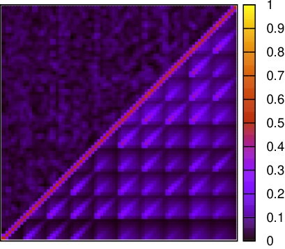
Figure 19: Comparison between the analytic correlation matrix (covariance normalized by the diagonals, i.e., $C_{ij}/\sqrt{C_{ii}C_{jj}}$) of four-bin tomographic cosmic shear power spectra and that derived from the HSC mock shear catalogs. The order of blocks is 11, 12, 13, 14, 22, 23, 24, 33, 34, 44 from left to right. We show the analytic correlation matrix in the lower right side of the triangle, whereas the absolute value of the difference between the analytic and mock correlation matrix is shown in the upper left side.

B.3 Comparison with mock catalogs

We compare the analytic covariance matrix with numerical estimates using HSC mock shear catalogs presented in Appendix A. We note that the HSC mock shear catalogs include cosmic shear from all-sky tracing simulations, and hence the covariance matrix computed from the mock catalogs naturally includes the effect of super-survey modes, which we also include in the analytic model. Figure 18 shows the comparison of the diagonal components of the covariance matrix of the tomographic cosmic shear power spectra. The diagonal components are dominated by the Gaussian term. Figure 19 compares the correlation coefficient matrices of tomographic cosmic shear power spectra. We find that our analytic model for the covariance well reproduces both the diagonal and off-diagonal parts of the covariance matrix derived numerically from the HSC shear mock catalogs. These comparisons demonstrate the validity of the use of the analytic model of the covariance matrix in our cosmological analysis.

Appendix C Convergence of our nested sampling results

The multimodal nested sampling algorithm called Multinest is a Bayesian inference tool to efficiently evaluate the Bayesian evidence as well as posterior distributions. The nested sampling performs Bayesian computations by maintaining a set of sample points (live points) in parameter space inside the prior $\pi(\theta)$ and repeatedly replacing the lowest likelihood point with another point with higher likelihood. The remaining fraction of the prior volume after the point with likelihood ${\cal L}_{i}$ is defined as

$$X({\cal L}_{i})\equiv\int_{{\cal L}(\theta)>{\cal L}_{i}}\pi(\theta)d\theta.$$ (77)

We note that $X$ exponentially shrinks as the likelihood ${\cal L}_{i}$ increases.

The nested sampling terminates when the remaining evidence contribution estimated as ${\cal L}_{\rm max}X_{i}$, where ${\cal L}_{\rm max}$ is the maximum likelihood value of the current set of live points and $X_{i}$ is the expected value of remaining prior volume, is less than a user-defined tolerance. We set the evidence tolerance factor tol=0.1, a value that is expected to be appropriate for the computation of Bayesian posterior and evidence. We set sampling efficiency ${\tt efr}=0.3$, which is the recommended value for evidence calculation (Feroz et al., 2009). We adopt importance nested sampling which obtains more accurate evidence values than does the standard nested sampling (Feroz et al., 2013), but we do not adopt the constant efficiency mode.

Another tuning parameter is the number of live points $N_{\rm live}$ at any given time. Larger $N_{\rm live}$ values increase the accuracy of the Bayesian evidence, although the computation cost also increases. Here we set $N_{\rm live}=2000$ to find that the standard deviations of $S_{8}$ and $\Omega_{\rm m}$ are $6.5\times 10^{-4}$ and $1.4\times 10^{-3}$ respectively estimated from 8 independent runs. These values are negligible compared to the marginalized 1$\sigma$ errors of these quantities (see Table 7). The standard deviation of the $\log X$ value is 0.041, which is also sufficiently small to enable the evaluation of the model preference from the evidence ratio.

The convergence of the nested sampling result can be demonstrated using the public diagnostic tool called nestcheck (Higson, 2018). Figure 20 is an output generated from nestcheck using the two nested sampling runs in the fiducial case. We show both the relative posterior mass at each $\log X$ value, i.e., ${\cal L}(X)X$, where ${\cal L}(X)\equiv X^{-1}({\cal L})$, and the distribution of $S_{8}$ at each $\log X$. The Figure demonstrates that our nested sampling run terminates at the point at which the relative posterior mass is very small and the $S_{8}$ value converges to the maximum likelihood point. The posterior distributions of the two nested sampling runs agree within the error estimated by bootstrap resampling.

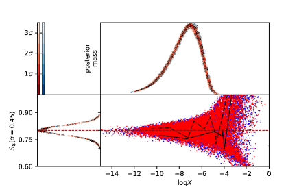
Figure 20: Distributions in $\log X$ produced using nestcheck for two nested sampling runs. The upper right panel shows the relative posterior mass at each $\log X$ value. The lower-right panel shows $S_{8}(\alpha=0.45)$ values against $\log X$ and the lower-left panels shows the posterior distributions. The solid black lines show the evolution of an individual thread from each run chosen at random. The colored contours show iso-probability credible intervals on the marginalized posterior probability density function. The figure indicates that our nested sampling runs terminate at the point at which the remaining fraction of posterior mass is sufficiently small.

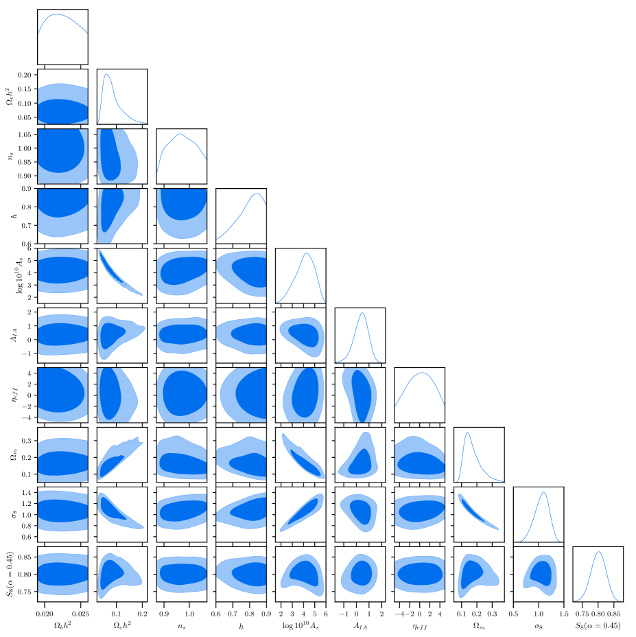
Figure 21: Marginalized one-dimensional and two-dimensional posteriors of cosmological model ($\Omega_{\rm b}h^{2}$, $\Omega_{\rm c}h^{2}$, $n_{s}$, $h$, $\log(10^{10}A_{s})$), and intrinsic alignment parameters ($A_{\rm IA}$, $\eta_{\rm eff}$) as well as derived parameters $\Omega_{\rm m}$, $\sigma_{8}$, and $S_{8}$ in the fiducial case. The contours in each two-dimensional constraint represent 68% and 95% credible intervals.

Appendix D Posterior distributions of the fiducial model parameters

Figure 21 shows the marginalized one-dimensional and two-dimensional posteriors of cosmological parameters and intrinsic alignment parameters as well as derived parameters $\Omega_{\rm m}$, $\sigma_{8}$, and $S_{8}$ in the fiducial setup. One can see that the posteriors for $\Omega_{\rm b}h^{2}$, $n_{s}$, and $h$ among 5 cosmological parameters are strongly affected by the prior as listed in Table 6. This is not surprising because the cosmic shear is not very sensitive to these parameters. For intrinsic alignment parameters, $\eta_{\rm eff}$ is prior-dominated whereas the amplitude parameter $A_{\rm IA}$ is well constrained from the data. We find that the prior of $h$ affects the quoted $\Omega_{\rm m}$ and $\sigma_{8}$ values, but probably does not affect the $S_{8}$ value since $h$ is not degenerate with $S_{8}$.

References

- Abbott et al. (2016) Abbott, T., Abdalla, F. B., Allam, S., et al. 2016, Phys. Rev. D, 94, 022001
- Aihara et al. (2018a) Aihara, H., Armstrong, R., Bickerton, S., et al. 2018a, PASJ, 70, S8
- Aihara et al. (2018b) Aihara, H., Arimoto, N., Armstrong, R., et al. 2018b, PASJ, 70, S4
- Alam et al. (2017) Alam, S., Ata, M., Bailey, S., et al. 2017, MNRAS, 470, 2617
- Albrecht et al. (2006) Albrecht, A., Bernstein, G., Cahn, R., et al. 2006, ArXiv Astrophysics e-prints, astro-ph/0609591
- Amendola et al. (2018) Amendola, L., Appleby, S., Avgoustidis, A., et al. 2018, Living Reviews in Relativity, 21, 2
- Anderson et al. (2014) Anderson, L., Aubourg, É., Bailey, S., et al. 2014, MNRAS, 441, 24
- Asgari et al. (2018) Asgari, M., Taylor, A., Joachimi, B., & Kitching, T. D. 2018, MNRAS, 479, 454
- Audren & Lesgourgues (2011) Audren, B., & Lesgourgues, J. 2011, JCAP, 10, 037
- Audren et al. (2013) Audren, B., Lesgourgues, J., Benabed, K., & Prunet, S. 2013, JCAP, 2, 001
- Bacon et al. (2003) Bacon, D. J., Massey, R. J., Refregier, A. R., & Ellis, R. S. 2003, MNRAS, 344, 673
- Bacon et al. (2000) Bacon, D. J., Refregier, A. R., & Ellis, R. S. 2000, MNRAS, 318, 625
- Bartelmann & Schneider (2001) Bartelmann, M., & Schneider, P. 2001, Phys. Rep., 340, 291
- Becker et al. (2016) Becker, M. R., Troxel, M. A., MacCrann, N., et al. 2016, Phys. Rev. D, 94, 022002
- Bernstein (2009) Bernstein, G. M. 2009, ApJ, 695, 652
- Bernstein & Jarvis (2002) Bernstein, G. M., & Jarvis, M. 2002, AJ, 123, 583
- Betoule et al. (2014) Betoule, M., Kessler, R., Guy, J., et al. 2014, A&A, 568, A22
- Beutler et al. (2011) Beutler, F., Blake, C., Colless, M., et al. 2011, MNRAS, 416, 3017
- Beutler et al. (2017) Beutler, F., Seo, H.-J., Saito, S., et al. 2017, MNRAS, 466, 2242
- Bird et al. (2012) Bird, S., Viel, M., & Haehnelt, M. G. 2012, MNRAS, 420, 2551
- Blake et al. (2011) Blake, C., Brough, S., Colless, M., et al. 2011, MNRAS, 415, 2876
- Blandford et al. (1991) Blandford, R. D., Saust, A. B., Brainerd, T. G., & Villumsen, J. V. 1991, MNRAS, 251, 600
- Blas et al. (2011) Blas, D., Lesgourgues, J., & Tram, T. 2011, JCAP, 7, 034
- Blazek et al. (2015) Blazek, J., Vlah, Z., & Seljak, U. 2015, JCAP, 8, 015
- Bonnett et al. (2016) Bonnett, C., Troxel, M. A., Hartley, W., et al. 2016, Phys. Rev. D, 94, 042005
- Bosch et al. (2018) Bosch, J., Armstrong, R., Bickerton, S., et al. 2018, PASJ, 70, S5
- Bridle & King (2007) Bridle, S., & King, L. 2007, New Journal of Physics, 9, 444
- Brown et al. (2005) Brown, M. L., Castro, P. G., & Taylor, A. N. 2005, MNRAS, 360, 1262
- Brown et al. (2003) Brown, M. L., Taylor, A. N., Bacon, D. J., et al. 2003, MNRAS, 341, 100
- Brown et al. (2002) Brown, M. L., Taylor, A. N., Hambly, N. C., & Dye, S. 2002, MNRAS, 333, 501
- Buchner et al. (2014) Buchner, J., Georgakakis, A., Nandra, K., et al. 2014, A&A, 564, A125
- Catelan et al. (2001) Catelan, P., Kamionkowski, M., & Blandford, R. D. 2001, MNRAS, 320, L7
- Chang et al. (2013) Chang, C., Jarvis, M., Jain, B., et al. 2013, MNRAS, 434, 2121
- Chang et al. (2019) Chang, C., Wang, M., Dodelson, S., et al. 2019, MNRAS, 482, 3696
- Chisari et al. (2018) Chisari, N. E., Richardson, M. L. A., Devriendt, J., et al. 2018, MNRAS, 480, 3962
- Cole et al. (2005) Cole, S., Percival, W. J., Peacock, J. A., et al. 2005, MNRAS, 362, 505
- Cooray & Hu (2001) Cooray, A., & Hu, W. 2001, ApJ, 554, 56
- Cooray & Sheth (2002) Cooray, A., & Sheth, R. 2002, Phys. Rep., 372, 1
- Croft & Metzler (2000) Croft, R. A. C., & Metzler, C. A. 2000, ApJ, 545, 561
- DES Collaboration et al. (2017) DES Collaboration, Abbott, T. M. C., Abdalla, F. B., et al. 2017, arXiv e-prints, arXiv:1708.01530
- Diemer (2018) Diemer, B. 2018, ApJS, 239, 35
- Diemer & Kravtsov (2015) Diemer, B., & Kravtsov, A. V. 2015, ApJ, 799, 108
- Efstathiou & Lemos (2018) Efstathiou, G., & Lemos, P. 2018, MNRAS, 476, 151
- Feroz & Hobson (2008) Feroz, F., & Hobson, M. P. 2008, MNRAS, 384, 449
- Feroz et al. (2009) Feroz, F., Hobson, M. P., & Bridges, M. 2009, MNRAS, 398, 1601
- Feroz et al. (2013) Feroz, F., Hobson, M. P., Cameron, E., & Pettitt, A. N. 2013, ArXiv e-prints, arXiv:1306.2144
- Friedrich et al. (2016) Friedrich, O., Seitz, S., Eifler, T. F., & Gruen, D. 2016, MNRAS, 456, 2662
- Furusawa et al. (2018) Furusawa, H., Koike, M., Takata, T., et al. 2018, PASJ, 70, S3
- Gruen & Brimioulle (2017) Gruen, D., & Brimioulle, F. 2017, MNRAS, 468, 769
- Hamana et al. (2003) Hamana, T., Miyazaki, S., Shimasaku, K., et al. 2003, ApJ, 597, 98
- Harnois-Déraps et al. (2015) Harnois-Déraps, J., van Waerbeke, L., Viola, M., & Heymans, C. 2015, MNRAS, 450, 1212
- Hartlap et al. (2007) Hartlap, J., Simon, P., & Schneider, P. 2007, A&A, 464, 399
- Heavens et al. (2000) Heavens, A., Refregier, A., & Heymans, C. 2000, MNRAS, 319, 649
- Hellwing et al. (2016) Hellwing, W. A., Schaller, M., Frenk, C. S., et al. 2016, MNRAS, 461, L11
- Heymans et al. (2012) Heymans, C., Van Waerbeke, L., Miller, L., et al. 2012, MNRAS, 427, 146
- Heymans et al. (2013) Heymans, C., Grocutt, E., Heavens, A., et al. 2013, MNRAS, 432, 2433
- Higson (2018) Higson, E. 2018, The Journal of Open Source Software, 3, 916
- Hikage & Oguri (2016) Hikage, C., & Oguri, M. 2016, MNRAS, 462, 1359
- Hikage et al. (2011) Hikage, C., Takada, M., Hamana, T., & Spergel, D. 2011, MNRAS, 412, 65
- Hildebrandt et al. (2017) Hildebrandt, H., Viola, M., Heymans, C., et al. 2017, MNRAS, 465, 1454
- Hinshaw et al. (2013) Hinshaw, G., Larson, D., Komatsu, E., et al. 2013, ApJS, 208, 19
- Hirata & Seljak (2003) Hirata, C., & Seljak, U. 2003, MNRAS, 343, 459
- Hirata & Seljak (2004) Hirata, C. M., & Seljak, U. 2004, Phys. Rev. D, 70, 063526
- Hivon et al. (2002) Hivon, E., Górski, K. M., Netterfield, C. B., et al. 2002, ApJ, 567, 2
- Hoekstra et al. (2002) Hoekstra, H., Yee, H. K. C., & Gladders, M. D. 2002, ApJ, 577, 595
- Hogg et al. (2004) Hogg, D. W., Blanton, M. R., Brinchmann, J., et al. 2004, ApJ, 601, L29
- Hoyle et al. (2018) Hoyle, B., Gruen, D., Bernstein, G. M., et al. 2018, MNRAS, 478, 592
- Hsieh & Yee (2014) Hsieh, B. C., & Yee, H. K. C. 2014, ApJ, 792, 102
- Hu (1999) Hu, W. 1999, ApJ, 522, L21
- Huang et al. (2018) Huang, S., Leauthaud, A., Murata, R., et al. 2018, PASJ, 70, S6
- Huterer & Takada (2005) Huterer, D., & Takada, M. 2005, Astroparticle Physics, 23, 369
- Ilbert et al. (2009) Ilbert, O., Capak, P., Salvato, M., et al. 2009, ApJ, 690, 1236
- Iršič et al. (2017) Iršič, V., Viel, M., Berg, T. A. M., et al. 2017, MNRAS, 466, 4332
- Jarvis et al. (2003) Jarvis, M., Bernstein, G. M., Fischer, P., et al. 2003, AJ, 125, 1014
- Jarvis et al. (2016) Jarvis, M., Sheldon, E., Zuntz, J., et al. 2016, MNRAS, 460, 2245
- Jee et al. (2016) Jee, M. J., Tyson, J. A., Hilbert, S., et al. 2016, ApJ, 824, 77
- Jing et al. (2006) Jing, Y. P., Zhang, P., Lin, W. P., Gao, L., & Springel, V. 2006, ApJ, 640, L119
- Joachimi et al. (2011) Joachimi, B., Mandelbaum, R., Abdalla, F. B., & Bridle, S. L. 2011, A&A, 527, A26
- Joachimi et al. (2015) Joachimi, B., Cacciato, M., Kitching, T. D., et al. 2015, Space Sci. Rev., 193, 1
- Joudaki et al. (2017a) Joudaki, S., Blake, C., Heymans, C., et al. 2017a, MNRAS, 465, 2033
- Joudaki et al. (2017b) Joudaki, S., Mead, A., Blake, C., et al. 2017b, MNRAS, 471, 1259
- Joudaki et al. (2018) Joudaki, S., Blake, C., Johnson, A., et al. 2018, MNRAS, 474, 4894
- Kaiser (1992) Kaiser, N. 1992, ApJ, 388, 272
- Kaiser et al. (1995) Kaiser, N., Squires, G., & Broadhurst, T. 1995, ApJ, 449, 460
- Kaiser et al. (2000) Kaiser, N., Wilson, G., & Luppino, G. A. 2000, ArXiv Astrophysics e-prints, astro-ph/0003338
- Kawanomoto et al. (2018) Kawanomoto, S., Uraguchi, F., Komiyama, Y., et al. 2018, PASJ, 70, 66
- Kiessling et al. (2015) Kiessling, A., Cacciato, M., Joachimi, B., et al. 2015, Space Sci. Rev., 193, 67
- Kilbinger (2015) Kilbinger, M. 2015, Reports on Progress in Physics, 78, 086901
- Kilbinger et al. (2013) Kilbinger, M., Fu, L., Heymans, C., et al. 2013, MNRAS, 430, 2200
- Kilbinger et al. (2017) Kilbinger, M., Heymans, C., Asgari, M., et al. 2017, MNRAS, 472, 2126
- Kirk et al. (2015) Kirk, D., Brown, M. L., Hoekstra, H., et al. 2015, Space Sci. Rev., 193, 139
- Kitching et al. (2017) Kitching, T. D., Alsing, J., Heavens, A. F., et al. 2017, MNRAS, 469, 2737
- Kitching et al. (2012) Kitching, T. D., Balan, S. T., Bridle, S., et al. 2012, MNRAS, 423, 3163
- Kitching et al. (2014) Kitching, T. D., Heavens, A. F., Alsing, J., et al. 2014, MNRAS, 442, 1326
- Kogut et al. (2003) Kogut, A., Spergel, D. N., Barnes, C., et al. 2003, ApJS, 148, 161
- Köhlinger et al. (2018) Köhlinger, F., Joachimi, B., Asgari, M., et al. 2018, ArXiv e-prints, arXiv:1809.01406
- Köhlinger et al. (2017) Köhlinger, F., Viola, M., Joachimi, B., et al. 2017, MNRAS, 471, 4412
- Komiyama et al. (2018) Komiyama, Y., Obuchi, Y., Nakaya, H., et al. 2018, PASJ, 70, S2
- Kuijken et al. (2015) Kuijken, K., Heymans, C., Hildebrandt, H., et al. 2015, MNRAS, 454, 3500
- Laigle et al. (2016) Laigle, C., McCracken, H. J., Ilbert, O., et al. 2016, ApJS, 224, 24
- Laureijs et al. (2011) Laureijs, R., Amiaux, J., Arduini, S., et al. 2011, ArXiv e-prints, arXiv:1110.3193
- Le Fèvre et al. (2013) Le Fèvre, O., Cassata, P., Cucciati, O., et al. 2013, A&A, 559, A14
- Leauthaud et al. (2007) Leauthaud, A., Massey, R., Kneib, J.-P., et al. 2007, ApJS, 172, 219
- Lee & Pen (2000) Lee, J., & Pen, U.-L. 2000, ApJ, 532, L5
- Lesgourgues (2011) Lesgourgues, J. 2011, ArXiv e-prints, arXiv:1104.2932
- Lesgourgues et al. (2013) Lesgourgues, J., Mangano, G., Miele, G., & Pastor, S. 2013, Neutrino Cosmology
- Lewis & Bridle (2002) Lewis, A., & Bridle, S. 2002, Phys. Rev. D, 66, 103511
- Li et al. (2014) Li, Y., Hu, W., & Takada, M. 2014, Phys. Rev. D, 89, 083519
- Lima et al. (2008) Lima, M., Cunha, C. E., Oyaizu, H., et al. 2008, MNRAS, 390, 118
- Liske et al. (2015) Liske, J., Baldry, I. K., Driver, S. P., et al. 2015, MNRAS, 452, 2087
- LSST Science Collaboration et al. (2009) LSST Science Collaboration, Abell, P. A., Allison, J., et al. 2009, ArXiv e-prints, arXiv:0912.0201
- Mandelbaum (2018) Mandelbaum, R. 2018, Ann. Rev. Astron. Astrophys., 56, 393
- Mandelbaum et al. (2013) Mandelbaum, R., Slosar, A., Baldauf, T., et al. 2013, MNRAS, 432, 1544
- Mandelbaum et al. (2005) Mandelbaum, R., Hirata, C. M., Seljak, U., et al. 2005, MNRAS, 361, 1287
- Mandelbaum et al. (2018a) Mandelbaum, R., Miyatake, H., Hamana, T., et al. 2018a, PASJ, 70, S25
- Mandelbaum et al. (2018b) Mandelbaum, R., Lanusse, F., Leauthaud, A., et al. 2018b, MNRAS, 481, 3170
- Maoli et al. (2001) Maoli, R., Van Waerbeke, L., Mellier, Y., et al. 2001, A&A, 368, 766
- Marshall et al. (2006) Marshall, P., Rajguru, N., & Slosar, A. 2006, Phys. Rev. D, 73, 067302
- Masters et al. (2015) Masters, D., Capak, P., Stern, D., et al. 2015, ApJ, 813, 53
- McCarthy et al. (2018) McCarthy, I. G., Bird, S., Schaye, J., et al. 2018, MNRAS, 476, 2999
- McCarthy et al. (2017) McCarthy, I. G., Schaye, J., Bird, S., & Le Brun, A. M. C. 2017, MNRAS, 465, 2936
- McDonald et al. (2006) McDonald, P., Seljak, U., Burles, S., et al. 2006, ApJS, 163, 80
- McQuinn & White (2013) McQuinn, M., & White, M. 2013, MNRAS, 433, 2857
- Mead et al. (2015) Mead, A. J., Peacock, J. A., Heymans, C., Joudaki, S., & Heavens, A. F. 2015, MNRAS, 454, 1958
- Ménard et al. (2013) Ménard, B., Scranton, R., Schmidt, S., et al. 2013, ArXiv e-prints, arXiv:1303.4722
- Miralda-Escude (1991) Miralda-Escude, J. 1991, ApJ, 380, 1
- Miyazaki et al. (2012) Miyazaki, S., Komiyama, Y., Nakaya, H., et al. 2012, in Proc. SPIE, Vol. 8446, Ground-based and Airborne Instrumentation for Astronomy IV, 84460Z
- Miyazaki et al. (2015) Miyazaki, S., Oguri, M., Hamana, T., et al. 2015, ApJ, 807, 22
- Miyazaki et al. (2018) Miyazaki, S., Komiyama, Y., Kawanomoto, S., et al. 2018, PASJ, 70, S1
- Murata et al. (2018) Murata, R., Nishimichi, T., Takada, M., et al. 2018, ApJ, 854, 120
- Navarro et al. (1997) Navarro, J. F., Frenk, C. S., & White, S. D. M. 1997, ApJ, 490, 493
- Newman (2008) Newman, J. A. 2008, ApJ, 684, 88
- Norberg et al. (2009) Norberg, P., Baugh, C. M., Gaztañaga, E., & Croton, D. J. 2009, MNRAS, 396, 19
- Oguri et al. (2018) Oguri, M., Miyazaki, S., Hikage, C., et al. 2018, PASJ, 70, S26
- Oka et al. (2014) Oka, A., Saito, S., Nishimichi, T., Taruya, A., & Yamamoto, K. 2014, MNRAS, 439, 2515
- Osato et al. (2015) Osato, K., Shirasaki, M., & Yoshida, N. 2015, ApJ, 806, 186
- Padmanabhan et al. (2005) Padmanabhan, N., Budavári, T., Schlegel, D. J., et al. 2005, MNRAS, 359, 237
- Palanque-Delabrouille et al. (2013) Palanque-Delabrouille, N., Yèche, C., Borde, A., et al. 2013, A&A, 559, A85
- Percival et al. (2002) Percival, W. J., Sutherland, W., Peacock, J. A., et al. 2002, MNRAS, 337, 1068
- Percival et al. (2010) Percival, W. J., Reid, B. A., Eisenstein, D. J., et al. 2010, MNRAS, 401, 2148
- Planck Collaboration et al. (2016) Planck Collaboration, Ade, P. A. R., Aghanim, N., et al. 2016, A&A, 594, A13
- Planck Collaboration et al. (2018) Planck Collaboration, Aghanim, N., Akrami, Y., et al. 2018, ArXiv e-prints, arXiv:1807.06209
- Raveri & Hu (2018) Raveri, M., & Hu, W. 2018, ArXiv e-prints, arXiv:1806.04649
- Reid et al. (2010) Reid, B. A., Percival, W. J., Eisenstein, D. J., et al. 2010, MNRAS, 404, 60
- Rhodes et al. (2001) Rhodes, J., Refregier, A., & Groth, E. J. 2001, ApJ, 552, L85
- Riess et al. (2018) Riess, A. G., Casertano, S., Yuan, W., et al. 2018, ApJ, 855, 136
- Ross et al. (2015) Ross, A. J., Samushia, L., Howlett, C., et al. 2015, MNRAS, 449, 835
- Sato et al. (2009) Sato, M., Hamana, T., Takahashi, R., et al. 2009, ApJ, 701, 945
- Schaye et al. (2010) Schaye, J., Dalla Vecchia, C., Booth, C. M., et al. 2010, MNRAS, 402, 1536
- Schneider et al. (2013) Schneider, M. D., Cole, S., Frenk, C. S., et al. 2013, MNRAS, 433, 2727
- Scoccimarro et al. (1999) Scoccimarro, R., Zaldarriaga, M., & Hui, L. 1999, ApJ, 527, 1
- Semboloni et al. (2011) Semboloni, E., Hoekstra, H., Schaye, J., van Daalen, M. P., & McCarthy, I. G. 2011, MNRAS, 417, 2020
- Sifón et al. (2015) Sifón, C., Hoekstra, H., Cacciato, M., et al. 2015, A&A, 575, A48
- Simon et al. (2004) Simon, P., King, L. J., & Schneider, P. 2004, A&A, 417, 873
- Singh et al. (2015) Singh, S., Mandelbaum, R., & More, S. 2015, MNRAS, 450, 2195
- Smith et al. (2003) Smith, R. E., Peacock, J. A., Jenkins, A., et al. 2003, MNRAS, 341, 1311
- Spergel et al. (2015) Spergel, D., Gehrels, N., Baltay, C., et al. 2015, ArXiv e-prints, arXiv:1503.03757
- Springel et al. (2018) Springel, V., Pakmor, R., Pillepich, A., et al. 2018, MNRAS, 475, 676
- Suzuki et al. (2012) Suzuki, N., Rubin, D., Lidman, C., et al. 2012, ApJ, 746, 85
- Takada & Bridle (2007) Takada, M., & Bridle, S. 2007, New Journal of Physics, 9, 446
- Takada & Hu (2013) Takada, M., & Hu, W. 2013, Phys. Rev. D, 87, 123504
- Takada & Jain (2003) Takada, M., & Jain, B. 2003, MNRAS, 344, 857
- Takada & Jain (2004) —. 2004, MNRAS, 348, 897
- Takada & Jain (2009) —. 2009, MNRAS, 395, 2065
- Takada et al. (2006) Takada, M., Komatsu, E., & Futamase, T. 2006, Phys. Rev. D, 73, 083520
- Takahashi et al. (2017) Takahashi, R., Hamana, T., Shirasaki, M., et al. 2017, ApJ, 850, 24
- Takahashi et al. (2012) Takahashi, R., Sato, M., Nishimichi, T., Taruya, A., & Oguri, M. 2012, ApJ, 761, 152
- Tanaka (2015) Tanaka, M. 2015, ApJ, 801, 20
- Tanaka et al. (2018) Tanaka, M., Coupon, J., Hsieh, B.-C., et al. 2018, PASJ, 70, S9
- Tegmark et al. (2004) Tegmark, M., Strauss, M. A., Blanton, M. R., et al. 2004, Phys. Rev. D, 69, 103501
- Tinker et al. (2008) Tinker, J., Kravtsov, A. V., Klypin, A., et al. 2008, ApJ, 688, 709
- Tinker et al. (2010) Tinker, J. L., Robertson, B. E., Kravtsov, A. V., et al. 2010, ApJ, 724, 878
- Troxel et al. (2018a) Troxel, M. A., MacCrann, N., Zuntz, J., et al. 2018a, Phys. Rev. D, 98, 043528
- Troxel et al. (2018b) Troxel, M. A., Krause, E., Chang, C., et al. 2018b, MNRAS, 479, 4998
- van Daalen et al. (2011) van Daalen, M. P., Schaye, J., Booth, C. M., & Dalla Vecchia, C. 2011, MNRAS, 415, 3649
- van Uitert et al. (2018) van Uitert, E., Joachimi, B., Joudaki, S., et al. 2018, MNRAS, 476, 4662
- Van Waerbeke et al. (2000) Van Waerbeke, L., Mellier, Y., Erben, T., et al. 2000, A&A, 358, 30
- Van Waerbeke et al. (2001) Van Waerbeke, L., Mellier, Y., Radovich, M., et al. 2001, A&A, 374, 757
- Viel et al. (2013) Viel, M., Becker, G. D., Bolton, J. S., & Haehnelt, M. G. 2013, Phys. Rev. D, 88, 043502
- Vogelsberger et al. (2014) Vogelsberger, M., Genel, S., Springel, V., et al. 2014, Nature, 509, 177
- White (2004) White, M. 2004, Astroparticle Physics, 22, 211
- Wittman et al. (2000) Wittman, D. M., Tyson, J. A., Kirkman, D., Dell’Antonio, I., & Bernstein, G. 2000, Nature, 405, 143
- Yamamoto et al. (2006) Yamamoto, K., Nakamichi, M., Kamino, A., Bassett, B. A., & Nishioka, H. 2006, PASJ, 58, 93
- Yoon et al. (2018) Yoon, M., Jee, M. J., Tyson, J. A., et al. 2018, ArXiv e-prints, arXiv:1807.09195
- Zhan & Knox (2004) Zhan, H., & Knox, L. 2004, ApJ, 616, L75