Handling Handles. Part II.
Stratification and Data Analysis

1 Introduction

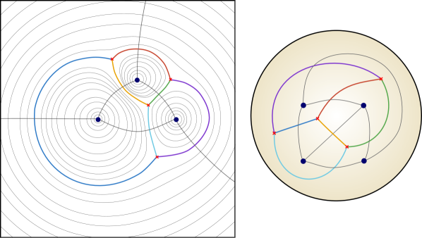
Figure 1: In the left figure, four strings radiated from four worldsheet punctures interact (blue dots, with the fourth puncture located at infinity). The punctures are encircled by contour lines of constant worldsheet time (black). Critical lines (colorful) divide the contour lines encircling different punctures. The critical lines intersect at the red crosses, and thus define a cubic graph. The dual graph is shown in gray. On the right, we represent a standard tree-level field-theory four-point graph with the topology of a sphere (gray), as well as its dual graph (colorful).

Like in any perturbative string theory, closed string amplitudes in $\mathrm{AdS}_{5}\times\mathrm{S}^{5}$ superstring theory are given by integrations over the moduli space of Riemann surfaces of various genus. Like in any large-$N_{\text{c}}$ gauge theory, correlation functions of local single-trace gauge-invariant operators in $\mathcal{N}=4$ SYM theory are given by sums over double-line Feynman (ribbon) graphs of various genus. By virtue of the AdS/CFT duality, these two quantities ought to be the same. Clearly, to better understand the nature of holography, it is crucial to understand how the sum over graphs connects to the integration over the string moduli.

Our proposal in [1] provides one realization. It can be motivated as a finite-coupling extension of a very nice proposal by Razamat [2], built up on the works of Gopakumar et al. [3, 4, 5, 6, 7, 8], which in turn relied on beautiful classical mathematics by Strebel [9, 10], where an isomorphism between the space of metric ribbon graphs and moduli spaces of Riemann surfaces was first understood.

Let us briefly describe some of these ideas. Figure 1 is a very inspiring example, so let us explain a few of its features. The figure describes four strings interacting at tree level, i. e. a four-punctured sphere (in the figure, one of the punctures is at infinity). The black lines are sections of the incoming strings. Close to each puncture, the string world-sheet behaves as a normal single string, so here the black lines are simple circles. They are the lines of constant $\tau$ for each string. These lines of constant $\tau$ need to fit together into a global picture, as shown in the figure. Note that there are four special points, the red crosses, which can be connected along critical lines (the colorful lines), across which we “jump from one string to another”. These critical lines define a graph. There is also a dual graph, drawn in gray. This construction creates a map between the moduli space of a four-punctured Riemann sphere and a class of graphs, as anticipated above.

These cartoons can be made mathematically rigorous. For each punctured Riemann surface, there is a unique quadratic differential $\phi$, called the Strebel differential, with fixed residues at each puncture, which decomposes the surface into disk-like regions – the faces delimited by the colorful lines [9, 10] (see the appendices in [2] for a beautiful review). The red crosses are the zeros of the Strebel differential. The line integrals between these critical points, i. e. the integrals along the colorful lines are real, and thus define a (positive) length for each line of the graph. In this way the graph becomes a metric graph. (The sum over the lengths of the critical lines that encircle a puncture equals the residue of the Strebel differential at that puncture by contour integral arguments.) By construction, the critical lines emanating from each zero have a definite ordering around that zero. This ordering can equivalently be achieved by promoting each line to a “ribbon” by giving it a non-zero width; for this reason the relevant graphs are called metric ribbon graphs. Conversely, fixing a graph topology and assigning a length to each edge uniquely fixes the Strebel differential and thus a point in the moduli space.

Such metric ribbon graphs, like the one on the right of Figure 1, also arise at zero coupling in the dual gauge theory. There, the number associated to each line is nothing but the number of propagators connecting two operators along that line. These numbers are thus integers in this case, as emphasized in [2]. Note that the total number of lines getting out of a given operator is fixed, which is the gauge-theory counterpart of the above contour integral argument.

As such, it is very tempting to propose that we fix the residue of the Strebel differential at each puncture to be equal to the number of fields inside the trace of the dual operator. Then there is a discrete subset of points within the string moduli space where those integer residues are split into integer subsets, which define a valid gauge-theory ribbon graph. By our weak-coupling analysis, it seems that the string path integral is localizing at these points. Note that the graphs defined by the Strebel differential change as we move in the string moduli space, and that all free gauge-theory graphs nicely show up when doing so, such that the map is truly complete. The jump from one graph to another is mathematically very similar to the wall-crossing phenomenon within the space of $4$d $\mathcal{N}=2$ theories [25, 26].

What about finite coupling? Here it is where the hexagons come in. The gray lines in Figure 1 typically define a triangulation of the Riemann surface (since the colored dual graph is a cubic graph). The triangular faces become hexagons once we blow up all punctures into small circles, such that small extra segments get inserted into all triangle vertices, effectively converting all triangles into hexagons. In order to glue together these hexagons, we insert a complete basis of (open mirror) string states at each of the gray lines. The sum over these complete bases of states can be thought of as exploring the vicinity of each discrete point in the moduli space, thus covering the full string path integral.

For correlation functions of more/fewer operators, and/or different worldsheet genus, the picture is very similar. What changes, of course, is the number of zeros of the Strebel differential, that is the number of hexagon operators we should glue together. In the example above, we had four red crosses, that is four hexagons. This number is very easy to understand. Topologically, a four-point function can be thought of as gluing together two pairs of pants, and each pair of pants is the union of two hexagons. To obtain a genus $g$ correlation function of $n$ closed strings, we would glue together $2n+4g-4$ hexagons. We ought to glue all these hexagons together and sum over a complete basis of mirror states on each gluing line. Each hexagon has three such mirror lines, as illustrated in Figure 1, and each line is shared by two hexagons, so there will be a $(3n+6g-6)$-fold sum over mirror states. This is admissibly a hard task, but, until now, there is no alternative for studying correlation functions at finite coupling and genus in this gauge theory. So this is the best we have thus far.

For higher genus – i. e. as we venture into the non-planar regime – there is a final and very important ingredient called the stratification, which appeared already in the context of matrix models [29, 30, 31], and which gives the name to this paper. It can be motivated from gauge theory as well as from string theory considerations. From the gauge theory viewpoint, it is clear that simply drawing all tree-level graphs of a given genus, and dressing them by hexagons and mirror states cannot be the full story: As we go to higher loops in ’t Hooft coupling, there will be handles formed by purely virtual processes, which are not present at lower orders. So including only genus-$g$ tree-level graphs misses some contributions. One naive idea would be to include – at a given genus – all graphs which can be drawn on surfaces of that genus or less. But this would be no good either, as it would vastly over-count contributions. The stratification procedure explained in this paper prescribes precisely which contributions have to be added or subtracted, so that – we hope – everything works out. From a string theory perspective, this stratification originates in the boundaries of the moduli space. We can have tori, for example, degenerating into spheres, and to properly avoid missing (or double-counting) such degenerate contributions, we need to carefully understand what to sum over. In more conventional string perturbation theory, we are used to continuous integrations over the moduli space, where such degenerate contributions typically amount to measure-zero sets, which we can ignore. But here – as emphasized above and already proposed in [2] – the sum is rather a discrete one, hence missing or adding particular terms matters.

All in all, our final proposal can be summarized in equation (LABEL:eq:mainformula) below, where the seemingly innocuous $\mathcal{S}$ operation is the stratification procedure, which is further motivated and made precise below, see e. g. (2.24) for a taste of what it ends up looking like.

In the end, all this is a plausible yet conjectural picture. Clearly, many checks are crucial to validate this proposal, and to iron out its details. A most obvious test is to carry out the hexagonalization and stratification procedure to study the first non-planar quantum correction to a gauge-theory four-point correlation function, and to compare the result with available perturbative data. That is what this paper is about.

2 Developing the Proposal

In the following, we introduce our main formula and explain its ingredients in Section 2.1. In the subsequent Section 2.2, we explain the summation over graphs at the example of a four-point function on the torus. Section 2.3 and Section 2.4 are devoted to the effects of stratification.

2.1 The Main Formula

Recall that in a general large-$N_{\text{c}}$ gauge theory with adjoint matter, each Feynman diagram is assigned a genus by promoting all propagators to double-lines (pairs of fundamental color lines). At each single-trace operator insertion, the color trace induces a definite ordering of the attached (double) lines. By this ordering, the color lines of the resulting double-line graph form well-defined closed loops. Assigning an oriented disk (face) to each of these color loops, we obtain an oriented compact surface. The genus of the graph (Wick contraction) is the genus of this surface. Counting powers of $N_{\text{c}}$ and $g_{\scriptscriptstyle\mathrm{YM}}^{2}$ for propagators (${\sim}g_{\scriptscriptstyle\mathrm{YM}}^{2}$), vertices (${\sim}1/g_{\scriptscriptstyle\mathrm{YM}}^{2}$), and faces (${\sim}N_{\text{c}}$), taking into account that every operator insertion adds a boundary component to the surface, absorbing one power of $N_{\text{c}}$ into the ’t Hooft coupling $\lambda=g_{\scriptscriptstyle\mathrm{YM}}^{2}N_{\text{c}}$, and using the formula for the Euler characteristic, we arrive at the well-known genus expansion formula [32] for connected correlators of (canonically normalized) single-trace operators $\mathcal{O}_{i}$:

$$\langle\mathcal{O}_{1}\dotsc\mathcal{O}_{n}\rangle=\frac{1}{N_{\text{c}}^{n-2}}\sum_{g=0}^{\infty}\frac{1}{N_{\text{c}}^{2g}}\,\mathcal{G}_{1,\dotsc,n}^{(g)}(\lambda)\,,\qquad\lambda=g_{\scriptscriptstyle\mathrm{YM}}^{2}N_{\text{c}}\,.$$ (2.1)

Here, $\mathcal{G}_{1,\dotsc,n}^{(g)}(\lambda)$ is the correlator restricted to genus-$g$ contributions. Via the AdS/CFT duality, the surface defined by Feynman diagrams at large $N_{\text{c}}$ becomes the worldsheet of the dual string with $n$ vertex operator insertions.

The purpose of this paper is to give a concrete and explicit realization of the general large-$N_{\text{c}}$ genus expansion formula (2.1) for the case of $\mathcal{N}=4$ super Yang–Mills theory. The proposed formula is based on the integrability of the (gauge/worldsheet/string) theory, and should be valid at any order in the ’t Hooft coupling constant $\lambda$. The general formula reads Let us explain the ingredients: The operators $\mathcal{Q}_{i}$ we consider are half-BPS operators, which are characterized by a position $x_{i}$, an internal polarization $\alpha_{i}$, and a weight $k_{i}$,

$$\mathcal{Q}_{i}=\mathcal{Q}(\alpha_{i},x_{i},k_{i})=\operatorname{tr}\left((\alpha_{i}\cdot\Phi(x_{i}))^{k_{i}}\right)\,,\qquad\alpha_{i}^{2}=0\,.$$ (2.2)

Here, $\Phi=(\Phi_{1},\dotsc,\Phi_{6})$ are the six real scalar fields of $\mathcal{N}=4$ super Yang–Mills theory, and $\alpha$ is a six-dimensional null vector. We start with the set $\mathbold{\Gamma}$ of all Wick contractions of the $n$ operators in the free theory. Each Wick contraction defines a graph, whose edges are the propagators. We will use the terms “graph” and “Wick contraction” interchangeably. By the procedure described above, we can associate a compact oriented surface to each Wick contraction, and thereby define the genus $g(\Gamma)$ of any given graph $\Gamma$. Importantly, the edges emanating from each operator have a definite ordering around that operator due to the color trace in (2.2).

Next, we promote each graph $\Gamma$ to a triangulation $\Gamma_{\triangle}$ in two steps: First, we identify (“glue together”) all homotopically equivalent (that is, parallel and non-crossing) lines of the original graph $\Gamma$. The resulting graph is called a skeleton graph. We can assign a “width” to each line of the skeleton graph, which equals the number of lines (propagators) that have been identified. Each line of the skeleton graph is called a bridge $b$, and the width of the line is conventionally called the bridge length $\ell_{b}$. There is a propagator factor $d_{b}^{\ell_{b}}$ for each bridge. By definition, each face of a skeleton graph is bounded by three or more bridges. In a second step, we subdivide faces that are bounded by $(m>3)$ bridges into triangles by inserting $(m-3)$ further zero-length bridges (ZLBs). Using the formula for the Euler characteristic, one finds that the fully triangulated graph $\Gamma_{\triangle}$ has $2n+4g(\Gamma)-4$ faces.

For each bridge $b$ of the triangulated skeleton graph $\Gamma_{\triangle}$, we integrate over a complete set of states $\psi_{b}$ living on that bridge, and we insert a weight factor $\mathcal{W}(\psi_{b})$. The weight factor measures the charges of the state $\psi_{b}$ under a superconformal transformation that relates the two adjacent triangular faces; it thus depends on both the cross ratios of the four neighboring vertices, and on the labels of the state $\psi_{b}$. The worldsheet theory on each bridge is a “mirror theory” which is obtained from the physical worldsheet theory by an analytic continuation via a double-Wick rotation. States in this theory are composed of magnons with definite rapidities $u_{i}\in\mathbb{R}$ and bound state indices $a_{i}\in\mathbb{Z}_{\geq 1}$. A complete set of states is given by all Bethe states, where each Bethe state is characterized by the number $m$ of magnons, their rapidities $\{u_{1},\dotsc,u_{m}\}$, their bound state indices $\{a_{1},\dotsc,a_{m}\}$, and their $\mathfrak{su}(2|2)^{2}$ flavor labels $(A,\dot{A})$. The integration over the space $\mathbold{M}_{b}$ of mirror states hence expands to

$$\int_{\mathbold{M}_{b}}\mathrm{d}\psi_{b}=\sum_{m=0}^{\infty}\prod_{i=1}^{m}\sum_{a_{i}=1}^{\infty}\sum_{A_{i},\dot{A}_{i}}\int_{u_{i}=-\infty}^{\infty}\mathrm{d}u_{i}\,\mu_{a_{i}}(u_{i})\,e^{-\tilde{E}_{a_{i}}(u_{i})\,\ell_{b}}\,,$$ (2.3)

where $\mu_{a_{i}}(u_{i})$ is a measure factor, $\tilde{E}$ is the mirror energy, $\ell_{b}$ is the length of the bridge $b$, and the exponential is a Boltzmann factor for the propagation of the mirror particles across the bridge.

Finally, each face $a$ of the triangulated skeleton graph $\Gamma_{\triangle}$ carries one hexagon form factor $\mathcal{H}_{a}$, which accounts for the interactions among the three physical operators $\mathcal{Q}_{i}$, $\mathcal{Q}_{j}$, $\mathcal{Q}_{k}$ as well as the mirror states on the three edges $b_{1}$, $b_{2}$, $b_{3}$ adjacent to the face. It is therefore a function of all this data:

$$\mathcal{H}_{a}=\mathcal{H}_{a}(x_{i},\alpha_{i},x_{j},\alpha_{j},x_{k},\alpha_{k};\psi_{b_{1}},\psi_{b_{2}},\psi_{b_{3}})\,.$$ (2.4)

The hexagon form factor is a worldsheet branch-point twist operator that inserts an excess angle of $\pi$ on the worldsheet. It has been introduced in [15] for the purpose of computing planar three-point functions, and has later been applied to compute planar four-point [11, 12] and five-point functions [14]. Our formula (LABEL:eq:mainformula) is an extension and generalization of these works to the non-planar regime. Notably, all ingredients of the formula (LABEL:eq:mainformula) (measures $\mu_{a}(u)$, mirror energies $\tilde{E}_{a}(u)$, and hexagon form factors $\mathcal{H}$) are known as exact functions of the coupling $\lambda$, and hence the formula should be valid at finite coupling. The hexagon form factors are given in terms of the Beisert S-matrix [35], the dressing phase [36], as well as analytic continuations among the three physical and the three mirror theories on the perimeter of the hexagon [15].

Unlike the general genus expansion (2.1), the formula (LABEL:eq:mainformula) nicely separates the combinatorial sum over graphs and topologies from the coupling dependence, since the sum over graphs only runs over Wick contractions of the free theory. At any fixed genus, the list of contributing graphs can be constructed once and for all. The dependence on the coupling $\lambda$ sits purely in the dynamics of the integrable hexagonal patches of worldsheet $\mathcal{H}$ and their gluing properties.

Finally, we have the very important stratification operation indicated by the operator ${\mathcal{S}}$ in (LABEL:eq:mainformula). The basic idea already anticipated in the introduction is that the sum over graphs mimics the integration over the string moduli space, which contains boundaries. At those boundaries, it is crucial to avoid missing or over-counting contributions, specially in a discrete sum as we have here. Despite its innocuous appearance, it is perhaps the most non-trivial aspect of this paper and is discussed in great detail below; the curious reader can give a quick peek at (2.24) below.

In the remainder of this paper, we will flesh out the details of the formula (LABEL:eq:mainformula), test it against known perturbative data at genus one, and use it to make a few higher-loop predictions.

2.2 Polygonization and Hexagonalization

The combinatorial part of the prescription is to sum over planar contractions of $n$ operators on a surface with given genus. We refer to this step as the polygonization. This task can be split into three steps: (1) construct all inequivalent skeleton graphs with $n$ vertices on the given surface (excluding edges that connect a vertex to itself), (2) sum over all inequivalent labelings of the vertices and identify each labeled vertex with one of the operators, and (3) for each labeled skeleton graph, sum over all possible distributions of propagators on the edges (bridges) of the graph that is compatible with the choice of operators, such that each edge carries at least one propagator.

Maximal Graphs on the Torus.

In the following, we will construct all inequivalent graphs with four vertices on the torus. To begin, we classify all graphs with a maximal number of edges. All other graphs (including those with genus zero) will be obtained from these “maximal” graphs by deleting edges. The maximal number of edges of a graph with four vertices on the torus is $12$. Graphs with $12$ edges cut the torus into $8$ triangles. For some maximal graphs, the number of edges drops to $11$ or $10$, such graphs include squares involving only two of the four vertices. Once we blow up the operator insertions to finite-size circles, all triangles will become hexagons, all squares will become octagons, and more generally all $n$-gons will become $2n$-gons.

We classify all possible maximal graphs by first putting only two operators on the torus, and by listing all inequivalent ways to contract those two operators. This results in a torus cut into some faces by the bridges among the two operators. Subsequently, we insert two more operators in all possible ways, and add as many bridges as possible. We end up with the $16$ inequivalent graphs shown in Table 1.

1.1	1.2.1	1.2.2	1.3
1.4.1	1.4.2	1.5.1	1.5.2
1.5.3	1.6	2.1.1	2.1.2
2.1.3	2.2	3.1	3.2

Table 1: Inequivalent maximal graphs on the torus.

Let us explain how we arrive at this classification: Two operators on the torus can be connected by at most four bridges. It is useful to draw such a configuration as follows:

$$\parbox[c]{43.362pt}{\includegraphics{FigTorus24}}\;,$$ (2.13)

where the box represents the torus, with opposing edges identified. The four bridges cut the torus into two octagons. Placing one further operator into each octagon and adding all possible bridges gives case 1.1 in Table 1. When both further operators are placed in the same octagon, there are two inequivalent ways to distribute the bridges, these are the cases 1.2.1 and 1.2.2 (here, the fundamental domain of the torus has been shifted to put the initial octagon in the center). Since each edge in general represents multiple propagators, we also need to consider cases where the two further operators are placed inside the bridges of (2.13). Placing one operator in one of the bridges and the other operator into one of the octagons gives case 1.3 in Table 1. Placing both operators in separate bridges gives cases 1.4.1 and 1.4.2. Placing both operators into the same bridge yields cases 1.5.1, 1.5.2, and 1.5.3. Finally, placing the third operator inside one of the octagons and the fourth operator into one of the bridges attached to the third operator results in case 1.6.

Next, we need to consider cases where no two operators are connected by more than three bridges (otherwise we would end up with one of the previous cases). Again we start by only putting two operators on the torus. Connecting them by three bridges cuts the torus into one big dodecagon, which we can depict in two useful ways:

$$\parbox[c]{43.362pt}{\includegraphics{FigTorus23}}\;=\;\parbox[c]{51.3117pt}{\includegraphics{FigTorus23hex}}\;.$$ (2.14)

In the right figure, opposing bridges are identified, and we have shaded the two operators to clarify which ones are identical. Placing the two further operators into the dodecagon results in the three inequivalent bridge configurations 2.1.1, 2.1.2, and 2.1.3 in Table 1. Placing one operator into one of the bridges in (2.14) results in graph 2.2. We do not need to consider placing both operators into bridges, as the resulting graph would not have a maximal number of edges (and thus can be obtained from a maximal graph by deleting edges).

Finally, we have to consider cases where no two operators are connected by more than two bridges. In this case, it is easy to convince oneself that all pairs of operators must be connected by exactly two bridges. We can classify the cases by picking one operator (1) and enumerating the possible orderings of its bridges to the other three operators (2,3,4). It turns out that there are only two distinguishable orderings (up to permutations of the operators): (2,3,2,4,3,4) and (2,3,4,2,3,4). In each case, there is only one way to distribute the remaining bridges (such that no two operators are connected by more than two bridges):

$$\parbox[c]{43.362pt}{\includegraphics{FigTorusCase31pre}}\;\rightarrow\;\parbox[c]{43.362pt}{\includegraphics{FigTorusCase31lab}}\;,\qquad\parbox[c]{43.362pt}{\includegraphics{FigTorusCase32pre}}\;\rightarrow\;\parbox[c]{43.362pt}{\includegraphics{FigTorusCase32lab}}\;.$$

These are the graphs 3.1 and 3.2 in Table 1. This completes the classification of maximal graphs. In Appendix B.1, we discuss an alternative way (an algorithm that can be implemented for example in Mathematica) of obtaining the complete set of maximal graphs for any genus and any number of operator insertions.

Non-Maximal Polygonizations.

In the above classification of maximal graphs, each edge stands for one or more parallel propagators. In order to account for all possible ways of contracting four operators on the torus, we also have to admit cases where some edges carry zero propagators. We capture those cases by also summing over graphs with fewer edges. All of these can be obtained from the set of maximal graphs by iteratively removing edges. When we remove edges from all maximal graphs in all possible ways, many of the resulting graphs will be identical, so those have to be identified in order to avoid over-counting.

Hexagonalization.

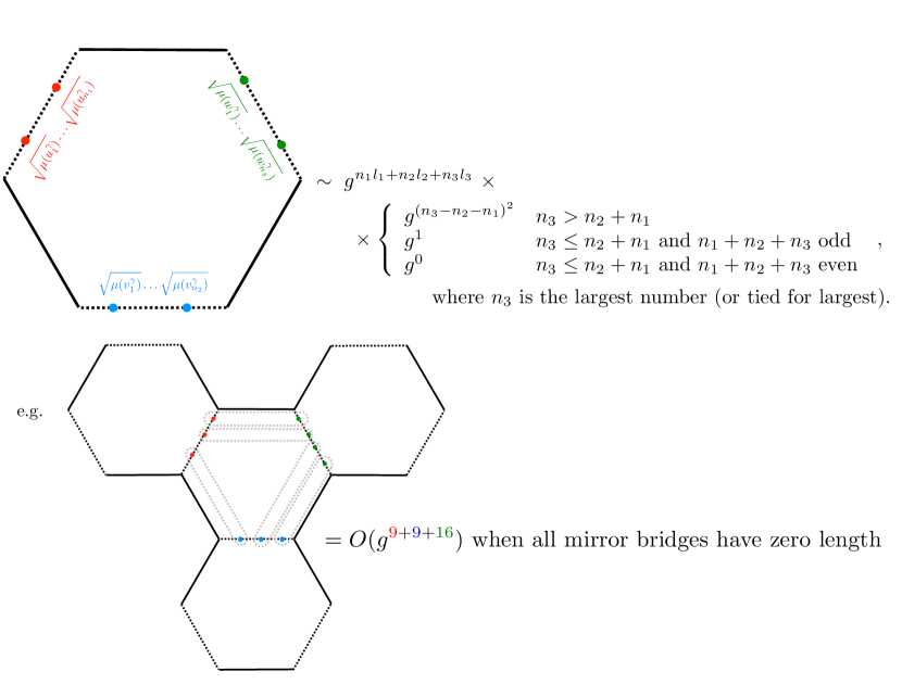
Figure 2: To estimate at which loop order a given sprinkling pattern will start contributing, we can focus on each hexagon. We absorb in each hexagon one half (i. e. the square root) of the measures and mirror particle propagation factors of the three adjacent mirror edges. We can then estimate the loop order of a given populated hexagon by noting that this object has residues where particles decouple among themselves. For example, the middle hexagon in the bottom picture must cost no coupling since it contains residues where all particles annihilate, leaving an empty hexagon whose expectation value is just $1$. In other words, in this example, what costs (a lot!) of loops is to create the particles in the surrounding hexagons; once they are created, they can freely propagate through the middle hexagon (e. g. following the interior of the dashed regions) and that costs no coupling at all. The general loop counting is presented for completeness at the top. It follows by noticing that after the decoupling, one is left with mirror particles only on one edge. The integrand for this case has a trivial matrix part due to the unitarity of the $S$ matrix, and it is a product ($i<j$) of terms $h(u_{i},u_{j})h(u_{j},u_{i})\sim g^{4}$, where $h$ is the hexagon dynamical factor. See the Appendices C and D for the two-particle case. See also [37].

The next step in our prescription is to tile all graphs of the polygonization with hexagon form factors, which we refer to as the hexagonalization of the correlator. For many of the maximal graphs, the hexagonalization is straightforward, as every face has three edges connecting three operators, giving room to exactly one hexagon. But some maximal graphs, and in particular graphs with fewer edges, include higher polygons, which have to be subdivided into several hexagons. A polygon with $m$ edges (and $m$ cusps) subdivides into $m-2$ hexagons, which are separated by $m-3$ zero-length bridges (ZLBs). In this way, the torus with four punctures always gets subdivided into eight hexagons. Later on, each of these hexagons will be dressed with virtual particles placed on the mirror edges or bridges which will generate the quantum corrections to the correlator under study, and which we refer to as sprinkling. The general counting of loop order involved in a general sprinkling is illustrated in Figure 2.

Let us illustrate the hexagonalization with an example. Take the maximal graph 1.1 of Table 1, and remove the horizontal lines in the middle, as well as the diagonal lines connecting the lower operator with the lower two corners. The resulting graph is depicted in Figure 3.

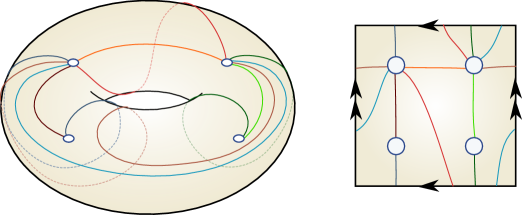
Figure 3: Skeleton graph obtained from maximal graph 1.1 by removing all horizontal lines and some diagonal connections as explained in the main text.

It has eight edges that divide the torus into four octagons. Each octagon gets subdivided into two hexagons by one zero-length bridge, as shown in Figure 4.

Figure 4: The skeleton graph of Figure 3 can be completed to a hexagonalization by inserting a zero-length bridge (ZLB, dashed lines) into each of the four octagons. This decomposes the four-punctured torus into eight hexagons.

In this case, the hexagonalization meant nothing but reinstating the deleted bridges as ZLBs. We can now draw the hexagon decomposition in a way that makes the hexagonal tiles more explicit. This results in the hexagon tiling shown in Figure 5.

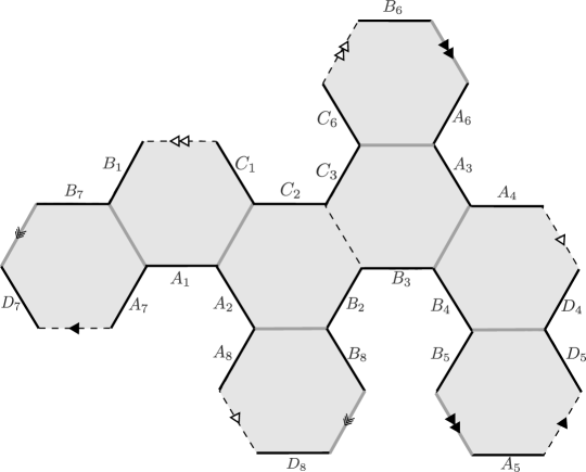
Figure 5: The hexagon tiling associated to the hexagonalization in Figure 4. The solid black lines attach to the four operators, the solid gray lines carry one or more propagators, and the dashed lines are zero-length bridges.

Dressing a skeleton graph such as the one in Figure 3 with ZLBs is not unique: Each octagon has two diagonals that we could choose to become ZLBs. The final answer will be independent of this choice. This property of the hexagonalization is called flip invariance [11]. Hence we can choose any way to cut bigger polygons into hexagons.

Ribbon Graph Automorphisms and Symmetry Factors.

When we perform the sum over all graphs and all bridge lengths on the torus (or higher-genus surface), we need to multiply some graphs by appropriate symmetry factors. The graphs we have been classifying are ribbon graphs. In order to understand the symmetry factors, we will take a closer look at the formal definition of these ribbon graphs. A ribbon graph is an ordinary graph together with a cyclic ordering of the edges at each vertex. More formally, ribbon graphs are defined through pairing schemes: Let $\mathcal{V}$ be a collection of non-empty ordered sets $V_{j}$,

$$\mathcal{V}=\{V_{1},\dots,V_{v}\}\,,\qquad V_{j}=(V_{j1},\dots,V_{j\ell_{j}})\,,$$ (2.15)

and let $\tilde{\mathcal{V}}=\{V_{11},\dots,V_{1\ell_{1}},\dots,V_{v1},\dots,V_{v\ell_{v}}\}$ be the union of all $V_{j}$. A pairing scheme $P=(\mathcal{V},p)$ is defined by a bijective pairing map $p:\tilde{\mathcal{V}}\to\tilde{\mathcal{V}}$ with $p^{2}=1$ and $p(V)\neq V$ for all $V\in\tilde{\mathcal{V}}$. Each ordered set $V_{j}$ of $P$ is called a vertex of $P$ of degree $\ell_{j}$. In our context, each vertex $V_{j}$ represents one of the operators, and the $V_{ji}$ label the (half-)bridges attached to operator $j$. The degree $\ell_{j}$ is the number of bridges attached to the operator. $P$ defines a ribbon graph, but also specifies a marked beginning of the ordered sequence of edges (bridges) attached to each vertex. Pairing schemes are promoted to ribbon graphs by the natural action of the group of orientation-preserving isomorphisms

$$G=\prod_{k=1}^{m}\mathrm{S}_{n_{k}}\rtimes(\mathbb{Z}/k\mathbb{Z})^{n_{k}}\,.$$ (2.16)

Here, $n_{k}$ is the number of vertices of degree $k$, $m$ is the maximal degree, $\mathrm{S}_{n_{k}}$ permutes vertices of the same degree, and $(\mathbb{Z}/k\mathbb{Z})^{n_{k}}$ rotates vertices of degree $k$. Each orbit $G.P$ of the group action defines a ribbon graph. In other words, a ribbon graph $\Gamma$ associated with a pairing scheme $P$ is the equivalence class of $P$ with respect to the action of $G$.

Typically an element of the group (2.16) maps a given pairing scheme $P$ to a different pairing scheme $P^{\prime}$ (by permuting vertices and/or shifting the marked beginnings of the ordered sequences of edges/bridges at each vertex/operator). However, some group elements may map a pairing scheme $P$ to itself. If $\Gamma$ is a ribbon graph associated with a pairing scheme $P$, then the subgroup of (2.16) preserving $P$ is called the automorphism group $\operatorname{Aut}(\Gamma)$ of $\Gamma$.

Assigning a positive real number to each edge of a ribbon graph promotes it to a metric ribbon graph. The number assigned to a given edge is called the length of that edge. Therefore, a graph with assigned bridge lengths is a metric ribbon graph (with integer edge lengths). The notion of automorphism group extends to metric ribbon graphs in an obvious way.

In the sum over graphs and bridge lengths, we need to divide each graph with assigned bridge lengths (metric graph) by the size of its automorphism group. These are the symmetry factors mentioned at the beginning of this paragraph.

Let us illustrate the idea with an example. Consider the following rather symmetric ribbon graph with eight edges, with all bridge lengths set to one:

$$\parbox[c]{43.362pt}{\includegraphics{FigTorusCasePmarked1}}\,\xrightarrow{g\in G}\,\parbox[c]{43.362pt}{\includegraphics{FigTorusCasePmarked2}}\,\xrightarrow{\text{shift}}\,\parbox[c]{43.362pt}{\includegraphics{FigTorusCasePmarked1}}$$ (2.17)

In the left picture, the graph is represented by an arbitrarily chosen pairing scheme, where the beginnings/ends of the edge sequences at each vertex are indicated by the small blue cuts. The second picture shows the pairing scheme obtained by applying an isomorphism $g\in G$ that cyclically rotates all vertices by two sites. In the second step, we shift the cycles along which we cut the torus in order to represent it in the plane. As a result, we see that the pairing scheme after applying $g$ is the same as the original pairing scheme on the left. Thus this graph has to be counted with a symmetry factor of $1/2$ (there is no other non-trivial combination of rotations that leave the graph invariant, and hence the automorphism group has size $2$). If we increase the bridge length on two of the edges to two, we find the following:

$$\parbox[c]{43.362pt}{\includegraphics{FigTorusCasePmarked3}}\,\xrightarrow{g\in G}\,\parbox[c]{43.362pt}{\includegraphics{FigTorusCasePmarked4}}$$ (2.18)

As can be seen from the pictures, applying the same group element to the original pairing scheme results in a different pairing scheme that cannot be brought back to the original by any trivial operation. In this case, the automorphism group is trivial, and the graph has to be counted with trivial factor $1$.

The symmetry factors can also be understood from the point of view of field contractions: When writing the sum over contractions as a sum over graphs and bridge lengths, we pull out an overall factor of $k^{4}$ that accounts for all possible rotations of the four single-trace operators. For some graphs and choices of bridge lengths, non-trivial rotations of the four operators can lead to identical contractions, which are thus over-counted by the overall factor $k^{4}$. This can be seen explicitly in the above example (2.17). Dividing by the size of the automorphism group exactly cancels this over-counting.

2.3 Stratification

The fact that we are basing the contribution at a given genus $g$ on the sum over graphs of genus $g$ is of course natural from the point of view of perturbative gauge theory: Each graph with assigned bridge lengths is equivalent to a Feynman graph of the free theory. Summing over graphs of genus $g$ and over bridge lengths (weighted by automorphism factors) is therefore equivalent to summing over all free-theory Feynman graphs of genus $g$. All perturbative corrections associated to a given graph are captured by the product of hexagon form factors as well as the sums and integrations over mirror states associated to that graph. It is clear that this prescription cannot be complete, as it does not include loop corrections that increase the genus of the underlying free graph. It also omits contributions from disconnected free graphs that become connected after adding interactions. In other words, it does not include contributions from handles or connections formed purely by virtual processes. We can include such contributions by drawing lower-genus and disconnected graphs on a genus-$g$ surface in all possible ways, and tessellating the genus-$g$ surface into hexagons including the handles not covered by the lower-genus graph. Weighting such contributions by the same genus-counting factor $N^{2-2g-n}$ as the honestly genus-$g$ graphs, we include all virtual processes that contribute at this genus. In other words, the sum over graphs in (LABEL:eq:mainformula) has to be replaced as

$$\sum_{\Gamma\in\mathbold{\Gamma}}=\sum_{g=0}^{\infty}\sum_{\begin{subarray}{c}\text{graphs }\Gamma\\ \text{of }{\text{genus }g}\end{subarray}}\qquad\rightarrow\qquad\sum_{g=0}^{\infty}\sum_{\Gamma\in\Sigma_{g}}\,,$$ (2.19)

where $\Sigma_{g}$ is the set of all graphs, connected or disconnected, of genus $g$ or smaller. For graphs whose genus is smaller than $g$, the symbol $\Gamma\in\Sigma_{g}$ has to carry not only the information of the graph itself, but also of its embedding in the genus-$g$ surface. The embedding can for example be encoded by marking all pairs of faces of the graph to which an extra handle is attached.

While this prescription solves the problem of capturing all genus-$g$ contributions, it also spoils the result by including genuine lower-genus contributions. Namely, the loop expansion of the hexagon gluing (sum over mirror states) will also include processes where one or more extra handles (those not covered by the graph) remain completely void. Such void handles can be pinched. Pinching a handle reduces the genus, hence such contributions do not belong to the genus-$g$ answer. However, we can get rid of these unwanted contributions by subtracting the same lower-genus graphs, but now drawn on a surface where a handle has been pinched. Pinching a handle reduces the genus by one, leaving two marked points on the reduced surface. For an $n$-point function, we hence have to subtract all $n$-point graphs drawn on a genus $(g-1)$ surface with $2$ marked points. Such contributions naturally come with the correct genus-counting factor $N^{2-2(g-1)-(n+2)}=N^{2-2g-n}$. Hence we have to refine (2.19) to

$$\text{RHS of~{}\eqref{eq:stratification1}}\quad\rightarrow\quad\sum_{g=0}^{\infty}\biggl{(}\sum_{\Gamma\in\Sigma_{g}}-\sum_{\Gamma\in\Sigma_{g-1}^{2}}\biggr{)}\,,$$ (2.20)

where $\Sigma_{g-1}^{2}$ is the set of all graphs of genus $(g-1)$ or smaller embedded in a genus $(g-1)$ surface, with two marked points inserted into any two faces of the graph (or both marked points inserted into the same face). This subtraction correctly removes all excess contributions from the first sum that have exactly one void handle. In contrast, the excess contributions with two void handles are contained twice in the subtraction sum, once for each handle that can be pinched. We have to re-add these contributions once by further refining (2.20) to

$$\text{RHS of~{}\eqref{eq:stratification2}}\quad\rightarrow\quad\sum_{g=0}^{\infty}\biggl{(}\sum_{\Gamma\in\Sigma_{g}}-\sum_{\Gamma\in\Sigma_{g-1}^{2}}+\sum_{\Gamma\in\Sigma_{g-2}^{4}}\biggr{)}\,,$$ (2.21)

where now $\Sigma_{g-2}^{4}$ is the set of all graphs of genus $(g-2)$ or smaller embedded in a genus $(g-2)$ surface, with two pairs of marked points inserted into any four (or fewer) faces of the graph. This procedure iterates, leading to the refinement

$$\text{RHS of~{}\eqref{eq:stratification3}}\quad\rightarrow\quad\sum_{g=0}^{\infty}\sum_{m=0}^{g}(-1)^{m}\sum_{\mathclap{\Gamma\in\Sigma_{g-m}^{2m}}}\,.$$ (2.22)

Under the degenerations discussed thus far, the Riemann surface stays connected. There are also degenerations that split the Riemann surface into two components by pinching an intermediate cylinder. Also these degenerations have to be subtracted in order to cancel unwanted contributions (that originate from disconnected propagator graphs, or from purely virtual “vacuum” loops). Such degenerations split a Riemann surface of genus $g$ with $n$ punctures into two components with genus $g_{1}$ and $g_{2}$ that contain $n_{1}$ and $n_{2}$ punctures, such that $g_{1}+g_{2}=g$ and $n_{1}+n_{2}=n$. Each component carries one marked point that remains from pinching. Such contributions also come with the correct genus-counting factor

$$N^{2-2g_{1}-(n_{1}+1)}N^{2-2g_{2}-(n_{2}+1)}=N^{2-2g-n}\,.$$ (2.23)

Again, the pinching process can iterate, splitting the surface into more and more components. We will comment on this type of contributions at the end of Section 5 and in Appendix F.

Summing all possible degenerations with their respective signs, we arrive at the following final formula, which is a further refinement of (2.22):

$$\text{RHS of~{}\eqref{eq:stratificationExtra}}\quad\rightarrow\quad\sum_{g=0}^{\infty}\sum_{c=1}^{2g+n-2}\mspace{-8.0mu}\sum_{\tau\in\mathbold{\tau}_{g,c,n}}\mspace{-3.0mu}(-1)^{\sum_{i}m_{i}/2}\sum_{\Gamma\in\Sigma_{\tau}}\equiv\mathcal{S}\circ\sum_{\Gamma\in\mathbold{\Gamma}}\,.$$ (2.24)

Here, $c$ counts the number of components of the surface, and the sum over $\tau$ runs over the set of all genus-$g$ topologies with $c$ components and $n$ punctures:

$$\mathbold{\tau}_{g,c,n}=\bigl{\{}\left\{(g_{1},n_{1},m_{1}),\dotsc,(g_{c},n_{c},m_{c})\right\}\big{|}\sum_{i}n_{i}=n\,,\;\sum_{i}(g_{i}+m_{i}/2)-c+1=g\bigr{\}}\,,$$ (2.25)

where $(g_{i},n_{i},m_{i})$ labels the genus, the number of punctures, and the number of marked points on component $i$. Finally, we sum over the set $\Sigma_{\tau}$ of all graphs $\Gamma$ (connected and disconnected) that are compatible with the topology $\tau$ and that are embedded in the surface defined by $\tau$ in all inequivalent possible ways ($\Gamma$ may cover all or only some components of the surface).

In the rightmost expression, we have defined the stratification operator $\mathcal{S}$, which implements the refinement of adding and subtracting graphs on surfaces of genus ${\leq}g$ with marked points as just explained. It appears intricate as it stands, but we will see below that it turns out less complicated than it looks.

We motivated this proposal from gauge theory considerations. We could have arrived at the very same expression by following string moduli space considerations as explained in the introduction, by carefully subtracting the boundary of the discretized moduli space [29, 30].

Example.

Let us illustrate the above construction with an important example. Consider the correlator for four equal-length single-trace operators $\mathcal{Q}_{1},\dots,\mathcal{Q}_{4}$ that are chosen such that the fields in $\mathcal{Q}_{1}$ cannot contract with the fields in $\mathcal{Q}_{4}$, and the fields in $\mathcal{Q}_{2}$ cannot contract with the fields in $\mathcal{Q}_{3}$. Correlators of this type are studied throughout the rest of this paper. For such correlators, there is only one planar graph:

$$\parbox[c]{36.8577pt}{\includegraphics{FigPlanarGraph}}\,.$$ (2.26)

At genus one, stratification requires that we include contributions from this graph drawn on a torus in all possible ways. An obvious way of drawing the planar graph on the torus is (the torus is drawn as a square, opposing sides of the square have to be identified)

$$\parbox[c]{43.362pt}{\includegraphics{FigTorusStrat1lab}}\,.$$ (2.27)

Pinching the handle of the torus leads back to the original graph drawn on the plane, with two marked points remaining where the handle got pinched:

$$\parbox[c]{43.362pt}{\includegraphics{FigTorusStrat1lab}}\quad\xrightarrow{\;\text{pinching}\;}\quad\parbox[c]{63.5976pt}{\includegraphics{FigTorusStrat1sublab}}\,.$$ (2.28)

According to the stratification prescription, the contribution from (2.27) has to be added, whereas the contribution from (2.28) (right-hand side) has to be subtracted in the computation of the genus-one correlator. Of course there are many more ways to draw the planar graph on a torus. Finding all such ways amounts to adding an empty handle to the planar graph in all possible ways. This in turn is equivalent to inserting two marked points into the planar graph in all possible ways, which mark the insertion points of the added handle. In other words, we can find all ways of drawing the planar graph on the torus by drawing graphs of the type shown on the right-hand side of (2.28). The two marked points can either be put into faces of the original graph, as in (2.28), but they can also be put inside bridges—a bridge stands for a collection of parallel propagators, hence it can be split in two by an extra handle. Going through all possibilities, we find the seven types of contributions listed in Table 2.

$\rightarrow$ $(1)$ $(1^{\prime})$ $\searrow$ $(1^{\prime\prime})$	$\rightarrow$ $(2)$ $(2^{\prime})$
$\rightarrow$ $(3)$ $(3^{\prime})$	$\rightarrow$ $(4)$ $(4^{\prime})$
$\rightarrow$ $(5)$ $(5^{\prime})$	$\rightarrow$ $(6)$ $(6^{\prime})$
$\rightarrow$ , $(7)$ $(7^{\prime})$ $(7^{\prime\prime})$

Table 2: List of stratification contributions for a genus-one four-point correlator $\langle\mathcal{O}_{1}\dots\mathcal{O}_{4}\rangle$ of equal-weight operators $\mathcal{O}_{1},\dotsc,\mathcal{O}_{4}$, where $\mathcal{O}_{1}$ cannot contract with $\mathcal{O}_{4}$, and $\mathcal{O}_{2}$ cannot contract with $\mathcal{O}_{3}$. Each case has to be summed over all inequivalent labelings of the four operators. Unprimed contributions $(i)$ are planar graphs drawn on a torus and thus have to be counted with a positive sign. Primed contributions $(i^{\prime})$ are obtained from their unprimed counterparts by pinching a handle and thus have to be counted with a negative sign. Doubly primed contributions $(i^{\prime\prime})$ are obtained by pinching off the entire torus, they also have to be counted with a negative sign.

In the table, we have listed unlabeled graphs, which have to be summed over inequivalent labelings. One may wonder why we have not included a variant of case (1) where the two marked points are “inside” the planar graph. In fact, this other case is included in the sum over labelings of case (1): Putting the two marked points “inside” the graph is equivalent to turning the graph (1) “inside out”, which amounts to reversing the cyclic labeling of the four operators. Similarly for case (3), the case where the exterior marked point sits inside the central face is included in the sum over labelings.

We will see below that mirror particle contributions may cancel propagator factors of the underlying free-theory graph. We therefore have to also sum over graphs containing propagators that are ultimately not admitted by the external operators. From an operational point of view, this is equivalent to only restricting the operator polarizations at the very end of the computation. For operators of equal weight but generic polarizations, the only planar four-point graph besides (2.26) is the “tetragon graph”

$$\raisebox{4.30554pt}{\parbox[c]{42.6393pt}{\includegraphics{FigPlanarGraphNonCyc}}}\;.$$ (2.66)

Putting this graph on a torus in all possible ways, we find eight inequivalent cases, listed in Table 3 and labeled $(8)$–$(15)$.

$\rightarrow$ , $(8)$ $(8^{\prime})$ $(8^{\prime\prime})$
$\rightarrow$ $(9)$ $(9^{\prime})$	$\rightarrow$ $(10)$ $(10^{\prime})$
$\rightarrow$ , $(11)$ $(11^{\prime})$ $(11^{\prime\prime})$
$\rightarrow$ $(12)$ $(12^{\prime})$	$\rightarrow$ $(13)$ $(13^{\prime})$
$\rightarrow$ $(14)$ $(14^{\prime})$	$\rightarrow$ $(15)$ $(15^{\prime})$

Table 3: Additional stratification contributions for a genus-one four-point correlator $\langle\mathcal{O}_{1}\dots\mathcal{O}_{4}\rangle$ of equal-weight operators $\mathcal{O}_{1},\dotsc,\mathcal{O}_{4}$ of generic polarizations. These have to be included even if some operators are polarized such that they ultimately cannot contract, because mirror particle contributions may cancel propagator factors of the underlying free graph.

For the graph (2.66), all faces are equivalent. Therefore, it is clear that all ways of placing one or two marked points into the several faces are equivalent (up to operator relabelings). Therefore, we include only one representative of all these variants. As for the cases listed in Table 2, the stratification prescription requires that the unprimed contributions should be added, while the primed contributions should be subtracted.

Thus far, we have accounted for pinchings where the handle of the torus becomes infinitely thin. However, for cases (1), (7), (8) and (11) there is another way to pinch, where one separates the whole torus from the graph, leaving an empty torus with one marked point, and the graph on a sphere with one marked point inside the face that previously contained the torus. These cases are labeled ($1^{\prime\prime}$), ($7^{\prime\prime}$), ($8^{\prime\prime}$) and ($11^{\prime\prime}$) in Table 2 and Table 3, and have to be subtracted as well.

For connected graphs, these two types of degenerations are all that can occur at genus one, since these are the only types of degenerations a torus admits, as illustrated in Figure 6 and Figure 7. Disconnected graphs do not contribute to any computation in this paper, and hence are not considered here.

To summarize, the effect of stratification at genus one, for correlators of the type considered here, is that the sum over genus-one graphs has to be augmented by a sum over the unprimed graphs (with positive sign) and a sum over the primed graphs (with negative sign) of Table 2 and Table 3:

$$\langle\mathcal{Q}_{1}\dotsc\mathcal{Q}_{4}\rangle^{(g=1)}=\Bigl{(}\begin{tabular}[]{@{}c@{}}{genus-one}\\ {graphs}\end{tabular}\Bigr{)}+\underbrace{\frac{k^{2}}{N_{\text{c}}^{4}}\sum_{i=1\vphantom{\}}}^{14}S_{(i)}}_{\begin{subarray}{c}\equiv\;\texttt{secretly}\\ \texttt{planar}\end{subarray}}\underbrace{\mbox{}-\frac{k^{2}}{N_{\text{c}}^{4}}\sum_{i=1}^{14}S_{(i^{\prime})}-\frac{k^{2}}{N_{\text{c}}^{4}}\sum_{i\in\{1,7,8,11\}}\mspace{-20.0mu}S_{(i^{\prime\prime})}}_{\equiv\;\texttt{subtraction}}\,,$$ (2.108)

where $S_{(i)}$, $S_{(i^{\prime})}$, and $S_{(i^{\prime\prime})}$ stand for the full contributions (sums over bridge lengths and mirror states) of the respective graphs. Note that, by construction, the genus-one stratification formula (2.108) is sufficiently general to hold for half-BPS operators $\mathcal{Q}_{i}$ of arbitrary polarizations $\alpha_{i}$ (but equal weights $k_{i}$).

2.4 Subtractions

We now explain how to compute the contributions from graphs associated with the degenerate Riemann surfaces, namely $(i^{\prime})$’s and $(i^{\prime\prime})$’s in Table 2 and Table 3.

Figure 6: Diagrammatic interpretation of marked points. (a) The diagram corresponding to the degenerate Riemann surface. (b) Pinching procedure. (c) The diagram after pinching. The red regions in (c) correspond to the marked points discussed in the previous subsection.

Marked Points as Holes in Planar Diagrams.

The first step of the computation is to better understand what the marked points ($\otimes$’s in Table 2) represent. For this purpose, it is useful to look at the corresponding Feynman graphs in the double-line notation. An example Feynman diagram that contributes to a stratification subtraction is depicted in Figure 6. Although drawn on a torus, it is essentially a planar diagram, and therefore corresponds to a degenerate Riemann surface. After the degeneration of the torus (see Figure 6(b)), the pinched handle becomes two red regions as shown in Figure 6(c), which are the faces of the original planar diagram. We thus conclude that, at the diagrammatic level, inserting two marked points on the sphere amounts to specifying two holes/faces of all planar Feynman graphs. For a planar graph $\mathcal{G}$ with $F$ faces, there are $\operatorname{Binomial}(F,2)=F(F-1)/2$ different ways of specifying two holes in two different faces of the graph. Thus the contribution of a graph with two marked points in different faces (denoted by $\mathcal{G}_{2\otimes}$) is given in terms of the contribution of the original graph $\mathcal{G}$ as

$$\mathcal{G}_{2\otimes}=\frac{F(F-1)}{2}\times\mathcal{G}\,,$$ (2.109)

where $F$ is the number of faces in $\mathcal{G}$. This provides a clear diagrammatic interpretation of the marked points, but it does not immediately tell us how to compute them using integrability, since one cannot in general isolate the contributions of individual Feynman diagrams in the integrability computation. To perform the computation, we need to relate them to yet another object that we discuss below.

The key observation is that the same factor $F(F-1)/2$ appears when we shift the rank of the gauge group: Consider the planar Feynman diagram $\mathcal{G}$ in U$(N_{\text{c}})$ $\mathcal{N}=4$ SYM, and change the rank from $N_{\text{c}}$ to $N_{\text{c}}+1$. Since each face of the planar diagram gives a factor of $N_{\text{c}}$, the shift of $N_{\text{c}}$ produces the following change in the final result

$$\mathcal{G}\quad\xrightarrow{\;N_{\text{c}}\to N_{\text{c}}+1\;}\quad\left(\frac{N_{\text{c}}+1}{N_{\text{c}}}\right)^{F}\mathcal{G}=\left(1+\frac{F}{N_{\text{c}}}+\frac{F(F-1)/2}{N_{\text{c}}^{2}}+\cdots\right)\mathcal{G}\,.$$ (2.110)

This offers a reasonably simple way to compute the contribution from the degenerate Riemann surface: Namely we just need to

1. Take the planar result and shift the rank of the gauge group from $N_{\text{c}}$ to $N_{\text{c}}+1$.

2. Expand it at large $N_{\text{c}}$ and read off the $1/N_{\text{c}}^{2}$ correction.

With this procedure, one can automatically obtain the correct combinatorial factor without needing to break up the planar results into individual Feynman diagrams.

Before applying this to our computations, let us add some clarifications: Firstly, when we shift $N_{\text{c}}$ to $N_{\text{c}}+1$, we keep the Yang–Mills coupling constant $g_{\scriptscriptstyle\mathrm{YM}}$ fixed, not the ’t Hooft coupling constant $\lambda=g_{\scriptscriptstyle\mathrm{YM}}^{2}N_{\text{c}}$. Put differently, we must shift the value of $\lambda$ when we perform the shift of $N_{\text{c}}$. Secondly, the planar correlators to which we perform the shift must be unnormalized: If we normalize the planar correlators so that the two-point function is unit-normalized, the shift of $N_{\text{c}}$ will no longer produce the correct combinatorial factor dependent on $F$.

It is now straightforward to evaluate the contribution from degenerate Riemann surfaces explicitly. The planar connected correlator for BPS operators of weights (lengths) $k_{i}$ admits the following expansion

$$G_{\{k_{1},\dotsc,k_{n}\}}^{(N_{\text{c}})}=N_{\text{c}}^{\mathcal{K}+2-n}\sum_{\ell=0}^{\infty}c_{\ell}\,\lambda^{\ell}\,,$$ (2.111)

where $c_{\ell}$ is a coefficient independent of $N_{\text{c}}$ and $\lambda$, and $\mathcal{K}=\sum_{i}k_{i}/2$. Shifting $N_{\text{c}}$ to $N_{\text{c}}+1$, we obtain

$$G_{\{k_{1},\dotsc,k_{n}\}}^{(N_{\text{c}}+1)}=N_{\text{c}}^{\mathcal{K}+2-n}\sum_{\ell=0}^{\infty}c_{\ell}\,\lambda^{\ell}\left[1+\frac{\mathcal{K}+2-n+\ell}{N_{\text{c}}}+\frac{1}{N_{\text{c}}^{2}}\begin{pmatrix}\mathcal{K}+2-n+\ell\\ 2\end{pmatrix}+\dots\right]$$ (2.112)

We thus conclude that the correlator $G_{\{k_{1},\dotsc,k_{n}\}}^{2\otimes}$ with two extra marked points inserted into two different faces in all possible ways is given by

$$\left.G_{\{k_{1},\dotsc,k_{n}\}}^{2\otimes}\right|_{O(\lambda^{\ell})}=\begin{pmatrix}\mathcal{K}+2-n+\ell\\ 2\end{pmatrix}\times\left.G_{\{k_{1},\dotsc,k_{n}\}}^{(N_{\text{c}})}\right|_{O(\lambda^{\ell})}\,.$$ (2.113)

Once we get this formula, we can then normalize both sides, since the normalization for BPS operators does not depend on $\lambda$.

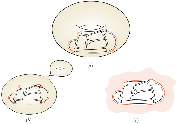
Figure 7: Degeneration to a single marked point. In addition to the degeneration shown in Figure 6, there is a yet another class of degenerations which produces a sphere with a single marked point. They correspond to the diagrams shown in (a) which degenerates into (c) depicted above. The red region in (c) corresponds to a marked point.

So far, we have been discussing the degeneration in which a handle degenerates into a pair of marked points. The other type of degeneration, in which the surface is split in two by pinching an intermediate cylinder, is exemplified in Figure 7. As shown in this figure, this type of degeneration produces a single marked point on the planar surface. Therefore, the analogue of (2.109) in those cases reads

$$\mathcal{G}_{\otimes}=F\mathcal{G}\,,$$ (2.114)

where again $F$ is the number of faces in the Feynman graph $\mathcal{G}$. The combinatorial factor $F$ in this case can also be related to the shift of $N_{\text{c}}$; namely it corresponds to the $O(1/N_{\text{c}})$ term in the expansion (2.110). We therefore conclude that the correlator with a single extra marked point is given by

$$\left.G_{\{k_{1},\dotsc,k_{n}\}}^{\otimes}\right|_{O(\lambda^{\ell})}=(\mathcal{K}+2-n+\ell)\times\left.G_{\{k_{1},\dotsc,k_{n}\}}^{(N_{\text{c}})}\right|_{O(\lambda^{\ell})}\,.$$ (2.115)

In total, the subtraction for a correlator on the torus at order $O(\lambda^{\ell})$ is given by

$$\left.(\texttt{subtraction})\right|_{O(\lambda^{\ell})}=\begin{pmatrix}\mathcal{K}+3-n+\ell\\ 2\end{pmatrix}\times\left.(\texttt{planar})\right|_{O(\lambda^{\ell})}$$ (2.116)

where (subtraction) denotes the subtraction piece while (planar) is a planar correlator.

Decomposition into Polygons at One Loop.

The formula above computes the full $k$-loop subtraction all at once. However, it is practically more useful to decompose the subtraction into the contributions associated with individual tree-level diagrams, so we can observe cancellations with other contributions more straightforwardly.

This can be done rather easily by generalizing the argument we just presented: As shown in Table 2, the degeneration of a Riemann surface with a tree-level graph leads to polygons (i. e. faces) with one or two marked points. To evaluate these polygons, we just need to keep in mind that each polygon admits the expansion

$$(\mathop{\texttt{polygon}})=N_{\text{c}}\sum_{\ell}p_{\ell}\,\lambda^{\ell}\,.$$ (2.117)

The overall factor $N_{\text{c}}$ comes from the fact that the edges of the polygon constitute a closed index-loop. Although we do not normally associate such a factor with each polygon, here it is crucial to include that factor to count the faces correctly.

The rest of the argument is identical to the one before: Shifting $N_{\text{c}}$ to $N_{\text{c}}+1$ and reading off the $1/N_{\text{c}}$ and $1/N_{\text{c}}^{2}$ terms, we get

$$(\mathop{\texttt{polygon}})_{\otimes}\big{|}_{O(\lambda^{\ell})} =(1+\ell)\times(\mathop{\texttt{polygon}})\big{|}_{O(\lambda^{\ell})}\,,$$ (2.118)

$$(\mathop{\texttt{polygon}})_{2\otimes}\big{|}_{O(\lambda^{\ell})} =\frac{(1+\ell)\ell}{2}\times(\mathop{\texttt{polygon}})\big{|}_{O(\lambda^{\ell})}\,.$$

Here $(\mathop{\texttt{polygon}})_{\otimes}$ and $(\mathop{\texttt{polygon}})_{2\otimes}$ denote the contributions from a polygon with one or two marked points respectively. Using the fact that the $O(\lambda^{0})$ term for each polygon is just unity, one can also write an explicit weak-coupling expansion as

$$(\mathop{\texttt{polygon}})_{\otimes} =1+2(\mathop{\texttt{polygon}})\big{|}_{O(\lambda)}+\dots\,,$$ (2.119)

$$(\mathop{\texttt{polygon}})_{2\otimes} =0+(\mathop{\texttt{polygon}})\big{|}_{O(\lambda)}+\dots\,.$$

These formulae will be used intensively below.

Worldsheet Interpretation.

Let us end our discussion on the subtraction by mentioning the worldsheet interpretation of the marked points. This is more or less obvious from the way we performed the computation: Shifting the rank of the gauge group from $N_{\text{c}}$ to $N_{\text{c}}+1$ amounts to adding a probe D3-brane in AdS. It is well-known that the probe brane sitting at some finite radial position $z$ describes the Coulomb branch of $\mathcal{N}=4$ SYM, in which the gauge group is broken from ${\rm U}(N_{\text{c}}+1)$ to ${\rm U}(N_{\text{c}})\times{\rm U}(1)$. In our case, we are not breaking any conformal symmetry, and therefore the probe brane must sit at the horizon of AdS ($z=\infty$ in Poincaré coordinates).

This suggests that the marked points that we have been discussing correspond to boundary states describing the probe brane at the horizon. Furthermore, our computation (2.115) implies that the $n$-point tree-level string amplitude with an insertion of a hole is related to the same amplitude without insertion as

$$\lambda^{\mathcal{K}-2+n}A_{\text{sphere+hole}}=\frac{\partial}{\partial\lambda}\left(\lambda^{\mathcal{K}-2+n}A_{\text{sphere}}\right)\,.$$ (2.120)

It would be interesting to verify this prediction by a direct worldsheet computation.

Let us finally add that, although the argument above gives a worldsheet interpretation of the marked points, it does not explain why such boundary states are relevant for the analysis of the degenerate worldsheet. It would be desirable to find a worldsheet explanation for this, which does not rely on the Feynman-diagrammatic argument presented in this section.

2.5 Dehn Twists and Modular Group

The backbone of our formula (LABEL:eq:mainformula) is a summation over (skeleton) graphs. When we construct the complete set of graphs on a surface of given genus, we implicitly identify graphs that only differ by “twists” of a handle. For example, we treat the genus-one graphs

   and    (2.121)

as identical. This makes perfect sense from a weak-coupling perturbative point of view: Wick contractions only carry information about the ordering of bridges around each operator, not on the particular way in which the graph is embedded in a given surface. Hence the two graphs (2.121) are identical as Feynman graphs. Modding out by such twists is also natural from the string-worldsheet perspective. The summation over graphs represents the integration over the moduli space of complex structures of the string worldsheet. The “twists” mentioned above are called Dehn twists. More formally, a Dehn twist is defined as an operation that cuts a cylindrical piece (the neighborhood of a cycle) out of a Riemann surface (the worldsheet), performs a $2\pi$ twist on this piece, and glues it back in, see Figure 8.

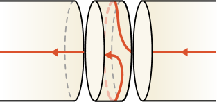
Figure 8: Dehn twists: Left: In red, we represent a path along the worldsheet that undergoes a complete cycle in the cylindrical piece where a Dehn twist was performed. Middle and Right: Stratification contributions that get added (graph on a torus, middle figure) and subtracted (planar graph with marked points, right figure), with shaded regions that form non-trivial cycles, on which one can perform Dehn twists that leave the embedding of the graph invariant.

Such Dehn twists leave the complex structure of the Riemann surface invariant, and hence should be modded out by when integrating over the moduli space. In fact, Dehn twists are isomorphisms that are not connected to the identity. They form a complete set of generators for the modular group (mapping class group) for surfaces of any genus and with any number of operator insertions (boundary components). Since all Dehn twists act as identities in the moduli space as well as on Feynman diagrams, it is natural to mod out by Dehn twists in all stages of the computation.

While modding out by Dehn twists is natural and straightforward in the summation over free-theory graphs (as we have been doing implicitly), it has non-trivial implications for the summation over mirror states, especially for the stratification contributions. By their nature, all stratification contributions contain non-trivial cycles that do not intersect with the graph of propagators: For the terms that get added, non-trivial cycles can wind the handles not covered by the graph, and for the terms that get subtracted, non-trivial cycles can wind around the isolated marked points (see Figure 8 for examples). Obviously, performing a Dehn twist on a neighborhood of such cycles neither alters the graph itself, nor its embedding in the surface. But once we fully tessellate the surface by a choice of zero-length bridges (and dress them with mirror magnons), such Dehn twists will alter (twist) the embedding of those bridges (ZLBs) on the surface. For example, the two graphs

   and    (2.122)

are related by a Dehn twist on a vertical strip in the middle of the picture, which only acts on the zero-length bridges (dashed lines). Since we anyhow do not sum over different ZLB-tessellations, but rather just pick one choice of ZLBs for each propagator graph, it looks like such twists need not concern us. However, notice that one can always transform a Dehn-twisted configuration of ZLBs back to the untwisted configuration via a sequence of flip moves on the ZLBs. As long as all participating mirror states are vacuous, these flip moves are trivial identities. However, as soon as we dress the ZLBs (and other bridges) with mirror magnons, flip moves will non-trivially map (sets of) excitation patterns, i. e. distributions of mirror magnons, to each other. Hence we have the situation that a given distribution of mirror magnons on a fixed choice of ZLB-tessellation might secretly be related to another distribution (or set of distributions) of magnons on the same, but now Dehn-twisted ZLB-tessellation. Since part of our interpretation of the sums over mirror magnons is that they probe the neighborhood of the discrete point in the moduli space represented by the underlying propagator graph, it seems natural to identify distributions of mirror magnons that are related in the way just described. We are therefore led to add the following element to our prescription:

Among all mirror-magnon contributions that are related to each other via Dehn twists followed by sequences of bridge flips, take only one representative into account. In other words, all mirror-magnon contributions that are related to each other via Dehn twists and sequences of bridge flips are identified. (2.123)

The one-loop evaluation of all relevant stratification contributions in Section 5 will lend quantitative support to this prescription.

3 Multi-Particles and Minimal Polygons

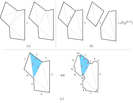
Figure 9: (a) An example of a minimal polygon. A minimal polygon is by definition a polygon that when triangulated/hexagonalized only contains zero-length bridges. This means that all internal mirror edges contribute at one-loop order if one inserts a mirror particle on them. It can be hexagonalized in several different ways, and all ways of doing so should give the same integrability result when summing over mirror particles. (b) A general polygon may have zero-length and non-zero-length bridges, and it can be divided into minimal polygons. Inserting mirror particles in non-zero-length bridges is more costly at weak coupling. (c) Two different ways of defining a polygon with physical operators on its edges. It is possible to shrink the operators to points or to blow them up to finite size. In the first case the surface is triangulated (only mirror edges), and in the second case it is hexagonalized (as many physical as mirror edges).

We think of a polygon as the inside of the face of a larger Feynman diagram, with the outer edges being propagators in that diagram. Depending on whether we blow up the physical operators or not, the same polygon can be either thought of as an $n$-gon (with $n$ mirror edges), or a $2n$-gon (with $n$ mirror edges and $n$ physical edges), as illustrated in Figure 9c. When we do blow up the physical operators we speak of hexagonalizing the polygon, otherwise we say that we triangulate it. In the hexagonalization picture, every other edge of each hexagon is formed by a segment (in color space) of a physical operator. In the triangulation picture, the physical operators sit at the cusps of the triangles. Of course, both pictures describe the very same thing, as indicated in Figure 9c.

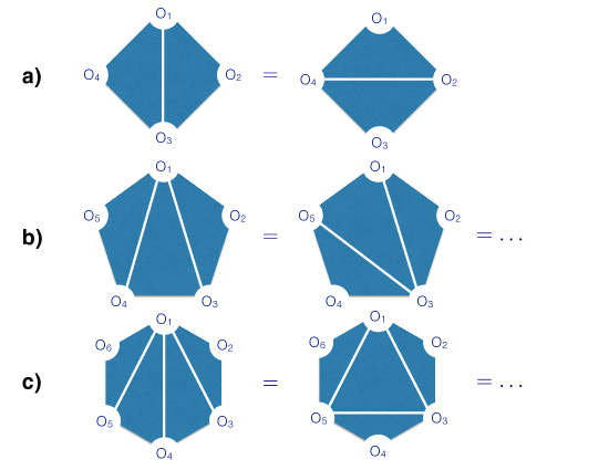
Figure 10: (a) An octagon and its two possible tessellations related by flipping and studied in [11]. (b) A decagon and its various tessellations studied in [14]. (c) The dodecagon has a few new features compared to the previous two examples. Here, different tessellations can be computed by very different integrability processes, with different numbers of mirror particles involved, see Figure 11.

There can be non-zero-length bridges in the interior of the polygon, as indicated in Figure 9b. When computing the expectation value of a polygon, we triangulate/hexagonalize it and insert mirror particles at all the mirror edges. When these edges are such non-zero-length bridges, this is more costly at weak coupling, as indicated in Figure 9b, so the expectation value of such polygons breaks down into polygons where all internal bridges have zero length. We call such polygons minimal polygons. For large bridges, this decomposition holds up to a large number of loops. In this paper, we focus only on such minimal polygons, such as the one in Figure 9a.

A minimal polygon can be hexagonalized in different ways, as illustrated in Figure 9a, and an important consistency condition is that all these tessellations ought to give the same result. Three further examples are illustrated in Figure 10. The first was considered in [11], the second in [14], and the third will be discussed later in this paper.

Variables.

Minimal polygons are functions of the labels of the physical operators at their perimeter, namely of the operator positions $x_{i}$ and internal polarizations $\alpha_{i}$ (for minimal polygons, the operator weights $k_{i}$ are irrelevant). Due to conformal symmetry and R-symmetry, minimal polygons can only be functions of spacetime cross ratios and cross ratios formed out of the internal polarizations. In this paper, we focus on four-point functions, and will use the familiar variables

$$z\bar{z}=\frac{x_{12}^{2}\,x_{34}^{2}}{x_{13}^{2}\,x_{24}^{2}}\,,\qquad(1-z)(1-\bar{z})=\frac{x_{14}^{2}\,x_{23}^{2}}{x_{13}^{2}\,x_{24}^{2}}\,,\qquad x_{ij}\equiv|x_{i}-x_{j}|\,.$$ (3.1)

For cross ratios of the internal polarizations, we similarly choose

$$\alpha\bar{\alpha}=\frac{(\alpha_{1}\cdot\alpha_{2})(\alpha_{3}\cdot\alpha_{4})}{(\alpha_{1}\cdot\alpha_{3})(\alpha_{2}\cdot\alpha_{4})}\,,\qquad(1-\alpha)(1-\bar{\alpha})=\frac{(\alpha_{1}\cdot\alpha_{4})(\alpha_{2}\cdot\alpha_{3})}{(\alpha_{1}\cdot\alpha_{3})(\alpha_{2}\cdot\alpha_{4})}\,.$$ (3.2)

In the following, we will consider more general minimal polygons that depend on $n$ external operators. However, we will restrict all operators to lie in the same plane, in spacetime as well as in the internal polarization space, as this is sufficient for our purposes. For every choice of four operators, we can form spacetime and polarization cross ratios exactly as in (3.1) and (3.2), and an $n$-point polygon in these restricted kinematics depends on $(n-3)$ sets of such cross ratios.

3.1 One-Loop Polygons and Strings from Tessellation Invariance

To fully compute a $2n$-gon vacuum expectation value, we should insert any number of mirror particles at all hexagon junctions and integrate over their rapidities. At one-loop order, things simplify: According to the loop-counting shown in Figure 2, we only need to sum over multi-particle strings which are associated to paths that connect one hexagon to another, never passing twice through the same hexagon. To construct the corresponding multi-particle string, we insert exactly one mirror particle whenever the path intersects a mirror edge. In sum, the one-loop $2n$-gon is obtained by picking a tessellation at one’s choice, and summing over all multi-particle one-loop strings on that tessellation. See Figure 11 for an example.

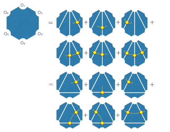
Figure 11: A tessellation of the dodecagon can contain paths where a mirror particle propagates through four different hexagons, as illustrated in the last graph in the second line. In another tessellation, a particle can propagate for at most three hexagons, as illustrated in the second example. Equating both, we can read off the larger propagation (three-particle) contribution from the smaller ones (two-particle and one-particle), as shown in (3.5).

Each mirror edge joins two hexagons into an octagon involving four operators. Hence two cross ratios are associated to each mirror edge in a natural way. For a mirror line $i$ connecting operator $\mathcal{O}_{a}$ with $\mathcal{O}_{c}$, where the two adjacent hexagons further connect to operators $\mathcal{O}_{b}$ and $\mathcal{O}_{d}$, we define the variable $z_{i}$ parametrizing the associated cross ratios as (note the dependence on the orientation of the sequence of operators around the perimeter)

$$\parbox[c]{49.1436pt}{\includegraphics{FigCrossRatios}}\;\;:\qquad z_{i}\bar{z}_{i}=\frac{x_{ab}^{2}\,x_{cd}^{2}}{x_{ad}^{2}\,x_{bc}^{2}}\,,\qquad(1-z_{i})(1-\bar{z}_{i})=\frac{x_{ac}^{2}\,x_{bd}^{2}}{x_{ad}^{2}\,x_{bc}^{2}}\,.$$ (3.3)

The corresponding polarization cross ratios are defined accordingly. With these definitions, we denote the contribution of a multi-particle one-loop string traversing $n$ mirror edges as

$$\mathcal{M}^{(n)}(z_{1},\dotsc,z_{n})\,,$$ (3.4)

where the variables $z_{i}$ parametrize the cross ratios associated to the $n$ mirror edges as in (3.3), and we are suppressing the obvious dependencies on $\bar{z}_{i}$ and the polarization cross ratios.

By exploiting the above-mentioned invariance under tessellation choice, one can determine the contribution from any multi-particle string $\mathcal{M}^{(n)}$ from the knowledge of the one- and two-particle contributions alone. As an illustration, consider the dodecagon example in Figure 11. In the second tessellation, only two-particle strings appear, while for the first tessellation, the sum includes a contribution with three particles. Equating both sums, we can relate the three-particle contribution to the one- and two-particle strings as

$$\mathcal{M} {}^{(3)}(z_{1},z_{2},z_{3})=$$

$$-\left(\mathcal{M}^{(1)}(z_{1})+\mathcal{M}^{(1)}(z_{2})+\mathcal{M}^{(1)}(z_{3})+\mathcal{M}^{(2)}(z_{1},z_{2})+\mathcal{M}^{(2)}(z_{2},z_{3})\right)$$

$$+\mathcal{M}^{(1)}\left(\frac{1}{z_{2}}\right)+\mathcal{M}^{(1)}\bigl{(}z_{1}(1-z_{2})\bigr{)}+\mathcal{M}^{(1)}\left(\frac{z_{2}z_{3}}{z_{2}-1}\right)+\mathcal{M}^{(2)}\left(\frac{1}{z_{2}},z_{1}(1-z_{2})\right)$$

$$+\mathcal{M}^{(2)}\left(z_{1}(1-z_{2}),\frac{z_{2}z_{3}}{z_{2}-1}\right)+\mathcal{M}^{(2)}\left(\frac{z_{2}z_{3}}{z_{2}-1},\frac{1}{z_{2}}\right)\,.$$ (3.5)

Here, the variables $z_{1}$, $z_{2}$, and $z_{3}$ parametrize the cross ratios associated to the three mirror edges of the first tessellation in Figure 11 (from right to left). Hence, $\mathcal{M}^{(1)}(z_{1})$ equals the first contribution in Figure 11, $\mathcal{M}^{(1)}(z_{2})$ equals the second contribution, and so on. In the above expression, it is implicit that the other, suppressed variables undergo the same substitutions as the $z_{i}$ variables, e. g.

$$\mathcal{M}^{(1)}\left(\frac{z_{2}z_{3}}{z_{2}-1}\right)\equiv\mathcal{M}^{(1)}\left(\frac{z_{2}z_{3}}{z_{2}-1},\frac{\bar{z}_{2}\bar{z}_{3}}{\bar{z}_{2}-1},\frac{\alpha_{2}\alpha_{3}}{\alpha_{2}-1},\frac{\bar{\alpha}_{2}\bar{\alpha}_{3}}{\bar{\alpha}_{2}-1}\right)\,,$$ (3.6)

where we have, by slight abuse of notation, used $(\alpha_{i},\bar{\alpha}_{i})$ to parametrize the polarization cross ratios. Using the explicit known results for one and two particles [11, 14]

$$\mathcal{M}^{(1)}(z) =m(z)+m(z^{-1})\,,$$ (3.7)

$$\mathcal{M}^{(2)}(z_{1},z_{2}) =m\left(\frac{z_{1}-1}{z_{1}z_{2}}\right)+m\left(\frac{1-z_{1}+z_{1}z_{2}}{z_{2}}\right)+m\bigl{(}z_{1}(1-z_{2})\bigr{)}-m(z_{1})-m(z_{2}^{-1})\,,$$

we find for the three-particle one-loop string:

$$\mathcal{M}^{(3)}(z_{1},z_{2},z_{3})=m\left(\frac{1-z_{1}+z_{1}z_{2}}{z_{1}z_{2}z_{3}}\right)+m\bigl{(}z_{1}(1-z_{2}+z_{2}z_{3})\bigr{)}\\ +m\left(\frac{(1-z_{2})(-1+z_{1}-z_{1}z_{2}+z_{1}z_{2}z_{3})}{z_{2}z_{3}}\right)-m\bigl{(}z_{1}(1-z_{2})\bigr{)}-m\left(\frac{z_{2}-1}{z_{2}z_{3}}\right)\,.$$ (3.10)

The cross ratios appearing in the argument of the three-particle contribution are defined as in (3.3). Here, the main building block function $m(z)$ is given by

$$m(z)\equiv g^{2}\,\frac{(z+\bar{z})-(\alpha+\bar{\alpha})}{2}F^{(1)}(z,\bar{z})\,,$$ (3.11)

with the one-loop conformal box integral

$$F^{(1)}(z,\bar{z})=\frac{1}{z-\bar{z}}\left(2\operatorname{Li}_{2}(z)-2\operatorname{Li}_{2}(\bar{z})+\log(z\bar{z})\log\left(\frac{1-z}{1-\bar{z}}\right)\right)\,.$$ (3.12)

The building block function $m(z)$ satisfies the following important identities:

$$m(0)=m(1)=m(\infty)=0\,,\qquad m(z)+m(1-z)=0\,.$$ (3.13)

Note that there is another type of three-particle contribution besides the one discussed above. It appears in an “alternating” tessellation of the same dodecagon:

$$\parbox[c]{286.1892pt}{\includegraphics[trim=0.0pt 469.47046pt 0.0pt 14.22636pt,scale={0.50}]{alternatingOrNot}}\,.$$ (3.14)

The “alternating cusp” three-particle string can be derived in the same way as the “common cusp” string by equating the alternating tessellation to one of the two tessellations shown in Figure 11.

By playing with tessellations of higher $2n$-gons in a similar way, we can derive, in the fashion described above, all multi-particle one-loop contributions, and therefore also all higher polygon one-loop expectation values in terms of contributions involving only one-particle and two-particle strings. Writing the latter in terms of the building block function $m(z)$ via (3.7), the resulting expression for a general $2n$-gon, for instance, is remarkably simple and reads

$$\mathop{\texttt{polygon}}(1,\dotsc,2n)=\sum_{\begin{subarray}{c}[i,i+1],[j,j+1]:\\ \text{non-consecutive}\end{subarray}}m\left(z_{i,j}\equiv\frac{x_{i,j+1}x_{i+1,j}}{x_{i,i+1}x_{j+1,j}}\right)\,.$$ (3.15)

We illustrate the formula in Figure 12 for the example of a decagon.

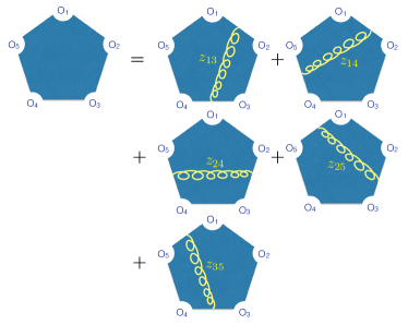
Figure 12: A $2n$-gon decomposes into a sum of gluon exchange-like contributions between all non-neighboring edges, with each exchange given by a function $m(z_{ij})$, as shown in (3.15).

In writing (3.15), we cyclically identified the operator labels, namely $n+1\equiv 1\mod n$. The sum runs over all possible pairs of non-consecutive edges at the perimeter, $[i,i+1]$ and $[j,j+1]$. Roughly speaking, the sum in (3.15) corresponds to a summation of all possible gluon-exchange diagrams that one can draw inside the $n$-point graph. This general result can actually be proved by induction, as illustrated in Figure 13.

Figure 13: Proof of (3.15) by induction for an even number of external edges. For an odd number, a proof can be found in a similar way. The combination in the first line amounts to the statement that all strings in such symmetric tessellations can probe zero, one, or two outer triangles. In order to probe more than two triangles, the string would have to bifurcate. All possible strings are of course contained in the first sum, but there is an obvious over-counting, which is removed by the last two terms.

3.2 Tests and Comments

We conclude this section with some further checks and comments.

Flip Invariance

We have assumed tessellation invariance to derive the $2n$-gon formula (3.15). Consistently, the result makes no reference to a particular tessellation, hence it is manifestly invariant under tessellation choice.

Order Invariance

We can think of each multi-particle string contribution as a mirror-particle propagation. The direction of propagation ought to be irrelevant, provided we properly read off the cross ratios for the associated process as in (3.3). This translates into

$$\mathcal{M}^{(2)}(z_{1},z_{2})=\mathcal{M}^{(2)}(z_{2}^{-1},z_{1}^{-1})\,,\quad\mathcal{M}^{(3)}(z_{1},z_{2},z_{3})=\mathcal{M}^{(3)}(z_{3}^{-1},z_{2}^{-1},z_{1}^{-1})\,,\quad\dots\,,$$ (3.16)

which we can indeed verify using the explicit formulas.

Reduction to Known $2n$-Gons

For the octagon $(n=4)$, there are two different pairs of non-consecutive edges; $[1,2],[3,4]$ and $[4,1],[2,3]$. It is easy to see that these two contributions lead to $m(z)$ and $m(z^{-1})$ respectively. Therefore, we recover the previous result [11]. Similarly, one can check that our formula reproduces the result for the decagon $(n=5)$. In this case, there are five different pairs of non-consecutive edges, and they correspond to the five terms in the decagon [14] represented in Figure 12:

$$\mathcal{M}^{(1)}(z_{1})+\mathcal{M}^{(1)}(z_{2})+\mathcal{M}^{(2)}(z_{1},z_{2})=\\ m(z_{1}^{-1})+m(z_{2})+m\left(\frac{z_{1}-1}{z_{1}z_{2}}\right)+m\left(\frac{1-z_{1}+z_{1}z_{2}}{z_{2}}\right)+m\bigl{(}z_{1}(1-z_{2})\bigr{)}\,.$$ (3.19)

OPE Limit

Starting from the dodecagon, one should be able to recover the result for the decagon by taking the limit $z_{3}\to 0$. This can be easily seen by using the properties (3.13). Since the result is manifestly flip-invariant, any OPE limit is essentially equivalent and has a good behavior.

Extremal and Next-to-Extremal Correlators

The $n$-point extremal and next-to-extremal correlators have non-renormalization properties [40, 41, 42]. Using our conjectural form of the $2n$-gon contribution, one can verify that the one-loop corrections are zero for those kinds of correlators, see Appendix E for details of the planar case.

Decoupling Limit

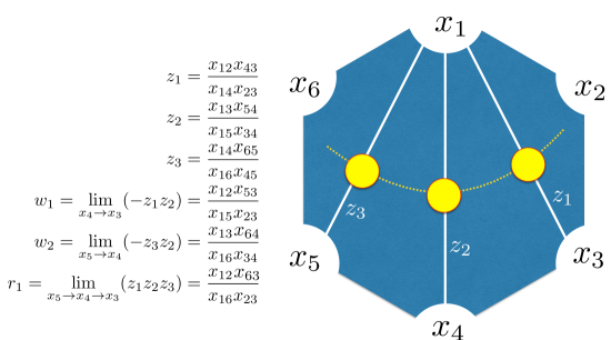
Figure 14: A dodecagon and its cross ratios. Collapsing $x_{i+1}\to x_{i}$ eliminates a slice – a hexagon – in the figure. The double limit $x_{i+2}\to x_{i+1}\to x_{i}$ reduces a $2n$-gon to a $2(n-2)$-gon. Mirror-state propagations in such polygons are reduced accordingly. From a form factor point of view, the corresponding sums collapse into the coinciding rapidity region.

We can reduce multi-particle strings to strings involving less steps by collapsing hexagons in the tessellation. For example, if we take $x_{4}\to x_{3}$ in Figure 14, we reduce the dodecagon to a decagon, and correspondingly the three-particle contribution reduces to a two-particle contribution. If we further send $x_{5}\to x_{4}\to x_{3}$, we reduce it further to an octagon, and we end up with a single-particle contribution. When taking these limits, some cross ratios diverge and others vanish. For example, $x_{4}\to x_{3}$ corresponds to $z_{1}/z_{2}\to 0$ with $z_{1}z_{2}=-w_{1}$ fixed. In this limit, we nicely find indeed

$$\mathcal{M}^{(3)}(z_{1},z_{2},z_{3})\to\mathcal{M}^{(2)}(w_{1},z_{3})\,,\qquad\text{as }z_{1}/z_{2}\to 0\text{ with }z_{1}z_{2}=-w_{1}\text{ fixed}\,,$$ (3.20)

in perfect agreement with the above expectations. From the integrability/form-factor point of view, this limit corresponds to the so-called decoupling limit, where consecutive rapidities are forced to become equal, and the corresponding hexagons collapse into measures and disappear. Similarly, we find

$$\mathcal{M}^{(3)}(z_{1},z_{2},z_{3}) \to\mathcal{M}^{(2)}(z_{1},w_{2})\,, \text{as }z_{2}/z_{3} \to 0\text{ with }z_{2}z_{3}=-w_{2}\text{ fixed}\,,$$

$$\mathcal{M}^{(2)}(z_{1},w_{2}) \to\mathcal{M}^{(1)}(r_{1})\,, \text{as }z_{1}/w_{2} \to 0\text{ with }z_{1}w_{2}=-r_{1}\text{ fixed}\,,$$

and many other similar relations at higher points.

Pinching at One Loop

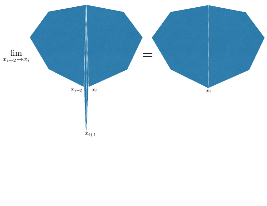
Figure 15: Pinching at one loop. As a consequence of both the form of the 2$n$-gon and the properties of the function $m(z)$, the limit when the cusps at position $i$ and $i+2$ have the same position $x_{i}$ equals a smaller polygon with two fewer cusps. This limiting polygon does not depend on the position and $R$-charge of the initial middle cusp $i+1$.

Another nice limit of any polygon is the one where cusps $i$ and $i+2$ go to the same position. When doing so, they pinch the edge ending at cusp $i+1$ and basically remove it, as illustrated in Figure 15. This limit removes all traces of the operator which got sandwiched between cusps $i$ and $i+2$,

$$\lim_{x_{i+2}\to x_{i}}\mathop{\texttt{polygon}}(x_{1},\dots,{\color[rgb]{1,0,0}x_{i}},{\color[rgb]{0,0,1}x_{i+1}},{\color[rgb]{1,0,0}x_{i+2}},\dots,x_{n})=\mathop{\texttt{polygon}}(x_{1},\dots,{\color[rgb]{1,0,0}x_{i}},\dots,x_{n})\,.$$ (3.21)

This identity is actually quite powerful and very useful for us. For four-point functions, for instance, all cusps are located at one of the four possible space-time insertions, so there will naturally be many repetitions of labels, which can be reduced with this rule. For example:

$$\mathop{\texttt{polygon}}(1,{\color[rgb]{0,0,1}2},{\color[rgb]{1,0,0}3},{\color[rgb]{0,0,1}2},4,3,1,{\color[rgb]{0,0,1}3},{\color[rgb]{1,0,0}2},{\color[rgb]{0,0,1}3})\to\mathop{\texttt{polygon}}({\color[rgb]{0,0,1}1},{2},4,3,{\color[rgb]{0,0,1}1},{\color[rgb]{1,0,0}3})\to\mathop{\texttt{polygon}}(2,4,3,1)\,.$$ (3.22)

For four-point functions, we can use the following simple Mathematica code to simplify arbitrary one-loop polygons:

⬇

polygon[L_] := Block[

{n=Length[L], x={-1,1/(2z-1),1,0}[[ L[[ Mod[#,n,1] ]] ]]&},

Sum[

m[(x[i]-x[j+1])(x[i+1]-x[j])/((x[i]-x[i+1])(x[j+1]-x[j])) // Simplify],

{i, 1, n}, {j, i+2, n-Boole[i==1]}

] /. {

m[1-z] -> -m[z], m[(-1+z)/z] -> -m[1/z],

m[z/(-1+z)] -> -m[1/(1-z)], m[0] -> 0, m[1] -> 0

}]

It implements (3.15), taking into account the functional identities (3.13) of the $m(z)$ building block. Running polygon[{1,2,3,2,4,3,1,3,2,3}], for instance, would simply yield $m(z)+m(1/z)$, which is the very same as polygon[{2,4,3,1}], as expected according to (3.22).

One-Loop Octagons

Below, we will need the expressions for one-loop octagons, hence we will quote them here. The one-loop octagon was computed in [11]. Due to the dihedral symmetry of the one-loop polygons (3.15), permutations of the four corners generate only three independent functions, corresponding to the orderings 1–2–4–3, 1–2–3–4, and 1–3–2–4 of the four operators around the perimeter of the octagon. Permutations of the four operators are generated by the following variable transformations:

$$3 \leftrightarrow 4: z \leftrightarrow\frac{z}{z-1}\,, \bar{z} \leftrightarrow\frac{\bar{z}}{\bar{z}-1}\,, \alpha \leftrightarrow\frac{\alpha}{\alpha-1}\,, \bar{\alpha} \leftrightarrow\frac{\bar{\alpha}}{\bar{\alpha}-1}\,,$$

$$2 \leftrightarrow 4: z \leftrightarrow(1-z)\,, \bar{z} \leftrightarrow(1-\bar{z})\,, \alpha \leftrightarrow(1-\alpha)\,, \bar{\alpha} \leftrightarrow(1-\bar{\alpha})\,.$$ (3.23)

Using the identities

$$F^{(1)}\left(\frac{1}{z},\frac{1}{\bar{z}}\right)=z\bar{z}\,F^{(1)}(z,\bar{z})\,,\qquad F^{(1)}\left(1-z,1-\bar{z}\right)=F^{(1)}(z,\bar{z})$$ (3.24)

for the conformal box integral, as well as the identity (3.13) for the building block function $m(z)$, we find for the three independent functions:

$$\mathop{\texttt{polygon}}(1,2,4,3) =m(z)+m\left(\frac{1}{z}\right)$$

$$\mspace{-100.0mu}=\frac{g^{2}}{2}\left(2(z+\bar{z})-(\alpha+\bar{\alpha})\left(1+\frac{z\bar{z}}{\alpha\bar{\alpha}}\right)\right)F^{(1)}(z,\bar{z})\,,$$

$$\mathop{\texttt{polygon}}(1,2,3,4) =m\left(\frac{z}{z-1}\right)+m\left(\frac{z-1}{z}\right)=-m\left(\frac{1}{1-z}\right)-m\left(\frac{1}{z}\right)$$

$$\mspace{-100.0mu}=\frac{g^{2}}{2}\left(-2+\left(\alpha+\bar{\alpha}\right)\frac{z\bar{z}}{\alpha\bar{\alpha}}-\left(\alpha+\bar{\alpha}-2\right)\frac{(1-z)(1-\bar{z})}{(1-\alpha)(1-\bar{\alpha})}\right)F^{(1)}(z,\bar{z})\,,$$

$$\mathop{\texttt{polygon}}(1,3,2,4) =m(1-z)+m\left(\frac{1}{1-z}\right)=-m(z)+m\left(\frac{1}{1-z}\right)$$

$$\mspace{-100.0mu}=\frac{g^{2}}{2}\left(-2(z+\bar{z})+(\alpha+\bar{\alpha}+2)+(\alpha+\bar{\alpha}-2)\frac{(1-z)(1-\bar{z})}{(1-\alpha)(1-\bar{\alpha})}\right)F^{(1)}(z,\bar{z})\,.$$ (3.25)

Integrability

At this point, we have derived the multi-particle contributions at one-loop order, starting from the one- and two-particle contributions using flip invariance. An obvious follow-up question is whether the result agrees with the integrability computation. In fact, we compute the three-particle contribution using integrability in Appendix D, using the weak-coupling expansions of Appendix C, and it agrees with the result of this section. This lends additional support for the correctness of the $2n$-gon formula (3.15). The multi-particle integrands are huge and complicated, and we were not able to compute the multi-particle contributions in general. It would be interesting to study these integrands systematically.

Beyond Polygons

$\parbox[c]{57.816pt}{\includegraphics{FigLoopExample}}\sim g^{0}$  $\parbox[c]{57.816pt}{\includegraphics{FigSpiralExample}}\sim g^{2}$

Figure 16: “Loops” and “spirals” naively start contributing at tree and one-loop order, by the loop counting of Figure 2. They appear very difficult to evaluate from hexagons.

While we can compute any one-loop string that is bounded by a polygon via the formula (3.15), there are further excitation patterns that, by the loop counting shown in Figure 2, could contribute at one-loop order. Namely, all stratification graphs (Table 2 and Table 3) contain non-trivial cycles that do not intersect the graph. Hexagonalizing the surface with zero-length bridges, strings of excitations can wrap the cycle to form “loops” or “spirals”, see Figure 16. These types of contributions seem very difficult to compute from hexagons. At the same time, it appears very plausible that they are related to simpler configurations by Dehn twists. Since we are not able to honestly evaluate these contributions, we will have to resort to a (well-motivated) prescription to avoid them. We will come back to this point in Section 5.

4 Data

Let us now introduce the data which we will later use to check our proposal. Computing correlators in perturbation theory is a hard task in the planar limit, and an even harder task beyond the planar limit, hence there is not that much data available. We will use here results from the nice works of Arutyunov, Penati, Santambrogio and Sokatchev [43, 44], who studied an interesting class of four-point correlation functions of single-trace half-BPS operators (2.2). The authors of [43, 44] studied the case where all operators have equal weight $k$. In this case, the contributions to the correlator can be organized by powers of the propagator structures

$$X\equiv\frac{\alpha_{1}\cdot\alpha_{2}\,\alpha_{3}\cdot\alpha_{4}}{x_{12}^{2}x_{34}^{2}}\,,\quad Y\equiv\frac{\alpha_{1}\cdot\alpha_{3}\,\alpha_{2}\cdot\alpha_{4}}{x_{13}^{2}x_{24}^{2}}\,,\quad\text{and}\quad Z\equiv\frac{\alpha_{1}\cdot\alpha_{4}\,\alpha_{2}\cdot\alpha_{3}}{x_{14}^{2}x_{23}^{2}}\,.$$ (4.1)

They further specialized to operator polarizations $\alpha_{i}$ with $\alpha_{1}\cdot\alpha_{4}=\alpha_{2}\cdot\alpha_{3}=0$, such that the loop correlator $G_{k}\equiv\langle\mathcal{Q}^{k}_{1}\mathcal{Q}^{k}_{2}\mathcal{Q}^{k}_{3}\mathcal{Q}^{k}_{4}\rangle-\langle\mathcal{Q}^{k}_{1}\mathcal{Q}^{k}_{2}\mathcal{Q}^{k}_{3}\mathcal{Q}^{k}_{4}\rangle^{\text{tree}}$ takes the form

$$G_{k}=\sum_{m=0}^{k}\mathcal{F}_{k,m}\,X^{m}Y^{k-m}\,.$$ (4.2)

The functions $\mathcal{F}_{k,m}$ constitute the quantum corrections that multiply the respective propagator structures, and they only depend on the conformally invariant cross ratios (3.1). Expanding in the coupling,

$$\mathcal{F}_{k,m}=\sum_{\ell=1}^{\infty}g^{2\ell}\mathcal{F}_{k,m}^{(\ell)}(z,\bar{z})\,,\qquad g^{2}=\frac{\lambda}{16\pi^{2}}\,,$$ (4.3)

we finally isolate the functions $\mathcal{F}_{k,m}^{(\ell)}$ against which we will check our integrability computations in later sections. The one-loop and two-loop contributions $\mathcal{F}_{k,m}^{(1)}(z,\bar{z})$ and $\mathcal{F}_{k,m}^{(2)}(z,\bar{z})$ have been computed in [43, 44] at the full non-planar level. Two key ingredients appear in their result. The first one are the conformal box and double-box functions

$$F^{(1)}(z,\bar{z}) =\frac{x_{13}^{2}x_{24}^{2}}{\pi^{2}}\int\frac{\mathrm{d}^{4}x_{5}}{x_{15}^{2}x_{25}^{2}x_{35}^{2}x_{45}^{2}}\,=\,\parbox[c]{26.7399pt}{\includegraphics{FigBoxInt}}\,,$$ (4.4)

$$F^{(2)}(z,\bar{z}) =\frac{x_{13}^{2}x_{24}^{2}x_{14}^{2}}{(\pi^{2})^{2}}\int\frac{\mathrm{d}^{4}x_{5}\,\mathrm{d}^{4}x_{6}}{x_{15}^{2}x_{25}^{2}x_{45}^{2}x_{56}^{2}x_{16}^{2}x_{36}^{2}x_{46}^{2}}\,=\,\parbox[c]{47.6982pt}{\includegraphics{FigDoubleBoxInt}}\,,$$ (4.5)

whose expressions in terms of polylogarithms are quoted in (3.12) and (D.32).

The second main ingredient are the so-called color factors, which consist of color contractions of four symmetrized traces from the four operators, dressed with insertions of gauge group structure constants $f_{ab}{}^{c}$. For instance, we have

$$C^{\text{c}}_{k,m}=\frac{f_{abe}f_{cd}{}^{e}f_{pqt}f_{rs}{}^{t}}{2m!^{2}(k-m-2)!^{2}}\operatorname{tr}((d_{1}\dots d_{k-m-2}a_{1}\dots a_{m}bd))\operatorname{tr}((a_{1}\dots a_{m}b_{1}\dots b_{k-m-2}ar))\\ \times\operatorname{tr}((d_{1}\dots d_{k-m-2}c_{1}\dots c_{m}cp))\operatorname{tr}((c_{1}\dots c_{m}b_{1}\dots b_{k-m-2}qs))\,,$$ (4.8)

which we can represent pictorially as

$$C^{\text{c}}_{k,m}=\parbox[c]{36.8577pt}{\includegraphics{FigCc}}\,.$$ (4.9)

At two loops, $C^{\text{c}}$ as well as three other color factors $C^{\text{a}}$, $C^{\text{b}}$, and $C^{\text{d}}$ appear. The one-loop correlator is expressed in terms of a single color factor $C^{1}$. The various color factors differ from (4.8) only in the distribution of structure constants $f_{ab}{}^{c}$ on the four single-trace operators. Due to supersymmetry, the loop correction functions can be written as

$$\mathcal{F}_{k,m}^{(\ell)}=\mathcal{\widetilde{F}}_{k,m}^{(\ell)}+(t-s-1)\mathcal{\widetilde{F}}_{k,m-1}^{(\ell)}+s\mathcal{\widetilde{F}}_{k,m-2}^{(\ell)}\,.$$ (4.10)

In terms of color factors and box integrals, the functions $\mathcal{\widetilde{F}}_{k,m}$ read [43, 44]

$$\mathcal{\widetilde{F}}_{k,m}^{(1)}(z,\bar{z}) =\frac{C^{1}_{k,m}}{k^{2}N_{\text{c}}^{2k+1}}F^{(1)}(z,\bar{z})\,,$$ (4.11)

$$\mathcal{\widetilde{F}}_{k,m}^{(2)}(z,\bar{z}) =\frac{4}{k^{2}N_{\text{c}}^{2k+2}}\biggl{[}{\textstyle\frac{1}{4}}\bigl{(}2C^{\mathrm{b}^{\prime}}-C^{\text{d}}+(2C^{\text{b}}-C^{\text{d}})s+C^{\text{d}}t\bigr{)}\bigl{(}F^{(1)}(z,\bar{z})\bigr{)}^{2}$$

$$\mspace{-20.0mu}+(C^{\text{c}}-C^{\text{d}})F^{(2)}(z,\bar{z})+(C^{\text{d}}-C^{\mathrm{a}^{\prime}})F^{(2)}_{1-z}(z,\bar{z})+(C^{\text{d}}-C^{\text{a}})F^{(2)}_{z/(z-1)}(z,\bar{z})\biggr{]},$$ (4.12)

where all color factors $C^{i}$ depend on $k$ and $m$. We have used the shorthand notation $C^{i^{\prime}}_{k,m}=C^{i}_{k,k-m-2}$, and

$$F^{(2)}_{1-z}(z,\bar{z})\equiv F^{(2)}\left(1-z,1-\bar{z}\right)\,,\quad F^{(2)}_{z/(z-1)}(z,\bar{z})\equiv\frac{1}{|1-z|^{2}}F^{(2)}\left(\frac{z}{z-1},\frac{\bar{z}}{\bar{z}-1}\right)\,.$$ (4.13)

In order to compare with our integrability predictions, we need to explicitly evaluate the color factors. This turns out to be a fun yet involved calculation, which we did in two steps. First, we have explicitly performed the contractions with Mathematica for different values of $k$ and $m$; for some coefficients up to $k=8$, for others up to $k=9$. Expanding the color factors to subleading order in $1/N_{\text{c}}$,

$$C^{1}_{k,m} =N_{\text{c}}^{2k-1}k^{4}\left({}^{\bullet}\kern-1.2ptC^{1}_{k,m}+{}^{\circ}\kern-1.2ptC^{1}_{k,m}N_{\text{c}}^{-2}+\mathcal{O}(N_{\text{c}}^{-4})\right)\,,$$

$$C^{i}_{k,m} =N_{\text{c}}^{2k}k^{4}\left({}^{\bullet}\kern-1.2ptC^{i}_{k,m}+{}^{\circ}\kern-1.2ptC^{i}_{k,m}N_{\text{c}}^{-2}+\mathcal{O}(N_{\text{c}}^{-4})\right)\,,\quad i\in\{\mathrm{a,b,c,d}\}\,,$$ (4.14)

the results for the subleading color coefficients are displayed in Table 4. Depending on the algorithm, the computation can take very long (up to ${\sim}1$ day on $16$ cores for a single coefficient at fixed $k$ and $m$) and becomes memory intensive (up to ${\sim}100\,$GB) at intermediate stages. The leading coefficients

$${}^{\bullet}\kern-1.2ptC^{1}_{k,m}=-2k^{4}\,,\qquad{}^{\bullet}\kern-1.2ptC^{\mathrm{a},\mathrm{d}}_{k,m}={\textstyle\frac{1}{2}}{}^{\bullet}\kern-1.2ptC^{\text{c}}_{k,m}=k^{4}\,,\qquad 2{}^{\bullet}\kern-1.2ptC^{\text{b}}_{k,m}=(1+\delta_{m,0})k^{4}\,,$$ (4.15)

are straightforwardly computed [43, 44].

$k$	$m$	${\textstyle\frac{1}{2}}{}^{\circ}\kern-1.2ptC^{1,\mathrm{U}}_{k,m}$	${\textstyle\frac{1}{2}}{}^{\circ}\kern-1.2ptC^{1,\mathrm{SU}}_{k,m}$	${}^{\circ}\kern-1.2ptC^{\mathrm{a},\mathrm{U}}_{k,m}$	$2{}^{\circ}\kern-1.2ptC^{\mathrm{b},\mathrm{U}}_{k,m}$	${\textstyle\frac{1}{2}}{}^{\circ}\kern-1.2ptC^{\mathrm{c},\mathrm{U}}_{k,m}$	${}^{\circ}\kern-1.2ptC^{\mathrm{d},\mathrm{U}}_{k,m}$	${}^{\circ}\kern-1.2ptC^{\mathrm{a},\mathrm{SU}}_{k,m}$	$2{}^{\circ}\kern-1.2ptC^{\mathrm{b},\mathrm{SU}}_{k,m}$	${\textstyle\frac{1}{2}}{}^{\circ}\kern-1.2ptC^{\mathrm{c},\mathrm{SU}}_{k,m}$	${}^{\circ}\kern-1.2ptC^{\mathrm{d},\mathrm{SU}}_{k,m}$
$2$	$0$	$1$	$1$	$0$	$-2$	$-1$	$-1$	$0$	$-2$	$-1$	$-1$
$3$	$0$	$1$	$9$	$-5$	$-2$	$-1$	$-1$	$-9$	$-18$	$-9$	$-9$
$3$	$1$	$1$	$9$	$0$	$3$	$-1$	$-1$	$0$	$-5$	$-9$	$-9$
$4$	$0$	$-5$	$13$	$-7$	$10$	$5$	$5$	$-25$	$-26$	$-13$	$-13$
$4$	$1$	$-12$	$24$	$4$	$15$	$13$	$14$	$-23$	$-21$	$-23$	$-22$
$4$	$2$	$-5$	$13$	$0$	$21$	$5$	$5$	$0$	$3$	$-13$	$-13$
$5$	$0$	$-23$	$9$	$-1$	$46$	$23$	$23$	$-33$	$-18$	$-9$	$-9$
$5$	$1$	$-51$	$13$	$31$	$47$	$55$	$59$	$-33$	$-17$	$-9$	$-5$
$5$	$2$	$-51$	$13$	$39$	$76$	$55$	$59$	$-9$	$12$	$-9$	$-5$
$5$	$3$	$-23$	$9$	$0$	$63$	$23$	$23$	$0$	$31$	$-9$	$-9$
$6$	$0$	$-61$	$-11$	$20$	$122$	$61$	$61$	$-30$	$22$	$11$	$11$
$6$	$1$	$-126$	$-26$	$92$	$107$	$135$	$144$	$-8$	$7$	$35$	$44$
$6$	$2$	$-159$	$-59$	$139$	$187$	$175$	$191$	$39$	$87$	$75$	$91$
$6$	$3$	$-126$	$-26$	$110$	$201$	$135$	$144$	$35$	$101$	$35$	$44$
$6$	$4$	$-61$	$-11$	$0$	$139$	$61$	$61$	$0$	$89$	$11$	$11$
$7$	$0$	$-129$	$-57$	$65$	$258$	$129$	$129$	$-7$	$114$	$57$	$57$
$7$	$1$	$-249$	$-105$	$198$	$205$	$265$	$281$	$54$	$61$	$121$	$137$
$7$	$2$	$-343$	$-199$	$323$	$366$	$379$	$415$	$179$	$222$	$235$	$271$
$7$	$3$	$-343$	$-199$	$331$	$455$	$379$	$415$	$187$	$311$	$235$	$271$
$7$	$4$	$-249$	$-105$	$229$	$404$	$265$	$281$	$121$	$260$	$121$	$137$
$7$	$5$	$-129$	$-57$	$0$	$261$	$129$	$129$	$0$	$189$	$57$	$57$
$8$	$0$	$-239$	$-141$	$145$	$478$	$239$	$239$	$47$	$282$	$141$	$141$
$8$	$1$	$-434$	$-238$	$362$	$353$	$459$	$484$	$166$	$157$	$263$	$288$
$8$	$2$	${\color[rgb]{1,0,0}-619}$	${\color[rgb]{1,0,0}-423}$	$606$	$627$	$683$	$747$	$410$	$431$	$487$	$551$
$8$	$3$	${\color[rgb]{1,0,0}-692}$	${\color[rgb]{1,0,0}-496}$	$710$	$841$	$773$	$854$	$514$	$645$	$577$	$658$
$8$	$4$	${\color[rgb]{1,0,0}-619}$	${\color[rgb]{1,0,0}-423}$	$623$	$869$	$683$	$747$	$427$	$673$	$487$	$551$
$8$	$5$	$-434$	$-238$	$410$	$701$	$459$	$484$	$263$	$505$	$263$	$288$
$8$	$6$	$-239$	$-141$	$0$	$443$	$239$	$239$	$0$	$345$	$141$	$141$
$9$	$0$	${\color[rgb]{1,0,0}-405}$	${\color[rgb]{1,0,0}-277}$	$273$	${\color[rgb]{1,0,0}810}$	${\color[rgb]{1,0,0}405}$	${\color[rgb]{1,0,0}405}$	$145$	$554$	$277$	$277$
$9$	$1$	${\color[rgb]{1,0,0}-697}$	${\color[rgb]{1,0,0}-441}$	${\color[rgb]{1,0,0}599}$	${\color[rgb]{1,0,0}565}$	${\color[rgb]{1,0,0}733}$	${\color[rgb]{1,0,0}769}$	$343$	$309$	$477$	$513$
$9$	$2$	${\color[rgb]{1,0,0}-1005}$	${\color[rgb]{1,0,0}-749}$	${\color[rgb]{1,0,0}1005}$	${\color[rgb]{1,0,0}986}$	${\color[rgb]{1,0,0}1105}$	${\color[rgb]{1,0,0}1205}$	$749$	$730$	$849$	$949$
$9$	$3$	${\color[rgb]{1,0,0}-1193}$	${\color[rgb]{1,0,0}-937}$	${\color[rgb]{1,0,0}1266}$	${\color[rgb]{1,0,0}1377}$	${\color[rgb]{1,0,0}1337}$	${\color[rgb]{1,0,0}1481}$	$1010$	$1121$	$1081$	$1225$
$9$	$4$	${\color[rgb]{1,0,0}-1193}$	${\color[rgb]{1,0,0}-937}$	${\color[rgb]{1,0,0}1273}$	${\color[rgb]{1,0,0}1554}$	${\color[rgb]{1,0,0}1337}$	${\color[rgb]{1,0,0}1481}$	$1017$	$1298$	$1081$	$1225$
$9$	$5$	${\color[rgb]{1,0,0}-1005}$	${\color[rgb]{1,0,0}-749}$	${\color[rgb]{1,0,0}1033}$	${\color[rgb]{1,0,0}1449}$	${\color[rgb]{1,0,0}1105}$	${\color[rgb]{1,0,0}1205}$	$777$	$1193$	$849$	$949$
$9$	$6$	${\color[rgb]{1,0,0}-697}$	${\color[rgb]{1,0,0}-441}$	${\color[rgb]{1,0,0}669}$	${\color[rgb]{1,0,0}1110}$	${\color[rgb]{1,0,0}733}$	${\color[rgb]{1,0,0}769}$	$477$	$854$	$477$	$513$
$9$	$7$	${\color[rgb]{1,0,0}-405}$	${\color[rgb]{1,0,0}-277}$	$0$	${\color[rgb]{1,0,0}701}$	${\color[rgb]{1,0,0}405}$	${\color[rgb]{1,0,0}405}$	$0$	$573$	$277$	$277$

Table 4: Subleading coefficients of color factors from explicit (laborious) contractions are presented in black. By fitting appropriate polynomials in $k$ and $m$, we can obtain the general expressions for the various color factors, which then allow us to complete the table with the new values in red. The result depends on the choice of gauge group indicated as a superscript U for $U(N_{\text{c}})$ and SU for $SU(N_{\text{c}})$.

Secondly, we used the fact that by their combinatorial nature, it is clear that the various color factors should be polynomials in $k$ and $m$ (up to boundary cases at extremal values of $k$ or $m$). By looking at all ways in which the propagators among the four operators can be distributed on the torus, one finds that the polynomial can be at most quartic. Any closed formula for these color factors therefore has to be a quartic polynomial in $k$ and $m$. A general polynomial of this type has $15$ coefficients. Matching those against the (overcomplete) data points in Table 4 yields the desired formulas for the color factors. The color factor (4.8), for instance, takes the relatively involved form

$$C_{k,m}^{c}=N_{\text{c}}^{2k}k^{4}\Bigl{(}2k^{4}+\frac{1}{6N_{\text{c}}^{2}}\Bigl{[}k^{4}+2k^{3}(-1+2m)+k^{2}(-1+6m+42m^{2})\\ -2k(11+49m+99m^{2}+46m^{3})+2(18+70m+127m^{2}+92m^{3}+23m^{4})\\ +4(k-1)^{2}(-2+\delta_{m,0}+\delta_{m,k-2})\Bigr{]}+O(N_{\text{c}}^{-4})\Bigr{)}\,,$$ (4.56)

for an $\mathrm{SU}(N_{\text{c}})$ gauge group, while the last line would be absent for the $\mathrm{U}(N_{\text{c}})$ theory. Further details and explicit expressions for all relevant color factors are presented in Appendix A. Putting all these ingredients together, we finally obtain the desired one-loop and two-loop expressions shown in Table 5.

$\displaystyle\mathcal{F}_{k,m}^{(1),\mathrm{U}}(z,\bar{z})=$ $\displaystyle\mspace{10.0mu}-\frac{2k^{2}}{N_{\text{c}}^{2}}\Biggl{\{}{\color[rgb]{0.6,0,0.8}t}+\frac{1}{N_{\text{c}}^{2}}\biggl{[}\bigl{(}\bigl{[}17r^{2}-{\textstyle\frac{7}{4}}\bigr{]}k^{2}+{\textstyle\frac{9}{2}}k+3\bigr{)}s_{+}-r\bigl{(}\bigl{[}{\textstyle\frac{34r^{2}}{3}}-{\textstyle\frac{7}{2}}\bigr{]}k^{3}+9k^{2}+{\textstyle\frac{35}{3}}k\bigr{)}s_{-}$ $\displaystyle\mspace{130.0mu}+\bigl{(}\bigl{[}{\textstyle\frac{17r^{4}}{6}}-{\textstyle\frac{7r^{2}}{4}}+{\textstyle\frac{11}{32}}\bigr{]}k^{4}+\bigl{[}{\textstyle\frac{9r^{2}}{2}}-{\textstyle\frac{13}{8}}\bigr{]}k^{3}+\bigl{[}{\textstyle\frac{r^{2}}{6}}+{\textstyle\frac{15}{8}}\bigr{]}k^{2}-{\textstyle\frac{1}{2}}k\bigr{)}t\biggr{]}$ $\displaystyle\mspace{40.0mu}{\color[rgb]{0,0,1}\mbox{}-\biggl{(}{\color[rgb]{0.6,0,0.8}1}+\frac{k(k^{3}-6k^{2}+23k-6)}{12N_{\text{c}}^{2}}\biggr{)}\bigl{(}(t-1)\delta_{m}^{0}+s\delta_{m}^{1}+\delta_{m}^{k-1}+(t-s)\delta_{m}^{k}\bigr{)}}$ $\displaystyle\mspace{40.0mu}{\color[rgb]{0,0,1}\mbox{}+\frac{(k+1)(k^{2}-22k-9)}{3N_{\text{c}}^{2}}\bigl{(}s\delta_{m}^{0}+\delta_{m}^{k}\bigr{)}}\Biggr{\}}{\color[rgb]{1,0,0}F^{(1)}}+\mathcal{O}(N_{\text{c}}^{-6})\,,$ $\displaystyle\mathcal{F}_{k,m}^{(2),\mathrm{U}}(z,\bar{z})=$ $\displaystyle\mspace{20.0mu}\frac{4k^{2}}{N_{\text{c}}^{2}}\Biggl{[}\biggl{\{}{\color[rgb]{0.6,0,0.8}t}+\frac{1}{N_{\text{c}}^{2}}\biggl{[}\bigl{(}\bigl{[}17r^{2}-{\textstyle\frac{7}{4}}\bigr{]}k^{2}+{\textstyle\frac{9}{2}}k+3\bigr{)}s_{+}-r\bigl{(}\bigl{[}{\textstyle\frac{34r^{2}}{3}}-{\textstyle\frac{7}{2}}\bigr{]}k^{3}+9k^{2}+{\textstyle\frac{35}{3}}k\bigr{)}s_{-}$ $\displaystyle\mspace{40.0mu}+\bigl{(}\bigl{[}{\textstyle\frac{17r^{4}}{6}}-{\textstyle\frac{7r^{2}}{4}}+{\textstyle\frac{11}{32}}\bigr{]}k^{4}+\bigl{[}{\textstyle\frac{9r^{2}}{2}}-{\textstyle\frac{13}{8}}\bigr{]}k^{3}+\bigl{[}{\textstyle\frac{r^{2}}{6}}+{\textstyle\frac{15}{8}}\bigr{]}k^{2}-{\textstyle\frac{1}{2}}k\bigr{)}t\biggr{]}\biggr{\}}{\color[rgb]{1,0,0}F^{(2)}}$ $\displaystyle\mspace{20.0mu}+\biggl{\{}{\color[rgb]{0.6,0,0.8}\frac{t^{2}}{4}}+\frac{1}{N_{\text{c}}^{2}}\biggl{[}\bigl{(}\bigl{[}{\textstyle\frac{17r^{2}}{2}}-{\textstyle\frac{7}{8}}\bigr{]}k^{2}+3k+{\textstyle\frac{7}{4}}\bigr{)}s_{-}^{2}-{\textstyle\frac{31}{2}}rks_{+}s_{-}+{\textstyle\frac{7}{2}}s_{+}^{2}$ $\displaystyle\mspace{40.0mu}+{\textstyle\frac{1}{4}}\bigl{(}\bigl{[}{\textstyle\frac{29r^{4}}{6}}-{\textstyle\frac{11r^{2}}{4}}+{\textstyle\frac{15}{32}}\bigr{]}k^{4}+\bigl{[}{\textstyle\frac{17r^{2}}{2}}-{\textstyle\frac{21}{8}}\bigr{]}k^{3}-\bigl{[}{\textstyle\frac{23r^{2}}{6}}-{\textstyle\frac{39}{8}}\bigr{]}k^{2}-{\textstyle\frac{9}{2}}k+2\bigr{)}t^{2}$ $\displaystyle\mspace{40.0mu}-r\bigl{(}\bigl{[}{\textstyle\frac{23r^{2}}{3}}-{\textstyle\frac{9r}{4}}\bigr{]}k^{3}+{\textstyle\frac{29}{4}}k^{2}+{\textstyle\frac{11}{6}}k\bigr{)}ts_{-}+\bigl{(}\bigl{[}{\textstyle\frac{43r^{2}}{4}}-{\textstyle\frac{13}{16}}\bigr{]}k^{2}+{\textstyle\frac{11}{4}}k\bigr{)}ts_{+}\biggr{]}\biggr{\}}{\color[rgb]{1,0,0}\bigl{(}F^{(1)}\bigr{)}^{2}}$ $\displaystyle\mspace{20.0mu}+\frac{1}{N_{\text{c}}^{2}}\biggl{[}{\textstyle\frac{r}{2}}(5k^{2}-1k){\color[rgb]{1,0,0}F^{(2)}_{\mathrm{A,-}}}+\bigl{(}\bigl{[}{\textstyle\frac{7r^{2}}{2}}-{\textstyle\frac{1}{8}}\bigr{]}k^{2}+{\textstyle\frac{1}{4}}k+3\bigr{)}{\color[rgb]{1,0,0}F^{(2)}_{\mathrm{A,+}}}$ $\displaystyle\mspace{40.0mu}+{\textstyle\frac{r}{2}}(5k^{2}+13k){\color[rgb]{1,0,0}F^{(2)}_{\mathrm{B,-}}}-\bigl{(}\bigl{[}{\textstyle\frac{7r^{2}}{2}}-{\textstyle\frac{1}{8}}\bigr{]}k^{2}+{\textstyle\frac{11}{4}}k+6\bigr{)}{\color[rgb]{1,0,0}F^{(2)}_{\mathrm{B,+}}}$ $\displaystyle\mspace{40.0mu}-r\bigl{(}\bigl{[}{\textstyle\frac{7r^{2}}{6}}-{\textstyle\frac{1}{8}}\bigr{]}k^{3}+{\textstyle\frac{3}{2}}k^{2}+{\textstyle\frac{10}{3}}k\bigr{)}{\color[rgb]{1,0,0}F^{(2)}_{\mathrm{C,-}}}-\bigl{(}\bigl{[}{\textstyle\frac{5r^{2}}{4}}-{\textstyle\frac{19}{48}}\bigr{]}k^{3}+\bigl{[}{\textstyle\frac{3r^{2}}{2}}+{\textstyle\frac{7}{8}}\bigr{]}k^{2}+{\textstyle\frac{1}{3}}k\bigr{)}{\color[rgb]{1,0,0}F^{(2)}_{\mathrm{C,+}}}\biggr{]}\Biggr{]}$ $\displaystyle\mspace{20.0mu}{\color[rgb]{0,0,1}\mbox{}+\mathcal{F}_{k,m}^{(2),\mathrm{U,bdry}}(z,\bar{z})}+\mathcal{O}(N_{\text{c}}^{-6})\,.$

Table 5: Perturbative one-loop and two-loop data taken from [43, 44], explicitly expanded to include the first non-planar correction, which can be directly matched against our integrability computation. Leading terms of order $N_{\text{c}}^{-2}$ form the planar contribution, whereas terms of order $N_{\text{c}}^{-4}$ constitute the first non-planar correction. All dependence on $k$ and $m$ is explicitly shown, via $r=m/k-1/2$. The variables $s$, $t$, and $s_{\pm}$, as well as the various combinations of double-box functions $F^{(2)}$ are defined in (4.57), (4.13), and (4.58). We show the result for gauge group $\mathrm{U}(N_{\text{c}})$, since this is what we will match with our integrability computation. We have highlighted the box integrals (red), the planar terms (purple) as well as terms that only contribute at extremal values of $m$ (blue). The expression for such boundary terms for $\mathcal{F}^{(2)}$ is deferred to Table 6.

$\displaystyle{\color[rgb]{0,0,1}\mathcal{F}_{k,m}^{(2),\mathrm{U,bdry}}(z,\bar{z})}$ $\displaystyle=\frac{4k^{2}}{N_{\text{c}}^{2}}\Biggl{[}\biggl{\{}-\biggl{(}{\color[rgb]{0.6,0,0.8}1}+\frac{k(k^{3}-6k^{2}+23k-6)}{12N_{\text{c}}^{2}}\biggr{)}{\color[rgb]{0,0,1}\bigl{(}t_{-}\delta_{m}^{0}+s\delta_{m}^{1}\bigr{)}}$ $\displaystyle\mspace{200.0mu}+\frac{(k+1)(k^{2}-22k-9)}{3N_{\text{c}}^{2}}s{\color[rgb]{0,0,1}\delta_{m}^{0}}\biggr{\}}{\color[rgb]{1,0,0}F^{(2)}}$ $\displaystyle\mspace{-100.0mu}+\biggl{\{}\biggl{(}{\color[rgb]{0.6,0,0.8}1}+\frac{(k-1)(k^{3}+3k^{2}-46k+36)}{12N_{\text{c}}^{2}}\biggr{)}{\color[rgb]{0,0,1}\bigl{(}(s+t-t^{2})\delta_{m}^{0}-s(s+1)\delta_{m}^{1}+s^{2}\delta_{m}^{2}\bigr{)}}$ $\displaystyle\mspace{-70.0mu}+\frac{1}{N_{\text{c}}^{2}}\biggl{[}\Bigl{\{}\bigl{(}5k^{2}+15k-7\bigr{)}-\bigl{(}5k^{2}+43k+21\bigr{)}s+{\textstyle\frac{1}{3}}(k+1)\bigl{(}k^{2}-40k-3\bigr{)}t\Bigr{\}}s{\color[rgb]{0,0,1}\delta_{m}^{0}}$ $\displaystyle\mspace{-46.0mu}-\frac{1}{3}\Bigl{\{}\bigl{(}k^{3}-9k^{2}+14k-3\bigr{)}-\bigl{(}k^{3}-27k^{2}-k+3\bigr{)}s$ $\displaystyle\mspace{20.0mu}-\bigl{(}2k^{3}-24k^{2}+34k-15\bigr{)}t\Bigr{\}}{\color[rgb]{0,0,1}\bigl{(}(t-1)\delta_{m}^{0}+s\delta_{m}^{1}\bigr{)}}\biggr{]}\biggr{\}}\frac{1}{4}{\color[rgb]{1,0,0}\bigl{(}F^{(1)}\bigr{)}^{2}}$ $\displaystyle\mspace{-100.0mu}+\biggl{\{}\biggl{(}{\color[rgb]{0.6,0,0.8}1}+\frac{(k-2)_{4}}{12N_{\text{c}}^{2}}\biggr{)}{\color[rgb]{0,0,1}\bigl{(}\delta_{m}^{0}+(t_{-}-s)\delta_{m}^{1}+s\delta_{m}^{2}\bigr{)}}$ $\displaystyle\mspace{-70.0mu}+\frac{1}{N_{\text{c}}^{2}}\biggl{[}2\bigl{(}k^{2}+3k+3\bigr{)}s{\color[rgb]{0,0,1}\delta_{m}^{0}}+2k(k+1){\color[rgb]{0,0,1}\bigl{(}t_{-}\delta_{m}^{0}+s\delta_{m}^{1}\bigr{)}}+{\textstyle\frac{1}{2}}(k-3)(k+2){\color[rgb]{0,0,1}\delta_{m}^{k}}$ $\displaystyle\mspace{-20.0mu}-{\textstyle\frac{1}{6}}k\bigl{(}k^{2}-3k+8\bigr{)}{\color[rgb]{0,0,1}\bigl{(}\delta_{m}^{k-1}+(t-s)\delta_{m}^{k}\bigr{)}}\biggr{]}\biggr{\}}{\color[rgb]{1,0,0}F^{(2)}_{1-z}}\Biggr{]}+\text{(crossing)}$

Table 6: Terms that contribute to $\mathcal{F}_{k,m}^{(2)}$ at extremal values of $m$, see Table 5. Here, $t_{-}=(t-1)$. The term “(crossing)” stands for a repetition of the complete preceding expression, with the replacements (4.61) and (4.62) as well as $m\to(k-m)$. Again, planar terms are marked purple.

We show the result for gauge group $\mathrm{U}(N_{\text{c}})$, since this is what we will compare to with our integrability computation. Corresponding expressions for gauge group $\mathrm{SU}(N_{\text{c}})$ as well as further details are given in Appendix A. The expressions in Table 5 are written in terms of the variables $z$, $\bar{z}$, and $k$, as well as the combinations

$$r=\frac{m}{k}-1/2\,,\quad s=|z|^{2}\,,\quad s_{\pm}=s\pm 1\,,\quad t=|1-z|^{2}\,.$$ (4.57)

Besides the box integrals (4.4), (4.5), and (4.13), the following combinations of double-box integrals occur:

$$F^{(2)}_{\mathrm{A},\pm}=|z|^{2}F^{(2)}_{z/(z-1)}\pm F^{(2)}_{1-z}\,,\quad F^{(2)}_{\mathrm{B},\pm}=|z|^{2}F^{(2)}_{1-z}\pm F^{(2)}_{z/(z-1)}\,,\quad F^{(2)}_{\mathrm{C},\pm}=|1-z|^{2}\bigl{(}F^{(2)}_{z/(z-1)}\pm F^{(2)}_{1-z}\bigr{)}\,.$$ (4.58)

We have suppressed the arguments $(z,\bar{z})$ of all box functions for brevity.

The formulas are written such that crossing invariance is manifest: The crossing transformation $x_{1}\leftrightarrow x_{4}$ implies

$$X\leftrightarrow Y\,,\quad z\rightarrow 1/z\,,\quad\bar{z}\rightarrow 1/\bar{z}\,,$$ (4.59)

and hence crossing invariance of $G_{k}$ (4.2) is equivalent to

$$\mathcal{F}^{(\ell)}_{k,m}(z,\bar{z})=\mathcal{F}^{(\ell)}_{k,k-m}(1/z,1/\bar{z})\,.$$ (4.60)

Because of the transformations

$$s\rightarrow 1/s\,,\quad t\rightarrow t/s\,,\quad s_{\pm}\rightarrow\pm s_{\pm}/s\,,\quad r\rightarrow-r\,,$$ (4.61)

and

$$F^{(1)}\rightarrow sF^{(1)}\,,\quad F^{(2)}\rightarrow sF^{(2)}\,,\quad F^{(2)}_{1-z}\rightarrow sF^{(2)}_{z/(z-1)}\,,\quad F^{(2)}_{z/(z-1)}\rightarrow sF^{(2)}_{1-z}\,,$$ (4.62)

as well as the fact that all functions (4.58) with $+/-$ subscript are even/odd under crossing $x_{1}\leftrightarrow x_{4}$, it is clear that the expressions in Table 5 are indeed crossing invariant.

Remark.

One immediate observation is that (up to an overall numerical prefactor) the coefficient of the double-box integral $F^{(2)}(z,\bar{z})$ in the two-loop function $\mathcal{F}^{(2)}_{k,m}$ equals the coefficient of the single-box integral $F^{(1)}(z,\bar{z})$ in the one-loop function $\mathcal{F}^{(1)}_{k,m}$. As we shall see below, this fact has a straightforward explanation from the perspective of the integrability computation. In short, the one-loop function is a sum of terms where only a single polygon (surrounded by non-zero-length bridges) is excited. At two loops, the term proportional to $F^{(2)}(z,\bar{z})$ stems from the same sum of terms, where now the single polygon is excited to two loops. This pattern likely extends to higher loops.

5 Contribution from Stratification

Here, we want to evaluate the stratification contributions at genus one listed in Table 2 and Table 3 at one-loop order. That is, we want to evaluate the contributions $S_{(i)}$, $S_{(i^{\prime})}$, and $S_{(i^{\prime\prime})}$ in (2.108). As we have seen in Section 3.1, the one-loop expression for any hexagonalization is given by the sum over all “one-loop strings”, where every one-loop string is a path that starts inside any hexagon, ends in any other (or possibly the same) hexagon, and that crosses any number of zero-length bridges, but no non-zero-length bridge. Every crossing of any bridge by the path creates one excitation on that bridge. For every closed, simply connected polygon, the number of such one-loop strings is finite. For the graphs in Table 2, it is clear that a one-loop string can wind a cycle of the torus (or a marked point) any number of times, and hence there is an infinite number of one-loop strings. For example, the following magnon-patterns all start contributing at one-loop order (for the loop-counting, see Figure 2):

$$\parbox[c]{43.362pt}{\includegraphics{FigTorusStrat41}}\,,\quad\parbox[c]{43.362pt}{\includegraphics{FigTorusStrat42}}\,,\quad\parbox[c]{43.362pt}{\includegraphics{FigTorusStrat43}}\,,\quad\parbox[c]{43.362pt}{\includegraphics{FigTorusStrat44}}\,,\quad\dotsc$$ (5.1)

Here, each of the red dots stands for a mirror magnon, and we have also indicated (in gray) a path that connects them.

At present, we do not have the technology to compute one-loop strings that form closed cycles, or that cross any edge more than once (we call such strings “spirals”). However, it is reasonable to assume that almost all one-loop string contributions will either be projected out by our Dehn-twist prescription (2.123), or cancel between the torus contributions $(i)$ and their pinched degenerations $(i^{\prime})$ and $(i^{\prime\prime})$ shown in Table 2 and Table 3. Our working assumption is that all one-loop strings that either form closed loops, or cross any bridge more than once, will either be projected out by Dehn twists, or cancel with the stratification subtractions (or sum to zero). We will therefore not take such contributions into account.

Another limitation that we are facing is the mapping among magnon configurations under flipping zero-length bridges. Even after dropping one-loop strings that cross bridges more than once, there remain configurations that look related through Dehn twists and bridge flips (for example all contributions in (5.1)). Flipping any number of zero-length bridges should leave the total contribution of the graph invariant, but it will non-trivially map magnon configurations to each other. This map is technically quite involved, and we have not evaluated it except in the simplest cases (a single magnon on a single bridge) [11]. What we will assume is the following identification: Consider a one-loop string of excitations traversing an otherwise empty handle across a number of zero-length bridges. Imagining the string of excitations as a continuous path, performing a Dehn twist on such a handle adds a cycle to the path (string of excitations), as well as to all zero-length bridges that also traverse the handle. Subsequently performing flip moves of these zero-length bridges, we can restore the graph of zero-length bridges to what it was before the Dehn twist. Effectively, this operation adds a cycle to the path (string of excitations), and otherwise leaves the graph invariant. Among all one-loop excitation strings related by such operations, we only take one representative into account. For example, all one-loop strings shown in (5.1) are related by this operation, and hence we would take only one of them into account. Even though we cannot prove that all one-loop strings related under this operation indeed map to each other one-to-one under Dehn twists and flip moves, we will see in all examples below that one-loop strings related in this way indeed contribute identical terms.

To summarize, we will evaluate the stratification contributions at one loop using the following prescription:

• Add up all one-loop strings that do not form closed loops and that do not cross any bridge more than once (in the same direction). • Among all remaining excitation patterns, identify those that are related to each other via Dehn twists that act on the path that constitutes the one-loop string, but leaves the configuration of zero-length bridges invariant. (5.2)

We cannot rigorously show that our prescription is correct, but we will see below that it produces the right answer. Given the limitations in our present computational ability, it is the best we can do.

In the following, we will consider the unprimed contributions (1)–(14) of Table 2 and Table 3. The primed contributions $(i^{\prime})$ and $(i^{\prime\prime})$ that have to be subtracted were evaluated in Section 2.4. In order to evaluate the cancellations among primed and unprimed contributions, we will use the identities given in (2.119) that we reproduce here:

$$(\mathop{\texttt{polygon}})_{\otimes} =1+2(\mathop{\texttt{polygon}})\big{|}_{O(\lambda)}+\cdots\,,$$ (5.3)

$$(\mathop{\texttt{polygon}})_{2\otimes} =0+(\mathop{\texttt{polygon}})\big{|}_{O(\lambda)}+\cdots\,.$$

They immediately imply that at tree level the contributions $(i)$ and $(i^{\prime})$ (and $(i^{\prime\prime})$ for $i=1,7,8,11$) of Table 2 and Table 3 perfectly cancel each other separately for each $i=1,\dotsc,14$. The first non-trivial effect of stratification therefore occurs at one loop, and we will evaluate the various contributions in the following, starting with the simplest case.

Contribution (5).

For case $(5)$, the only non-vanishing contributions can come from excitations of the two octagon faces that involve all four operators. But these faces are exactly replicated in case $(5^{\prime})$, and hence the contributions $S_{(5)}$ and $S_{(5^{\prime})}$ perfectly cancel each other. This cancellation relies on the fact that polygons with one marked point at tree level equal the same polygons without insertions as shown in (5.3).

Contribution (6).

This contribution works the same as contribution (5): The only non-vanishing one-loop contributions come from excitations in one of the two faces that involve all four operators, which are exactly replicated in contribution $(6^{\prime})$, and therefore perfectly cancel.

Contribution (7).

Due to the identity (5.3) for a polygon with two marked points, and the fact that a polygon with only two different operators receives no loop corrections, contribution $(7^{\prime})$ vanishes. By the same arguments as for cases $(5)$ and $(6)$, the contributions $S_{(7)}$ and $S_{(7^{\prime\prime})}$ perfectly cancel each other at one-loop order.

Contributions (8)-(12).

For the cases (8) to (12), all faces involve at most three out of four operators. Therefore, we do not expect corrections at one-loop and the result is simply the tree level one. This in turn will be canceled by the subtractions.

Contribution (4).

Next, we will consider case (4) of Table 2. Picking an operator labeling, and shifting the fundamental domain of the torus on which the graph is drawn, we can depict this contribution as

(5.4)

Here, we have also indicated a choice of zero-length bridges across the handle not covered by the graph. Similar to case $(5)$, we do not have to consider one-loop excitations of the other faces, as these are replicated in the pinched graph $(4^{\prime})$, and thus manifestly cancel. Inside the face that wraps the torus, any non-vanishing one-loop excitation string will have to involve hexagons that touch all four operators. We have picked a tessellation that isolates operators $\mathcal{O}_{3}$ and $\mathcal{O}_{4}$ as much as possible, such that any potentially non-zero string will have to connect the hexagon that involves operator $\mathcal{O}_{3}$ with the hexagon that involves operator $\mathcal{O}_{4}$. The only potentially non-zero excitation strings that do not cross any bridge more than once are exactly the two leftmost contributions of (5.1):

$$\parbox[c]{43.362pt}{\includegraphics{FigTorusStrat41}}\quad\parbox[c]{43.362pt}{\includegraphics{FigTorusStrat42}}\,,$$ (5.5)

Here, each of the red dots stands for mirror particles, and we have also indicated (in gray) the path that connects them. The left excitation pattern is equal to the one-loop (clockwise) $\mathop{\texttt{polygon}}(1,2,4,2,1,3)$, which vanishes by pinching (all other one-loop excitation patterns in this polygon vanish, since they involve at most three out of the four operators):

$$\parbox[c]{46.2528pt}{\includegraphics{FigTorusStrat4PolyE}}=\parbox[c]{46.2528pt}{\includegraphics{FigTorusStrat4Poly}}=\parbox[c]{33.9669pt}{\includegraphics{FigTorusStrat4PolyRed}}=0\,.$$ (5.6)

The excitation pattern shown on the right of (5.5) is related to the one on the left by a Dehn twist according to our working prescription (5.2), hence we should not take it into account. We can still evaluate this contribution in order to check the consistency of our prescription. And indeed, the right one-loop string again equals the (Dehn-twisted) one-loop $\mathop{\texttt{polygon}}(1,2,4,2,1,3)$ and thus vanishes by pinching. Stratification requires that we subtract the contribution of graph $(4^{\prime})$ in Table 2, which is obtained from $(4)$ by pinching the handle not covered by the genus-zero graph. In fact, because two-operator polygons receive no loop corrections, the two-operator polygons with insertions of a single marked point also receive no loop corrections, and hence we trivially find that $S_{(4)}-S_{(4^{\prime})}=0$.

Contribution (13).

The case $(13)$ will produce a vanishing contribution exactly by the same argument as in the previous case $(4)$.

Contribution (14).

Let us consider the case $(14)$ of Table 3. We again pick a tessellation of the empty handle that isolates two operators as much as possible (in this case $\mathcal{O}_{2}$ and $\mathcal{O}_{3}$):

 ,  .

(a) (b)

(5.9)

Since a one-loop string can only be non-vanishing when it involves hexagons that together touch all four operators, the two string configurations above are the only potentially non-zero contributions. The other faces involve three operators and hence contribute at tree level only. They in turn will be canceled by the subtraction $S_{(14^{\prime})}$. In addition to the excitation patterns shown above, we could have also considered other string configurations that could potentially contribute at one loop. But it is easy to see that these would unavoidably involve placing two excitations in the same bridge, forming a path that crosses that bridge twice in the same direction. By our prescription, we do not take these cases into account.

The contributions (a) and (b) above are related by Dehn twists according to our prescription (5.2). Consistently, it is simple to see that they produce identical results. Namely, both cases evaluate to

$$\parbox[c]{43.362pt}{\includegraphics{FigTorusStrat14PolyE}}=\parbox[c]{43.362pt}{\includegraphics{FigTorusStrat14Poly}}=\parbox[c]{33.9669pt}{\includegraphics{FigTorusStrat14PolyRed}}=\mathop{\texttt{polygon}}(1,2,4,3)\,.$$ (5.10)

The subtraction $S_{(14^{\prime})}$ does not produce any contribution at one-loop, as all of its polygons involve only three operators. As a final step, we need to perform a sum over all non-equivalent labels of the vertices. As the graph is drawn on a torus, there are twelve inequivalent labelings (the same graph on a sphere has only two inequivalent labelings):

Labeling: $$1243$$

Propag.:

One loop:

(5.14)

The first line shows the labelings, reading clockwise starting with the upper left operator in (5.9). The various labelings come with different propagator structures, shown in the second line, where $p$, $q$, and $r$ are the bridge lengths of the graph. The last line shows the one-loop polygon the respective labeling evaluates to (the $\mathop{\texttt{polygon}}$ function obeys a dihedral symmetry). In the sum over bridge lengths $p$, $q$, and $r$, all terms cancel due to the identity (3.13)

$$\mathop{\texttt{polygon}}(1,2,4,3)+\mathop{\texttt{polygon}}(1,2,3,4)+\mathop{\texttt{polygon}}(1,3,2,4)$$

$$\qquad=m\left(z\right)+m\left(\frac{1}{z}\right)+m\left(1-z\right)+m\left(\frac{1}{1-z}\right)+m\left(\frac{z}{z-1}\right)+m\left(\frac{z-1}{z}\right)$$

$$\qquad=m\left(z\right)+m\left(\frac{1}{z}\right)-m\left(z\right)+m\left(\frac{1}{1-z}\right)-m\left(\frac{1}{1-z}\right)-m\left(\frac{1}{z}\right)$$

$$\qquad=0\,.$$ (5.15)

We therefore find that $S_{(14)}=0$, and hence trivially $S_{(14)}-S_{(14^{\prime})}=0-0=0$. This case is different from all previous (and subsequent) cases in that the cancellation occurs among graphs with different labelings and bridge lengths.

Contribution (15).

Picking a tessellation for graph $(15)$ of Table 3, we find, similar to the previous cases, only two potentially non-zero one-loop contributions compatible with the first rule of (5.2):

 ,  .

(a) (b)

(5.18)

By isolating it in a one-loop polygon, we find that the one-loop string (a) evaluates to

$$\parbox[c]{46.2528pt}{\includegraphics{FigTorusStrat151PolyE}}=\parbox[c]{46.2528pt}{\includegraphics{FigTorusStrat151Poly}}=\parbox[c]{35.4123pt}{\includegraphics{FigTorusStrat151PolyRed}}=0\,.$$ (5.19)

Case (b) is related to (a) by a Dehn twist according to the prescription in (5.2), hence for consistency it should also evaluate to zero. And indeed one finds:

$$\parbox[c]{44.0847pt}{\includegraphics{FigTorusStrat152PolyE}}=\parbox[c]{44.0847pt}{\includegraphics{FigTorusStrat152Poly}}=\parbox[c]{35.4123pt}{\includegraphics{FigTorusStrat152PolyRed}}=0\,.$$ (5.20)

The subtraction $(15^{\prime})$ trivially evaluates to zero at one loop by (5.3), since the marked points are inserted into polygons that involve only two and three out of the four operators. We thus again find $S_{(15)}-S_{(15^{\prime})}=0-0=0$.

Contribution (3).

Now consider case $(3)$. Again, we only need to consider excitations of the face that wraps the torus, as all other excitations manifestly cancel against the corresponding excitations in the pinched graph $(3^{\prime})$. Picking a labeling and a tessellation that isolates operators $\mathcal{O}_{2}$ and $\mathcal{O}_{3}$ as much as possible, We find the following potentially non-zero one-loop excitation patterns (we have slightly distorted the graph, and have shifted the fundamental domain of the torus):

(a)(b)(c)(d).fragments (a)(b)(c)(d)\begin{tabular}[]{cccc}\parbox[c]{43.362pt}{\includegraphics{FigTorusStrat3a}}&\parbox[c]{43.362pt}{\includegraphics{FigTorusStrat3b}}&\parbox[c]{43.362pt}{\includegraphics{FigTorusStrat3c}}&\parbox[c]{43.362pt}{\includegraphics{FigTorusStrat3d}}\\ (a)&(b)&(c)&(d)\end{tabular}\,.

(5.23)

Again we are dropping the string configurations involving two excitations placed on the same bridge according to our prescription (5.2). For contribution (a) we find:

$$\parbox[c]{46.2528pt}{\includegraphics{FigTorusStrat3aPolyE}}=\parbox[c]{46.2528pt}{\includegraphics{FigTorusStrat3aPoly}}=\parbox[c]{33.9669pt}{\includegraphics{FigTorusStrat3aPolyRed}}=\mathop{\texttt{polygon}}(1,3,4,2)\,.$$ (5.24)

Similarly, contribution (d) gives:

$$\parbox[c]{44.0847pt}{\includegraphics{FigTorusStrat3dPolyE}}=\parbox[c]{44.0847pt}{\includegraphics{FigTorusStrat3dPoly}}=\parbox[c]{33.9669pt}{\includegraphics{FigTorusStrat3dPolyRed}}=\mathop{\texttt{polygon}}(1,3,4,2)\,.$$ (5.25)

Contributions (b) and (c) are related by a Dehn twist according to our prescription (5.2). For consistency, both should give identical answers. Indeed we find for contribution (b):

$$\parbox[c]{44.0847pt}{\includegraphics{FigTorusStrat3bPolyE}}=\parbox[c]{44.0847pt}{\includegraphics{FigTorusStrat3bPoly}}=\parbox[c]{42.6393pt}{\includegraphics{FigTorusStrat3bPolyRed1}}=\parbox[c]{35.4123pt}{\includegraphics{FigTorusStrat3bPolyRed2}}=0\,,$$ (5.26)

and for contribution (c):

$$\parbox[c]{46.2528pt}{\includegraphics{FigTorusStrat3cPolyE}}=\parbox[c]{46.2528pt}{\includegraphics{FigTorusStrat3cPoly}}=\parbox[c]{44.0847pt}{\includegraphics{FigTorusStrat3cPolyRed1}}=\parbox[c]{35.4123pt}{\includegraphics{FigTorusStrat3cPolyRed2}}=0\,.$$ (5.27)

The contributions (5.24) and (5.25) each equal the one-loop octagon $\mathop{\texttt{polygon}}(1,3,4,2)$. Since the one-loop octagon with one marked point in contribution $(3^{\prime})$ (see Table 2) equals twice the same one-loop octagon with no insertion by (5.3), it is clear that $(3)$ and $(3^{\prime})$ perfectly cancel each other: $S_{(3)}-S_{(3^{\prime})}=0$.

Contribution (2).

Let us now list the possible one-loop excitation patterns for the stratification graph $(2)$. Picking an operator labeling as well as a tessellation, we find:

(a)(b)(c)(d)(e)(f).fragments (a)(b)(c)fragments(d)(e)(f)\begin{tabular}[]{cccccc}\parbox[c]{36.135pt}{\includegraphics{FigTorusStrat2a}}&\parbox[c]{36.135pt}{\includegraphics{FigTorusStrat2b}}&\parbox[c]{36.135pt}{\includegraphics{FigTorusStrat2c}}&\parbox[c]{36.135pt}{\includegraphics{FigTorusStrat2d}}&\parbox[c]{36.135pt}{\includegraphics{FigTorusStrat2e}}&\parbox[c]{36.135pt}{\includegraphics{FigTorusStrat2f}}\\ {\small(a)}&{\small(b)}&{\small(c)}&{\small(d)}&{\small(e)}&{\small(f)}\end{tabular}\,.

(5.30)

These are all potentially non-zero one-loop excitation patterns according to the prescription (5.2): We have picked a tessellation that isolates operators $\mathcal{O}_{2}$ and $\mathcal{O}_{3}$ as much as possible. Every non-zero excitation pattern has to have an excitation next to operator $2$ (two choices), and an excitation next to operator $3$ (two choices). Otherwise no cross-ratio can be formed. The six excitation patterns shown are all possible completions of the $2\times 2$ cases that involve at most one particle on any edge, up to Dehn twists. Contribution (5.30)(a) equals the one-loop polygon

$$(\text{a}):\quad\parbox[c]{31.7988pt}{\includegraphics{FigTorusStrat2aPolyE}}=\parbox[c]{31.7988pt}{\includegraphics{FigTorusStrat2aPoly}}=-\mathop{\texttt{polygon}}(1,2,4,3)\,.$$ (5.31)

Here, we have used the code below (3.22) which implements the 2$n$-gon formula (3.15). Similarly, for contribution (5.30)(b), we find

$$(\text{b}):\quad\parbox[c]{31.7988pt}{\includegraphics{FigTorusStrat2bPolyE}}=\parbox[c]{31.7988pt}{\includegraphics{FigTorusStrat2bPoly}}=-\mathop{\texttt{polygon}}(1,2,4,3)\,.$$ (5.32)

Also the contributions (5.30)(c)–(f) can be isolated as individual one-loop polygons, which in turn can be evaluated using pinching and decoupling identities. Explicitly, the result is:

$$(\text{c}):\quad\parbox[c]{44.0847pt}{\includegraphics{FigTorusStrat2cPolyE}} =\parbox[c]{44.0847pt}{\includegraphics{FigTorusStrat2cPoly}}=\mathop{\texttt{polygon}}(1,3,4,2)=\mathop{\texttt{polygon}}(1,2,4,3)\,,$$ (5.33)

$$(\text{d}):\quad\parbox[c]{44.0847pt}{\includegraphics{FigTorusStrat2dPolyE}} =\parbox[c]{44.0847pt}{\includegraphics{FigTorusStrat2dPoly}}=\mathop{\texttt{polygon}}(1,2,4,3)\,,$$ (5.34)

$$(\text{e}):\quad\parbox[c]{44.0847pt}{\includegraphics{FigTorusStrat2ePolyE}} =\parbox[c]{44.0847pt}{\includegraphics{FigTorusStrat2ePoly}}=\mathop{\texttt{polygon}}(1,3,4,2)=\mathop{\texttt{polygon}}(1,2,4,3)\,.$$ (5.35)

$$(\text{f}):\quad\parbox[c]{44.0847pt}{\includegraphics{FigTorusStrat2fPolyE}} =\parbox[c]{44.0847pt}{\includegraphics{FigTorusStrat2fPoly}}=\mathop{\texttt{polygon}}(1,2,4,3)\,.$$ (5.36)

Each of the contributions (c)–(f) gives the same answer $\mathop{\texttt{polygon}}(1,2,4,3)$. Since each of the two octagons with one marked point in contribution $(2^{\prime})$ of Table 2 at one loop evaluates to two times the same octagon without insertions, they cancel the terms (c)–(f), leaving only the sum of contributions (5.30)(a)–(b).

In order to further test the consistency of our prescription (5.2), we can compute Dehn-twisted versions of the one-loop strings (a) and (b):

(a^t)(b^t),fragments (a^t)fragments(b^t)\begin{tabular}[]{cc}\parbox[c]{36.135pt}{\includegraphics{FigTorusStrat2aTwisted}}&\parbox[c]{36.135pt}{\includegraphics{FigTorusStrat2bTwisted}}\\ {\small(a${}^{\mathrm{t}}$)}&{\small(b${}^{\mathrm{t}}$)}\end{tabular}\,,

(5.39)

and check that their contributions equal those of their untwisted counterparts. Again, both one-loop strings can be isolated as individual one-loop polygons. For contribution (a^t), we find

$$(\text{a}^{\mathrm{t}}):\quad\parbox[c]{46.2528pt}{\includegraphics{FigTorusStrat2aTwistedPolyE}}=\parbox[c]{46.2528pt}{\includegraphics{FigTorusStrat2aTwistedPoly}}=\parbox[c]{46.2528pt}{\includegraphics{FigTorusStrat2aTwistedPolyRed}}=-\mathop{\texttt{polygon}}(1,2,4,3)\,,$$ (5.40)

where, in the last equation, we have again used the general one-loop polygon formula (3.15). Similarly, we find for contribution (b^t):

$$(\text{b}^{\mathrm{t}}):\quad\parbox[c]{46.2528pt}{\includegraphics{FigTorusStrat2bTwistedPolyE}}=\parbox[c]{46.2528pt}{\includegraphics{FigTorusStrat2bTwistedPoly}}=\parbox[c]{46.2528pt}{\includegraphics{FigTorusStrat2bTwistedPolyRed}}=-\mathop{\texttt{polygon}}(1,2,4,3)\,.$$ (5.41)

Indeed, these Dehn-twisted contributions equal their untwisted versions (5.31) and (5.32).

Contribution (1).

Let us finally turn to case $(1)$. Picking a particular tessellation, we find the following potentially non-zero excitation patterns:

(a)(b)(c).fragments (a)(b)(c)\begin{tabular}[]{ccc}\parbox[c]{50.589pt}{\includegraphics{FigTorusStrat1a}}&\parbox[c]{50.589pt}{\includegraphics{FigTorusStrat1b}}&\parbox[c]{50.589pt}{\includegraphics{FigTorusStrat1c}}\\ (a)&(b)&(c)\end{tabular}\,.

(5.44)

Pattern (a) readily evaluates to $\mathop{\texttt{polygon}}(1,1,3,4,4,2)$, which equals the one-loop octagon $\mathop{\texttt{polygon}}(1,3,4,2)$, which in turn equals half the contribution of the planar graph (2.26). The contributions (b) and (c) require some comments: These contributions include two excitations on a single zero-length bridge. Even though we have thus far discarded excitation patterns with more than one excitation on any bridge, we want to argue that we should still include these contributions. All patterns with multiple excitations on a single bridge that we have excluded thus far had the form of a string of excitations that crossed a single bridge twice in the same direction. For the cases (b) and (c) in (5.44), the string of excitations crosses a bridge twice, but in opposite directions. As indicated at the beginning of this section, we postulate that such excitation patterns should be included. Next comes the question of computing these contributions. Because the excitation pattern spans such a large part of the graph, it cannot be localized inside a compact polygon. For case (b), the best we can do is to cut out the inside of the square formed by the propagator bridges, and to cut along the horizontal zero-length bridge that connects $\mathcal{O}_{4}$ to itself:

$$\parbox[c]{50.589pt}{\includegraphics{FigTorusStrat1b}}\quad\rightarrow\quad\parbox[c]{72.27pt}{\includegraphics{FigTorusStrat1bStrip}}$$ (5.45)

We have no rigorous way of computing this contribution. It would be easily computable if the horizontal, doubly excited zero-length bridge that connects $\mathcal{O}_{1}$ to itself was flipped: The flipped bridge would connect $\mathcal{O}_{4}$ with itself, and would no longer be crossed by the string of excitations. After flipping, the three strings of excitations become:

(af)(bf)(cf).fragments fragments(af)fragments(bf)fragments(cf)\begin{tabular}[]{ccc}\parbox[c]{50.589pt}{\includegraphics{FigTorusStrat1aFlipped}}&\parbox[c]{50.589pt}{\includegraphics{FigTorusStrat1bFlipped}}&\parbox[c]{50.589pt}{\includegraphics{FigTorusStrat1cFlipped}}\\ &&\\[-9.47217pt] (a${}^{\mathrm{f}}$)&(b${}^{\mathrm{f}}$)&(c${}^{\mathrm{f}}$)\end{tabular}\,.

(5.49)

The full one-loop answer for contribution (1) should be invariant under flipping any bridge. But a priori, it is not clear that the individual excitation patterns map to each other one-to-one. However, one immediately finds that the pattern (a^f) equals $\mathop{\texttt{polygon}}(1,3,4,4,2,1,4)$, which after pinching equals $\mathop{\texttt{polygon}}(1,3,4,2)$, and thus indeed equals the pattern (a) one-to-one. Since flipping the bridge does not alter the string of excitations (a), we will assume that (b) and (c) are also individually invariant under this flip. The contribution (b) then becomes $\mathop{\texttt{polygon}}(1,3,4,4,4,4,4,2)$, which equals $\mathop{\texttt{polygon}}(1,3,4,2)$, which equals half the contribution of the planar graph, just as (a)=(a^f) did. Applying the same analysis to excitation pattern (c), but now flipping the horizontal bridge that connects $\mathcal{O}_{4}$ to itself, we find that also the contribution (c) equals half the contribution of the planar graph. In total, under the above flip-invariance assumption, we thus find that the non-trivial part (without considering the internal polygon) of the stratification contribution $(1)$ equals $3/2$ times the contribution of the planar graph, or, equivalently, $3$ times the contribution of the one-loop octagon. By the identities (5.3), we find that the non-trivial part of contribution $(1^{\prime})$ evaluates to the one-loop octagon, and the non-trivial part of contribution $(1^{\prime\prime})$ gives two times the planar octagon. Hence in the sum, we find that $S_{(1)}-S_{(1^{\prime})}-S_{(1^{\prime\prime})}=0$.

Summary and Result.

We have demonstrated in the preceding paragraphs that almost all stratification contributions $S_{(i)}$, $S_{(i^{\prime})}$, and $S_{(i^{\prime\prime})}$ are either zero, or directly cancel each other. We should stress that all cancellations among primed and unprimed contributions hold at the level of individual graphs with assigned bridge lengths and operator labelings: There is a one-to-one map between the bridges of graphs $S_{(i)}$, $S_{(i^{\prime})}$, and $S_{(i^{\prime\prime})}$ for fixed $i$. Therefore, for all graphs $(i)$ and for any labeling of its operators as well as any distribution of propagators on the bridges of that graph (i. e. any choice of bridge lengths), there is a corresponding operator labeling and distribution of propagators on the bridges of the associated pinched graph $(i^{\prime})$ (and $(i^{\prime\prime})$). Hence the cancellations trivially extend to the full sum over all operator labelings and bridge lengths, for any value of the weight $k$.

The only remaining non-zero contributions from stratification at one-loop order are the terms (5.31) and (5.32), which both evaluate to $(-\mathop{\texttt{polygon}}(1,2,4,3))$. We immediately note that their sum equals minus the one-loop contribution of the simple planar graph (2.26)

(5.50)

on the sphere, which evaluates to $2\times\mathop{\texttt{polygon}}(1,2,4,3)$. Also, because the stratification contribution stems from graph ($2$) in Table 2, it is clear that the sum over operator labelings and bridge lengths produces the same answer for the stratification as for the planar graph. We therefore conclude that the genus-one stratification contribution (2.108) at one-loop order equals minus the planar correlator,

$$G_{1,1}^{\text{stratification}}=\biggl{(}\sum_{i=1}^{14}S_{(i)}-\sum_{i=1}^{14}S_{(i^{\prime})}-\sum_{\mathclap{i\in\{1,7,8,11\}}}S_{(i^{\prime\prime})}\biggr{)}=-G_{0,1}$$ (5.51)

where we have decomposed the correlator as

$$\langle\mathcal{Q}_{1}\dotsc\mathcal{Q}_{4}\rangle=\frac{k^{2}}{N_{\text{c}}^{2}}\sum_{g,\ell}\frac{\lambda^{\ell}}{N_{\text{c}}^{2g}}\,G_{g,\ell}\,,$$ (5.52)

and the prefactor $k^{2}$ comes from the overall normalization of (LABEL:eq:mainformula). We note that the result (5.51) even holds for generic internal polarizations $\alpha_{i}$ (but equal weights $k_{i}$), since the graph (2.26) is the only graph contributing to the general-polarization one-loop correlator at genus zero: The only other planar equal-weight graph (2.66)

gives no contribution at one loop, because all of its faces are hexagons framed by non-zero-length bridges.

In order to evaluate the stratification result or, equivalently, the planar one-loop correlator (5.51), we have to sum over inequivalent operator labelings and bridge lengths. In this case, there are only three distinct labelings. Using the operator lineup in (5.50) and going clockwise (or equivalently going upwards in (5.30)), we have the possible orderings 1–2–4–3 (used above in the derivation of (5.31) and (5.32)), 1–4–2–3, and 1–2–3–4. Making use of the dihedral symmetry of the $\mathop{\texttt{polygon}}$ function (3.15), summing over bridge lengths, and inserting the respective propagator factors, we thus find

$$G_{1,1}^{\text{stratification}}=-2\biggl{(}\sum_{p=1}^{k-1}X^{p}Y^{k-p}\mathop{\texttt{polygon}}(1,2,4,3)+\sum_{p=1}^{k-1}Z^{p}Y^{k-p}\mathop{\texttt{polygon}}(1,3,2,4)\\ +\sum_{p=1}^{k-1}X^{p}Z^{k-p}\mathop{\texttt{polygon}}(1,2,3,4)\biggr{)}\,,$$ (5.53)

where the sums run over $p=1,\ldots,k-1$, because all bridges in the graph must be occupied by at least one propagator. Writing the internal polarization cross ratios $\alpha$, $\bar{\alpha}$ (3.2) in terms of the propagator structures $X$, $Y$, and $Z$ (4.1) via

$$\alpha\bar{\alpha}=\frac{X}{Y}\,z\bar{z}\,,\qquad(1-\alpha)(1-\bar{\alpha})=\frac{Z}{Y}\,(1-z)(1-\bar{z})\,,$$ (5.54)

the octagon functions (3.25) become

$$\mathop{\texttt{polygon}}(1,2,4,3) =\frac{g^{2}}{2}\biggl{[}1-\frac{Y}{X}+z\bar{z}\left(1-\frac{X}{Y}\right)+(1-z)(1-\bar{z})\left(\frac{Z}{X}+\frac{Z}{Y}-2\right)\biggr{]}F^{(1)}(z)\,,$$

$$\mathop{\texttt{polygon}}(1,2,3,4) =\frac{g^{2}}{2}\biggl{[}\frac{Y}{X}+\frac{Y}{Z}-2+z\bar{z}\left(1-\frac{X}{Z}\right)+(1-z)(1-\bar{z})\left(1-\frac{Z}{X}\right)\biggr{]}F^{(1)}(z)\,,$$

$$\mathop{\texttt{polygon}}(1,3,2,4) =\frac{g^{2}}{2}\biggl{[}1-\frac{Y}{Z}+z\bar{z}\left(\frac{X}{Y}+\frac{X}{Z}-2\right)+(1-z)(1-\bar{z})\left(1-\frac{Z}{Y}\right)\biggr{]}F^{(1)}(z)\,.$$ (5.55)

Plugging these expressions into (5.53), we recover the result for the planar one-loop correlator

$$G_{1,1}^{\text{stratification}}=-G_{0,1}=2R\;\sum_{\mathclap{\begin{subarray}{c}p,q,r\geq 0\\ p+q+r=k-2\end{subarray}}}\;X^{p}Y^{q}Z^{r}F^{(1)}(z)$$ (5.56)

with the universal polynomial factor $R$ due to supersymmetry [45]

$$R\equiv\bigl{(}Y-Z+z(Z-X)\bigr{)}\bigl{(}Y-Z+\bar{z}(Z-X)\bigr{)}\,.$$ (5.57)

We have computed the stratification contribution for arbitrary polarizations $\alpha_{i}$. In order to compare to the data presented in Section 4, we might take the $Z=0$ limit of the result.

This computation shows the importance of summing over all tree level graphs, even those containing $Z$ propagator structures, and only at the end take the particular limit $Z\rightarrow 0$ for comparison with the available data. The reason is that, as we dress such graphs with mirror particles, the overall dependence on the propagator structures can be different from what it was at tree level. This comes about due to the fact that the one-loop correction to the polygon carries itself a dependence on the $R$-charge cross ratios, see the expression (3.11) of the building block for the one-loop polygons. As a consequence, the dependence on $Z$ of the tree-level configurations might get canceled at one-loop order, resulting in a contribution which is relevant to match the $Z=0$ data. Let us consider one further example for illustration. Take the following graph:

$$\mathcal{G}=\parbox[c]{43.362pt}{\includegraphics{FigTorusExampleZCancel}}\;,$$ (5.58)

where we have explicitly drawn the propagators, assigned labels to the vertices, and indicated the two faces in two different shades of gray. This graph amounts to the following one-loop contribution

$$\mathcal{G}^{(1)}=\frac{Y^{3}Z}{N_{\text{c}}^{4}}\bigl{(}\mathop{\texttt{polygon}}(4,1,3,2)+\mathop{\texttt{polygon}}(4,2,3,1,3,1,3,1)\bigr{)}\,.$$ (5.59)

After replacing the explicit expression for the corresponding polygon (3.15), we arrive at the result

$$\mathcal{G}^{(1)}=-\frac{g^{2}}{N_{\text{c}}^{4}}Y^{2}\left[Y\bigl{(}Z(z\bar{z}+z+\bar{z}-2)-Xz\bar{z}\bigr{)}+Z\bigl{(}(z-1)Z(\bar{z}-1)-Xz\bar{z}\bigr{)}+Y^{2}\right]F^{(1)}\,,$$ (5.60)

which, after setting $Z=0$, results in a non-zero contribution.

Comparison with Perturbation Theory.

We have seen above that the only non-trivial stratification contribution to the correlator stems from graph $(2)$. More specifically, its origin are the contributions (a) and (b) in (5.30). We will see that this matches beautifully with the expectation from gauge theory. Stratification is supposed to reproduce perturbative contributions to the genus-one correlator that stem from planar graphs in the free theory. At fixed $k$ and $m$, that is at fixed propagator structure $X^{m}Y^{k-m}$, there is only one planar graph:

(5.61)

We are looking for one-loop decorations of this graph that contribute to subleading order in $1/N_{\text{c}}^{2}$ (i. e. at genus one). All one-loop processes are $\mathcal{N}=2$ YM (super-gluon) lines between either two vertical or two horizontal propagators:

$$\parbox[c]{36.8577pt}{\includegraphics{FigPlanarGraphProps1}}=\parbox[c]{36.8577pt}{\includegraphics{FigPlanarGraphPropsGluon1}}+\parbox[c]{51.3117pt}{\includegraphics{FigPlanarGraphPropsGluon2}}+\parbox[c]{42.6393pt}{\includegraphics{FigPlanarGraphPropsGluon3}}+\parbox[c]{43.362pt}{\includegraphics{FigPlanarGraphPropsGluon4}}+\text{(vertical)}\,.$$ (5.62)

Here, (vertical) stands for similar contributions of a vertical YM line connecting two horizontal propagators. Kinematically, all ways of attaching the horizontal YM line to two vertical propagators are identical. The only differences are powers of $1/N_{\text{c}}^{2}$ (depending on the genus of the one-loop graph) as well as relative signs: Each end of the YM line can attach to a given propagator from either side, at the cost of a relative sign, due to the antisymmetry of the gauge structure constants $f_{abc}$:

$$\parbox[c]{31.7988pt}{\includegraphics{FigGluonFlip1}}=-\parbox[c]{31.7988pt}{\includegraphics{FigGluonFlip2}}\,.$$ (5.63)

Of course there are many more ways to connect the YM lines to two vertical propagators, but one can easily see that all contributions except the ones shown cancel each other, due to these relative signs. The third and fourth figure in (5.62) have genus one, hence they are suppressed by one factor of $1/N_{\text{c}}^{2}$ compared to the first two figures (which are planar). Also, the third and fourth figure carry a relative sign, since one structure constant is flipped compared to the first two figures. Hence we find

$$=\left(1-\frac{1}{N_{\text{c}}^{2}}\right)\left(\parbox[c]{36.8577pt}{\includegraphics{FigPlanarGraphPropsGluon1}}+\parbox[c]{51.3117pt}{\includegraphics{FigPlanarGraphPropsGluon2}}+\text{(vertical)}\right)$$

$$=\left(1-\frac{1}{N_{\text{c}}^{2}}\right)\parbox[c]{36.8577pt}{\includegraphics{FigPlanarGraphProps1Planar}}\,,$$ (5.64)

which exactly matches the result (5.51). Moreover, the non-planar (third and fourth) terms in (5.62) can be drawn on the torus as

$$\parbox[c]{42.6393pt}{\includegraphics{FigPlanarGraphPropsGluon3}}=\parbox[c]{36.135pt}{\includegraphics{FigTorusStrat2Gluon3}}\,,\qquad\parbox[c]{43.362pt}{\includegraphics{FigPlanarGraphPropsGluon4}}=\parbox[c]{36.135pt}{\includegraphics{FigTorusStrat2Gluon4}}\,,$$ (5.65)

and hence can be associated to graphs of the type $(2)$ in Table 2.

Disconnected Graphs.

Before ending this section, let us finally comment on a small subtlety: In addition to the graphs considered so far, one can in principle consider disconnected graphs drawn on a torus. Here, either both components can be planar, or one of them may have genus one. Clearly, by $1/N_{\text{c}}$ power counting, without interactions, neither case contributes to the same order as non-planar connected four-point graphs. However, much like the secretly planar graphs, we cannot simply discard them, since they can become of the same order in $1/N_{\text{c}}$ at high enough loop order, once they are dressed by a sufficient number of gluon propagators. Therefore, when performing the stratification procedure, we do need to include them in principle.

Unfortunately, at the time of writing this article, we have not succeeded in evaluating the contributions from these graphs if both components are planar, owing to the existence of so many zero-length bridges. We thus assumed that their contributions at one loop vanish, once the subtraction and the Dehn twist are taken into account. We should nevertheless stress that this is a reasonable assumption: Firstly, in perturbation theory, it is clear that such graphs cannot give rise to non-planar contributions at one loop. This implies that the contribution from such disconnected graphs will be canceled by the subtractions, as was the case for (some of) the secretly planar graphs that we discussed in this section. (From a perturbation-theory point of view, one can actually argue that even the planar contribution from such graphs is zero. See the discussion in Figure 17.) Secondly, although we could not compute the contribution from disconnected graphs on a torus, we could show, using the stratification and the Dehn twist, that the contributions from disconnected graphs on a sphere vanish at one loop. This will be demonstrated in Appendix F. Let us also emphasize that, although the computation is sometimes hard, the proposal we made is quite concrete and can be tested if one has infinite computational ability. It would be an important future task to complete the computation and prove or disprove the cancellation that we assumed.

(a)	(b)	(c)	(d)

Figure 17: One-loop contributions from a generic disconnected graph at the planar level. A gluon line may connect to any bridge on either side, hence it can connect to two bridges in four different ways. Kinematically, all four cases are equivalent, the only difference lies in the color structure. The figures show that all four cases contribute to the same order in $1/N_{\text{c}}$. Since the four different cases come with different signs ((b) and (c) come with a relative minus sign compared to (a) and (d)), they cancel each other. We have highlighted the double-line structure of the propagators involved in the exchange interaction.

Stratification Summary and Discussion.

We carefully analyzed fourteen contributions listed in Table 2 and Table 3, adding all the secretly planar graphs and subtracting all pinched surfaces. At the end of a laborious analysis, the punch line is amazingly simple: These terms almost cancel each other completely. (Only contribution (2) in Table 2 ends up not canceling!) In the end, the result is simply minus one times the planar result.

In the light of such a simple result, one might wonder if all this stratification business, with all these involved considerations on boundaries of moduli space subtleties are a huge overkill. Could it be that, even at higher loops, the stratification ends up boiling down to some simple terms proportional to lower-genus contributions?

Definitely not!

On the contrary, at sufficiently high loops, the stratification is in fact the most important contribution, since, for any given size of the external operators, the tree-level skeleton graphs only exist up to some fixed genus order. So higher-genus contributions are actually given uniquely by the stratification procedure. Therefore, if we consider the full $1/N_{c}$ expansion, the stratification contributes to all corrections and is the sole contributor starting at some genus order. As an example, for $k=2$, we can only draw planar skeleton graphs, hence all higher-genus corrections to this correlator – starting already with the torus – will come uniquely from the stratification procedure!

Given the simplicity of the final one-loop result (5.56), and the importance of the stratification at higher loops and higher genus, it is absolutely critical to streamline its analysis. For that, we will likely need to better understand the nature of the various exotic contributions, such as the spirals and loops discussed above.

6 Checks and Predictions

6.1 Finite $k$ Checks

We now proceed to test the integrability predictions against the data described in Section 4, starting with a few examples for finite $k$. At finite $k$, the relevant graphs are typically far from the maximal ones. As described earlier, they can be obtained by successively removing edges from the maximal graphs until each operator is connected by at most $k$ bridges, discarding the duplicate ones on the way. On top of this, we should sum over all inequivalent labelings of the vertices and sum over all bridge length assignments such that each operator is connected by exactly $k$ propagators. The statistics of the polygonization procedure for the five lowest $k$ cases is summarized in Table 7. It is apparent that the number of graphs grows very quickly both with $k$ and with the genus, and therefore we have resorted to a Mathematica code to generate them.

$k$ :	$2$	$3$	$4$	$5$
$g=0$ :	$3$	$8$	$15$	$24$
$g=1$ :	$0$	$32$	$441$	$2760$

Table 7: Number of connected labeled graphs with specified bridge lengths at genus $g=0$ and $g=1$ for various values of $k$.

6.1.1 $k=2,3$

In the simplest $k=2$ example, it turns out that one cannot draw any graph with the topology of a torus, since each operator will be connected by at most two bridges. The single connected graph with this constraint is depicted in (2.26). Therefore, the whole contribution should come from the stratification result (5.56), which in this case simply reads

$$\langle\mathcal{Q}^{2}_{1}\mathcal{Q}^{2}_{2}\mathcal{Q}^{2}_{3}\mathcal{Q}^{2}_{4}\rangle^{1-\text{loop}}_{(g=1)}=\frac{8g^{2}}{N_{\text{c}}^{4}}\,R\,F^{(1)}(z)\,.$$ (6.4)

For the case of $k=3$, we already encounter non-planar graphs, as depicted in Figure 18.

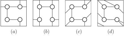
Figure 18: Non-planar graphs for $k=3$.

After assigning labels to the vertices and lengths to the bridges compatible with the operators’ $R$-charges, one generates $32$ distinct configurations as indicated in the corresponding entry of Table 7. Regardless of the assignments, the graphs $(a),\,(b)$ and $(d)$ of Figure 18 produce a vanishing contribution. The vanishing of the cases $(a)$ and $(b)$ can be anticipated only by successive use of the pinching limit of the polygon as illustrated in the expression (3.21). For example, consider the case $(a)$ and label the vertices from 1 to 4 in a clockwise order starting from the top left operator. There is a single face corresponding to an icosagon ($20$-gon) bounded by the bridges. Taking into account the order of the vertices along this boundary, we have the one-loop contribution given by $\mathop{\texttt{polygon}}(1,2,1,3,4,2,1,2,4,3)$. We now apply several pinching limits to reduce that sequence down to $\mathop{\texttt{polygon}}(1,3)$ which would correspond to a two-point function, and that is zero by supersymmetry.

The graph $(d)$ is decomposed into a hexagon and an octadecagon, and both vanish once we use the corresponding one-loop expression as given in (3.15).

The only non-trivial graph is $(c)$, which produces a non-zero result. However, after summing over all labelings, those contributions simply cancel out. Therefore, the non-planar graphs do not contribute, and once again we expect to obtain the final result simply from the stratification contribution (5.56), which reads in this case

$$\langle\mathcal{Q}^{3}_{1}\mathcal{Q}^{3}_{2}\mathcal{Q}^{3}_{3}\mathcal{Q}^{3}_{4}\rangle^{1-\text{loop}}_{(g=1)}=\frac{18g^{2}}{N_{\text{c}}^{4}}(X+Y+Z)\,R\,F^{(1)}(z)\,.$$ (6.5)

For comparison with perturbative data, we now consider the case $Z=0$. We find that for the two cases considered here:

$$\langle\mathcal{Q}^{k}_{1}\mathcal{Q}^{k}_{2}\mathcal{Q}^{k}_{3}\mathcal{Q}^{k}_{4}\rangle^{1-\text{loop}}_{(g=1)}\xrightarrow{\;Z=0\;}-\frac{1}{N_{\text{c}}^{2}}G_{k,(g=0)}^{\text{1-loop}}\quad\text{for}\quad k=2,3\,.$$ (6.6)

and this perfectly matches with the data shown in Table 5.

6.1.2 $k=4$

The case $k=4$ is significantly more involved than the previous ones. The number of non-planar graphs is $57$, and they give $441$ distinct physical configurations when operator labelings and bridge lengths are chosen.

Let us consider one example in detail. Among the 441 graphs with assigned labels and bridge lengths, we have the following example

$$\parbox[c]{43.362pt}{\includegraphics{FigTorusExamplek4}}\;,$$ (6.7)

where each solid line now corresponds to a propagator. This graph is decomposed into two polygons: An octagon (dark gray) and a hexadecagon (light gray). Accounting for the corresponding propagators, we have that this contribution is given by

$$\frac{X^{2}Y^{2}}{N_{\text{c}}^{4}}\bigl{(}\mathop{\texttt{polygon}}(1,2,4,3)+\mathop{\texttt{polygon}}(1,2,4,3,1,3,4,3)\bigr{)}\,.$$ (6.8)

We can now simply use the expression for the corresponding polygon using (3.15) to get the final result. Alternatively, we observe that using the pinching limit, the hexadecagon degenerates into an octagon as follows,

$$\mathop{\texttt{polygon}}(1,2,4,{\color[rgb]{1,0,0}3},1,{\color[rgb]{1,0,0}3},4,3)\rightarrow\mathop{\texttt{polygon}}(1,2,4,{\color[rgb]{0,0,1}3},4,{\color[rgb]{0,0,1}3})\rightarrow\mathop{\texttt{polygon}}(1,2,4,3)\,.$$ (6.9)

Now plugging in the corresponding expression for the one-loop octagon from (5.55), we get that this graph produces

$$-\frac{g^{2}}{N_{\text{c}}^{4}}XY\left(X^{2}z\bar{z}+Y^{2}+XY(z\bar{z}-2z-2\bar{z}+1)+Z(X+Y)(z+\bar{z}-z\bar{z}-1)\right)F^{(1)}(z)\,.$$ (6.10)

All other graphs are equally straightforward to compute as this example. Upon summing over the 441 graphs and adding the stratification contribution (5.56), we recover the prefactor $R$ and the final result is given by

$$\langle\mathcal{Q}^{4}_{1}\mathcal{Q}^{4}_{2}\mathcal{Q}^{4}_{3}\mathcal{Q}^{4}_{4}\rangle^{1-\text{loop}}_{(g=1)}=-\frac{32g^{2}}{N_{\text{c}}^{4}}\left(5\,(X^{2}+Y^{2}+Z^{2})+12\,(XY+XZ+YZ)\right)\,R\,F^{(1)}\,.$$ (6.11)

After setting $Z=0$ and comparing with the data of Table 5 for $k=4$, we find again a perfect agreement.

6.1.3 $k=5$

We have extended our analysis to the case $k=5$, which involves $2760$ distinct graphs. The procedure is no different from the previous cases, and we simply display here the result from the summation over all those genus-one graphs, together with the stratification contribution. Once again, we recover the universal prefactor $R$ (5.57) and the outcome reads

$$\langle\mathcal{Q}^{5}_{1}\mathcal{Q}^{5}_{2}\mathcal{Q}^{5}_{3}\mathcal{Q}^{5}_{4}\rangle^{1-\text{loop}}_{(g=1)}= -\frac{50g^{2}}{N_{\text{c}}^{4}}\Bigl{(}108\,XYZ+23\left(X^{3}+Y^{3}+Z^{3}\right)$$ (6.12)

$$+51\left(X^{2}Y+X^{2}Z+XY^{2}+XZ^{2}+Y^{2}Z+YZ^{2}\right)\Bigr{)}\,R\,F^{(1)}\,.$$

When $Z=0$ we again recover the perturbative result of Table 5.

To summarize the findings of this section: By summing over genus-one graphs and adding the stratification contribution determined in Section 5, we computed the four-point correlator for a generic polarization of the external BPS operators. We compared these results with data for the particular polarization studied in literature, namely when $Z=0$, and found a perfect match in all cases, which strongly corroborates our proposal. The $Z\neq 0$ results are simple predictions of the hexagonalization procedure, which would be nice to check against a direct perturbative computation.

6.2 Checks at Large $k$

6.2.1 $k\gg 1$: Leading Order

Another interesting case that we will focus on in the following are contributions $\mathcal{F}_{k,m}$ where both $m$ and $(k-m)$ are large, that is we look at the limit $k\gg 1$ with $0<m/k<1$. In this regime, the four operators are connected by a parametrically large number $\mathcal{O}(k)$ of propagators. This implies that graphs where the propagators connecting any two operators are distributed on as many bridges as possible outweigh all other graphs by combinatorial factors. In other words, graphs where any bridge is only filled with a few (or zero) propagators are suppressed by powers of $1/k$. Namely, the sum over distributions of $n$ propagators on $j$ bridges at large $n$ expands to

$$\sum_{\begin{subarray}{c}n_{0}\leq n_{1},\dots,n_{j}\leq n\\ \sum_{i}n_{i}=n\end{subarray}}1=\frac{n^{j-1}}{(j-1)!}+\frac{j(1-2n_{0})n^{j-2}}{2(j-2)!}+\mathcal{O}(n^{j-3})\,,\quad j\in\mathbb{Z}_{>0}\,.$$ (6.13)

This combinatorial dominance greatly reduces the number of contributing graphs: For a correlator with generic polarizations $\alpha_{i}$, only the maximal graphs 1.1, 2.1.1–2.1.3, 3.1, and 3.2 of Table 1 contribute to the leading order in $1/k$, since all other graphs have fewer bridges. For these graphs, every face has room for exactly one hexagon, and thus all mirror magnons live on bridges with a large number $\mathcal{O}(k)$ of propagators, which means that all quantum corrections are delayed. However, in this work, we consider operator polarizations with $(\alpha_{1}\cdot\alpha_{4})=(\alpha_{2}\cdot\alpha_{3})=0$, which do not admit propagator structures of the type $Z\equiv(\alpha_{1}\cdot\alpha_{4})(\alpha_{2}\cdot\alpha_{3})/x_{14}^{2}x_{23}^{2}$, see (4.2). In other words, there are no contractions between operators $1$ and $4$, and no contractions between operators $2$ and $3$. Hence, even at large $k$, the dominant graphs will leave room for zero-length bridges and thus admit quantum corrections already at one-loop order.

Before diving into the computation, let us quote the leading and first subleading terms in $1/k$ of our data from Table 5 for reference (subleading terms are shown in gray):

$$\mathcal{F}_{k,m}^{(1),\mathrm{U}}(z,\bar{z})\big{|}_{\text{torus}} =$$

$$\mspace{-110.0mu}-\frac{2k^{2}}{N_{\text{c}}^{4}}\biggl{\{}\Bigl{(}\bigl{[}{\textstyle\frac{17r^{4}}{6}}-{\textstyle\frac{7r^{2}}{4}}+{\textstyle\frac{11}{32}}\bigr{]}k^{4}{\color[rgb]{.5,.5,.5}\mbox{}+\bigl{[}{\textstyle\frac{9r^{2}}{2}}-{\textstyle\frac{13}{8}}\bigr{]}k^{3}}\Bigr{)}t{\color[rgb]{.5,.5,.5}\mbox{}-r\bigl{[}{\textstyle\frac{34r^{2}}{3}}-{\textstyle\frac{7}{2}}\bigr{]}k^{3}s_{-}+\mathcal{O}(k^{2})}\biggr{\}}{\color[rgb]{1,0,0}F^{(1)}}\,,$$ (6.14)

$$\mathcal{F}_{k,m}^{(2),\mathrm{U}}(z,\bar{z})\big{|}_{\text{torus}} =$$

$$\mspace{-90.0mu}\frac{4k^{2}}{N_{\text{c}}^{4}}\Biggl{[}\biggl{\{}\Bigl{(}\bigl{[}{\textstyle\frac{17r^{4}}{6}}-{\textstyle\frac{7r^{2}}{4}}+{\textstyle\frac{11}{32}}\bigr{]}k^{4}{\color[rgb]{.5,.5,.5}\mbox{}+\bigl{[}{\textstyle\frac{9r^{2}}{2}}-{\textstyle\frac{13}{8}}\bigr{]}k^{3}}\Bigr{)}t{\color[rgb]{.5,.5,.5}\mbox{}-r\bigl{[}{\textstyle\frac{34r^{2}}{3}}-{\textstyle\frac{7}{2}}\bigr{]}k^{3}s_{-}}\biggr{\}}{\color[rgb]{1,0,0}F^{(2)}}$$

$$\mspace{-72.0mu}+\biggl{\{}\Bigl{(}\bigl{[}{\textstyle\frac{29r^{4}}{24}}-{\textstyle\frac{11r^{2}}{16}}+{\textstyle\frac{15}{128}}\bigr{]}k^{4}{\color[rgb]{.5,.5,.5}\mbox{}+\bigl{[}{\textstyle\frac{17r^{2}}{8}}-{\textstyle\frac{21}{32}}\bigr{]}k^{3}}\Bigr{)}t^{2}{\color[rgb]{.5,.5,.5}\mbox{}-r\bigl{[}{\textstyle\frac{23r^{2}}{3}}-{\textstyle\frac{9r}{4}}\bigr{]}k^{3}ts_{-}}\biggr{\}}{\color[rgb]{1,0,0}\bigl{(}F^{(1)}\bigr{)}^{2}}$$

$$\mspace{-72.0mu}{\color[rgb]{.5,.5,.5}\mbox{}-\bigl{[}{\textstyle\frac{5r^{2}}{4}}-{\textstyle\frac{19}{48}}\bigr{]}k^{3}{\color[rgb]{1,0,0}F^{(2)}_{\mathrm{C,+}}}+\mathcal{O}(k^{2})}\Biggr{]}\,.$$ (6.15)

Polygonization: Maximal Cyclic Graphs.

Since there are no contractions between operators $1$ and $4$ and between operators $2$ and $3$, we need to consider graphs where the four operators are cyclically connected, as in $1$—$2$—$4$—$3$—$1$ (later we will see that non-cyclic graphs are also important). We can obtain all possible graphs of this type by deleting bridges from the maximal graphs listed in Table 1. Among all cyclically connected graphs, we only consider graphs where as many bridges as possible are filled. We will call those “maximal cyclic graphs”. These will be the only graphs that contribute at leading order in $1/k$. All further graphs only contribute to subleading orders in $1/k$, and can be obtained by setting further bridge lengths to zero.

Starting from any of the $16$ cases listed in Table 1, we can obtain cyclic graphs by grouping the four operators into two pairs and deleting all bridges that connect the members of either pair. Doing this in all possible ways for all the $16$ graphs, and discarding non-maximal as well as duplicate graphs, we end up with the complete set of maximal cyclic graphs A through Q displayed in Table 8.

A	B	C	D
E	F	G	H
I	J	K	L
M	N	P	Q

Table 8: Inequivalent maximal cyclic graphs on the torus.

For example, consider the maximal graph 1.1. We can delete either all vertical or all horizontal lines; these two cases are equivalent and give

$$\parbox[c]{43.362pt}{\includegraphics{FigTorusCase11}}\;\rightarrow\;\parbox[c]{43.362pt}{\includegraphics{FigTorusCase11A}}\;,$$ (6.24)

which is easily recognized as case A. Alternatively, we could delete all diagonal lines, which gives case P. In fact, for all cases 1.1–1.5.3 we do not need to consider deleting the diagonal lines, as the resulting configurations will (by construction) always be covered by the cases 2.1.1–3.2. Moving on to cases 1.2.1 and 1.2.2, up to operator relabelings, all ways of deleting bridges (keeping the diagonal ones) lead to equivalent configurations:

$$\parbox[c]{43.362pt}{\includegraphics{FigTorusCase121}}\;,\;\parbox[c]{43.362pt}{\includegraphics{FigTorusCase122}}\quad\rightarrow\quad\parbox[c]{43.362pt}{\includegraphics{FigTorusCase121B}}\;,$$ (6.25)

which we recognize as case B. The derivation of the further cases C through Q from the maximal graphs in Table 1 is listed in Appendix B.2.

The large-weight limit brings about another simplification: In Section 6.1 above, we saw that magnons carrying non-trivial R-charges may cancel $Z$ propagator structures (4.1) such that the final result is free of $Z$’s. Such cancellations cannot occur here, since all graphs of Table 8 dissect the torus into four octagons separated by large bridges. Such octagons do not leave enough room for $Z$ propagator cancellations. Hence we do not have to include graphs containing $Z$ propagators.

Looking at the cases A through Q, we find that the bridge configurations of the cases A, C, D, E, F, H, I, J, N, and K imply a constraint on $m$: Either $m=0$, or $m=k$. Hence, even though no further bridges can be added to these graphs (under the cyclicity constraint), these cases are suppressed at large $m$ and $(k-m)$, and only the cases B, G, L, M, P, and Q remain (these were called B, A, C, D, E, and F in our previous publication [1]). For these graphs, we now have to consider all possible operator labelings, taking care that some seemingly different labelings in fact produce identical bridge configurations. In addition, each labeled graph comes with a combinatorial factor from the distribution of propagators on the various bridges according to (6.13). We list all inequivalent labelings for the relevant graphs as well as their combinatorial factors in Table 9.

Case	Inequivalent Labelings	Combinatorial Factor
B	$(1,2,4,3),(2,1,3,4),(3,4,2,1),(4,3,1,2)$	$m^{3}(k-m)/6$
B	$(1,3,4,2),(3,1,2,4),(2,4,3,1),(4,2,1,3)$	$m(k-m)^{3}/6$
G	$(1,2,4,3),(3,4,2,1)$	$m^{4}/24$
G	$(1,3,4,2),(2,4,3,1)$	$(k-m)^{4}/24$
L	$(1,2,4,3),(3,4,2,1),(2,1,3,4),(4,3,1,2)$	$m^{2}/2\cdot(k-m)^{2}/2$
M	$(1,2,4,3),(2,1,3,4),(1,3,4,2),(3,1,2,4)$	$m^{2}(k-m)^{2}/2$
P	$(1,2,4,3)$	$m^{2}(k-m)^{2}/2$
Q	$(1,2,4,3)$	$m^{2}(k-m)^{2}$

Table 9: All inequivalent operator labelings for the graphs that contribute to leading order in $1/k$, together with their combinatorial factors according to (6.13). The order of the labels runs clockwise, starting at the top left operator in the graphs of Table 8.

For case P, all operator labelings are equivalent. Beyond that, it has an extra symmetry: Every pair of operators is connected by a pair of bridges. Exchanging the members of all pairs simultaneously amounts to a cyclic rotation of the four operators and thus leaves the configuration invariant. This operation is an example of a graph automorphism, see the last part of Section 2.2, in particular (2.17). The naive sum over bridge lengths gives a combinatorial factor $m^{2}(k-m)^{2}$, which thus has to be corrected by a factor of $1/2$.

Sprinkling: One and Two Loop Check.

The previous maximal cyclic graphs polygonalize the torus into four octagons each, generating some toroidal polyhedra. We represent their corresponding nets in Table 10 for easier visualization. The one-loop and two-loop computations can then be performed straightforwardly from a single particle sitting in the single ZLB of each octagon. Such contributions can be easily computed to any desired loop order using the ingredients of Appendix D (at one loop we can simply use the $\mathop{\texttt{polygon}}$ function of Section 3.1). At one loop this is the only particle configuration contributing. At two loops, we have to consider in addition two virtual particles in different octagons, which essentially amounts to the one-loop octagon squared. The contribution of two virtual particles inserted in the same octagon turns out to be delayed to four loops as shown in Appendix D. The final step is then to sum over the labelings of the vertices, weighted by the combinatorial factors arising from the different ways of distributing the propagators among the bridges. Table 9 contains the details of these combinatorics. We have performed this calculation in [1] and found a perfect agreement with the large $k$ data (6.14) and (6.15).

Case	Hexagonalization	Case	Hexagonalization
B		G
L		M
P		Q

Table 10: After completing the relevant skeleton graphs B, G, L, M, P, and Q with the missing ZLBs, we obtain complete hexagonalizations of the four-punctured torus. The outcome is that each configuration is decomposable into $8$ hexagons, or $4$ minimal octagons, using the terminology of Section 3.1. The distinct octagons are colored in white and gray. The colored edges correspond to the physical ones, with the operators being labeled as A, B, C, and D. The subscript in each edge label indicates to which of the eight hexagons the respective edge belongs. Later on, we will specify the labels A, B, C, and D of the operators. For each hexagonalization, the dashed lines correspond to the ZLBs, while the solid gray bridges have non-zero lengths.

Sprinkling: Three Loop Prediction.

As far as we know, there is no available non-planar perturbative data at three loops. The planar case, however, was computed in [46]. Here, we are going to make a prediction for the three-loop result at leading order in large $k$ using integrability. In principle, one can keep going and make predictions for arbitrary order in $g^{2}$, and it would be very interesting to try to re-sum the series. At three loops, one has the following possible contributions:

1. Three-loop correction of the one-particle octagon.

2. Two mirror particles inserted at different octagons.

3. Three mirror particles inserted at three different octagons.

4. Multiple mirror particles inserted in the same octagon.

One can show that contribution 3 is only present for case P, because all other cases only have two octagons involving four operators, and an octagon involving only three (or two) operators vanishes as the relevant cross-ratio for gluing is either $0$, $1$, or $\infty$. The contribution 4 kicks in only at four loops – the case of two mirror particle in the same edge is computed in the Appendix D – and thus is not relevant here.

The new ingredient for the three-loop computation, when compared to the two-loop calculation performed in [1], is the one-particle mirror contribution in a ZLB expanded to three loops, given by (see Appendix D for details):

$$\mathcal{M}^{(1)}(z)=\left(z+\bar{z}-\frac{\alpha+\bar{\alpha}}{2}\left(1+\frac{z\bar{z}}{\alpha\bar{\alpha}}\right)\right)\times\\ \times\bigl{(}g^{2}F^{(1)}(z,\bar{z})-2g^{4}F^{(2)}(z,\bar{z})+6g^{6}F^{(3)}(z,\bar{z})+\mathcal{O}(g^{8})\bigr{)}\,,$$ (6.47)

where $F^{(3)}$ is the three-loop ladder integral defined as

$$F^{(3)}(z,\bar{z})=\frac{x_{13}^{2}x^{2}_{24}x^{4}_{14}}{\pi^{6}}\int\frac{d^{4}x_{5}d^{4}x_{6}d^{4}x_{7}}{x_{15}^{2}x_{45}^{2}x^{2}_{35}x^{2}_{56}x^{2}_{16}x^{2}_{46}x^{2}_{67}x^{2}_{17}x^{2}_{47}x^{2}_{27}}\,=\,\parbox[c]{52.0344pt}{\includegraphics{FigTripleBoxInt}}\,.$$ (6.48)

The one-loop and two-loop ladder integrals $F^{(1)}$ and $F^{(2)}$ are defined in (4.4) and (4.5) (see also the expression (D.32) in terms of polylogarithms), and the cross ratios $z$, $\bar{z}$ are defined in (3.3).

Using the hexagonalized graphs of Table 10, the combinatorial factors of Table 9, and adding all mirror particle corrections, one arrives at the three-loop prediction

$$\mathcal{F}_{k,m}^{(3),\mathrm{U}}(z,\bar{z})\big{|}_{\text{torus}}= -\frac{12k^{2}}{N_{\text{c}}^{4}}\Biggl{[}\biggl{\{}\Bigl{(}\bigl{[}{\textstyle\frac{17r^{4}}{6}}-{\textstyle\frac{7r^{2}}{4}}+{\textstyle\frac{11}{32}}\bigr{]}k^{4}\Bigr{)}t{\color[rgb]{.5,.5,.5}\mbox{}+\mathcal{O}(k^{3})}\biggr{\}}{\color[rgb]{1,0,0}F^{(3)}}$$

$$+\biggl{\{}\Bigl{(}\bigl{[}{\textstyle\frac{29r^{4}}{18}}-{\textstyle\frac{11r^{2}}{12}}+{\textstyle\frac{5}{32}}\bigr{]}k^{4}\Bigr{)}t^{2}{\color[rgb]{.5,.5,.5}\mbox{}+\mathcal{O}(k^{3})}\biggr{\}}{\color[rgb]{1,0,0}F^{(2)}F^{(1)}}$$

$$+\biggl{\{}\Bigl{(}\bigl{[}{\textstyle\frac{(1-4r^{2})^{2}}{96}}\bigr{]}k^{4}\Bigr{)}t^{3}{\color[rgb]{.5,.5,.5}\mbox{}+\mathcal{O}(k^{3})}\biggr{\}}{\color[rgb]{1,0,0}\bigl{(}F^{(1)}\bigr{)}^{3}}\Biggr{]}\,.$$ (6.49)

6.2.2 $k\gg 1$: Subleading Order

Next, we are going to compute the subleading contribution in the large-$k$ expansion, i. e. the terms of order $\mathcal{O}(k^{3})$, at one-loop order using integrability. We find an agreement with the perturbative data (gray) given in (6.14). As described in detail below, the subleading computation receives contributions from three different sources: The graphs used in the leading-order computation, the graphs obtained from the leading-order graphs by deleting one bridge, and the “deformed” graphs which are graphs having one pair of propagators of type $Z$.

Leading Cyclic Graphs.

The graphs B, G, L, M, P, and Q used in the leading-order computation also contribute at subleading order in large $k$. The integrability contribution is computed exactly as in the leading-order case, in particular one uses the same set of hexagons of Table 10, however one considers the subleading contribution to the combinatorial factors given in (6.13), with $n_{0}=1$. Recall that to obtain a final term with the propagator structure $X^{m}Y^{k-m}$ at one-loop order, it is necessary to consider also the neighboring tree-level graphs with propagators $X^{m-1}Y^{k-m+1}$ and $X^{m+1}Y^{k-m-1}$. This follows because the mirror particles carry $R$-charge and they can change the propagator structure of a tree-level graph [1], which is seen explicitly by the ratios of $X$, $Y$, and $Z$ propagator factors in the prefactor of (6.47) rewritten via (5.54):

$$\left(z+\bar{z}-\frac{\alpha+\bar{\alpha}}{2}\left(1+\frac{z\bar{z}}{\alpha\bar{\alpha}}\right)\right)\\ =\frac{1}{2}\biggl{[}1-\frac{Y}{X}+z\bar{z}\left(1-\frac{X}{Y}\right)+(1-z)(1-\bar{z})\left(\frac{Z}{X}+\frac{Z}{Y}-2\right)\biggr{]}\,.$$ (6.52)

One important remark is that, differently from the leading case, where the combinatorial factor of each graph is universal, in the subleading case the combinatorial factor changes when considering the neighboring graphs. As an example, Table 11 shows the combinatorial factors relevant for case B.

Tree-Level Propagators	Labelings: (1,2,4,3), (2,1,3,4), (3,4,2,1), (4,3,1,2).	Labelings: (1,3,4,2), (3,1,2,4), (2,4,3,1), (4,2,1,3).
$X^{m}Y^{k-m}$	$-(k-m)m^{2}-\frac{m^{3}}{6}$	$-\frac{1}{6}(k-m)^{3}-(k-m)^{2}m$
$X^{m-1}Y^{k-m+1}$	$-\frac{3}{2}(k-m)m^{2}$	$-\frac{3}{2}(k-m)^{2}m$
$X^{m+1}Y^{k-m-1}$	$-\frac{1}{2}(k-m)m^{2}-\frac{m^{3}}{3}$	$-\frac{1}{3}(k-m)^{3}-\frac{1}{2}(k-m)^{2}m$

Table 11: The combinatorial factors used for the subleading computation of the graph B. The case B has eight inequivalent labelings, see Table 9.

Subleading Cyclic Graphs.

In addition to the leading-order graphs, there will be contributions from cyclic graphs that are obtained from the cases B, G, L, M, P, and Q by removing one of their bridges. Deleting a bridge in all possible ways, and identifying identical graphs, we find seven inequivalent subleading cyclic graphs, see Table 12. The number of inequivalent labelings is indicated in the parentheses below each graph. The hexagonalization of the subleading cyclic graphs can be obtained from the hexagonalization of the leading cyclic graphs given previously by replacing the corresponding line that was deleted in the process by a zero-length bridge. The final step is to add the mirror particles. In this case, we have one-, two- and three-particle contributions, because there are four hexagons sharing bridges of zero length in a sequence. Thus at one-loop order for the integrability computation, one uses the expressions for both the octagon and the dodecagon of (3.15). In addition, the relevant combinatorial factors can be read from the leading term of formula (6.13).

B.1 (8)	G.1 (4)	L.1 (8)	L.2 (8)
L.3 (8)	P.1 (4)	Q.1 (4)

Table 12: The seven inequivalent graphs that are obtained by deleting one bridge from graphs B, G, L, M, P, or Q of Table 8. These graphs contribute at subleading order in $k$. The parentheses show the number of inequivalent labelings that each graph has.

Deformed Graphs.

At subleading order in large $k$, there is room for so-called deformed graphs. The mirror particles carry $R$-charge, in other words they depend on the $R$-charge cross ratios $\alpha$ and $\bar{\alpha}$, as seen for example in (6.52). Hence the final $R$-charge structure of a graph depends not only on the tree-level propagators, but also on the mirror particles. For example, graphs that include a propagator of the type $Z\equiv(\alpha_{1}\cdot\alpha_{4})(\alpha_{2}\cdot\alpha_{3})/x_{14}^{2}x_{23}^{2}$ can give a final term free of $Z$’s after the inclusion of the mirror corrections, which is thus compatible with our chosen polarizations (4.2), and gives a non-zero contribution in the limit $Z\rightarrow 0$. We have already encountered the same phenomenon when we performed checks for finite $k$. In the sum over graphs, we hence must include graphs with $Z$ propagators.

Graphs containing one or more propagators of type $Z$ (and otherwise only large bridges filled with many propagators) will be called deformed graphs. At one loop, the relevant deformed graphs include only one pair of $Z$ propagators connecting two disjoint pairs of operators. We can classify all such graphs by starting with the set of maximal graphs listed in Table 1, declaring two of the bridges to become $Z$ propagators, and deleting other bridges such that the graph becomes subleading in $k$. In the limit of large $k$ that we consider, extremal graphs with $m=0$ or $(k-m)=0$ will not contribute. Taking into account that one of the bridges attaching to each operator in Table 1 will become a $Z$ propagator, this means that we only need to consider the graphs 1.2.1, 1.2.2, 1.5.3, 2.1.1, 2.1.2, 2.1.3, 3.1, and 3.2. Starting with these, and deleting bridges / replacing bridges by $Z$ propagators, we arrive at the set of inequivalent deformed graphs shown in Table 13.

1.2.1A (8)	1.2.1B (8)	1.2.1C (8)	1.2.2A (8)	1.2.2B (8)
1.5.3A (4)	1.5.3B (4)	2.1.1A ($6\cdot 8$)	2.1.1B ($6\cdot 8$)	2.1.1C ($6\cdot 8$)
2.1.2A (8)	2.1.2C (8)	2.1.3A (8)	2.1.3B (8)
3.1A (${\color[rgb]{0,0.6,0}2{\cdot}4},{\color[rgb]{0,0,1}8}$)	3.1B (${\color[rgb]{0,0,1}2{\cdot}8}$)	3.1C (${\color[rgb]{0,0.6,0}2{\cdot}4},{\color[rgb]{0,0,1}8}$)	3.1D (${\color[rgb]{0,0.6,0}3{\cdot}4},{\color[rgb]{0,0,1}2{\cdot}8}$)

Table 13: All inequivalent deformed graphs that contribute to the first subleading order in $1/k$. Wiggly lines stand for $Z$ propagators. Graphs with crossed bridges stand for classes of graphs where any one of the crossed bridges is deleted. The parentheses show the number of inequivalent labelings. Recall that for the hexagonal graphs, opposite edges of the outer hexagon are identified.

Alternatively, the graphs in Table 13 can be obtained by starting with the graphs B, G, L, M, P, and Q of Table 8, and inserting $Z$ propagators as well as deleting one bridge in all possible ways.

After having determined all deformed graphs, the next step is the hexagonalization. This is done by adding bridges of zero length to the graphs, and dividing them into eight hexagons. Due to the flip invariance of the mirror particle corrections, any different set of zero-length bridges will give the same final result. In the case of the deformed graphs, the multi-particle contribution will show up, and we use the expression for the octagon, decagon, and dodecagon of (3.15). In order to perform the integrability computation for the deformed graphs, one uses that $\alpha$ and $\bar{\alpha}$ are determined by the equations (5.54). The limit $Z\rightarrow 0$ is only taken after adding the mirror-particle corrections to a graph. Similar to the case of the leading cyclic graphs, to get a final term proportional to $X^{m}Y^{k-m}$ at one-loop, one has to consider the set of graphs corresponding to the tree-level terms $X^{m-1}Y^{k-m}Z$ and $X^{m}Y^{k-m-1}Z$. Most of the graphs of Table 13 give a vanishing contribution. One example of a non-vanishing graph is

$$\text{Case}\;1.2.1\mathrm{C} =\sum_{s=0}^{1}\frac{4}{6}\left(m^{3}\mathcal{M}^{(1)}(1-z)+(k-m)^{3}\mathcal{M}^{(1)}\left(\frac{z}{z-1}\right)\right)X^{m-s}\,Y^{k-m-1+s}\,Z$$

$$\xrightarrow{\;Z\to 0\;}\,\frac{1}{3}\left(k^{3}-3k^{2}m+3km^{2}-2m^{3}\right)(z\bar{z}-1)F^{(1)}(z,\bar{z})\,X^{m}Y^{k-m}\,.$$ (6.75)

Summary.

The subleading integrability result is obtained by summing three different kinds of contributions which were described above. The final result agrees with the perturbative data. It is possible to use the same steps to compute the predictions for the remaining orders in $k$.

7 Conclusions

We performed detailed tests of our proposal on the application of the hexagon formalism to non-planar correlators at weak coupling. The basic strategy is the same as in the planar case; we first draw all possible tree-level diagrams on a given Riemann surface, dissect them into hexagonal patches, and glue those patches back together by summing over complete sets of intermediate (mirror) states. The key new idea that is essential in the non-planar case is the procedure called stratification: We first computed all contributions coming from tree-level graphs drawn on a torus, including the graphs that are actually planar. After doing so, we subtracted the contributions from degenerate Riemann surfaces, which in turn can be computed by taking the planar results and shifting the rank of the gauge group. The procedure was tested against available perturbative data, and the results agree perfectly.

What we developed in this paper may be viewed as a bottom-up approach to construct a new way of performing string perturbation theory, based on the triangulation of the worldsheet. The central object in our formalism is the hexagon, which is a branch-point twist operator on the worldsheet. The idea of using the twist operator for constructing higher-genus surfaces is not new; it was one of the motivations for Knizhnik to conduct detailed studies of twist operators [47]. It also showed up in other important contexts such as the low-energy description of matrix string theory [48, 49]. In this sense, the hexagon formalism is yet another instance of “old wine in new bottles”, which we have been encountering multiple times in recent years.

There are several obvious next steps. It would be important to extend the computation to higher loops, both in $\lambda$ and in $1/N_{\text{c}}$. Also desirable would be to tie up several loose ends in our arguments: For instance, in the discussion in Section 5, we estimated the contribution from certain magnon configurations (5.45) by claiming that they are related to simpler configurations via Dehn twists and flip transformations. It would be nice to perform a direct computation of such configurations and show the flip invariance explicitly.

One practical obstacle for doing such computations is the complexity of the multi-particle integrands. Even for the two- and three-magnon contributions at one loop which were studied in this paper, the integrands are horrendously complicated. Given the simplicity of the final answer, it would be worth trying to find a better way to organize the integrand. This will eventually be crucial if we were to perform more complicated and physically interesting computations, such as taking the strong-coupling limit and reproducing the supergravity answers. Another strategy is to avoid dealing with the complicated integrand for now, and look for simplifying limits. In flat space, it was shown by Gross and Mende that the high-energy string scattering takes a remarkably simple and universal form [50, 51]. The results were later used by Mende and Ooguri, who succeeded in Borel-resumming the higher-genus contributions in the same limit [52]. In our context, the analogue of the high-energy limit would be played by large operator lengths (charges). As already observed in this paper, taking the large-charge limit simplifies the computation drastically. It is therefore interesting to analyze the limit in more detail, and possibly try to re-sum the $1/N_{\text{c}}$ corrections [33, 34]. It would be even more exciting if we could make a quantitative prediction for the non-perturbative corrections by analyzing the large-order behavior of the $1/N_{\text{c}}$ expansion [53], which one could test against the direct instanton computation [54, 55, 56, 57].

The relation between the summation over graphs and the integration over the moduli space of Riemann surfaces deserves further study. As mentioned in the introduction, one big puzzle in this regard is the fact that the summation over graphs is discrete, while the moduli space is continuous. In the study of simple matrix models, such a discretization of the moduli space was attributed to the topological nature of the dual worldsheet theory. We should however note that the discretization could take place even in non-topological worldsheet theories, namely in the light-cone quantization of the DLCQ background [48, 49, 58]. This is in fact closer to our context since, in the generalized light-cone gauge, the lengths of the string becomes proportional to the angular momentum in $\mathrm{S}^{5}$, which takes discrete values. To make more progress on these points, it would perhaps be helpful to study the recently proposed worldsheet action for the DLCQ background [59], which is suited for quantization in the conformal gauge, and clarify how the conformal-gauge computation reproduces the light-cone gauge expectation that the moduli space gets discretized.

As a final remark, let us emphasize that the results in this paper are just the first steps in the application of integrability to non-planar observables: Firstly, it would also be interesting to understand other non-planar quantities, such as non-planar anomalous dimensions of single-trace operators, and anomalous dimensions of double-trace operators. See [13] for an important initial attempt. Secondly, although it is remarkable that integrability can reproduce non-planar quantities, the computation performed in this paper is almost as complicated as the direct perturbative computation, and as we include more and more mirror particles, we face the integrand challenges alluded to above. Is there something better we can do? Can we reformulate this formalism, for instance, by combining it with the quantum spectral curve [61]? In fact, there are already two data points which indicate that the quantum spectral curve could be useful for analyzing correlation functions [62, 63]. Whatever the upgraded formalism will be, we expect that the results in this paper will be useful in finding it.

Acknowledgments

We would like to thank Benjamin Basso, Nathan Berkovits, Niklas Beisert, Vasco Gonçalves, Frank Coronado, Vladimir Kazakov, Gregory Korchemsky, Juan Maldacena, Tristan McLoughlin, and Soo-Jong Rey for discussions. We also thank Vasco Gonçalves for helping us with the expansion of the mirror bound-state $S$-matrix elements. TB would like to thank DESY Hamburg for its support and hospitality during all stages of this work, Perimeter Institute for two very fruitful visits, and KITP Santa Barbara for an extended stay while this project was carried out. TF would like to thank the warm hospitality of the Laboratoire de Physique Théorique de l’Ecole Normale Supérieure and Nordita, where part of this work was done. TF would like to thank also CAPES/INCTMAT process 88887.143256/2017-00 for financial support. The work of JC and TF was supported by the People Programme (Marie Curie Actions) of the European Union’s Seventh Framework Programme FP7/2007-2013/ under REA Grant Agreement No 317089 (GATIS), by the European Research Council (Programme “Ideas” ERC-2012-AdG 320769 AdS-CFT-solvable), from the ANR grant StrongInt (BLANC-SIMI-4-2011). The work of SK was supported by DOE grant number DE-SC0009988. This research was supported in part by the National Science Foundation under Grant No. NSF PHY17-48958. This research was supported in part by Perimeter Institute for Theoretical Physics. Research at Perimeter Institute is supported by the Government of Canada through the Department of Innovation, Science and Economic Development and by the Province of Ontario through the Ministry of Research and Innovation.

Appendix A Details on Non-Planar Data

In (4.10)–(4.12), we represented the quantum corrections $\mathcal{F}_{k,m}$ (4.3) to the four-point correlator $G_{k}$ (4.2) in terms of the conformal box (4.4) and double-box functions (4.5), as well as color factors $C^{1}_{k,m}$ and $C^{i}_{k,m}$, $i\in\{\mathrm{a,b,c,d}\}$. In the following, we will explain the color factors and their evaluation in more detail. We will also give further expressions for $\mathcal{F}_{k,m}$ as well as $\mathcal{\widetilde{F}}_{k,m}$. The expressions depend on the choice of gauge group, and we will present results for both $\mathrm{U}(N_{\text{c}})$ and $\mathrm{SU}(N_{\text{c}})$.

Color Factors.

The color factors $C^{i}_{k,m}$ consist of color contractions of four symmetrized traces from the four operators, dressed with insertions of gauge group structure constants $f_{ab}{}^{c}$. The one-loop color factor reads [43]:

$$C^{1}_{k,m}=\frac{f_{pqe}f_{rs}{}^{e}}{(m+1)!^{2}(k-m-2)!^{2}}\operatorname{tr}((a_{1}\dots a_{k-1}p))\operatorname{tr}((a_{1}\dots a_{m+1}c_{m+2}\dots c_{k-1}s))\\ \times\operatorname{tr}((a_{m+2}\dots a_{k-1}c_{1}\dots c_{m+1}q))\operatorname{tr}((c_{1}\dots c_{k-1}r))\,,$$ (A.3)

and the two-loop color factors are [44]:

$$C^{\text{a}}_{k,m}= \frac{f_{abe}f_{cd}{}^{e}f_{pqt}f_{rs}{}^{t}}{2m!^{2}(k-m-1)!(k-m-3)!}$$

$$\times\operatorname{tr}((d_{1}\dots d_{k-m-1}a_{1}\dots a_{m}a))\operatorname{tr}((a_{1}\dots a_{m}b_{1}\dots b_{k-m-3}bdp))$$

$$\times\operatorname{tr}((d_{1}\dots d_{k-m-1}c_{1}\dots c_{m}r))\operatorname{tr}((c_{1}\dots c_{m}b_{1}\dots b_{k-m-3}cqs))\,,$$

$$C^{\text{b}}_{k,m}= \frac{f_{abe}f_{cd}{}^{e}f_{pqt}f_{rs}{}^{t}}{4m!^{2}(k-m-2)!^{2}}$$

$$\times\operatorname{tr}((d_{1}\dots d_{k-m-2}a_{1}\dots a_{m}bp))\operatorname{tr}((a_{1}\dots a_{m}b_{1}\dots b_{k-m-2}cs))$$

$$\times\operatorname{tr}((d_{1}\dots d_{k-m-2}c_{1}\dots c_{m}aq))\operatorname{tr}((c_{1}\dots c_{m}b_{1}\dots b_{k-m-2}dr))\,,$$

$$C^{\text{c}}_{k,m}= \frac{f_{abe}f_{cd}{}^{e}f_{pqt}f_{rs}{}^{t}}{2m!^{2}(k-m-2)!^{2}}$$

$$\times\operatorname{tr}((d_{1}\dots d_{k-m-2}a_{1}\dots a_{m}bd))\operatorname{tr}((a_{1}\dots a_{m}b_{1}\dots b_{k-m-2}ar))$$

$$\times\operatorname{tr}((d_{1}\dots d_{k-m-2}c_{1}\dots c_{m}cp))\operatorname{tr}((c_{1}\dots c_{m}b_{1}\dots b_{k-m-2}qs))\,,$$

$$C^{\text{d}}_{k,m}= \frac{f_{abe}f_{cd}{}^{e}f_{pqt}f_{rs}{}^{t}}{2m!^{2}(k-m-2)!^{2}}$$

$$\times\operatorname{tr}((d_{1}\dots d_{k-m-2}a_{1}\dots a_{m}bp))\operatorname{tr}((a_{1}\dots a_{m}b_{1}\dots b_{k-m-2}as))$$

$$\times\operatorname{tr}((d_{1}\dots d_{k-m-2}c_{1}\dots c_{m}cq))\operatorname{tr}((c_{1}\dots c_{m}b_{1}\dots b_{k-m-2}dr))\,.$$ (A.4)

Here, $\operatorname{tr}((a_{1}\dots a_{k}))\equiv\operatorname{tr}(T^{(a_{1}}\dots T^{a_{k})})$ denotes a totally symmetrized trace of adjoint gauge group generators $T^{a}$, without $1/n!$ prefactor. In the above formulas, $0\leq m\leq k-2$ for $C^{1,\mathrm{b},\mathrm{c},\mathrm{d}}_{k,m}$, and $0\leq m\leq k-3$ for $C^{\text{a}}_{k,m}$, whereas $C^{\text{a}}_{k-2}\equiv 0$. Pictorially, we can represent the color factors as

$$C^{1}_{k,m} =\parbox[c]{36.8577pt}{\includegraphics{FigC1aligned}}\,, \quad C^{\text{a}}_{k,m} =\parbox[c]{44.0847pt}{\includegraphics{FigCaaligned}}\,, \quad C^{\text{b}}_{k,m} =\parbox[c]{46.9755pt}{\includegraphics{FigCbaligned}}\,,$$

$$C^{\text{c}}_{k,m} =\parbox[c]{36.8577pt}{\includegraphics{FigCcaligned}}\,, \quad C^{\text{d}}_{k,m} =\parbox[c]{46.9755pt}{\includegraphics{FigCdaligned}}\,,$$ (A.5)

where the big circles are the operator traces, the dots are structure constants, the thin lines are single color contractions, and the thick lines are multiple color contractions. For $C^{1}$, the horizontal thick lines stand for $(m+1)$ propagators, while the vertical thick lines stand for $(k-m-1)$ propagators. For the two-loop color factors $C^{\text{a}}$, $C^{\text{b}}$, $C^{\text{c}}$, and $C^{\text{d}}$, the horizontal lines stand for $m$ propagators and the vertical lines stand for $(k-m-2)$ propagators.

Expanding the color factors to subleading order in $1/N_{\text{c}}$ (4.14), the leading coefficients (4.15) are straightforwardly computed [43, 44]. The subleading coefficients ${}^{\circ}\kern-1.2ptC$ are much harder to obtain. Their computation is outlined in the following.

Color Algebra.

We will evaluate the color contractions using the fission and fusion rules

$$\operatorname{tr}(T^{a}BT^{a}C)=\gamma\left(\operatorname{tr}(B)\operatorname{tr}(C)-\frac{n}{N_{\text{c}}}\operatorname{tr}(BC)\right)\,,$$ (A.6)

$$\operatorname{tr}(T^{a}B)\operatorname{tr}(T^{a}C)=\gamma\left(\operatorname{tr}(BC)-\frac{n}{N_{\text{c}}}\operatorname{tr}(B)\operatorname{tr}(C)\right)\,,$$ (A.7)

with $n=0$ for gauge group $\mathrm{U}(N_{\text{c}})$, and $n=1$ for gauge group $\mathrm{SU}(N_{\text{c}})$. The gauge group generators $T^{a}$ are normalized via

$$\operatorname{tr}(T^{a}T^{b})=\gamma\,\delta^{ab}\,.$$ (A.8)

The fusion and fission rules follow from the completeness relation

$$(T^{a})^{i}{}_{j}(T^{a})^{k}{}_{l}=\gamma\left(\delta^{i}_{l}\delta^{k}_{j}-\frac{n}{N_{\text{c}}}\delta^{i}_{j}\delta^{k}_{l}\right)\,.$$ (A.9)

We set $\gamma=1$ to match the normalization of [43, 44]. The structure constants are normalized to

$$[T^{a},T^{b}]=if^{ab}{}_{c}\,T^{c}\,,$$ (A.10)

such that

$$f_{abc} =-i\operatorname{tr}([T_{a},T_{b}]T_{c})=-i\operatorname{tr}(T_{a}T_{b}T_{c})+i\operatorname{tr}(T_{c}T_{b}T_{a})\,,$$ (A.11)

$$f_{abe}f_{cd}{}^{e} =-\operatorname{tr}([T_{a},T_{b}][T_{c},T_{d}])$$

$$=-\operatorname{tr}(T_{a}T_{b}T_{d}T_{e})+\operatorname{tr}(T_{a}T_{b}T_{e}T_{d})+\operatorname{tr}(T_{a}T_{d}T_{e}T_{b})-\operatorname{tr}(T_{a}T_{e}T_{d}T_{b})\,.$$ (A.12)

Results of Contractions.

We have explicitly performed the contractions in (A.3) and (A.4) with Mathematica for various different values of $k$ and $m$, for some coefficients up to $k=8$, for others up to $k=9$. The results for the subleading color coefficients are displayed in Table 4 (page 4). Depending on the algorithm, the computation can take very long (up to ${\sim}1$ day on $16$ cores for a single coefficient at fixed $k$ and $m$) and becomes memory intensive (up to ${\sim}100\,$GB) at intermediate stages.

As indicated in the main text, the subleading color coefficients ${}^{\circ}\kern-1.2ptC^{1}_{k,m}$, ${}^{\circ}\kern-1.2ptC^{i}_{k,m}$ have to be polynomials in $k$ and $m$ (up to boundary cases at extremal values of $k$ or $m$). This is best understood by noting that collecting all contractions contributing to the first subleading order in $1/N_{\text{c}}^{2}$ amounts to summing over all ways in which the propagators in (A.5) can be distributed on the torus. This in turn is equivalent to summing over all “cyclic” graphs on the torus (graphs with no edge (bridge) connecting diagonally opposite operators), as well as over all ways in which the fat propagators in (A.5) can be distributed on the edges of the graphs, and over all ways in which the structure constants $f_{ab}{}^{e}f_{cde}$ can be inserted. At large values of $k$ (with finite and fixed $m/k$), graphs with a maximal number of edges (bridges) will be combinatorially dominating. At leading order in $1/k$, these are exactly the graphs shown in Table 8 (page 8). Due to (6.13), two operators connected by $n$ propagators distributed on $j$ bridges will contribute a factor $n^{j-1}$. Looking at the graphs in Table 8, one finds that the maximal power of $k$ is four. Hence the polynomials representing the color factors will be quartic. Any closed formula for ${}^{\circ}\kern-1.2ptC^{i}_{k,m}$ therefore has to be a quartic polynomial in $k$ and $m$. A general polynomial of this type has $15$ coefficients. Matching those against the $\mathrm{U}(N_{\text{c}})$ data points in Table 4 yields the following solutions:

$${}^{\circ}\kern-1.2ptC_{k,m}^{1,\mathrm{U}} =-\frac{1}{6}\Bigl{(}k^{4}+2k^{3}(-1+2m)+k^{2}(-1+6m+30m^{2})$$

$$\mspace{20.0mu}-2k(11+49m+75m^{2}+34m^{3})+2(1+m)^{2}(18+34m+17m^{2})\Bigr{)}\,,$$ (A.13)

$${}^{\circ}\kern-1.2ptC_{k,m}^{\mathrm{a},\mathrm{U}} =\frac{1}{12}\Bigl{(}k^{4}+2k^{3}(-2+2m)+k^{2}(-1+54m^{2})$$ (A.14)

$$\mspace{20.0mu}-2k(22+55m+126m^{2}+58m^{3})+2(54+129m+181m^{2}+123m^{3}+29m^{4})\Bigr{)}\,,$$

$${}^{\circ}\kern-1.2ptC_{k,m}^{\mathrm{b},\mathrm{U}} =\frac{1}{24}\Bigl{(}k^{4}+2k^{3}(-3+2m)+k^{2}(47-54m+54m^{2})$$ (A.15)

$$\mspace{20.0mu}-2k(63+m+21m^{2}+58m^{3})+2(54+60m+31m^{2}+48m^{3}+29m^{4})\Bigr{)}(1+\delta_{m,0})$$

$$\mspace{360.0mu}+1/3(-18+26k-12k^{2}+k^{3})\delta_{m,0}\,,$$

$${}^{\circ}\kern-1.2ptC_{k,m}^{\mathrm{c},\mathrm{U}} =\frac{1}{6}\Bigl{(}k^{4}+2k^{3}(-1+2m)+k^{2}(-1+6m+42m^{2})$$ (A.16)

$$\mspace{20.0mu}-2k(11+49m+99m^{2}+46m^{3})+2(18+70m+127m^{2}+92m^{3}+23m^{4})\Bigr{)}\,,$$

$${}^{\circ}\kern-1.2ptC_{k,m}^{\mathrm{d},\mathrm{U}} =\frac{1}{12}\Bigl{(}k^{4}+2k^{3}(-1+2m)+k^{2}(-1+6m+54m^{2})$$ (A.17)

$$\mspace{20.0mu}-2k(11+49m+123m^{2}+58m^{3})+2(18+70m+151m^{2}+116m^{3}+29m^{4})\Bigr{)}\,.$$

For gauge group $\mathrm{SU}(N_{\text{c}})$, we find

$${}^{\circ}\kern-1.2ptC_{k,m}^{1,\mathrm{SU}} ={}^{\circ}\kern-1.2ptC_{k,m}^{1,\mathrm{U}}-4(k-1)^{2}(-2+\delta_{m,0}+\delta_{m,k-2})\,,$$ (A.18)

$${}^{\circ}\kern-1.2ptC_{k,m}^{\mathrm{a},\mathrm{SU}} ={}^{\circ}\kern-1.2ptC_{k,m}^{\mathrm{a},\mathrm{U}}+(k-1)^{2}(-4+2\delta_{m,0}+\delta_{m,k-3})\,,$$ (A.19)

$${}^{\circ}\kern-1.2ptC_{k,m}^{\mathrm{b},\mathrm{SU}} ={}^{\circ}\kern-1.2ptC_{k,m}^{\mathrm{b},\mathrm{U}}+(k-1)^{2}(-2+\delta_{m,k-2})+\delta_{k,2}\,,$$ (A.20)

$${}^{\circ}\kern-1.2ptC_{k,m}^{\mathrm{c},\mathrm{SU}} ={}^{\circ}\kern-1.2ptC_{k,m}^{\mathrm{c},\mathrm{U}}+4(k-1)^{2}(-2+\delta_{m,0}+\delta_{m,k-2})\,,$$ (A.21)

$${}^{\circ}\kern-1.2ptC_{k,m}^{\mathrm{d},\mathrm{SU}} ={}^{\circ}\kern-1.2ptC_{k,m}^{\mathrm{d},\mathrm{U}}+2(k-1)^{2}(-2+\delta_{m,0}+\delta_{m,k-2})\,.$$ (A.22)

In all cases, there are more data points than degrees of freedom in the quartic polynomial. Moreover, one can convince oneself that the difference between $\mathrm{U}(N_{\text{c}})$ and $\mathrm{SU}(N_{\text{c}})$ gauge groups should not depend on $m$, and should be at most quadratic in $k$. We can thus be fairly confident that the results are correct for general $k$ and $m$.

Analytic Check.

We can perform an analytic check of the expressions (A.13)–(A.17) by studying the limit of large $k$ with $0<m/k<1$ fixed and finite. As outlined in the previous paragraph, we can organize the contractions in the color factors (A.3) and (A.4) at the first subleading order in $1/N_{\text{c}}^{2}$ as a sum over graphs on the torus. At leading order in large $k$, only graphs with a maximal number of bridges will contribute, all other graphs will be combinatorially suppressed due to (6.13). The contributing graphs are exactly the ones listed in Table 8. For each of those graphs, we have to sum over all inequivalent labelings of the four operators, over all possible combinations of non-zero bridge lengths on the edges of the graph, and over all possible insertions of $f_{ab}{}^{e}f_{cde}$ terms (expanded as in (A.12)). For each fixed configuration of bridge lengths, the sum over all planar contractions compatible with those bridge lengths (from the total trace symmetrizations) gives a factor $k^{4}$ from cyclic rotations of the four operators, times a factor $(m+1)!^{2}(k-m-2)!^{2}$ (for $C^{1}_{m}$), $m!^{2}(k-m-1)!(k-m-3)!$ (for $C^{\text{a}}_{m}$), or $m!^{2}(k-m-2)!^{2}$ (for $C^{\text{b,c,d}}_{m}$), which cancel the combinatorial denominators in (A.3) and (A.4). We will now go through the graphs of Table 8 and find the number of inequivalent labelings as well as the combinatorial factors from the summation over bridge lengths. The insertions of $f_{ab}{}^{e}f_{cde}$ terms will be considered below.

Cases A, C, D, E, F, H, J, N, K:

The bridge configurations of these cases imply a constraint on $m$: Either $m=0$, or $m=k-2$ ($m=k-3$ for $C^{\text{a}}_{m}$, $m=k-1$ for $C^{1}$), which would set the lengths of either the vertical or the horizontal bridges in (A.5) to zero. Hence, these cases are suppressed at large $m$ and $k$.

Case B:

This case has $4\cdot 2=8$ inequivalent operator labelings. Depending on the labeling, the sum over bridge lengths (6.13) for large $m$ and $k$ gives a factor of either $m^{3}(k-m)/6$ (call this Case B.1), or $m(k-m)^{3}/6$ (call this Case B.2). Each subcase has $4$ inequivalent operator labelings.

Case G:

This bridge configuration is symmetric under a horizontal flip of the graph in Table 8. Hence there are four inequivalent operator labelings. For one half of the operator labelings, the sum over bridge lengths for large $m$ and $k$ gives $m^{4}/24$, for the other half it gives $(k-m)^{4}/24$.

Case L:

This bridge configuration is symmetric under exchange of the top right and the bottom left operators. Hence there are four inequivalent operator labelings for this case. For all operator labelings, the sum over bridge lengths for large $m$ and $k$ gives $m^{2}/2\cdot(k-m)^{2}/2$.

Case M:

This bridge configuration is symmetric under simultaneous exchange of the top left with the bottom left operator and the top right with the bottom right operator. Hence there are four inequivalent operator labelings. For large $m$ and $k$, the sum over bridge lengths gives $m^{2}(k-m)^{2}/2$.

Case P:

For this bridge configuration, all operator labelings are equivalent. There is one more symmetry: Every pair of operators is connected by two bridges. Exchanging all such bridge pairs simultaneously leaves the configuration invariant (the operation is equivalent to a specific rotation of each operator, see also (2.17)). The resulting over-counting in the naive sum over bridge lengths needs to be compensated by a factor of $1/2$. For large $m$ and $k$, the (naive) sum over bridge lengths gives $m^{2}(k-m)^{2}$.

Case Q.

As for Case P, all operator labelings are equivalent. This graph has no additional symmetry though. The sum over bridge lengths gives a factor $m^{2}(k-m)^{2}$.

Now we come to the insertion of $f_{ab}{}^{e}f_{cde}$ factors (called “$f^{2}$” in the following). The $f^{2}$ factors either attach to three of the four operators (for $C^{\text{a}}$ and $C^{\text{c}}$), or to all four operators (for $C^{1}$, $C^{\text{b}}$ and $C^{\text{d}}$). The bridge configurations A through Q all decompose the torus into four octagons. One octagon of case B and two octagons of case G involve only two of the four operators, hence they cannot accommodate an $f^{2}$ factor. All other octagons involve either three or all four operators. For all cases and all operator labelings, inserting an $f^{2}$ term into an octagon that involves only three operators produces a zero, since either none of the four trace terms in (A.12) contributes, or all of them contribute and sum to zero. Thus all non-trivial contributions have both $f^{2}$ factors inserted into octagons that involve all four operators. In all such insertions, only one of the four trace terms of (A.12) contributes, and the signs of those terms of the two $f^{2}$ factors always multiply to $+1$. The combinatorial factors from inequivalent $f^{2}$ insertions for the relevant cases are:

Cases B, G, L, M:

In these three cases, there are two four-operator octagons. For $C^{\text{a,b,d}}$, the two $f^{2}$ cannot be inserted into the same octagon, hence there are only two inequivalent ways to distribute the $f^{2}$ factors. For $C^{\text{c}}$, the two $f^{2}$ factors can also be inserted into the same octagon, hence there are four ways to distribute the $f^{2}$ terms.

Case P:

In this case, each of the four octagons involves all four operators. Again, the two $f^{2}$ can be inserted into the same octagon for $C^{\text{c}}$, but not for $C^{\text{a,b,d}}$. Hence, there are $16$ ways to distribute the $f^{2}$ terms for $C^{\text{c}}$, but only $12$ ways to do so for $C^{\text{a,b,d}}$.

Case Q:

In this case, each of the four octagons involves only three of the four operators, and hence there are no non-trivial $f^{2}$ insertions.

Summarizing the above, at large $k$ with $\tilde{m}=m/k$ fixed and $0<\tilde{m}<1$, we find the combinatorial structure displayed in Table 14.

Case	$\sum_{\text{bridges}}$	Labelings	$f^{2}:$	$C^{1}$	$C^{\text{a}}$	$C^{\text{b}}$	$C^{\text{c}}$	$C^{\text{d}}$
B.1	$k^{4}\tilde{m}^{3}(1-\tilde{m})/6$	$4$		$-2$	$2$	$2$	$4$	$2$
B.2	$k^{4}\tilde{m}(1-\tilde{m})^{3}/6$	$4$		$-2$	$2$	$2$	$4$	$2$
G.1	$k^{4}\tilde{m}^{4}/24$	$2$		$-2$	$2$	$2$	$4$	$2$
G.2	$k^{4}(1-\tilde{m})^{4}/24$	$2$		$-2$	$2$	$2$	$4$	$2$
L	$k^{4}\tilde{m}^{2}/2\cdot(1-\tilde{m})^{2}/2$	$4$		$-2$	$2$	$2$	$4$	$2$
M	$k^{4}\tilde{m}^{2}(1-\tilde{m})^{2}/2$	$4$		$-2$	$2$	$2$	$4$	$2$
P	$k^{4}\tilde{m}^{2}(1-\tilde{m})^{2}$	$1/2$		$-4$	$12$	$12$	$16$	$12$
Q	$k^{4}\tilde{m}^{2}(1-\tilde{m})^{2}$	$1$		0	0	0	0	0
all others	$\mathcal{O}(k^{3})$	…		…

Table 14: List of graphs that contribute to the color factors at large $k$ with $\tilde{m}=m/k$ fixed and $0<\tilde{m}<1$. Listed are the combinatorial factors from summing over bridge lengths, the numbers of inequivalent labelings, and the combinatorial factors from inserting the (pairs of) structure constants $f_{ab}{}^{c}$ into the various polygons.

Multiplying all factors and summing all cases, we find:

$$C^{1}_{m} =-N_{\text{c}}^{2k-1}k^{4}\biggl{(}2+\frac{k^{4}}{6N_{\text{c}}^{2}}\biggl{[}1+4\tilde{m}+30\tilde{m}^{2}-68\tilde{m}^{3}+34\tilde{m}^{4}\biggr{]}+\mathcal{O}(k^{3})\biggr{)}\,,$$ (A.33)

$$C^{\text{a}}_{m} =2C^{\text{b}}_{m}=C^{\text{d}}_{m}=$$

$$=N_{\text{c}}^{2k}k^{4}\biggl{(}1+\frac{k^{4}}{12N_{\text{c}}^{2}}\biggl{[}1+4\tilde{m}+54\tilde{m}^{2}-116\tilde{m}^{3}+58\tilde{m}^{4}\biggr{]}+\mathcal{O}(k^{3})\biggr{)}\,,$$ (A.34)

$$C^{\text{c}}_{m} =N_{\text{c}}^{2k}k^{4}\biggl{(}2+\frac{k^{4}}{6N_{\text{c}}^{2}}\biggl{[}1+4\tilde{m}+42\tilde{m}^{2}-92\tilde{m}^{3}+46\tilde{m}^{4}\biggr{]}+\mathcal{O}(k^{3})\biggr{)}\,.$$ (A.35)

One can indeed see that the above formulas reproduce the leading terms of (A.13)–(A.17). This match is an important cross-check both of the results (A.13)–(A.17), and of the classification of torus contractions in Table 8.

The Quantum Corrections.

Inserting the above expressions (A.13)–(A.17) for the color factors into the formulas (4.10)–(4.12) yields the one-loop and two-loop $\mathrm{U}(N_{\text{c}})$ data shown in Table 5 (page 5, with the definitions (4.57) and (4.58)). For gauge group $\mathrm{SU}(N_{\text{c}})$, we find

$$\mathcal{F}^{(1),\mathrm{SU}}_{k,m}(z,\bar{z}) =\mathcal{F}^{(1),\mathrm{U}}_{k,m}(z,\bar{z})-\frac{4k^{2}(k-1)^{2}}{N_{\text{c}}^{4}}\biggl{[}-t{\color[rgb]{0,0,1}\mbox{}+\delta_{m}^{0}\bigl{(}(2t-1)+(1+s-t)\delta_{m}^{1}-s\delta_{m}^{2}\bigr{)}}$$

$$\mspace{40.0mu}{\color[rgb]{0,0,1}\mbox{}+\delta_{m}^{1}\bigl{(}(t+s-1)-s\delta_{m,2}\bigr{)}+s\delta_{m,2}+(s-t)\delta_{m}^{0}\delta_{m}^{k-1}-{\textstyle\frac{1}{2}}(s+1)\delta_{m}^{0}\delta_{m}^{k}}$$

$$\mspace{40.0mu}+\text{(crossing)}\biggr{]}{\color[rgb]{1,0,0}F^{(1)}}\,,$$ (A.36)

$$\mathcal{F}^{(2),\mathrm{SU}}_{k,m}(z,\bar{z}) =\mathcal{F}^{(2),\mathrm{U}}_{k,m}(z,\bar{z})+\frac{4k^{2}(k-1)^{2}}{N_{\text{c}}^{4}}\Biggl{[}-4t{\color[rgb]{1,0,0}F^{(2)}}-t^{2}{\color[rgb]{1,0,0}\bigl{(}F^{(1)}\bigr{)}^{2}}$$

$$\mspace{20.0mu}{\color[rgb]{0,0,1}\mbox{}+\frac{1}{2}\biggl{\{}(2t-1)\delta_{m,0}+(t+s-1)\delta_{m,1}+s\delta_{m,2}\biggr{\}}\Bigl{(}4{\color[rgb]{1,0,0}F^{(2)}}+(t-s){\color[rgb]{1,0,0}\bigl{(}F^{(1)}\bigr{)}^{2}}\Bigr{)}}$$

$$\mspace{20.0mu}{\color[rgb]{0,0,1}\mbox{}+\frac{1}{2}\biggl{\{}\delta_{m,k-2}+(t+s-1)\delta_{m,k-1}+(2t-s)\delta_{m,k}\biggr{\}}\Bigl{(}4{\color[rgb]{1,0,0}F^{(2)}}+(t-1){\color[rgb]{1,0,0}\bigl{(}F^{(1)}\bigr{)}^{2}}\Bigr{)}}$$

$$\mspace{20.0mu}{\color[rgb]{0,0,1}\mbox{}-\biggl{\{}s(t-1)\delta_{m,0}+s^{2}\delta_{m,1}+\delta_{m,k-1}+(t-s)\delta_{m,k}\biggr{\}}{\color[rgb]{1,0,0}\bigl{(}F^{(1)}\bigr{)}^{2}}}$$

$$\mspace{20.0mu}{\color[rgb]{0,0,1}\mbox{}-\biggl{\{}2\delta_{m,0}+(2t-2s-1)\delta_{m,1}+(t+s-1)\delta_{m,2}+s\delta_{m,3}\biggr{\}}{\color[rgb]{1,0,0}F^{(2)}_{1-z}}}$$

$$\mspace{20.0mu}{\color[rgb]{0,0,1}\mbox{}-\biggl{\{}\delta_{m,k-3}+(t-s+1)\delta_{m,k-2}+(2t-s-2)\delta_{m,k-1}+2s\delta_{m,k}\biggr{\}}{\color[rgb]{1,0,0}F^{(2)}_{z/(z-1)}}}$$

$$\mspace{20.0mu}{\color[rgb]{0.6,0,0.8}\mbox{}+\delta_{k,2}\biggl{(}\frac{s+1}{2}\Bigl{\{}t-(t-1)\delta_{m}^{0}-(s+1)\delta_{m}^{1}-(t-s)\delta_{m}^{2}\Bigr{\}}{\color[rgb]{1,0,0}\bigl{(}F^{(1)}\bigr{)}^{2}}}$$

$$\mspace{60.0mu}{\color[rgb]{0.6,0,0.8}\mbox{}+\Bigl{\{}2t-2(t-1)\delta_{m}^{0}-(2s+1)\delta_{m}^{1}-(t-s+1)\delta_{m}^{2}\Bigr{\}}{\color[rgb]{1,0,0}F^{(2)}_{1-z}}}$$

$$\mspace{60.0mu}{\color[rgb]{0.6,0,0.8}\mbox{}+\Bigl{\{}2t-(t-s-1)\delta_{m}^{0}-(s+2)\delta_{m}^{1}-2(t-s)\delta_{m}^{2}\Bigr{\}}{\color[rgb]{1,0,0}F^{(2)}_{z/(z-1)}}\biggr{)}}\Biggr{]}\,,$$ (A.37)

where we have suppressed the arguments $(z,\bar{z})$ of all box and double-box functions, and where (crossing) stands for $s$ times the whole preceding expression with the replacements

$$t\rightarrow t/s\,,\quad s\rightarrow 1/s\,,\quad m\rightarrow k-m\,.$$ (A.38)

Using the transformations (4.61) and (4.62), it is easy to verify that the expressions above are invariant under crossing $x_{1}\leftrightarrow x_{4}$.

Due to supersymmetry, the quantum corrections to the correlator $\langle\mathcal{Q}_{1}\dotsc\mathcal{Q}_{4}\rangle$ contain a universal prefactor $R$ (5.57) that is usually pulled out,

$$\langle\mathcal{Q}_{1}\dotsc\mathcal{Q}_{4}\rangle^{\text{quantum}}=R\sum_{m=0}^{k-2}\sum_{\ell=1}^{\infty}g^{2\ell}\mathcal{\widetilde{F}}_{k,m}^{(\ell)}X^{m}Y^{k-m-2}\,,\quad R=z\bar{z}X^{2}-(z+\bar{z})XY+Y^{2}\,.$$ (A.39)

In the bulk of this work, we have rather used the expansion (4.2) without $R$ factored out, because it is better suited for comparison with our integrability-based computation. The relation between the different expansion coefficients $\mathcal{F}_{k,m}$ and $\mathcal{\widetilde{F}}_{k,m}$ is shown in (4.10). For completeness, we also state the perturbative results for $\mathcal{\widetilde{F}}_{k,m}$. For gauge group $\mathrm{U}(N_{\text{c}})$, the expressions are:

$$\mathcal{\widetilde{F}}^{(1),\mathrm{U}}_{k,m}(z,\bar{z}) =$$ (A.40)

$$\mspace{-60.0mu}-\frac{2k^{2}}{N_{\text{c}}^{2}}\biggl{\{}1+\frac{1}{N_{\text{c}}^{2}}\biggl{[}\bigl{[}{\textstyle\frac{17}{6}}\tilde{r}^{4}-{\textstyle\frac{7}{4}}\tilde{r}^{2}+{\textstyle\frac{11}{32}}\bigr{]}k^{4}+\bigl{[}{\textstyle\frac{9}{2}}\tilde{r}^{2}-{\textstyle\frac{13}{8}}\bigr{]}k^{3}+\bigl{[}{\textstyle\frac{1}{6}}\tilde{r}^{2}+{\textstyle\frac{15}{8}}\bigr{]}k^{2}-{\textstyle\frac{1}{2}}k\biggr{]}\biggr{\}}{\color[rgb]{1,0,0}F^{(1)}}\,,$$

$$\mathcal{\widetilde{F}}^{(2),\mathrm{U}}_{k,m}(z,\bar{z}) =$$

$$\mspace{-60.0mu}\frac{4k^{2}}{N_{\text{c}}^{2}}\Biggl{[}\biggl{\{}1+\frac{1}{N_{\text{c}}^{2}}\biggl{[}\bigl{[}{\textstyle\frac{17}{6}}\tilde{r}^{4}-{\textstyle\frac{7}{4}}\tilde{r}^{2}+{\textstyle\frac{11}{32}}\bigr{]}k^{4}+\bigl{[}{\textstyle\frac{9}{2}}\tilde{r}^{2}-{\textstyle\frac{13}{8}}\bigr{]}k^{3}+\bigl{[}{\textstyle\frac{1}{6}}\tilde{r}^{2}+{\textstyle\frac{15}{8}}\bigr{]}k^{2}-{\textstyle\frac{1}{2}}k\biggr{]}\biggr{\}}{\color[rgb]{1,0,0}F^{(2)}}$$

$$\mspace{-40.0mu}+\biggl{\{}\frac{t}{4}+\frac{1}{N_{\text{c}}^{2}}\biggl{[}\Bigl{(}\bigl{[}{\textstyle\frac{7}{2}}\tilde{r}^{2}-{\textstyle\frac{1}{8}}\bigr{]}k^{2}+{\textstyle\frac{5}{8}}k-{\textstyle\frac{1}{4}}\Bigr{)}s_{+}-\tilde{r}\Bigl{(}\bigl{[}{\textstyle\frac{17}{6}}\tilde{r}^{2}-{\textstyle\frac{7}{8}}\bigr{]}k^{3}+3k^{2}-{\textstyle\frac{13}{12}}k\Bigr{)}s_{-}$$

$$\mspace{-20.0mu}+\Bigl{(}\bigl{[}{\textstyle\frac{29}{24}}\tilde{r}^{4}-{\textstyle\frac{11}{16}}\tilde{r}^{2}+{\textstyle\frac{15}{128}}\bigr{]}k^{4}+\bigl{[}{\textstyle\frac{17}{8}}\tilde{r}^{2}-{\textstyle\frac{21}{32}}\bigr{]}k^{3}-\bigl{[}{\textstyle\frac{23}{24}}\tilde{r}^{2}-{\textstyle\frac{39}{32}}\bigr{]}k^{2}-{\textstyle\frac{9}{8}}k+{\textstyle\frac{1}{2}}\Bigr{)}t\biggr{]}\biggr{\}}{\color[rgb]{1,0,0}\bigl{(}F^{(1)}\bigr{)}^{2}}$$

$$\mspace{-40.0mu}-\frac{1}{N_{\text{c}}^{2}}\biggl{[}\tilde{r}\Bigl{\{}\bigl{[}{\textstyle\frac{7}{6}}\tilde{r}^{2}-{\textstyle\frac{1}{8}}\bigr{]}k^{3}+{\textstyle\frac{3}{2}}k^{2}+{\textstyle\frac{10}{3}}k\Bigr{\}}{\color[rgb]{1,0,0}F^{(2)}_{\mathrm{C},-}}$$

$$\mspace{4.0mu}+\Bigl{\{}\bigl{[}{\textstyle\frac{5}{4}}\tilde{r}^{2}-{\textstyle\frac{19}{48}}\bigr{]}k^{3}+\bigl{[}{\textstyle\frac{3}{2}}\tilde{r}^{2}+{\textstyle\frac{7}{8}}\bigr{]}k^{2}+{\textstyle\frac{1}{3}}k\Bigr{\}}{\color[rgb]{1,0,0}F^{(2)}_{\mathrm{C},+}}\biggr{]}$$

$$\mspace{-40.0mu}{\color[rgb]{0,0,1}\mbox{}+\frac{1}{4}\biggl{\{}1+\frac{(k-1)(k^{3}+3k^{2}-46k+36)}{12N_{\text{c}}^{2}}\biggr{\}}\bigl{(}s\delta_{m,0}+\delta_{m,k-2}\bigr{)}{\color[rgb]{1,0,0}\bigl{(}F^{(1)}\bigr{)}^{2}}}$$

$$\mspace{-40.0mu}{\color[rgb]{0,0,1}\mbox{}+\biggl{\{}1+\frac{(k-2)_{4}}{12N_{\text{c}}^{2}}\biggr{\}}\bigl{(}\delta_{m,0}{\color[rgb]{1,0,0}F^{(2)}_{1-z}}+\delta_{m,k-2}{\color[rgb]{1,0,0}F^{(2)}_{z/(z-1)}}\bigr{)}}\Biggr{]}\,,$$ (A.41)

whereas for gauge group $\mathrm{SU}(N_{\text{c}})$:

$$\mathcal{\widetilde{F}}^{(1),\mathrm{SU}}_{k,m}(z,\bar{z}) =\mathcal{\widetilde{F}}^{(1),\mathrm{U}}_{k,m}(z,\bar{z})-\frac{2k^{2}(k-1)^{2}}{N_{\text{c}}^{4}}\bigl{(}-4{\color[rgb]{0,0,1}\mbox{}+2\delta_{m,0}+2\delta_{m,k-2}}\bigr{)}{\color[rgb]{1,0,0}F^{(1)}}\,,$$ (A.42)

$$\mathcal{\widetilde{F}}^{(2),\mathrm{SU}}_{k,m}(z,\bar{z}) =\mathcal{\widetilde{F}}^{(2),\mathrm{U}}_{k,m}(z,\bar{z})+\frac{4k^{2}(k-1)^{2}}{N_{\text{c}}^{4}}\biggl{[}-4{\color[rgb]{1,0,0}F^{(2)}}-t{\color[rgb]{1,0,0}\bigl{(}F^{(1)}\bigr{)}^{2}}$$

$$\mspace{40.0mu}{\color[rgb]{0,0,1}\mbox{}+2\bigl{\{}\delta_{m,0}+\delta_{m,k-2}\bigr{\}}{\color[rgb]{1,0,0}F^{(2)}}+\frac{1}{2}\bigl{\{}(t-s)\delta_{m,0}+(t-1)\delta_{m,k-2}\bigr{\}}{\color[rgb]{1,0,0}\bigl{(}F^{(1)}\bigr{)}^{2}}}$$

$$\mspace{40.0mu}{\color[rgb]{0,0,1}\mbox{}-\bigl{\{}2\delta_{m,0}+\delta_{m,1}\bigr{\}}{\color[rgb]{1,0,0}F^{(2)}_{1-z}}-\bigl{\{}\delta_{m,k-3}+2\delta_{m,k-2}\bigr{\}}{\color[rgb]{1,0,0}F^{(2)}_{z/(z-1)}}}$$

$$\mspace{40.0mu}{\color[rgb]{0.6,0,1}\mbox{}+\frac{1}{2}\delta_{k,2}\Bigl{(}(s+1){\color[rgb]{1,0,0}\bigl{(}F^{(1)}\bigr{)}^{2}}+4{\color[rgb]{1,0,0}F^{(2)}_{1-z}}+4{\color[rgb]{1,0,0}F^{(2)}_{z/(z-1)}}\Bigr{)}}\biggr{]}\,.$$ (A.43)

Here,

$$\tilde{r}=\frac{m+1}{k}-\frac{1}{2}\,,$$ (A.44)

and note the definitions (4.57) and (4.58). It is easy to see that the above formulas obey crossing symmetry: Under the crossing transformation $x_{1}\leftrightarrow x_{4}$,

$$X\leftrightarrow Y\,,\quad z\rightarrow 1/z\,,\quad\bar{z}\rightarrow 1/\bar{z}\,,\quad R\rightarrow R/s\,,$$ (A.45)

and hence crossing invariance of (A.39) is equivalent to

$$\mathcal{\widetilde{F}}^{(\ell)}_{k,m}(z,\bar{z})=s\mathcal{\widetilde{F}}^{(\ell)}_{k,k-2-m}(1/z,1/\bar{z})\,,$$ (A.46)

which is easily verified using (4.61) and (4.62) as well as $\tilde{r}\rightarrow-\tilde{r}$ under $m\rightarrow k-2-m$.

Remark.

From the above expressions, we note that

$${}^{\circ}\kern-1.2ptC^{\text{c}}_{k,m}-{}^{\circ}\kern-1.2ptC^{\text{d}}_{k,m}=-\frac{1}{2}{}^{\circ}\kern-1.2ptC^{1}_{k,m}\,,$$ (A.47)

which is equivalent to the equality of coefficients in front of $F^{(1)}$ and $F^{(2)}$ in Table 5 as well as in (A.40) and (A.41). In fact, we have computed the full $N_{\text{c}}$ dependence of the color factors $C^{1,\mathrm{a},\mathrm{b},\mathrm{c},\mathrm{d}}$ for all values $0\leq m\leq(k-2)\leq 5$, and the statement

$$C^{\text{c}}_{k,m}-C^{\text{d}}_{k,m}=-\frac{N_{\text{c}}}{2}C^{1}_{k,m}$$ (A.48)

remains true for any $N_{\text{c}}$.

This equality of the coefficients (up to overall numerical factors) of the ladder integrals $F^{(\ell)}$ at any $\ell$-loop order can be understood from integrability: This term stems from the one-particle contribution which at $\ell$ loops is proportional to $F^{(\ell)}$. The prefactor of the single-particle excitation is given purely by graph combinatorics, which is independent of the loop order.

Appendix B Graph Constructions

B.1 Bottom-Up Construction of All Graphs

In Section 2.2, we have manually classified all maximal graphs on the torus (displayed in Table 1 on page 1). All other graphs can be obtained by deleting bridges from these maximal graphs. Here we want to outline an algorithm that produces all graphs, maximal and non-maximal. The algorithm can be used for any genus and for any number of operators, but it can become very time consuming.

The main step of the algorithm takes a list of graphs, and adds to it all graphs obtained by inserting another bridge (that is homotopically inequivalent to all previous bridges) into any of the graphs already in the list. The new bridge may attach to an operator in between two existing bridges, or it may split an existing bridge in two. Graphs related by rotations or relabelings of the operators or bridges are identified. Duplicate graphs as well as graphs exceeding the wanted genus are discarded. This step is iterated, starting with the “empty” graph with $n$ vertices (operators) and no bridges. The algorithm stops once the iteration step generates no new graphs, and will produce all inequivalent graphs with $n$ vertices whose genus is equal or lower than the wanted genus. The maximal graphs are the ones that exceed the wanted genus when any possible bridge is added.

B.2 Cyclic Graphs from Maximal Graphs

As explained in Section 2.2, all cyclic graphs are obtained from the set of maximal graphs in Table 1 by grouping the four operators into pairs and deleting edges that connect the members of each pair. In the following, we list the descendance of the cases C through Q from the maximal graphs 1.3 through 3.1. We have only kept inequivalent cyclic graphs, and have discarded cases that have a non-maximal number of bridges (the latter can all be obtained by deleting further bridges from the following maximal graphs):

$$\text{Case 1.3:}\quad\parbox[c]{43.362pt}{\includegraphics{FigTorusCase13}}\;\longrightarrow\; \left\{\begin{tabular}[]{l@{}}$\displaystyle\parbox[c]{43.362pt}{\includegraphics{FigTorusCase13C}}\;=\;\text{\makebox[113.81102pt][l]{\parbox[c]{43.362pt}{\includegraphics{FigTorusCaseC.mps}}\quad(case C)\,.}}$\\[25.83325pt] $\displaystyle\parbox[c]{43.362pt}{\includegraphics{FigTorusCase13D.mps}}\;=\;\text{\makebox[113.81102pt][l]{\parbox[c]{43.362pt}{\includegraphics{FigTorusCaseD.mps}}\quad(case D)\,.}}$\end{tabular}\right.$$ (B.3)

$$\text{Case 1.4.1:}\quad\parbox[c]{43.362pt}{\includegraphics{FigTorusCase141}}\;\longrightarrow\; \parbox[c]{43.362pt}{\includegraphics{FigTorusCase141E}}\;=\;\text{\makebox[113.81102pt][l]{\parbox[c]{43.362pt}{\includegraphics{FigTorusCaseE.mps}}\quad(case E)\,.}}$$

(B.5)

$$\text{Case 1.4.2:}\quad\parbox[c]{43.362pt}{\includegraphics{FigTorusCase142}}\;\longrightarrow\; \parbox[c]{43.362pt}{\includegraphics{FigTorusCase142F}}\;=\;\text{\makebox[113.81102pt][l]{\parbox[c]{43.362pt}{\includegraphics{FigTorusCaseF.mps}}\quad(case F)\,.}}$$

(B.7)

$$\text{Case 1.5.1:}\quad\parbox[c]{43.362pt}{\includegraphics{FigTorusCase151}}\;\longrightarrow\; \left\{\begin{tabular}[]{l@{}}$\displaystyle\parbox[c]{43.362pt}{\includegraphics{FigTorusCase151G}}\;=\;\text{\makebox[113.81102pt][l]{\parbox[c]{43.362pt}{\includegraphics{FigTorusCaseG.mps}}\quad(case G)\,.}}$\\[25.83325pt] $\displaystyle\parbox[c]{43.362pt}{\includegraphics{FigTorusCase151H.mps}}\;=\;\text{\makebox[113.81102pt][l]{\parbox[c]{43.362pt}{\includegraphics{FigTorusCaseH.mps}}\quad(case H)\,.}}$\end{tabular}\right.$$ (B.10)

$$\text{Case 1.5.2:}\quad\parbox[c]{43.362pt}{\includegraphics{FigTorusCase152}}\;\longrightarrow\; \left\{\begin{tabular}[]{l@{}}$\displaystyle\parbox[c]{43.362pt}{\includegraphics{FigTorusCase152I}}\;=\;\text{\makebox[113.81102pt][l]{\parbox[c]{43.362pt}{\includegraphics{FigTorusCaseI.mps}}\quad(case I)\,.}}$\\[25.83325pt] $\displaystyle\parbox[c]{43.362pt}{\includegraphics{FigTorusCase152J.mps}}\;=\;\text{\makebox[113.81102pt][l]{\parbox[c]{43.362pt}{\includegraphics{FigTorusCaseJ.mps}}\quad(case J)\,.}}$\end{tabular}\right.$$ (B.13)

$$\text{Case 1.6:}\quad\parbox[c]{43.362pt}{\includegraphics{FigTorusCase16}}\;\longrightarrow\; \parbox[c]{43.362pt}{\includegraphics{FigTorusCase16K}}\;=\;\text{\makebox[113.81102pt][l]{\parbox[c]{43.362pt}{\includegraphics{FigTorusCaseK.mps}}\quad(case K)\,.}}$$

(B.15)

$$\text{Case 2.1.1:}\quad\parbox[c]{51.3117pt}{\includegraphics{FigTorusCase211}}\;\longrightarrow\; \parbox[c]{51.3117pt}{\includegraphics{FigTorusCase211L}}\;=\;\text{\makebox[113.81102pt][l]{\parbox[c]{43.362pt}{\includegraphics{FigTorusCaseL.mps}}\quad(case L)\,.}}$$

(B.17)

$$\text{Case 2.1.2:}\quad\parbox[c]{51.3117pt}{\includegraphics{FigTorusCase212}}\;\longrightarrow\; \parbox[c]{51.3117pt}{\includegraphics{FigTorusCase212M}}\;=\;\text{\makebox[113.81102pt][l]{\parbox[c]{43.362pt}{\includegraphics{FigTorusCaseM.mps}}\quad(case M)\,.}}$$

(B.19)

$$\text{Case 2.2:}\quad\parbox[c]{43.362pt}{\includegraphics{FigTorusCase22}}\;\longrightarrow\; \parbox[c]{43.362pt}{\includegraphics{FigTorusCase22N}}\;=\;\text{\makebox[113.81102pt][l]{\parbox[c]{43.362pt}{\includegraphics{FigTorusCaseN.mps}}\quad(case N)\,.}}$$

(B.21)

$$\text{Case 3.1:}\quad\parbox[c]{43.362pt}{\includegraphics{FigTorusCase31}}\;\longrightarrow\; \left\{\begin{tabular}[]{l@{}}$\displaystyle\parbox[c]{43.362pt}{\includegraphics{FigTorusCaseP}}\;=\;\text{\makebox[113.81102pt][l]{\parbox[c]{43.362pt}{\includegraphics{FigTorusCaseP.mps}}\quad(case P)\,.}}$\\[25.83325pt] $\displaystyle\parbox[c]{43.362pt}{\includegraphics{FigTorusCase31Q.mps}}\;=\;\text{\makebox[113.81102pt][l]{\parbox[c]{43.362pt}{\includegraphics{FigTorusCaseQ.mps}}\quad(case Q)\,.}}$\end{tabular}\right.$$ (B.24)

Appendix C Weak Coupling Expansions

We give here the weak-coupling expansion and the definition of useful quantities for the integrability computation of the mirror particle corrections. Since we give a three-loop prediction in this work, we have to evaluate some expansions up to order $g^{6}$. We have for the measure and momenta of the mirror particles

$$\mu_{a}(u^{\gamma})=g^{2}\,\frac{a}{(u^{2}+\frac{a^{2}}{4})^{2}}-g^{4}\,\frac{a(a^{2}-8u^{2})}{(u^{2}+\frac{a^{2}}{4})^{4}}+g^{6}\,\frac{a(a^{4}-24a^{2}u^{2}+48u^{4})}{(u^{2}+\frac{a^{2}}{4})^{6}}+\mathcal{O}(g^{8})\,,$$ (C.1)

and

$$\tilde{p}_{a}(u^{\gamma})=u-g^{2}\frac{2u}{(u^{2}+\frac{a^{2}}{4})}+g^{4}\frac{2u(\frac{3a^{2}}{4}-u^{2})}{(u^{2}+\frac{a^{2}}{4})^{3}}+\mathcal{O}(g^{6})\,.$$ (C.2)

In addition, the fused dynamical factor is defined as

$$h_{ab}(u,v)=\sum_{k=-\frac{a-1}{2}}^{\frac{a-1}{2}}\sum_{l=-\frac{b-1}{2}}^{\frac{b-1}{2}}h(u^{[2k]},v^{[2l]})\,,$$ (C.3)

where we use the usual notation $u^{[n]}\equiv u+in/2$ for imaginary shifts. In what follows, we will need the mirror rotated fused dynamical factor $h_{ab}(u^{\gamma},v^{\gamma})$ and products of it. It was computed in [14], and we reproduce it here for completeness:

$$h_{ab}(u^{\gamma},v^{\gamma})=\frac{g^{2}}{\sigma_{ab}(u^{\gamma},v^{\gamma})}\frac{\left[\frac{(a+b)^{2}}{4}+(u-v)^{2}\right]}{\left(\frac{a^{2}}{4}+u^{2}\right)\left(\frac{b^{2}}{4}+v^{2}\right)}\times\\ \times\frac{\mathrm{\Gamma}[-\frac{a}{2}-iu]\,\mathrm{\Gamma}[\frac{a+b}{2}-i(u-v)]\,\mathrm{\Gamma}[-\frac{a+b}{2}+i(u-v)]\,\mathrm{\Gamma}[\frac{b}{2}-iv]}{\mathrm{\Gamma}[\frac{a}{2}-iu]\,\mathrm{\Gamma}[\frac{b-a}{2}-i(u-v)]\,\mathrm{\Gamma}[\frac{b-a}{2}+i(u-v)]\,\mathrm{\Gamma}[-\frac{b}{2}-iv]}\,,$$ (C.6)

with

$$\sigma_{ab}(u^{\gamma},v^{\gamma})=\frac{\mathrm{\Gamma}[1-\frac{a}{2}+iu]\,\mathrm{\Gamma}[1+\frac{a-b}{2}-i(u-v)]\,\mathrm{\Gamma}[1+\frac{b}{2}-iv]}{\mathrm{\Gamma}[1+\frac{a}{2}-iu]\,\mathrm{\Gamma}[1+\frac{b-a}{2}+i(u-v)]\,\mathrm{\Gamma}[1-\frac{b}{2}+iv]}\,.$$ (C.7)

Using the expressions above, one can easily deduce that

$$h_{ab}(u^{\gamma},v^{\gamma})\,h_{ba}(v^{\gamma},u^{\gamma})=g^{4}\frac{\left[(u-v)^{2}+\frac{(a+b)^{2}}{4}\right]\left[(u-v)^{2}+\frac{(a-b)^{2}}{4}\right]}{\left(u^{2}+\frac{a^{2}}{4}\right)^{2}\left(v^{2}+\frac{b^{2}}{4}\right)^{2}}\,.$$ (C.8)

Appendix D Mirror Particle Contributions:
Integrability Calculation

In this Appendix, we provide details of the integrability calculation of the mirror particle contributions used in the main text. We start considering the one-particle contribution in a zero-length edge, then we consider the case of two particles in the same edge, and finally the three-particle contribution involving three hexagons at one-loop is considered.

D.1 One-Particle Contribution with $l=0$

Consider the hexagons $\mathcal{H}_{1}$ formed by the operators $\mathcal{O}_{1,4,3}$ and $\mathcal{H}_{2}$ formed by the operators $\mathcal{O}_{1,2,4}$, as on the left in Figure 19. The integrand for the one-particle mirror contribution for gluing the edge 1–4 with $l_{14}=0$ was given in [11]. It reads

$${\rm{int}}^{a}_{14}(v)=\frac{2({\rm{cos}}\phi-{\rm{cosh}}(i\varphi)\,{\rm{cos}}\theta)\,{\rm{sin}}\,a\phi}{{\rm{sin}}\phi}\mu_{a}(v^{\gamma})e^{-2i\tilde{p}_{a}(v){\rm{log}}|z|}\,,$$ (D.1)

where (the cross-ratio $z$ and the $R$-charge cross-ratio $\alpha$ are defined in (3.1) and (3.2))

$$\phi=-\frac{i}{2}\log\left(\frac{z}{\bar{z}}\right)\,,\quad\theta=-\frac{i}{2}\log\left(\frac{\alpha}{\bar{\alpha}}\right)\,,\quad i\varphi=\frac{1}{2}\log\left(\frac{\alpha\bar{\alpha}}{z\bar{z}}\right)\,.$$ (D.2)

Using the weak coupling expansions given in (C.1) and (C.2), one can find the integrand up to order $g^{6}$. The integral is done by residues and one gets the one- and two-loop results used in our first paper [1] and the three-loop result given in (6.47).

D.2 Two Particles in the Same $l=0$ Mirror Edge

This subsection is devoted to the computation of the two-particle contribution in the same mirror edge shown in Figure 19.

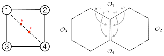
Figure 19: The contribution of two particles in the same $l=0$ mirror edge. There are two hexagons involved, and we call them left and right hexagons. By an explicit calculation, one verifies that it only contributes at four loops and beyond.

It will be shown in particular that it contributes only at four loops. Recall that the $a$-th mirror bound state $\mathcal{X}_{a}$ is composed from the tensor product of two factors belonging to the $a$-th antisymmetric representation of $\mathfrak{su}(2|2)$. A basis for this representation is $(\alpha_{i}=3,4)$

$$|\psi_{\alpha_{1}}\ldots\psi_{\alpha_{a}}\rangle+\ldots\,,\quad\quad\;\,\,\quad\;\,\,|\phi_{1}\psi_{\alpha_{1}}\ldots\psi_{\alpha_{a-1}}\rangle+\ldots\,,$$ (D.3)

$$|\phi_{2}\psi_{\alpha_{1}}\ldots\psi_{\alpha_{a-1}}\rangle+\dots\,,\quad\quad\;\,|\phi_{1}\phi_{2}\psi_{\alpha_{1}}\ldots\psi_{\alpha_{a-2}}\rangle+\ldots\,,\quad$$

where $(\phi_{1},\phi_{2},\psi_{3},\psi_{4})$ form an $\mathfrak{su}(2|2)$ fundamental multiplet, $a$ is called the bound state index, and the dots stand for permutations. As discussed in [11, 14], the basis above has to be modified for the hexagonalization procedure to reproduce the perturbative data. It is necessary to add so-called $Z$-markers to some of the basis states, and the prescription used here follows from the one given in the appendix A of [14]. The addition of $Z$-markers has two consequences: They give a contribution to the weight factors, and when one moves and removes them using the rules given in [15], one can get factors of momenta. Note that a rigorous explanation for the $Z$-marker prescription is still lacking. The dressing of the basis states is as follows (the bar denotes antiparticles)

$$\underbrace{|Z^{-t^{I}_{u}}\bar{\mathcal{X}}^{I}_{a}(u^{-\gamma})Z^{-t_{v}^{J}}\bar{\mathcal{X}}^{J}_{b}(v^{-\gamma})\rangle}_{\text{left hexagon}}\otimes\underbrace{|\mathcal{X}^{J}_{b}(v^{\gamma})Z^{t^{J}_{v}}\mathcal{X}^{I}_{a}(u^{\gamma})Z^{t_{u}^{I}}\rangle}_{\text{right hexagon}}\,,$$ (D.4)

where $\mathcal{X}_{a}^{I}(u)$ is a mirror magnon with bound state index $a$ and rapidity $u$, with $I$ being a (flavor) index for the $a$-th bound state representation, and $\gamma$ denotes the mirror transform that transports excitations from one edge of the hexagon to the next. The values of $t^{I}_{u}$ and $t^{J}_{v}$ depend on the field content of the bound-state basis elements, and whether one is considering the “$+$” or “$-$” dressing. The rules to find the values of the $t_{i}$ are:

“$$+ \text{dressing}: \psi_{\alpha} \rightarrow\psi_{\alpha}\,, \phi_{1} \rightarrow Z^{\frac{1}{2}}\phi_{1}\,, \phi_{2} \rightarrow Z^{-\frac{1}{2}}\phi_{2}\,,$$”

$$\psi_{\dot{\alpha}} \rightarrow\psi_{\dot{\alpha}}\,, \phi_{\dot{1}} \rightarrow Z^{-\frac{1}{2}}\phi_{\dot{1}}\,, \phi_{\dot{2}} \rightarrow Z^{\frac{1}{2}}\phi_{\dot{2}}\,,$$

“$$- \text{dressing}: \psi_{\alpha} \rightarrow\psi_{\alpha}\,, \phi_{1} \rightarrow Z^{-\frac{1}{2}}\phi_{1}\,, \phi_{2} \rightarrow Z^{\frac{1}{2}}\phi_{2}\,,$$”

$$\psi_{\dot{\alpha}} \rightarrow\psi_{\dot{\alpha}}\,, \phi_{\dot{1}} \rightarrow Z^{\frac{1}{2}}\phi_{\dot{1}}\,, \phi_{\dot{2}} \rightarrow Z^{-\frac{1}{2}}\phi_{\dot{2}}\,,$$ (D.5)

where undotted/dotted labels are left/right $\mathfrak{su}(2|2)$ fundamental indices, and the prescription is to average over the two different dressings at the end of the calculation. Within a hexagon form factor $\mathfrak{h}$, one can move all $Z$-markers to the left, and then remove them via the rules (see Appendices C and F in [15])

$$\chi Z\simeq e^{ip}Z\chi\,,\qquad\langle\mathfrak{h}|Z^{n}\Psi\rangle=z^{n}\langle\mathfrak{h}|\Psi\rangle\,,\qquad z^{2}=e^{-ip}\,,$$ (D.6)

where $\chi$ is a fundamental magnon, and $\Psi$ is a generic spin-chain state. When removing all $Z$-markers in this way, it is possible to show that for any value of $t^{I}_{u}$ and $t^{J}_{v}$, all momentum factors $e^{ip}$ cancel each other.

The hexagon form factors are matrices in flavor space. In what follows, we are going to work in the string frame, where the non-vanishing components of the one-particle hexagon form factors are

$$\mathfrak{h}^{1\dot{2}}=-\mathfrak{h}^{2\dot{1}}=1\,,\quad\quad\mathfrak{h}^{3\dot{4}}=-\mathfrak{h}^{4\dot{3}}=-i\,.$$ (D.7)

The contribution from two particles in the same zero-length bridge is the result of the following integral

$$\mathcal{M}^{(2)}_{\rm{same\,edge}}(z,\alpha)=\int\frac{du}{2\pi}\frac{dv}{2\pi}\sum_{a=1}^{\infty}\sum_{b=1}^{\infty}\sum_{I,J}\mu_{a}(u^{\gamma})\,\mu_{b}(v^{\gamma})\times\\ \times\mathfrak{h}\left[\bar{\mathcal{X}}^{I}_{a}(u^{-\gamma})\bar{\mathcal{X}}^{J}_{b}(v^{-\gamma})\right]\mathcal{W}\left[\mathcal{X}^{J}_{b}(v^{\gamma})\right]\mathcal{W}\left[\mathcal{X}^{I}_{a}(u^{\gamma})\right]\mathfrak{h}\left[\mathcal{X}^{J}_{b}(v^{\gamma})\mathcal{X}^{I}_{a}(u^{\gamma})\right]\,,$$ (D.10)

where the $\mu$’s are the measure factors, and the $\mathcal{W}$’s are weight factors associated to the particles whose origin is a $\mathrm{PSU}(2,2|4)$ transformation that aligns the frames of the two hexagons [11]. In order to simplify the calculation of the matrix part (flavor sums), it is convenient to use the following identity to have both hexagon form factors with the same crossed arguments:

$$\mathfrak{h}\left[\bar{\mathcal{X}}^{I}_{a}(u^{-\gamma})\bar{\mathcal{X}}^{J}_{b}(v^{-\gamma})\right]=(-1)^{\bar{I}}(-1)^{\bar{J}}\mathfrak{h}\left[\bar{\mathcal{X}}^{I\mathrm{c}}_{a}(u^{\gamma})\bar{\mathcal{X}}^{J\mathrm{c}}_{b}(v^{\gamma})\right]\,,$$ (D.11)

where the superscript $\mathrm{c}$ indicates that the indices $A$ and $\dot{A}$ of the excitations are swapped. The precise values for the signs can be deduced from the crossing rules [15, 64]

$$\chi^{a\dot{b}}\xrightarrow{\;2\gamma\;}\chi^{b\dot{a}}\,,\quad\chi^{\alpha\dot{\beta}}\xrightarrow{\;2\gamma\;}-\chi^{\beta\dot{\alpha}}\,,\quad\chi^{\alpha\dot{a}}\xrightarrow{\;2\gamma\;}\chi^{a\dot{\alpha}}\,,\quad\chi^{a\dot{\alpha}}\xrightarrow{\;2\gamma\;}-\chi^{\alpha\dot{a}}$$ (D.12)

for fundamental magnons $\chi$. In particular, one has

$$(-1)^{\bar{I}}=(-1)^{\sharp\,{\rm{scalars}}_{\bar{I}}\,+\,\dot{f}_{\bar{I}}}\,,$$ (D.13)

with $\dot{f}_{\bar{I}}$ the number of fermionic dotted indices. The weight factor $\mathcal{W}$ was computed in [11], and it was rewritten in [14] taking both the $Z$-markers prescription and the “$+$” and “$-$” dressings into account as

$$\mathcal{W}^{\pm}[\mathcal{X}_{a}^{I}(u^{\gamma})]=e^{-2i\tilde{p}_{a}(u^{\gamma}){\rm{log}}|z|}\,e^{iL^{I}\phi}\,e^{iR^{I}(\theta\pm\varphi)}\,,$$ (D.14)

where the angles were defined in (D.2), and the eigenvalues $L^{I}$ and $R^{I}$ of the generators $L$ and $R$ can be deduced from the action of these generators on the fundamental excitations given by (the dotted indices have opposite eigenvalues)

$$e^{iL}\psi^{1}=e^{\frac{i}{2}}\psi^{1}\,,\quad e^{iL}\psi^{2}=e^{-\frac{i}{2}}\psi^{2}\,,\quad e^{iR}\phi^{1}=e^{\frac{i}{2}}\phi^{1}\,,\quad e^{iR}\phi^{2}=e^{-\frac{i}{2}}\phi^{2}\,.$$ (D.15)

As a consequence of the formulas above, one has

$$\mathcal{M}^{(2)}_{\text{same edge}}(z,\alpha)=\int\frac{du}{2\pi}\frac{dv}{2\pi}\sum_{a=1}^{\infty}\sum_{b=1}^{\infty}\mu_{a}(u^{\gamma})\,\mu_{b}(v^{\gamma})\,h_{ab}(u^{\gamma},v^{\gamma})\,h_{ba}(v^{\gamma},u^{\gamma})\times\\ \times\,e^{-2i\tilde{p}_{a}(u^{\gamma})\log|z|}\,e^{-2i\tilde{p}_{b}(v^{\gamma})\log|z|}\,\mathcal{F}_{ab}\,.$$ (D.18)

Here, $\mathcal{F}_{ab}$ contains the matrix part and the flavor-dependent part of the weight factor. It is given by

$$\mathcal{F}_{ab}=\sum_{I,J}\,(-1)^{\bar{I}}(-1)^{\bar{J}}\,\mathcal{W}^{\pm}_{\text{flavor}}\left[\mathcal{X}^{J}_{b}(v^{\gamma})\right]\mathcal{W}^{\pm}_{{\rm{flavor}}}\left[\mathcal{X}^{I}_{a}(u^{\gamma})\right]\times\\ \times\langle\chi_{b}^{\bar{J}_{a}}(v^{\gamma})\chi_{a}^{\bar{I}_{a}}(u^{\gamma})|S|\chi_{a}^{\bar{I}_{b}}(u^{\gamma})\chi_{b}^{\bar{J}_{b}}(v^{\gamma})\rangle\,\langle\chi_{a}^{I_{b}}(u^{\gamma})\chi_{b}^{J_{b}}(v^{\gamma})|S|\chi_{b}^{J_{a}}(v^{\gamma})\chi_{a}^{I_{a}}(u^{\gamma})\rangle\,,$$ (D.21)

with $S$ being the mirror bound state $S$-matrix [14]. In principle, one can use the unitarity of the $S$-matrix to simplify the expression above, however one has to check that the weight factors do not spoil this simplification. Indeed, the $S$-matrix has a block-diagonal decomposition [65, 66, 14], and fixing the indices $J_{a}$ and $I_{a}$, one can show that the resulting states, after the action of the $S$-matrix, have a non-vanishing inner product only with definite weight-factor eigenstates, so indeed unitarity can be used. As an example, let us select a particular value of $J_{a}$ and $I_{a}$ to have the case Ia of [14], i. e. we have for some $k$ and $l$ that

$$|\chi_{b}^{J_{a}}(v^{\gamma})\chi_{a}^{I_{a}}(u^{\gamma})\rangle^{\rm{Ia}}=|k,l\rangle^{\rm{Ia}}\,,\quad{\rm{with}}\quad|k,l\rangle^{\rm{Ia}}=|\phi_{1}\psi_{1}^{b-k-1}\psi_{2}^{k}\rangle\otimes|\phi_{1}\psi_{1}^{a-l-1}\psi_{2}^{l}\rangle\,.$$ (D.22)

The $S$-matrix, when acting on a state of type Ia, produces a linear combination of states of type Ia of the form ($N=k+l$)

$$S\cdot|k,l\rangle^{{\rm{Ia}}}=\sum_{n=0}^{N}H^{k,l}_{n}\,|N-n,n\rangle^{{\rm{Ia}}}\,.$$ (D.23)

As a consequence of the equation above, all final states have precisely two $\phi_{1}$’s and the same total number of $\psi_{1}$’s and $\psi_{2}$’s. Thus they have non-zero inner products only with definitive weight-factor eigenstates, and this selects only a particular non-trivial set of values for $J_{b}$ and $I_{b}$. Using the unitarity of the $S$-matrix, we have

$$\mathcal{F}_{ab}=\frac{1}{2}\,(-1)^{a}(-1)^{b}\,(T^{+}_{a}T^{+}_{b}+T^{-}_{a}T^{-}_{b})\,,$$ (D.24)

where the factor of $1/2$ is present because we are averaging between the “$+$” and “$-$” dressings, and the $T^{\pm}$ are twisted transfer matrices given by

$$T^{\pm}_{a}=2(-1)^{a}\bigl{(}{\rm{cos}}\,\phi-{\rm{cos}}(\theta\pm\varphi)\bigr{)}\frac{{\rm{sin}}\,a\phi}{{\rm{sin}}\phi}\,.$$ (D.25)

Notice that the twisted transfer matrices are defined by

$$T^{\pm}_{a}={\rm{Tr}}_{a}\left[(-1)^{F}e^{iL\phi}e^{iR(\theta\pm\varphi)}\right]=\\ (-1)^{a}\left(e^{ia\phi}\sum_{n=0}^{a}e^{-2in\phi}-2\,{\rm{cos}}(\theta\pm\varphi)e^{i(a-1)\phi}\sum_{n=0}^{a-1}e^{-2in\phi}+e^{i(a-2)\phi}\sum_{n=0}^{a-2}e^{-2in\phi}\right)\,.$$ (D.28)

Substituting the expression for $\mathcal{F}_{ab}$ in (D.18), it only remains to evaluate the integral. Using the weak-coupling expansions given in Appendix C, it is easy to see that this contribution contributes only at four loops. The integral is easily evaluated by residues and at order $g^{8}$ it gives

$$\mathcal{M}^{(2)}_{\rm{same\,edge}}(z,\alpha)\Big{|}_{g^{8}}=-2\left[\frac{(z-\alpha)^{2}(\bar{z}-\alpha)^{2}}{\alpha^{2}}+\frac{(z-\bar{\alpha})^{2}(\bar{z}-\bar{\alpha})^{2}}{\bar{\alpha}^{2}}\right]\times\\ \times\left(\frac{1}{6}\left(F^{(2)}(z,\bar{z})\right)^{2}-\frac{1}{2}F^{(1)}(z,\bar{z})\,F^{(3)}(z,\bar{z})\right)\,,$$ (D.31)

where $F^{(1)}$, $F^{(2)}$ and $F^{(3)}$ were given in (4.4), (4.5), and (6.48). Another representation for $F^{(L)}$ is

$$F^{(L)}(z,\bar{z})=\frac{1}{z-\bar{z}}\left[\sum_{m=0}^{L}\frac{(-1)^{m}(2L-m)!}{L!(L-m)!m!}\,{\rm{log}}^{m}(z\bar{z})({\rm{Li}}_{2L-m}(z)-{\rm{Li}}_{2L-m}(\bar{z}))\right]\,.$$ (D.32)

D.3 The Three-Particle Contribution

Next, we compute the three-particle contribution, shown in both Figure 14 and Figure 20, using integrability. Note that this is a particular kind of three-particle contribution, as one can flip the line connecting the operators at positions $x_{1}$ and $x_{5}$, such that it connects the operators at position $x_{6}$ and $x_{4}$ instead. These two kinds of three-particle contributions are related by flipping invariance, and it is possible to deduce one from the other.

To compute the three-particle contribution, it is necessary to evaluate four hexagon form factors $\mathfrak{h}$, to use three weight factors $\mathcal{W}$ for gluing the hexagons together, and to sum over three mirror bound-state basis elements $\mathcal{X}^{I}$, whose bound state indices are going to be denoted by $a$, $b$, and $c$.

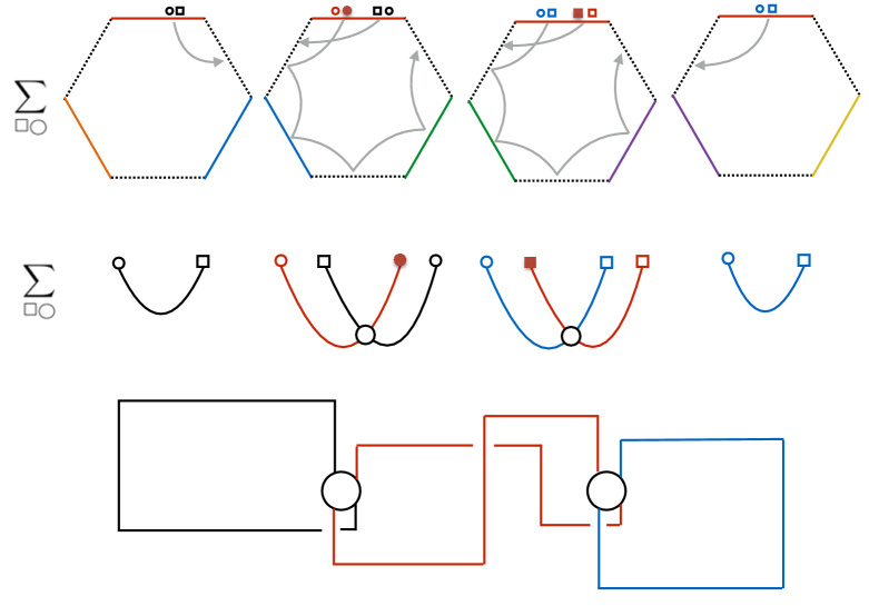
Figure 20: The figure at the top represents the four hexagons involved in the three-particle computation. The circles and the corresponding squares represent complementary sets of fundamental indices, i. e. if one of them equals $1$, then the other equals $2$, if one equals $3$, the other equals $4$, and vice versa, see [15]. The hexagons are glued together using three weight factors $\mathcal{W}$ (not shown in the figure). We have chosen to rotate some of the particles of the second and third hexagons by sequences of mirror transformations. The figure in the middle represents the contractions of the flavor indices, and the white circle with four lines denotes a mirror bound state $S$-matrix. The last figure schematically shows the sum over the indices denoted by circles and squares. The sum is not a straight trace, but rather is weighted by the three weight factors $\mathcal{W}$. We restrict ourselves to operators that lie in a common plane; in this case the weight factors are diagonal in the mirror state space. The result of the last figure is proportional to the three-particle matrix part. Note that it involves two mirror bound state $S$-matrices, and, unlike in the two-particle contribution, the sum represented by the red lines includes elements that are non-diagonal in the $\mathfrak{su}(2|2)$ preserved by the hexagon.

The three-particle contribution is given by the integral

$$\mathcal{M}^{(3)}(z_{1},z_{2},z_{3},\alpha_{1},\alpha_{2},\alpha_{3})=\\ \sum_{a=1}^{\infty}\sum_{b=1}^{\infty}\sum_{c=1}^{\infty}\int\frac{du_{1}}{2\pi}\frac{du_{2}}{2\pi}\frac{du_{3}}{2\pi}\,\mu_{a}(u_{1}^{\gamma})\,\mu_{b}(u_{2}^{\gamma})\,\mu_{c}(u_{3}^{\gamma})\sum_{I,J,K}\mathfrak{h}[\bar{\mathcal{X}}_{c}^{I}(u_{3}^{-\gamma})]\,\mathcal{W}[\mathcal{X}_{c}^{I}(u_{3}^{\gamma})]\times\mspace{60.0mu}\\ \times\mathfrak{h}[\mathcal{X}_{c}^{I}(u_{3}^{\gamma})\bar{\mathcal{X}}_{b}^{J}(u_{2}^{-\gamma})]\,\mathcal{W}[\mathcal{X}^{J}_{b}(u_{2}^{\gamma})]\,\mathfrak{h}[\mathcal{X}_{b}^{J}(u_{2}^{\gamma})\bar{\mathcal{X}}_{a}^{K}(u_{1}^{-\gamma})]\,\mathcal{W}[\mathcal{X}_{a}^{K}(u_{1}^{\gamma})]\,\mathfrak{h}[\mathcal{X}_{a}^{K}(u_{1}^{\gamma})]\,.$$ (D.36)

A naive basis, i. e. without the $Z$-markers, for the $a$-th mirror bound state $\mathcal{X}$ is given in (D.3). The dressing of the states by $Z$-markers with exponents $t_{i}$ appearing below are found using the rules of (D.5) . Notice the values of $t^{I}_{1}$, $t^{J}_{2}$ and $t^{K}_{3}$ depend on the field content of the bound state basis elements, and on whether one is considering the “$+$” or the “$-$” dressing. We have

$$\underbrace{|Z^{-t^{I}_{3}}\bar{\mathcal{X}}_{c}^{I}(u_{3}^{-\gamma})\rangle}_{\rm{left\,hexagon}}\otimes\underbrace{|\mathcal{X}^{I}_{c}(u_{3}^{\gamma})Z^{t^{I}_{3}}Z^{-t_{2}^{J}}\bar{\mathcal{X}}^{J}_{b}(u_{2}^{-\gamma})\rangle}_{\rm{second\,hexagon}}\otimes\underbrace{|\mathcal{X}^{J}_{b}(u_{2}^{\gamma})Z^{t^{J}_{2}}Z^{-t_{1}^{K}}\bar{\mathcal{X}}_{a}^{K}(u_{1}^{-\gamma})\rangle}_{\rm{third\,hexagon}}\otimes\underbrace{|\mathcal{X}_{a}^{K}(u_{1}^{\gamma})Z^{t_{1}^{K}}\rangle}_{\rm{right\,hexagon}}\,.$$ (D.37)

Moving all $Z$-markers to the left and removing them, one gets some non-trivial factors of momenta that will contribute to the integrand. The expression above is equal to

$$e^{it^{I}_{3}p(u_{2}^{\gamma})/2}e^{-it^{J}_{2}p(u_{3}^{\gamma})/2}e^{it^{J}_{2}p(u_{1}^{\gamma})/2}e^{-it^{K}_{1}p(u_{2}^{\gamma})/2}\,\times\\ \times\underbrace{|\bar{\mathcal{X}}^{I}_{c}(u_{3}^{-\gamma})\rangle}_{\rm{left\,hexagon}}\otimes\underbrace{|\mathcal{X}^{I}_{c}(u_{3}^{\gamma})\bar{\mathcal{X}}^{J}_{b}(u_{2}^{-\gamma})\rangle}_{\rm{second\,hexagon}}\otimes\underbrace{|\mathcal{X}^{J}_{b}(u_{2}^{\gamma})\bar{\mathcal{X}}^{K}_{a}(u_{1}^{-\gamma})\rangle}_{\rm{third\,hexagon}}\otimes\underbrace{|\mathcal{X}^{K}_{a}(u_{1}^{\gamma})\rangle}_{\rm{right\,hexagon}}\,.$$ (D.40)

A mirror particle-antiparticle pair is always created on a mirror edge shared by two hexagons. The particle is absorbed by one of the hexagons, the antiparticle is absorbed by the other hexagon. The weight factor originates in the symmetry transformation needed to bring both hexagons to the same frame—this transformation acts non-trivially on the mirror particles as one moves them from one hexagon to the other. The expression for the weight factor was given in (D.14), here we give its expression for the case with more cross ratios

$$\mathcal{W}^{\pm}[\mathcal{X}^{I}_{a_{i}}(u_{i}^{\gamma})]=e^{-2i\tilde{p}_{a_{i}}(u_{i}){\rm{log}}|z_{i}|}e^{iL^{I}\phi_{i}}e^{iR^{I}(\theta_{i}\pm\varphi_{i})}\,,$$ (D.41)

with

$$e^{i\phi_{i}}=\sqrt{\frac{z_{i}}{\bar{z}_{i}}}\,,\quad\quad e^{i\theta_{i}}=\sqrt{\frac{\alpha_{i}}{\bar{\alpha}_{i}}}\,,\quad\quad e^{i\varphi_{i}}=\sqrt{\frac{\alpha_{i}\bar{\alpha}_{i}}{z_{i}\bar{z}_{i}}}\,,$$ (D.42)

and the charges of the fundamental excitations under the generators $L$ and $R$ are given in (D.15).

In the expression (D.36), the hexagon form factors corresponding to the left and right hexagons only have one excitation. These hexagons have a trivial dynamical part and they contribute only with a possible sign that can be computed using a combination of the one-particle hexagon form factors given in (D.7). In addition, they imply that the excitations with rapidities $u_{1}$ and $u_{3}$ are both composed of transverse excitations only, and that their states are not changed by the scattering with the particles with rapidity $u_{2}$. As a matter of choice, we are going to mirror-rotate the two middle hexagon form factors before evaluating them. One has for the non-zero cases

$$\mathfrak{h}[\mathcal{X}_{c}^{I}(u_{3}^{\gamma})\bar{\mathcal{X}}_{b}^{J}(u_{2}^{-\gamma})]=(-1)^{\sharp\,{\rm{scalars}}_{\bar{J}}\,+\,f_{\bar{J}}}\,\mathfrak{h}[\bar{\mathcal{X}}_{b}^{Jc}(u_{2}^{5\gamma})\mathcal{X}_{c}^{I}(u_{3}^{\gamma})]\,,$$ (D.43)

with $f_{\bar{J}}$ the number of undotted fermionic indices in the set $\bar{J}$, and

$$\mathfrak{h}[\mathcal{X}_{b}^{J}(u_{2}^{\gamma})\bar{\mathcal{X}}_{a}^{K}(u_{1}^{-\gamma})]=(-1)^{a}\,\mathfrak{h}[\bar{\mathcal{X}}_{a}^{Kc}(u_{1}^{5\gamma})\mathcal{X}_{b}^{J}(u_{2}^{\gamma})]\,.$$ (D.44)

Notice that an important property of the dynamical factor of the hexagons that will be used below is

$$h_{ab}(u^{5\gamma},v^{\gamma})=\frac{1}{h_{ba}(v^{\gamma},u^{\gamma})}\,.$$ (D.45)

Collecting the expressions above, we have

$$\mathcal{M}^{(3)}(z_{1},z_{2},z_{3},\alpha_{1},\alpha_{2},\alpha_{3})=\sum_{a=1}^{\infty}\sum_{b=1}^{\infty}\sum_{c=1}^{\infty}\int\frac{du_{1}}{2\pi}\frac{du_{2}}{2\pi}\frac{du_{3}}{2\pi}\frac{\mu_{a}(u_{1}^{\gamma})\,\mu_{b}(u_{2}^{\gamma})\,\mu_{c}(u_{3}^{\gamma})}{h_{cb}(u_{3}^{\gamma},u_{2}^{\gamma})\,h_{ba}(u_{2}^{\gamma},u_{1}^{\gamma})}\times\\ \times e^{-2i\tilde{p}_{a}(u_{1}^{\gamma}){\log|z_{1}|}}\,e^{-2i\tilde{p}_{b}(u_{2}^{\gamma}){\log|z_{2}|}}\,e^{-2i\tilde{p}_{c}(u_{3}^{\gamma}){\log|z_{3}|}}\,\frac{1}{2}\,\mathcal{F}_{abc}\,,$$ (D.48)

with

$$\mathcal{F}_{abc}=\sum_{I,J,K}(-1)^{\sharp\,{\rm{scalars}}_{\bar{J}}\,+\,f_{\bar{J}}}\,(-1)^{a}\,e^{it^{I}_{3}p(u_{2}^{\gamma})/2}\,e^{-it^{J}_{2}p(u_{3}^{\gamma})/2}\,e^{it^{J}_{2}p(u_{1}^{\gamma})/2}\,e^{-it^{K}_{1}p(u_{2}^{\gamma})/2}\,\times\\ \times\mathfrak{h}[\bar{\mathcal{X}}_{c}^{I}(u_{3}^{-\gamma})]\,\mathcal{W}^{\pm}[\mathcal{X}_{c}^{I}(u_{3}^{\gamma})]\,\mathcal{W}^{\pm}[\mathcal{X}^{J}_{b}(u_{2}^{\gamma})]\,\mathcal{W}^{\pm}[\mathcal{X}_{a}^{K}(u_{1}^{\gamma})]\,\mathfrak{h}[\mathcal{X}_{a}^{K}(u_{1}^{\gamma})]\times\\ \times\langle\chi_{c}^{\bar{I}_{a}}(u_{3}^{\gamma})\chi_{b}^{\bar{J}_{a}}(u_{2}^{\gamma})|S|\chi_{b}^{\bar{J}_{b}}(u_{2}^{\gamma})\chi_{c}^{I_{a}}(u_{3}^{\gamma})\rangle\,\langle\chi_{b}^{J_{b}}(u_{2}^{\gamma})\chi_{a}^{\bar{K}_{a}}(u_{1}^{\gamma})|S|\chi_{a}^{K_{a}}(u_{1}^{\gamma})\chi_{b}^{J_{a}}(u_{2}^{\gamma})\rangle\,.$$ (D.52)

The mirror bound-state $S$-matrix using the “hybrid” convention was derived in [14] by adapting the derivation of the physical bound-state $S$-matrix of [66]. The $S$-matrix has a block-diagonal form, and it can be organized into three cases, depending on the values $(2,1,0,-1,-2)$ of the following charge (the superscripts 1 and 2 denotes the first and the second bound state being scattered)

$$C_{1}=\sharp\phi_{1}^{1}+\sharp\phi_{1}^{2}-\sharp\phi_{2}^{1}-\sharp\phi_{2}^{2}\,.$$ (D.53)

A basis for each case can be found in [14], and they are functions of two parameters $k$ and $l$ that are related with the number of fields $\psi_{2}$ within the bound states. The $S$-matrices are denoted by $H$, $Y$, and $Z$ for the cases I, II, and III respectively. Notice that the sum in $\mathcal{F}_{abc}$ has many terms, and each term involves a product of two $S$-matrix elements that, because of the sum in $J$ corresponding to the $u_{2}$ rapidity, can be diagonal or non-diagonal, see Figure 20. Some of the terms do not contribute at one-loop order, and to select the ones that do contribute, one has to analyze the dependence of the $S$-matrix elements on $g^{2}$. Using the results of [14], we have in a particular basis

$$H^{k,l}_{n}(u^{\gamma},v^{\gamma})\;\sim\;\mathcal{O}(1)\,,\quad\quad Y^{k,l}_{n}(u^{\gamma},v^{\gamma})\;\sim\;\left(\begin{array}[]{cccc}\mathcal{O}(1)&\mathcal{O}(g)&\mathcal{O}(g)&0\\ \mathcal{O}(g)&\mathcal{O}(1)&0&\mathcal{O}(g)\\ \mathcal{O}(\frac{1}{g})&0&\mathcal{O}(1)&\mathcal{O}(g)\\ 0&\mathcal{O}(\frac{1}{g})&\mathcal{O}(g)&\mathcal{O}(1)\end{array}\right)\,,$$ (D.58)

and

$$Z^{k,l}_{n}(u^{\gamma},v^{\gamma})\;\sim\;\left(\begin{array}[]{cccccc}\mathcal{O}(1)&\mathcal{O}(g)&\mathcal{O}(g)&\mathcal{O}(g^{2})&\mathcal{O}(g^{2})&\mathcal{O}(g^{2})\\ \mathcal{O}(\frac{1}{g})&\mathcal{O}(1)&\mathcal{O}(1)&\mathcal{O}(g)&\mathcal{O}(g)&\mathcal{O}(g)\\ \mathcal{O}(\frac{1}{g})&\mathcal{O}(1)&\mathcal{O}(1)&\mathcal{O}(g)&\mathcal{O}(g)&\mathcal{O}(g)\\ \mathcal{O}(1)&\mathcal{O}(\frac{1}{g})&\mathcal{O}(\frac{1}{g})&\mathcal{O}(1)&\mathcal{O}(1)&\mathcal{O}(1)\\ \mathcal{O}(1)&\mathcal{O}(g)&\mathcal{O}(g)&\mathcal{O}(g^{2})&\mathcal{O}(1)&\mathcal{O}(g^{2})\\ \mathcal{O}(1)&\mathcal{O}(g)&\mathcal{O}(g)&\mathcal{O}(g^{2})&\mathcal{O}(g^{2})&\mathcal{O}(1)\end{array}\right)\,.$$ (D.65)

As an example, let us evaluate one of the contributing terms of $\mathcal{F}_{abc}$, namely the term proportional to $\alpha_{1}\alpha_{2}\alpha_{3}$ (where $\alpha_{i}$ are the internal cross ratios, defined as in (3.3)). One can show that this term is obtained using the $+$ dressing and it only involves diagonal $S$-matrices elements. We have at one-loop order

$$\mathcal{F}_{abc}\big{|}^{g^{2}}_{\alpha_{1}\alpha_{2}\alpha_{3}}=-\sum_{m=0}^{a-1}\sum_{l=0}^{b-1}\sum_{k=0}^{c-1}(-1)^{a+c}(-1)^{b(a+c)}\sqrt{\frac{u_{3}^{2}+\frac{c^{2}}{4}}{u_{1}^{2}+\frac{a^{2}}{4}}}\times\\ \times\frac{1}{z_{1}z_{2}z_{3}}\left(\frac{z_{1}}{\bar{z}_{1}}\right)^{\frac{a}{2}-m}\left(\frac{z_{2}}{\bar{z}_{2}}\right)^{\frac{b}{2}-l}\left(\frac{z_{3}}{\bar{z}_{3}}\right)^{\frac{c}{2}-k}H^{m,l}_{m}(u_{1}^{\gamma},u_{2}^{\gamma})\,H^{l,k}_{l}(u_{2}^{\gamma},u_{3}^{\gamma})\,.$$ (D.68)

After computing $\mathcal{F}_{abc}$ at one loop, one has to perform the triple integration in (D.48). The integrand is singular for $a=b$ and/or $b=c$, because it has a pole lying on the integration line. We regularize the integral using the same $i\epsilon$ prescription used for the two-particle calculation of [14], described there in Appendix E. Basically, we close the contours of integration of $u_{3}$ and $u_{2}$ from below, and the contour of $u_{1}$ from above. With this choice of contours, we do not get the contributions from the poles $u_{1}=u_{2}$ and $u_{2}=u_{3}$, due to the $i\epsilon$ prescription. The integration can be done for chosen values of $a$, $b$, and $c$, and this generates a power series in $z_{1}$, $z_{2}$, and $z_{3}$. Taylor-expanding the result for the three-particle contribution given in (3.10), one can show that both series agree.

This concludes the integrability derivation of the three-particle result. As mentioned in the main text, the same result can be derived assuming that flip invariance holds. It would be very interesting to integrate (D.48) directly and get the full three-particle result instead of its Taylor expansion. We leave this for future work.

Appendix E The Planar $n$-Point Functions of BPS Operators and Non-1EI Graphs

In this Appendix, we further test the integrability formula for the $2n$-gon given in (3.15). We start by comparing the integrability result for the planar $n$-point functions of length-two BPS operators in a plane derived using this formula with the perturbative data at one loop computed in [67]. It will be shown that both results agree. In principle, one can compare the results for BPS operators of any length, however the combinatorics for the general case are complicated due to non-trivial cancellations among the different contributions. The argument for the general case will be based on the relation between the integrability results and the $\mathcal{N}=2$ formulation of $\mathcal{N}=4$ SYM that was also used in [13]. We end the Appendix with a discussion about non-one-edge-irreducible graphs at one loop. These graphs were expected to cancel among themselves for some cases, and they were excluded from the calculations of four- and five-point functions in [11, 14]. In this paper, the multi-particle mirror contributions were determined, and it is now possible to compute the contributions from all graphs without making any assumption. It will be shown that this will imply a refinement of the prescription of the sum over graphs of [11].

E.1 The Correlation Functions of $n$ BPS Operators

E.1.1 The Case of $n$ $20^{\prime}$ Operators

The connected planar one-loop correlation function of $n$ BPS operators of lengths $k_{i}$ was computed perturbatively in [67]. The result is

$$\langle\mathcal{O}_{k_{1}}(x_{1})\mathcal{O}_{k_{2}}(x_{2})\ldots\mathcal{O}_{k_{n}}(x_{n})\rangle\Big{|}_{\rm{connected}}^{g^{2}}=\\ \sum_{i,j,l,p}k_{i}k_{j}k_{l}k_{p}\;D_{ijlp}\operatorname{Disk}\Bigl{[}\mathcal{O}_{k_{i}-1}\mathcal{O}_{k_{j}-1}\mathcal{O}_{k_{l}-1}\mathcal{O}_{k_{p}-1};\;\prod_{\mathclap{m\neq\{i,j,l,p\}}}^{n}\mathcal{O}_{k_{m}}\Bigr{]}\,,$$ (E.3)

where the summation over $i,j,l,p$ is to be understood as follows. For every set of four different indices $\{i,j,l,p\}$, one has only three different terms in the sum, precisely $ijlp$, $iljp$ and $ijpl$. In addition, $\operatorname{Disk}$ means the tree-level correlation function with all the Wick contraction lines contained inside a disk, and with the operators listed in the first argument being inserted in the boundary of the disk, respecting their cyclic order, and the operators in the second argument inserted inside the disk. In evaluating the function $\operatorname{Disk}$, one also does not consider disconnected graphs. Notice that the four operators at the boundary of the disk are already connected to each other by interaction lines lying outside of the disk, and this has to be taken into account when classifying the disconnected graphs. As an example, the graph where all the operators at the boundary of the disk are not contracted with the ones inside the disk is disconnected. Finally, using the definition of $m$ given in (3.11),

$$D_{ijlp}=2m(z_{ijpl})d_{ip}d_{jl}+2m(z_{ipjl})d_{ij}d_{lp}\,,$$ (E.4)

with the cross ratios $z_{ijlk}$ being defined as

$$z_{ijkl}\bar{z}_{ijkl}=\frac{x_{ij}^{2}x_{kl}^{2}}{x_{ik}^{2}x_{jl}^{2}}\,,\quad\quad(1-z_{ijkl})(1-\bar{z}_{ijkl})=\frac{x_{il}^{2}x_{jk}^{2}}{x_{ik}^{2}x_{jl}^{2}}\,.$$ (E.5)

Notice that the function $D$ is invariant under both a reflection and a cyclic rotation of its indices due to the properties of the function $m$ given in (3.13). This is consistent with the fact that there are only three terms in the summation (E.3) for every set of four indices.

Here, we are going to consider the restriction of the general formula (E.3) to $k_{i}=2$ for all $i=1,\ldots,n$. Moreover, in order to compare the perturbative result with the integrability result, it is enough to consider the contribution to the sum in (E.3) coming from a definite set of four indices, say $\{1,2,3,4\}$ for definiteness. For this set of indices, we have that the sum on the right-hand side gives

$$\text{RHS of~{}\eqref{eq:DrukkerGeneral}}\big{|}_{\{1,2,3,4\}}=2^{4}\,D_{1234}\operatorname{Disk}\Bigl{[}\mathcal{O}^{1}_{1}\mathcal{O}^{2}_{1}\mathcal{O}^{3}_{1}\mathcal{O}^{4}_{1};\;\prod^{n}_{\mathclap{m\neq\{1,2,3,4\}}}\mathcal{O}^{m}_{2}\Bigr{]}+\\ +2^{4}\,D_{1324}\operatorname{Disk}\Bigl{[}\mathcal{O}^{1}_{1}\mathcal{O}^{3}_{1}\mathcal{O}^{2}_{1}\mathcal{O}^{4}_{1};\;\prod^{n}_{\mathclap{m\neq\{1,2,3,4\}}}\mathcal{O}^{m}_{2}\Bigr{]}+2^{4}\,D_{1243}\operatorname{Disk}\Bigl{[}\mathcal{O}^{1}_{1}\mathcal{O}^{2}_{1}\mathcal{O}^{4}_{1}\mathcal{O}^{3}_{1};\;\prod^{n}_{\mathclap{m\neq\{1,2,3,4\}}}\mathcal{O}^{m}_{2}\Bigr{]}\,.$$ (E.8)

The Disk correlation functions appearing above can be computed in a closed form. By the definition of the Disk function, one has to consider only connected planar correlators, and there are two distinct cases that have to be considered. Firstly, two neighboring boundary operators can contract, and the remaining operators form a string starting and ending on the remaining boundary operators. Secondly, it is possible to have two separate strings starting and ending on two neighboring boundary operators. We have, for example

$$\operatorname{Disk}\Bigl{[}\mathcal{O}^{1}_{1}\mathcal{O}^{2}_{1}\mathcal{O}^{3}_{1}\mathcal{O}^{4}_{1};\;\prod^{n}_{\mathclap{m\neq\{1,2,3,4\}}}\mathcal{O}^{m}_{2}\Bigr{]}=\;2^{(n-4)}\mspace{-50.0mu}\sum_{\begin{subarray}{c}i,j,k,l\,\in\,\{1,2,3,4\}\\ (i,j)\text{ and }(k,l)\text{ neighbors}\end{subarray}}\;\sum_{\begin{subarray}{c}\text{permutations}\\ \sigma\text{ of }\{5,\dotsc,n\}\end{subarray}}\biggl{[}d_{ij}d_{k\sigma(5)}d_{\sigma(5)\sigma(6)}\dotsc d_{\sigma(n)l}\\ +\sum_{p=5}^{n-1}d_{i\sigma(5)}d_{\sigma(5)\sigma(6)}\ldots d_{\sigma(p)j}d_{k\sigma(p+1)}d_{\sigma(p+1)\sigma(p+2)}\ldots d_{\sigma(n)l}\biggr{]}\,.$$ (E.11)

As an example application of the formula above, let us consider the following five-operator case

$$\operatorname{Disk}\left[\mathcal{O}^{1}_{1}\mathcal{O}^{2}_{1}\mathcal{O}^{3}_{1}\mathcal{O}^{4}_{1};\mathcal{O}^{5}_{2}\right]=2\,(d_{12}d_{35}d_{54}+d_{34}d_{15}d_{52}+d_{14}d_{25}d_{53}+d_{23}d_{15}d_{54})\,.$$ (E.12)

Using the formula (E.11), one can compute (E.8). Recall that the $D$ function given in (E.4) is a sum of two terms and each of them contains a function $m$ with some argument. In order to compare with the integrability computation, we can focus on the terms with $m(z_{1423})$ and $m(z_{1324})$, as the argument for the remaining terms is similar. Firstly, notice that

$$m(z_{1423})+m(z_{1324})=0\,,$$ (E.13)

and that both of these functions appear multiplied by $d_{12}d_{34}$ in $D_{1234}$ and $D_{1243}$ respectively. This implies that the contributions to (E.11) proportional to $m(z_{1423})$ and $m(z_{1324})$, consisting of strings of operators starting at the operators $\mathcal{O}_{1}$ and $\mathcal{O}_{3}$ and ending at the operators $\mathcal{O}_{2}$ and $\mathcal{O}_{4}$ respectively, cancel among themselves. For $m(z_{1423})$, one has the final result

$$\eqref{eq:Drukker1234first}\big{|}_{m(z_{1423})}=2^{n+1}m(z_{1423})\,d_{12}d_{34}\times\\ \times\mspace{-20.0mu}\sum_{\begin{subarray}{c}\text{permutations}\\ \sigma\text{ of }\{5,\dotsc,n\}\end{subarray}}\biggl{[}d_{14}d_{2\sigma(5)}d_{\sigma(5)\sigma(6)}\dotsc d_{\sigma(n)3}+\,d_{23}d_{1\sigma(5)}d_{\sigma(5)\sigma(6)}\ldots d_{\sigma(n)4}\\[-8.61108pt] +\sum_{p=5}^{n-1}d_{1\sigma(5)}d_{\sigma(5)\sigma(6)}\ldots d_{\sigma(p)4}d_{2\sigma(p+1)}d_{\sigma(p+1)\sigma(p+2)}\ldots d_{\sigma(n)3}\biggr{]}\,.$$ (E.17)

The next step is to compare the above result with the integrability calculation. The integrability result can be obtained by using the formula for the 2$n$-gon given in (3.15). The argument of the function $m$ appearing in that formula is given by the cross ratios

$$z_{i,j}\bar{z}_{i,j}=\frac{x_{i,j+1}^{2}x^{2}_{i+1,j}}{x^{2}_{i,i+1},x^{2}_{j,j+1}}\,,\quad(1-z_{i,j})(1-\bar{z}_{i,j})=\frac{x_{i,j}^{2}x^{2}_{i+1,j+1}}{x^{2}_{i,i+1}x^{2}_{j,j+1}}\,.$$ (E.18)

where $i$ and $j$ labels the operators in the polygon with $i\neq j$, $i+1\neq j$ and $i\neq j+1$ modulo $n$. The cross ratios $z_{ijkl}$ were defined in (E.5) and they are related with $z_{i,j}$ by

$$z_{i,j}=z_{i,j+1,i+1,j}\,.$$ (E.19)

The connected tree-level graphs of $n$ length-two BPS operators consist of polygons with $n$ vertices. The integrability computation, assuming that disconnected tree-level graphs give zero contribution, consist in using the 2$n$-gon formula of (3.15) for the tree-level connected polygons. Note that the internal and the external polygons give the same result, hence one gets a factor of two. The terms proportional to $m(z_{1423})$ are generated by polygons where $(i,i+1)=(1,2)$ and $(j,j+1)=(3,4)$ for some $i$ and $j$, as consequence of the relation (E.19). Summing over all possible polygons, it is not difficult to see that the integrability result agrees with the perturbative result of (E.17). The argument is similar for the other terms $m(z_{ijkl})$, and this proves the equality of both computation methods.

E.1.2 The Case of $n$ Arbitrary BPS Operators

We have shown above that the integrability result for the $n$-point function of length-two BPS operators agrees with the perturbative answer. The perturbative result was computed using the general result for correlation function of BPS operators described by Drukker and Plefka [67]. In principle, one can use a similar procedure as above for proving the equality for general BPS operators. However, the combinatorics for the general case are more complicated, and one has to take into account nontrivial cancellations between terms with different $D(z_{ijkl})$. We are going to argue that the integrability result agrees with the perturbative result by using the $\mathcal{N}=2$ off-shell superfield formulation of $\mathcal{N}=4$ SYM as discussed in [68, 13].

The $\mathcal{N}=4$ supermultiplet decomposes into a $\mathcal{N}=2$ supermultiplet and a hypermultiplet. When computing a correlation function of BPS operators, it is possible to restrict the polarization vectors to a certain subspace, and treat the external operators as containing only hypermultiplets. The polarization vectors $Y$ (we called these $\alpha_{i}$ for most of this work) were parametrized as a function of a complex parameter $\beta_{i}$ in [13] as follows

$$Y_{\beta_{i}}=\left(\frac{1+\beta_{i}\bar{\beta}_{i}}{2},i\frac{1-\beta_{i}\bar{\beta}_{i}}{2},i\,{\rm{Im}}\,\beta_{i},i\,{\rm{Re}}\,\beta_{i},0,0\right)\,.$$ (E.20)

Notice that the polarizations above give, for a generic value of the parameters $\beta_{i}$, a non-zero inner product between two arbitrary polarizations vectors. This property of the polarizations is important for the integrability computation, since when some of the inner products are zero, it is necessary to consider deformed graphs, as for example in the subleading computation of Section 6.2.2. By a direct computation one has

$$Y_{\beta_{i}}\cdot Y_{\beta_{j}}=y_{ij}^{2}=(\beta_{i}-\beta_{j})(\bar{\beta}_{i}-\bar{\beta}_{j})\,.$$ (E.21)

The one-loop correlation functions in the $\mathcal{N}=2$ superfield formalism are computed by inserting $\mathcal{N}=2$ YM lines in all possible ways in all tree-level graphs, see [13] for details. Take two edges of a tree-level graph, one connecting the operators $\mathcal{O}_{i}$ and $\mathcal{O}_{j}$ and the other connecting the operators $\mathcal{O}_{k}$ and $\mathcal{O}_{l}$. Deleting two propagators and respecting the cyclic order, one inserts the following function for computing the one-loop correction:

$$F_{ij;kl}=\frac{g^{2}}{2}T_{ij;kl}\,d_{ij}d_{kl}\,g_{ijkl}\,\tilde{F}_{ij;kl}\,,$$ (E.22)

where $T_{ij;kl}$ is a color factor, $d_{ij}=y^{2}_{ij}/x_{ij}^{2}$, and

$$\tilde{F}_{ij;kl}=x_{il}^{2}x^{2}_{jk}-x_{ik}^{2}x_{jl}^{2}-x_{ij}^{2}x_{kl}^{2}\left(\frac{y^{2}_{il}y^{2}_{jk}}{y^{2}_{ij}y^{2}_{kl}}-\frac{y^{2}_{ik}y^{2}_{jl}}{y^{2}_{ij}y^{2}_{kl}}\right)\,,\quad g_{ijkl}=\frac{1}{\pi^{2}}\int\frac{d^{4}x_{a}}{x^{2}_{ai}x^{2}_{aj}x^{2}_{ak}x^{2}_{al}}\,.$$ (E.23)

Defining the following cross ratios (similar definitions apply to the $R$-charge cross ratios $\alpha_{ijkl}$)

$$\tilde{z}_{ijkl}\tilde{\bar{z}}_{ijkl}=\frac{x^{2}_{ik}x^{2}_{jl}}{x^{2}_{ij}x^{2}_{kl}}\,,\quad(1-\tilde{z}_{ijkl})(1-\tilde{\bar{z}}_{ijkl})=\frac{x^{2}_{il}x^{2}_{jk}}{x^{2}_{ij}x_{kl}^{2}}\,,$$ (E.24)

it is possible to rewrite (E.22) as

$$F_{ij;kl}=-T_{ij;kl}\,d_{ij}d_{kl}\,m(z_{ijkl})\,,$$ (E.25)

where the function $m(z)$ is defined in (3.11), and it is the same function appearing in the formula of the 2$n$-gon. It is possible to get rid of the minus sign above by using the last of the $m$ function identities given in (3.13), and by changing variables $z_{ijkl}=(1-z_{i,k})$.

In the integrability calculation, one hexagonalizes the tree-level graphs and corrects the tree-level result by adding the mirror-particle contributions. It follows from using (E.25) that disconnected tree-level graphs give perturbatively zero contribution at one-loop order, and the only tree-level graphs that one has to consider are connected graphs that decompose the sphere into a set of polygonal faces. It is hard to prove using integrability that disconnected graphs give a zero contribution at one loop, as the calculation involves loops and spirals. See Appendix F for details. However, using our prescription, it is possible to argue that they vanish, and all the integrability contributions from any planar graph can be calculated using the $2n$-gon formula. Due to the fact that the same function $m$ appears in the $2n$-gon integrability formula and in the perturbative building block $F_{ij;kl}$ defined above, it is easy to see that the integrability result agrees with the perturbative result for general $n$-point functions of BPS operators. In particular, this implies the non-renormalization of the extremal and next-to-extremal correlation functions by integrability, as mentioned in Section 3.2.

E.2 On Non-1EI Graphs

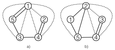
Figure 21: The two kinds of non-1EI graphs that appear in the computation of a five-point function of three length-two and two length-three BPS operators. The perturbative result was reproduced by an integrability calculation in [14] without considering these graphs, in other words their contributions must vanish. In this paper we have computed the $n$-particle contribution, and show that they indeed give a zero contribution.

The connected graphs were classified into two types in [11]: The one-edge irreducible (1EI) graphs and the non-1EI graphs. By definition, 1EI graphs are graphs that do not become disconnected when a set of lines connecting any two operators are cut. Typically, non-1EI graphs have more zero-length bridges, hence their calculations using integrability are harder because they involve more multi-particle contributions. In this work, we have computed these integrability contributions, and we are in a position to evaluate all non-1EI planar graphs without making any assumption about them.

We start by showing that the non-1EI graphs not considered in the analysis of the five-point function of three length-two and two length-three BPS operators done in [14] do indeed vanish. The graphs are shown in Figure 21. Considering that the five-point function lies in a plane, there are four spacetime cross ratios characterizing it (similarly for the $R$-charge cross ratios). They are given by

$$z\bar{z}=\frac{x_{12}^{2}x_{34}^{2}}{x_{13}^{2}x_{24}^{2}}\,,\quad(1-z)(1-\bar{z})=\frac{x_{14}^{2}x_{23}^{2}}{x_{13}^{2}x_{24}^{2}}\,,\quad w\bar{w}=\frac{x_{15}^{2}x_{34}^{2}}{x_{13}^{2}x_{54}^{2}}\,,\quad(1-w)(1-\bar{w})=\frac{x_{14}^{2}x_{35}^{2}}{x_{13}^{2}x_{45}^{2}}\,.$$ (E.26)

One can use the 2$n$-gon formula of (3.15) to compute the integrability result for these graphs. The relevant polygons have the edges

$${\rm{Diagram}}\,\,a)\,=\{1,5,3,4,2,4,3,5\}\,,\quad{\rm{Diagram}}\,\,b)\,=\{1,2,5,4,3,4,5\}\,.$$ (E.27)

Using the properties of the functions $m$ given in (3.13), it is possible to show that indeed the graphs of Figure 21 give a zero one-loop contribution, and the comparison between integrability and the perturbative data of [14] is correct.

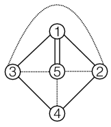
Figure 22: One non-1EI graph contributing to the five-point function of four length-two and one length-four BPS operators. Contrary to the original expectation, this graph gives a non-zero contribution from the integrability calculation. This requires a refinement of the prescription for summing over graphs of [11].

In [11], the prescription for summing over graphs was to not include non-1EI graphs in the summation, because they were expected to vanish. Using this prescription, the four-point functions of arbitrary BPS operators and some five-point functions were computed using integrability, and the result agreed with perturbation theory. Nevertheless, the general case for $n$-point functions is more complicated even at one loop. In Figure 22, we show an example of a non-vanishing one-loop non-1EI graph for the case of four length-two and one length-four BPS operator, as one can see by computing the graph using the $2n$-gon expression of (3.15) (it gives two times the one-particle contribution of the square). This result contradicts the assumptions of the prescription that has to the refined. The correct prescription is to sum over all graphs including both 1EI and non-1EI graphs. This gives the correct result for arbitrary one-loop planar correlation functions of BPS operators, as argued in the previous subsection using YM insertion lines.

Appendix F Contributions from Disconnected Graphs

In this appendix, we discuss disconnected planar graphs on the sphere, and argue that their contribution to the planar four-point function vanishes at one loop (in agreement with perturbation theory). In fact, there is only one disconnected planar four-point graph; it is depicted in Figure 23, including its hexagonalization. Much like the secretly planar graphs discussed in the main text, this graph corresponds to a degenerate Riemann surface, namely a sphere which splits into two connected components. We therefore need to consider Dehn-twist identifications as well as the subtraction of the degenerate case in order to correctly evaluate its contribution.

As shown in the figure, the graph has a cycle formed by the zero-length bridges, and one has to identify magnon configurations that are related by Dehn twists performed on this cycle. As in the case of secretly planar graphs discussed in the main text, we conjecture that the net effect of the Dehn twist is to identify configurations that include closed loops of magnon with the analogous configurations without any loops. For the tessellation we chose, the only configuration that does not contain a loop (and that “feels” all the four-operators) is the one depicted in Figure 23 (on the left). The contribution from this configuration is given by $\mathop{\texttt{polygon}}(1,3,1,2,4,2)$, which evaluates to zero owing to the pinching rule.

Having evaluated the contribution from the disconnected graph on the sphere, the next task is to evaluate the subtraction, which comes from two spheres, each with two operator insertions and a single marked point (on the right in Figure 23). As discussed in Section 2.4, their contributions are related to the one without marked points by a shift of the gauge group rank. Since the (planar) two-point functions do not receive loop corrections, this immediately shows that the contribution from the subtraction is zero for our case.

Therefore, in summary, we have $(0-0)=0$, which shows that the disconnected graphs do not contribute at one loop, as claimed in the beginning of this section.

Figure 23: In the left figure, we depict a disconnected graph drawn on a sphere, including its hexagonalization. The solid lines are non-zero-length bridges, while the dashed lines denote zero-length bridges. The red dots are a combination of magnons that can potentially contribute at one loop. On the right, we drew a corresponding subtraction graph which is given by two disconnected spheres, each with one marked point.

References

- [1] T. Bargheer, J. Caetano, T. Fleury, S. Komatsu and P. Vieira, “Handling Handles I: Nonplanar Integrability”, arxiv:1711.05326.
- [2] S. S. Razamat, “On a worldsheet dual of the Gaussian matrix model”, JHEP 0807, 026 (2008), arxiv:0803.2681.
- [3] R. Gopakumar, “From free fields to AdS”, Phys. Rev. D70, 025009 (2004), hep-th/0308184.
- [4] R. Gopakumar, “From free fields to AdS. 2.”, Phys. Rev. D70, 025010 (2004), hep-th/0402063.
- [5] R. Gopakumar, “Free field theory as a string theory?”, Comptes Rendus Physique 5, 1111 (2004), hep-th/0409233, in: “Annual International Conference on Strings, Theory and Applications (Strings 2004) Paris, France, 28 June - July 2, 2004”, pp. 1111-1119.
- [6] R. Gopakumar, “From free fields to AdS: III”, Phys. Rev. D72, 066008 (2005), hep-th/0504229.
- [7] O. Aharony, Z. Komargodski and S. S. Razamat, “On the worldsheet theories of strings dual to free large N gauge theories”, JHEP 0605, 016 (2006), hep-th/0602226.
- [8] O. Aharony, J. R. David, R. Gopakumar, Z. Komargodski and S. S. Razamat, “Comments on worldsheet theories dual to free large N gauge theories”, Phys. Rev. D75, 106006 (2007), hep-th/0703141.
- [9] K. Strebel, “Quadratic differentials”, Springer (1984).
- [10] M. Mulase and M. Penkava, “Ribbon Graphs, Quadratic Differentials on Riemann Surfaces, and Algebraic Curves Defined over ”, math-ph/9811024.
- [11] T. Fleury and S. Komatsu, “Hexagonalization of Correlation Functions”, JHEP 1701, 130 (2017), arxiv:1611.05577.
- [12] B. Eden and A. Sfondrini, “Tessellating cushions: four-point functions in 4 SYM”, JHEP 1710, 098 (2017), arxiv:1611.05436.
- [13] B. Eden, Y. Jiang, D. le Plat and A. Sfondrini, “Colour-dressed hexagon tessellations for correlation functions and non-planar corrections”, JHEP 1802, 170 (2018), arxiv:1710.10212.
- [14] T. Fleury and S. Komatsu, “Hexagonalization of Correlation Functions II: Two-Particle Contributions”, JHEP 1802, 177 (2018), arxiv:1711.05327.
- [15] B. Basso, S. Komatsu and P. Vieira, “Structure Constants and Integrable Bootstrap in Planar 4 SYM Theory”, arxiv:1505.06745.
- [16] J. Escobedo, N. Gromov, A. Sever and P. Vieira, “Tailoring Three-Point Functions and Integrability”, JHEP 1109, 028 (2011), arxiv:1012.2475.
- [17] J. Escobedo, N. Gromov, A. Sever and P. Vieira, “Tailoring Three-Point Functions and Integrability II. Weak/strong coupling match”, JHEP 1109, 029 (2011), arxiv:1104.5501.
- [18] N. Gromov, A. Sever and P. Vieira, “Tailoring Three-Point Functions and Integrability III. Classical Tunneling”, JHEP 1207, 044 (2012), arxiv:1111.2349.
- [19] N. Gromov and P. Vieira, “Quantum Integrability for Three-Point Functions of Maximally Supersymmetric Yang–Mills Theory”, Phys. Rev. Lett. 111, 211601 (2013), arxiv:1202.4103.
- [20] N. Gromov and P. Vieira, “Tailoring Three-Point Functions and Integrability IV. Theta-morphism”, JHEP 1404, 068 (2014), arxiv:1205.5288.
- [21] J. Caetano and T. Fleury, “Three-point functions and spin chains”, JHEP 1409, 173 (2014), arxiv:1404.4128.
- [22] Y. Kazama and S. Komatsu, “On holographic three point functions for GKP strings from integrability”, JHEP 1201, 110 (2012), arxiv:1110.3949.
- [23] Y. Kazama and S. Komatsu, “Wave functions and correlation functions for GKP strings from integrability”, JHEP 1209, 022 (2012), arxiv:1205.6060.
- [24] Y. Kazama and S. Komatsu, “Three-point functions in the SU(2) sector at strong coupling”, JHEP 1403, 052 (2014), arxiv:1312.3727.
- [25] D. Gaiotto, G. W. Moore and A. Neitzke, “Four-dimensional wall-crossing via three-dimensional field theory”, Commun. Math. Phys. 299, 163 (2010), arxiv:0807.4723.
- [26] D. Gaiotto, G. W. Moore and A. Neitzke, “Wall-crossing, Hitchin Systems, and the WKB Approximation”, arxiv:0907.3987.
- [27] B. Basso, V. Gonçalves, S. Komatsu and P. Vieira, “Gluing Hexagons at Three Loops”, Nucl. Phys. B907, 695 (2016), arxiv:1510.01683.
- [28] Y. Jiang, S. Komatsu, I. Kostov and D. Serban, “Clustering and the Three-Point Function”, J. Phys. A49, 454003 (2016), arxiv:1604.03575.
- [29] L. Chekov, “Matrix model for discretized moduli space”, J. Geom. Phys. 12, 153 (1993), hep-th/9205106.
- [30] L. Chekhov, “Matrix models and geometry of moduli spaces”, hep-th/9509001.
- [31] D. Anselmi, “Nodes as composite operators in matrix models”, Class. Quant. Grav. 12, 1135 (1995), hep-th/9411206.
- [32] G. ’t Hooft, “A Planar Diagram Theory for Strong Interactions”, Nucl. Phys. B72, 461 (1974).
- [33] T. Bargheer, F. Coronado and P. Vieira, “Large-Charge Correlators from Octagons”, to appear.
- [34] T. Bargheer, F. Coronado, V. Gonçalves and P. Vieira, work in progress.
- [35] N. Beisert, “The su(22) dynamic S-matrix”, Adv. Theor. Math. Phys. 12, 945 (2008), hep-th/0511082.
- [36] N. Beisert, R. Hernández and E. López, “A Crossing-symmetric phase for strings”, JHEP 0611, 070 (2006), hep-th/0609044.
- [37] B. Eden, Y. Jiang, M. de Leeuw, T. Meier, D. le Plat and A. Sfondrini, “Positivity of hexagon perturbation theory”, arxiv:1806.06051.
- [38] M. Mulase and M. Penkava, “Combinatorial Structure of the Moduli Space of Riemann Surfaces and the KP Equation”, unpublished, http://www.math.ucdavis.edu/~mulase/texfiles/1997moduli.pdf.
- [39] M. Ademollo, A. D’Adda, R. D’Auria, F. Gliozzi, E. Napolitano, S. Sciuto and P. Di Vecchia, “Soft Dilations and Scale Renormalization in Dual Theories”, Nucl. Phys. B94, 221 (1975).
- [40] E. D’Hoker, D. Z. Freedman, S. D. Mathur, A. Matusis and L. Rastelli, “Extremal correlators in the AdS/CFT correspondence”, hep-th/9908160, in: “The Many Faces of the Superworld”, Yuri Golfand Memorial Volume, ed.: M. Shifman, World Scientific (1999), Singapore.
- [41] B. Eden, P. S. Howe, C. Schubert, E. Sokatchev and P. C. West, “Extremal correlators in four-dimensional SCFT”, Phys. Lett. B472, 323 (2000), hep-th/9910150.
- [42] B. U. Eden, P. S. Howe, E. Sokatchev and P. C. West, “Extremal and next-to-extremal n point correlators in four-dimensional SCFT”, Phys. Lett. B494, 141 (2000), hep-th/0004102.
- [43] G. Arutyunov and E. Sokatchev, “On a large N degeneracy in 4 SYM and the AdS/CFT correspondence”, Nucl. Phys. B663, 163 (2003), hep-th/0301058.
- [44] G. Arutyunov, S. Penati, A. Santambrogio and E. Sokatchev, “Four point correlators of BPS operators in 4 SYM at order ”, Nucl. Phys. B670, 103 (2003), hep-th/0305060.
- [45] G. Arutyunov, F. A. Dolan, H. Osborn and E. Sokatchev, “Correlation functions and massive Kaluza-Klein modes in the AdS/CFT correspondence”, Nucl. Phys. B665, 273 (2003), hep-th/0212116.
- [46] J. Drummond, C. Duhr, B. Eden, P. Heslop, J. Pennington and V. A. Smirnov, “Leading singularities and off-shell conformal integrals”, JHEP 1308, 133 (2013), arxiv:1303.6909.
- [47] V. G. Knizhnik, “Analytic Fields on Riemann Surfaces. 2”, Commun. Math. Phys. 112, 567 (1987).
- [48] L. Motl, “Proposals on nonperturbative superstring interactions”, hep-th/9701025.
- [49] R. Dijkgraaf, E. P. Verlinde and H. L. Verlinde, “Matrix string theory”, Nucl. Phys. B500, 43 (1997), hep-th/9703030.
- [50] D. J. Gross and P. F. Mende, “The High-Energy Behavior of String Scattering Amplitudes”, Phys. Lett. B197, 129 (1987).
- [51] D. J. Gross and P. F. Mende, “String Theory Beyond the Planck Scale”, Nucl. Phys. B303, 407 (1988).
- [52] P. F. Mende and H. Ooguri, “Borel Summation of String Theory for Planck Scale Scattering”, Nucl. Phys. B339, 641 (1990).
- [53] S. H. Shenker, “The Strength of nonperturbative effects in string theory”, in: “Random Surfaces and Quantum Gravity”, Proceedings of the Cargèse Workshop, 27 May – 2 June 1990, pp. 191-200, ed.: O. Alvarez, E. Marinari and P. Windey, Plenum Press (1991), New York.
- [54] L. F. Alday and G. P. Korchemsky, “Revisiting instanton corrections to the Konishi multiplet”, JHEP 1612, 005 (2016), arxiv:1605.06346.
- [55] L. F. Alday and G. P. Korchemsky, “Instanton corrections to twist-two operators”, JHEP 1706, 008 (2017), arxiv:1609.08164.
- [56] L. F. Alday and G. P. Korchemsky, “On instanton effects in the operator product expansion”, JHEP 1705, 049 (2017), arxiv:1610.01425.
- [57] G. P. Korchemsky, “Instanton effects in correlation functions on the light-cone”, JHEP 1712, 093 (2017), arxiv:1704.00448.
- [58] G. Grignani, P. Orland, L. D. Paniak and G. W. Semenoff, “Matrix theory interpretation of DLCQ string world sheets”, Phys. Rev. Lett. 85, 3343 (2000), hep-th/0004194.
- [59] E. Bergshoeff, J. Gomis and Z. Yan, “Nonrelativistic String Theory and T-Duality”, arxiv:1806.06071.
- [60] R. Ben-Israel, A. G. Tumanov and A. Sever, “Scattering amplitudes – Wilson loops duality for the first non-planar correction”, JHEP 1808, 122 (2018), arxiv:1802.09395.
- [61] N. Gromov, V. Kazakov, S. Leurent and D. Volin, “Quantum Spectral Curve for Planar 4 Super-Yang–Mills Theory”, Phys. Rev. Lett. 112, 011602 (2014), arxiv:1305.1939.
- [62] A. Cavaglià, N. Gromov and F. Levkovich-Maslyuk, “Quantum Spectral Curve and Structure Constants in 4 SYM: Cusps in the Ladder Limit”, JHEP 1810, 060 (2018), arxiv:1802.04237.
- [63] S. Giombi and S. Komatsu, “Exact Correlators on the Wilson Loop in 4 SYM: Localization, Defect CFT, and Integrability”, JHEP 1805, 109 (2018), arxiv:1802.05201.
- [64] J. Caetano and T. Fleury, “Fermionic Correlators from Integrability”, JHEP 1609, 010 (2016), arxiv:1607.02542.
- [65] G. Arutyunov and S. Frolov, “The S-matrix of String Bound States”, Nucl. Phys. B804, 90 (2008), arxiv:0803.4323.
- [66] G. Arutyunov, M. de Leeuw and A. Torrielli, “The Bound State S-Matrix for Superstring”, Nucl. Phys. B819, 319 (2009), arxiv:0902.0183.
- [67] N. Drukker and J. Plefka, “The Structure of n-point functions of chiral primary operators in 4 super Yang–Mills at one-loop”, JHEP 0904, 001 (2009), arxiv:0812.3341.
- [68] P. S. Howe, C. Schubert, E. Sokatchev and P. C. West, “Explicit construction of nilpotent covariants in 4 SYM”, Nucl. Phys. B571, 71 (2000), hep-th/9910011.