On Reinforcement Learning for Full-length Game of StarCraft
Abstract
StarCraft II poses a grand challenge for reinforcement learning. The main difficulties include huge state space, varying action space, long horizon, etc. In this paper, we investigate a set of techniques of reinforcement learning for the full-length game of StarCraft II. We investigate a hierarchical approach, where the hierarchy involves two levels of abstraction. One is the macro-actions extracted from expert’s demonstration trajectories, which can reduce the action space in an order of magnitude yet remains effective. The other is a two-layer hierarchical architecture, which is modular and easy to scale. We also investigate a curriculum transfer learning approach that trains the agent from the simplest opponent to harder ones. On a 6464 map and using restrictive units, we train the agent on a single machine with 4 GPUs and 48 CPU threads. We achieve a winning rate of more than 99% against the difficulty level-1 built-in AI. Through the curriculum transfer learning algorithm and a mixture of combat model, we can achieve over 93% winning rate against the most difficult non-cheating built-in AI (level-7) within days. We hope this study could shed some light on the future research of large-scale reinforcement learning.
1 Introduction
In recent years, reinforcement learning (?) (RL) has developed rapidly in many different domains. The game of Go has been considered conquered after AlphaGo (?) and AlphaGo Zero (?) . Many Atari games are nearly solved using DQN (?) and follow-up methods. Various mechanical control problems, such as robotic arms (?) and self-driving vehicles (?), have made great progress. However, reinforcement learning algorithms at present are still difficult to be used in large-scale reinforcement learning problem. Agents can not learn to solve problems as smartly and efficiently as humans. In order to improve the ability of reinforcement learning, complex strategic games like StarCraft have become the perfect simulation environments for many institutions such as DeepMind (?), FAIR (?), and Alibaba (?).
From the perspective of reinforcement learning, StarCraft is a very difficult problem. Firstly, it is an imperfect information game. Players can only see a small area of map through a local camera and there is a fog of war in the game. Secondly, the state space and action space of StarCraft are huge. StarCraft’s image size is much larger than that of Go. There are hundreds of units and buildings, and each of them has unique operations, making action space extremely large. Thirdly, a full-length game of StarCraft usually lasts from 30 minutes to more than an hour, and players need to make thousands of decisions to win. Finally, StarCraft is a multi-agent game. The combination of these issues makes StarCraft a great challenge for reinforcement learning.
Most previous agents in StarCraft are based on manual rules and scripts. Some works related to reinforcement learning are usually about micromanagement (e.g. (?)) and macromanagement (e.g. (?)). These works solved some specific problems like local combat in StarCraft. However, there are rare works about the full-length games. In the paper of SC2LE (?), the benchmark result given by DeepMind shows that the A3C algorithm (?) in SC2LE did not achieve one victory on the easiest level-1, which reveals the difficulty of the full-length game in StarCraft II. In the next section, we will have a summary of the difficulties encountered in the StarCraft II and introduce the simulation platform SC2LE (StarCraft II Learning Environment).
In this paper, we investigate a set of techniques of reinforcement learning for the full-length game of StarCraft II (SC2). In the section following the background, we present the hierarchical architecture investigated in this paper, which uses several levels of abstractions to make intractable large-scale reinforcement learning problems easier to handle. An effective training algorithm tailed to the architecture is also investigated. After that, we give some experiments in the full-length game on a 64x64 map of SC2LE. At last, we discuss about impacts of architectures, reward design and settings of curriculum learning. Experimental results achieved in several difficult levels of full-length games on SC2LE illustrate the effectiveness of our method. The main contributions of this paper are as follow:
-
•
We investigate a hierarchical architecture which makes large-scale SC2 problem easier to handle.
-
•
A simple yet effective training algorithm for this architecture is also presented.
-
•
We study in detail the impact of different training settings on our architecture.
-
•
Experiment results on SC2LE show that our method achieves state-of-the-art results.
2 Background
2.1 Reinforcement Learning
Consider a finite-horizon Markov Decision Process (MDP), which can be specified as 6-tuple:
| (1) |
is the state space and is a state of the state space. is the action space and is an action which agent can choose in state . represents the probability distribution of next state over when agent choose action in state . represents the instant reward gained from the environment when agent choose action in state . is discount factor which represents the influence of future reward on the choice at now. is the max length of time horizon.
Policy is a mapping or distribution form to . Assuming one agent, using a policy , starts from state , chooses an action , gains a reward , then transforms to next state according to distribution and repeats this process. This will generate a sequence below:
| (2) |
There is a state in which the agent will stop when the agent reaches this state. Process from to is called one episode. The sequence in the episode is called a trajectory of the agent. For finite-horizon problem, when time step exceeds , the exploration is also over. A typical RL algorithm requires hundreds to thousands of episodes to learn a policy. In one episode, discounted cumulative reward get by the agent is defined as:
| (3) |
is called return of the episode. A typical RL algorithm aims to find an optimal policy which maximizes the expected return.
| (4) |
2.2 Hierarchical Reinforcement Learning
When the dimension of the state space in the environment is huge, the space that needs to be explored exhibits exponential growth, which is called the curse of dimensionality problem in RL. Hierarchical reinforcement learning (HRL) solves this problem by decomposing a complex problem into several sub-problems and solving each sub-question in turn. There are some traditional HRL algorithms. Option (?) made abstraction for actions. MaxQ (?) split up the problem by the value function decomposition. And ALISP (?) provided a safe state abstraction method that maintains hierarchical optimality. Although these algorithms can better solve curse of dimensionality problems, they mostly need to be manually defined, which is time consuming and laborious. Another advantage of the HRL algorithm is that the resolution of the time is reduced, so that the problem of credit assignment over a long time scale can be better handled.
In recent years, some novel HRL algorithms have been proposed. Option-Critic (?) is a method using theorem of gradient descent to learn the options and the corresponding policies simultaneously, which reduces the effort of manual designing options. However, the automatically learned options do not perform as well as non-hierarchical algorithms on certain tasks. FeUdalNetwork (?) designed a hierarchical architecture that includes a Manager module and a Worker module and propose a gradient transfer strategy to learn the parameters of the Manager and Worker in an end-to-end manner. However, due to the complexity, this architecture is hard-to-tune. MLSH (?) proposes a hierarchical learning approach based on meta-learning, which enhances the learning ability of transferring to new tasks through sub-policies learned in multiple tasks. MLSH has achieved better results on some tasks than the PPO (?) algorithm, but because its setting is multi-tasking, it is difficult to apply to our environment.
2.3 StarCraft II
Games are ideal environments for reinforcement learning research. RL problems on real-time strategy (RTS) games are far more difficult than problems on Go due to complexity of states, diversity of actions, and long time horizon. Traditionally, research on real-time strategy games is based on search and planning approaches (?). In recent years, more studies use RL algorithms to conduct research on RTS and one of the most famous RTS research environments is StarCraft. Previous works on StarCraft are mostly focused on local battles or part-length and often get features directly from game engine. (?) presents a heuristic reinforcement learning algorithm combining exploration in the space of policy and back propagation. (?) introduces BiCNet based on multi-agent reinforcement learning combined with actor-critic. Although they have achieved good results, they are only effective for part-length game. ELF (?) provides a framework for efficient learning and a platform mini-RTS for reinforcement learning research. ELF also gives a baseline of A3C (?) algorithm in a full-length game of mini-RTS. However, because the problem is relatively simple, there is still a great distance from the complexity of StarCraft.
SC2LE is a new research learning environment based on StarCraft II which is the follow-up of StarCraft. The location information for each unit is given in the engine of StarCraft. However, the location information of units and buildings need to be perceived from the image features in SC2LE. Therefore, the spatial complexity of the state of its input is much larger than StarCraft I. At the same time, in order to simulate real hand movement of humans, action space in SC2LE is refined to each mouse click event, which greatly increases the difficulty of learning and searching. Benchmark result given by DeepMind shows that A3C algorithm (?) did not achieve one victory on the easiest difficulty level-1, verifying the difficulties of full-length game in StarCraft II. In addition to full-length game, SC2LE also provides several mini-games for research. (?) proposed a relation-based reinforcement learning algorithm, which achieved good results on these mini-games. But the results on the full-length game are still not reported in this paper. Recently, there is a paper (?) about the full-length game of StarCraft II, which achieves good results. Our performance is close to their work, but we use less prior knowledge and effectively exploit image information. Moreover, we use less computing resources.
3 Methodology
In this section, we introduce our hierarchical architecture and the generation of macro-actions firstly. Then the training algorithm of the architecture is given. At last, we discuss the reward design and the curriculum learning setting used in our method.
3.1 Hierarchical Architecture
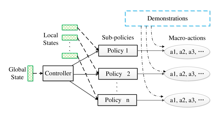
Our hierarchical architecture is illustrated in Fig. 1. There are two types of policies running in different timescales. The controller decides to choose a sub-policy based on current observation every long time interval, and the sub-policy picks a macro-action every short time interval.
For further illustration, we use to represent the controller. and is its state and action space. Similarly, assuming there is sub-policies in the pool, we use to represent them. The state and action space of th sub-policy is defined as and . is its reward function. Besides, we have a time interval K. It means that the controller chooses a sub-policy in every K time units and the chosen sub-policy makes a decision in every time unit. Now we can deeply go through the whole process.
At time , the controller gets its own global observation , and it will choose a sub-policy based on its state, like below:
| (5) |
Now the controller will wait for K time units and the th sub-policy begins to make its move. We assume its current time is and its local observation is , so it get the macro-action . After the th sub-policy doing the macro-action in the game, it will get the reward and its next local observation . The tuple will be stored in its local buffer for the future training. After K moves, it will return to the controller and wait for the next chance.
The high level controller gets the return of the chosen sub-policy and compute the reward of its action as follows:
| (6) |
Also, the controller will get its next global state and the tuple will be stored in its local buffer . Now the time is , and the controller will make a next choice based on its current global observation.
From above, we can see that there is some advantages in our hierarchical architecture. Firstly, each sub-policy and the high-level controller have different state space. We can see that the controller only needs the global information to make high-level decision. The global state space is a small part of all the state space . Also, a sub-policy responsible for combat is more focused on local state space related to battle. It can be seen that such a hierarchical structure can split the original huge state space into a plurality of subspaces corresponding to different policy networks. Secondly, the hierarchical structure can also split the tremendous action space . The sub-policies with different functions will have their own action space . Thirdly, the hierarchical architecture can effectively reduce the execution step size of the strategy. Since the control network calls a sub-network every fixed time interval , the total execution step size of the high-level network becomes step. The execution step size of sub-policies will also be reduced. Last but not least, the hierarchical architecture makes design of the reward functions easier. Different sub-policies may have different targets. Therefore, they can learn more quickly by their own suitable reward functions.
3.2 Generation of Macro-actions
In StarCraft, the original action space is tremendous. And human players always need to do a sequence of raw actions to achieve one simple purpose. For example, if we want to build a building in the game, we have to select a peasant, order it to build the building in the specific position, and make it come back after finish. The sequences of the raw actions for some simple purposes are more likely some fixed sequence stored in mind for our human players. So we instead generate a macro-action space which is obtained through data mining from trajectories of experts. The original action space is then replaced by the macro-action space . This will improve the learning efficiency and testing speed. The generation process of macro-actions is as follow:
-
•
Firstly, we collect some expert trajectories which are sequence of operations from game replays.
-
•
Secondly, we use a prefix-span (?) algorithm to mine the relationship of the each operation and combine the related operations to be a sequence of actions of which max length is and constructed a set which is defined as
-
•
Thirdly, we sort this set by .
-
•
Fourthly, we remove duplicated and meaningless ones, remain the top ones. Meaningless refers to the sequences like continuous selection or camera’s movement.
-
•
Finally, the reduced set are marked as newly generated macro-action space .
Using the macro-action space , our MDP problem is now reduced to a simple one, which is defined as:
| (7) |
Meanwhile, the MDP problem of each sub-policy is also reduced to new one:
| (8) |
Input: Number of sub-policies , time interval K, reward function , max episodes , max iteration steps , max game steps ,
3.3 Training Algorithm
The training process of our architecture is showed in Algorithm 1 and can be summarized as follows. Firstly we initialize the controller and sub-policies. Then we run the iteration of times and run the episode of times in each iteration. At the beginning of each iteration, we will clear all the replay buffers. In each episode, we collect the trajectories of the controller and sub-policies. At the end of each iteration, we use the replay buffers to update the parameters of the controller and sub-policies.
The update algorithm we use is PPO (?). Entropy’s loss was added to the PPO’s loss calculation to encourage exploration. Therefore, our loss formula is as follows:
| (9) |
where are the coefficients we need to tune, and S denotes an entropy bonus. is defined as follows:
| (10) |
| (11) |
where , is computed by a truncated version of generalized advantage estimation.
3.4 Reward Design
There are three types of rewards we explore in this paper. Win/Loss reward is a ternary 1 (win) / 0 (tie) / -1 (loss) received at the end of a game. Score reward is Blizzard score get from the game engine. Mixture reward is our designed reward function.
It’s hard for agent to learn the game using Win/Loss reward. Blizzard scores can be seen as dense reward. We will show that using this score as a reward can not help agent get more chances to win in the experiment section. We have designed reward functions for the sub-policies which combines dense reward and sparse reward. These rewards seem to be really effective for training, which will be shown in the experiment section.
3.5 Curriculum Learning
SC2 includes 10 difficult levels of built-in AI which are all crafted by rules and scripts. From level-1 to level-10, the built-in AI’s ability is constantly improving. Training in higher difficulty level gives less positive feedback, making it difficult for agent to learn from scratch. In this work, we trained our agent in lower difficulty level at first, then transferred the agent to higher difficulty level using the pre-trained model as the initial model, following the idea of curriculum learning.
However, when the pre-trained agent transfers to high difficulty levels, we find that if controller and all sub-policies are still updated at the same time, the training is sometimes unstable due to the mutual influence of different networks. In response to this situation, we have devised a strategy to update the controller and sub-policies alternatively. We found that this method can make the training more stable, and the winning rate for high difficulty levels can rise steadily.
4 Experiments
In this section, we present the experiment results on SC2LE. We first introduce the experiment settings including the hierarchical architecture and three combat models. Then the details of experiments are shown. If you want to get more information about experiment settings and implementation details such as features of state space or forms of macro actions, please refer to the appendix of our arxiv version 111https://arxiv.org/abs/1809.09095.
4.1 Setting
The setting of our architecture is as follow: controller selects one sub-policy every 8 seconds, and the sub-policy performs macro-actions every 1 second. In the setup, we have two sub-policies in the sub-policy pool. One sub-policy controls the construction of buildings and the production of units in the base, called base network. The other sub-policy is responsible for battle, called battle policy. This sub-policy has three different models, which are explained later.
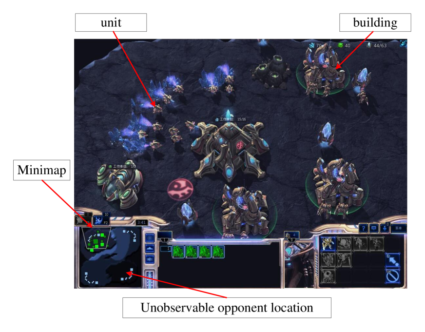
A full-length game of SC2 in the 1v1 mode is as follow: First, two players spawn on different random points in the map and accumulate resources. Second, they construct buildings and produce units. At last, they attack and destroy each other’s units and buildings. Fig. 2 shows a screenshot of the running game.
For simplicity, we set our agent’s race to Protoss and build-in AI’s race to Terran. But our algorithms could generalize to any race against any other race. The map we used is the 64x64 map simple64 on SC2LE. We set the maximum length of each game to minutes. Moreover, our agent does not open sub-mine, and only uses the two basic military units which are Zealot and Stalker.
In our setup, the battle policy has three different settings. These are explained below.
4.1.1 Combat rule
Combat rule is a simple battle policy, and there is only one action in combat rule model: attacking a sequence of fixed positions. Although the map is unobservable and the enemy’s position is unknown, the enemy always live around the mines. We only need to make our army attack the fixed positions around the mines. The attack action uses the built-in AI to do automatic move and attack. Thus the result of the attack action depends on the construction of the buildings and the production of the units. Only when the agent learns to better carry out building construction (for example, do not build redundant buildings, and build more pylons in time when supply is insufficient), it is possible for the agent to win.
4.1.2 Combat network
Though the simple combat rule model is effective, the combat process is slightly naive or rigid and may fail when moving to larger and more complex maps. Below we introduce a smarter attack approach which is called combat network. The output of the combat network consists of three actions and a position vector. These actions are: all attack a certain position, all retreat to a certain position, do nothing. Attack and move positions are specified by the position vector.
The combat network is constructed as a Convolution Neural Network (CNN). This CNN accepts feature maps of minimaps and screens which enabling it to know the information of the full map and the unit and building positions on the screen. Moreover, we use a simple strategy to decide the position of the camera. When the controller chooses the base sub-policy, the camera is moved to the location of agent’s base. When the controller chooses the battle sub-policy, the camera is moved to the location of army. The location of army can be chosen in two ways. The first is the center point of all combat units. The second is the center of the most injured unit. Since the injured unit indicated the occurrence of a recent battle, we found that the last setting was better in practice.
4.1.3 Mixture model
Although the combat network model can be trained well on high level of difficulty, it will occasionally miss some hidden enemy buildings. We can combine combat network with combat rule into a mixture model. When a certain value is predicted in the position vector of the combat network, the army’s attack position will become a series of fixed positions got by prior knowledge.
(a) Curriculum learning
(b) Module training
(c) Simultaneous unstable
(d) Alternative refine
(a) Hierarchy vs single
(b) Win/Loss vs handcrafted
(c) Score and win rate
(d) Impact of episode num
4.2 Comparison of Training Method
In the following, we will discuss our training processes from three aspects. Firstly, curriculum learning is the major way we use to train our agents against the enemy from low difficulty levels to high difficulty levels. Secondly, our hierarchical architecture can be used for module training, which is convenient for replacing sub-policies and refining some sub-policies while others fixed. Finally, our simultaneous training algorithm is sometimes unstable on high difficulty levels, so we instead use an alternative update strategy.
4.2.1 Effect of curriculum learning
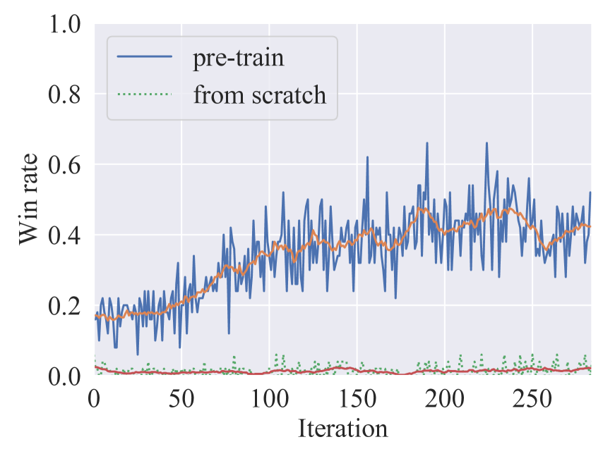
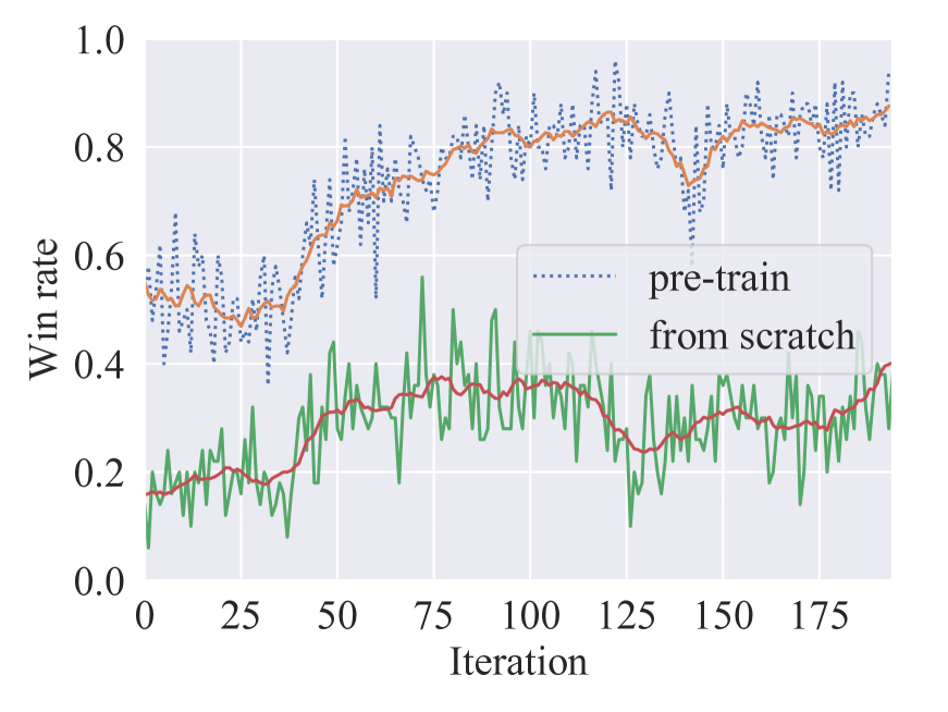
In all of our combat models, we firstly train them on low difficulty levels and then transfer them to high difficulty levels. This process follows the way of curriculum learning. We found that when training directly on high difficulty levels, the performance of our agent is difficult to improve. If we start training from low difficulty level and then use the low-difficulty’s model as the initial model to update, we could often get better results.
Fig. 3 (a) shows the comparison between training the pre-trained agent and training from scratch on difficulty level-7. These two agents are using combat network model, and the first agent has been trained on difficulty level-2 and difficulty level-5.
4.2.2 Effect of module training
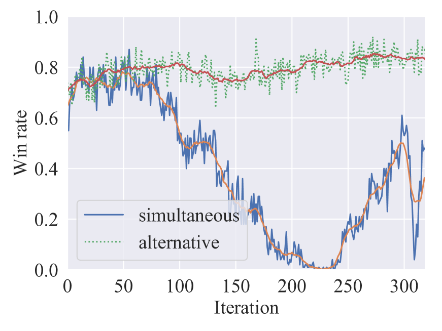
Since we are using a hierarchical architecture, we can easily replace sub-policies. While replacing a sub-policy, the parameters of the controller network and other sub-policies are retained, only the parameters of the newly replaced sub-policy are updated, which can accelerate learning. In the experiment, we have three types of combat strategies. If we have trained the simple combat rule model on high difficulty level, we can use the parameters of its controller network and base network for the other two combat models.
Fig. 3 (b) shows the comparison between training using pre-trained networks and training from scratch on difficulty level-2. These two agents are using combat network model, and the first agent uses the parameters of controller and base network which are from the combat rule model trained on difficulty level-7.
4.2.3 Effect of simultaneous updating
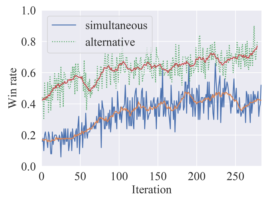
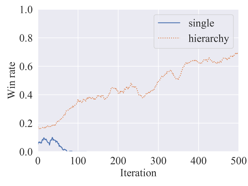
For the sample efficiency, in our training algorithm, we let all the networks of the hierarchical architecture collect their own data and then update at the same time. They are sometimes unstable. Because every network would see the other networks as the part of environment, and do not consider the changes of the others while updating. These unstable training rarely happened on lower difficulty levels, but can be seen on higher difficulty levels. We can use an alternate updating strategy to train the networks which can result in a steady improvement, but need more samples. We can also make the learning rate smaller which could also alleviate this problem. But the training process would be slower and sometimes hard to be improved.
Fig. 3 (c) shows the comparison between simultaneously updating and alternately updating on difficulty level-7. The agent uses combat rule model, and has been trained on difficulty level-2 and difficulty level-5.
Fig. 3 (d) also shows the comparison between simultaneously updating and alternately updating on difficulty level-7, but there are some differences. The agent uses combat network model and has been trained on difficulty level-2 and difficulty level-5. The learning rate is half smaller than Fig. 3 (c). The green line above is actually loading the trained model of the blue line below. In the experiment, we found that the blue line below could not be improved in the following training period, but the green line above could quickly improve after loading its model.
| Opponent’s Type | Non-cheating (Training) | Cheating (No-training) | ||||||||
| Difficulty Level | 1 | 2 | 3 | 4 | 5 | 6 | 7 | 8 | 9 | 10 |
| Combat Rule | 1 | 0.99 | 0.94 | 0.99 | 0.95 | 0.88 | 0.78 | 0.70 | 0.73 | 0.60 |
| Combat Network | 0.98 | 0.99 | 0.45 | 0.47 | 0.39 | 0.73 | 0.66 | 0.56 | 0.52 | 0.41 |
| Mixture Model | 1 | 1 | 0.99 | 0.97 | 1 | 0.90 | 0.93 | 0.74 | 0.71 | 0.43 |
4.3 Comparison of Combat Models
After training the three combat models on difficulty level-7, we perform evaluation for each of them. Each evaluation tests from difficulty level-1 to difficulty level-10. We run games in each difficulty level and report the winning rate. The result is shown in Table 1. In the difficulty level-1 to level-7, we found that the training agents have a very good performance. The built-in AI in difficulty level-8 to level-10 uses several different cheat techniques and select different strategies randomly. So the performances of them are unstable and with a bit of randomness. However, it can be seen that our trained agents still have a good performance on fighting against them. The videos of our agents can be searched by ”NJU-SC2-Bot” on Youtube.
4.3.1 Combat rule
The combat rule agent achieves good results in difficulty level-1 to difficulty level-5. We find that since agents can only use the two basic military units to fight, they are more inclined to use a fast attack fashion (called ’Rush’), which can guarantee the winning rate.
The behaviors of our learned agent is as follow. At the beginning, agents tend to produce more farmers to develop the economy. When the number of farmers is close to saturation, the agent will turn to produce soldiers. When the number of soldiers is sufficient, the agent will choose to attack. This layered progressive strategy is automatically learned through our reinforcement learning algorithm which illustrates the effectiveness of our approach.
4.3.2 Combat network
We also test the combat network model on all 10 difficulty levels. We found that although the combat network model achieves a good winning rate on difficulty level-7, the winning rates on several other difficulty levels are not high. It is worth noting that many results of the other levels of difficulty are tie. This means that the model of the combat network is more difficult to completely destroy the enemy (which means eliminating all enemy buildings). Some enemy’s buildings or units may be hidden somewhere. If we also see tie as victory, the winning rate of combat network is still high.
4.3.3 Mixture model
It can be found in Table 1 that the mixture model of combat network and combat rule has achieved best results in difficulty level 1-9. This can be explained as follow. The agent can not only choose the attacking area within the camera, but also can switch to a fierce attack on some certain points. This freedom can lead to a performance improvement which makes mixture model best in all three combat models.
4.4 Comparison of Settings
In this section we have three experiments to show the importance of hierarchy, design of reward and impact of hyper parameters.
4.4.1 Hierarchy vs non-hierarchy
As we use a hierarchical architecture, there is a common question which is that whether the SC2 problem can be handled by using a non-hierarchical architecture. In the paper of SC2LE, the learning effect of the original action and state space and non-hierarchical reinforcement learning algorithm has been given. It can be seen that the performance was not satisfied. Our architecture has two levels of abstraction. One is a reduction in the action space, which is done by macro-action. The other is a two-layer architecture that uses the controller to select sub-policies. We tested the effect of keeping the use of macro-actions without using the controller and sub-policies. This is called the single-policy architecture.
We were surprised to find that on low difficulty levels, the single-policy architecture can be almost as good as hierarchical architecture learning which means that macro-actions are effective for training a good agent. However, when moving to high level of difficulty, the final performance of the hierarchical architecture are significantly better than the single-policy architecture, as shown in Fig. 4 (a), which is trained on difficulty level-7. It can be explained that when the difficulty level is low, the difference between the hierarchical and non-hierarchical architecture is less obvious. When the difficulty of the problem continues to increase, the performance of the hierarchical model will be better than the performance of non-hierarchical model. Another reason for using hierarchy is modularity. Modularity facilitates the replacement of sub-policy. For example, if we need to replace battle sub-policy, we can still retain the parameters of other networks which speeds up training.
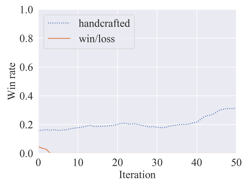
4.4.2 Outcome reward vs handcrafted reward
Win/Loss reward can achieve good results on low difficulty level like handcrafted reward. However, when training is on high difficulty level, we found that the performance of Win/Loss reward on hierarchical model is relatively poor as shown in Fig. 4 (b) in which the agent is using combat network model and trained on difficulty level-7.
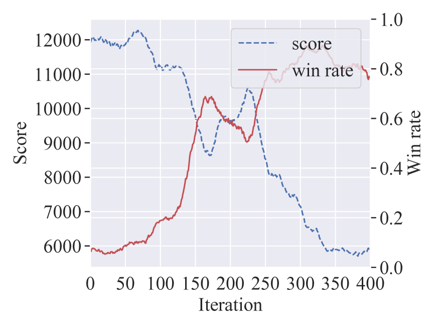
In SC2LE, it is mentioned that one can use Blizzard score as a reward. However, we found that Blizzard score and winning rate are sometimes not in a proportional relationship, especially on low difficulty levels. While the agent is trying to improve the score, it may ignore the attack chance on the enemy base and lose the best opportunity to win. This is shown in Fig. 4 (c) in which the agent is using combat network model and trained on difficulty level-2.
4.4.3 Influence of hyper-parameters
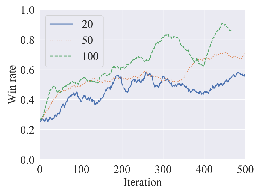
We have experimented with a variety of different parameters and found that the number of episodes in each iteration has some influence on the learning speed of the agent. When the number is small, the learning will be unstable and hard to converge. Improving the number of episodes can mitigate the problem. This effect is shown in Fig. 4 (d) in which the agent is using combat rule model and trained on difficulty level-2. Other parameters have little effect on training.
5 Conclusion
In this paper, we investigate a set of techniques of reinforcement learning for the full-length games in StarCraft II, including hierarchical policy training with extracted macro-actions, reward design, and curriculum design. With limited computation resource, we show that the combined approach achieves the state-of-the-art results beating the built-in AI. In the future, we will continue to explore more RL algorithms that can better solve large-scale problems.
References
- 1. D. Andre and S. J. Russell. State abstraction for programmable reinforcement learning agents. In Proceedings of the Eighteenth National Conference on Artificial Intelligence and Fourteenth Conference on Innovative Applications of Artificial Intelligence, July 28 - August 1, 2002, Edmonton, Alberta, Canada., pages 119–125, 2002.
- 2. P. Bacon, J. Harb, and D. Precup. The option-critic architecture. In Proceedings of the Thirty-First AAAI Conference on Artificial Intelligence, February 4-9, 2017, San Francisco, California, USA., pages 1726–1734, 2017.
- 3. T. G. Dietterich. Hierarchical reinforcement learning with the MAXQ value function decomposition. CoRR, cs.LG/9905014, 1999.
- 4. K. Frans, J. Ho, X. Chen, P. Abbeel, and J. Schulman. Meta learning shared hierarchies. CoRR, abs/1710.09767, 2017.
- 5. N. Justesen and S. Risi. Learning macromanagement in starcraft from replays using deep learning. pages 162–169, 2017.
- 6. S. Levine, C. Finn, T. Darrell, and P. Abbeel. End-to-end training of deep visuomotor policies. Journal of Machine Learning Research, 17:39:1–39:40, 2016.
- 7. V. Mnih, A. P. Badia, M. Mirza, A. Graves, T. P. Lillicrap, T. Harley, D. Silver, and K. Kavukcuoglu. Asynchronous methods for deep reinforcement learning. In Proceedings of the 33nd International Conference on Machine Learning, ICML 2016, New York City, NY, USA, June 19-24, 2016, pages 1928–1937, 2016.
- 8. V. Mnih, K. Kavukcuoglu, D. Silver, A. Graves, I. Antonoglou, D. Wierstra, and M. A. Riedmiller. Playing atari with deep reinforcement learning. CoRR, abs/1312.5602, 2013.
- 9. S. Ontañón, G. Synnaeve, A. Uriarte, F. Richoux, D. Churchill, and M. Preuss. A survey of real-time strategy game AI research and competition in starcraft. IEEE Trans. Comput. Intellig. and AI in Games, 5(4):293–311, 2013.
- 10. P. Peng, Q. Yuan, Y. Wen, Y. Yang, Z. Tang, H. Long, and J. Wang. Multiagent bidirectionally-coordinated nets for learning to play starcraft combat games. CoRR, abs/1703.10069, 2017.
- 11. J. Schulman, F. Wolski, P. Dhariwal, A. Radford, and O. Klimov. Proximal policy optimization algorithms. CoRR, abs/1707.06347, 2017.
- 12. S. Shalev-Shwartz, S. Shammah, and A. Shashua. Safe, multi-agent, reinforcement learning for autonomous driving. CoRR, abs/1610.03295, 2016.
- 13. D. Silver, A. Huang, C. J. Maddison, A. Guez, L. Sifre, G. van den Driessche, J. Schrittwieser, I. Antonoglou, V. Panneershelvam, M. Lanctot, S. Dieleman, D. Grewe, J. Nham, N. Kalchbrenner, I. Sutskever, T. P. Lillicrap, M. Leach, K. Kavukcuoglu, T. Graepel, and D. Hassabis. Mastering the game of go with deep neural networks and tree search. Nature, 529(7587):484–489, 2016.
- 14. D. Silver, J. Schrittwieser, K. Simonyan, I. Antonoglou, A. Huang, A. Guez, T. Hubert, L. Baker, M. Lai, A. Bolton, et al. Mastering the game of go without human knowledge. Nature, 550(7676):354, 2017.
- 15. P. Sun, X. Sun, L. Han, J. Xiong, Q. Wang, B. Li, Y. Zheng, J. Liu, Y. Liu, H. Liu, and T. Zhang. Tstarbots: Defeating the cheating level builtin AI in starcraft II in the full game. CoRR, abs/1809.07193, 2018.
- 16. R. Sutton and A. Barto. Introduction to reinforcement learning, volume 135. MIT press Cambridge, 1998.
- 17. R. S. Sutton, D. Precup, and S. P. Singh. Between mdps and semi-mdps: A framework for temporal abstraction in reinforcement learning. Artif. Intell., 112(1-2):181–211, 1999.
- 18. Y. Tian, Q. Gong, W. Shang, Y. Wu, and C. L. Zitnick. ELF: an extensive, lightweight and flexible research platform for real-time strategy games. In Advances in Neural Information Processing Systems 30: Annual Conference on Neural Information Processing Systems 2017, 4-9 December 2017, Long Beach, CA, USA, pages 2656–2666, 2017.
- 19. N. Usunier, G. Synnaeve, Z. Lin, and S. Chintala. Episodic exploration for deep deterministic policies: An application to starcraft micromanagement tasks. CoRR, abs/1609.02993, 2016.
- 20. A. S. Vezhnevets, S. Osindero, T. Schaul, N. Heess, M. Jaderberg, D. Silver, and K. Kavukcuoglu. Feudal networks for hierarchical reinforcement learning. In Proceedings of the 34th International Conference on Machine Learning, ICML 2017, Sydney, NSW, Australia, 6-11 August 2017, pages 3540–3549, 2017.
- 21. O. Vinyals, T. Ewalds, S. Bartunov, P. Georgiev, A. S. Vezhnevets, M. Yeo, A. Makhzani, H. Küttler, J. Agapiou, J. Schrittwieser, J. Quan, S. Gaffney, S. Petersen, K. Simonyan, T. Schaul, H. van Hasselt, D. Silver, T. P. Lillicrap, K. Calderone, P. Keet, A. Brunasso, D. Lawrence, A. Ekermo, J. Repp, and R. Tsing. Starcraft II: A new challenge for reinforcement learning. CoRR, abs/1708.04782, 2017.
- 22. X. Yan, J. Han, and R. Afshar. Clospan: Mining closed sequential patterns in large datasets. In Proceedings of the Third SIAM International Conference on Data Mining, San Francisco, CA, USA, May 1-3, 2003, pages 166–177, 2003.
- 23. V. F. Zambaldi, D. Raposo, A. Santoro, V. Bapst, Y. Li, I. Babuschkin, K. Tuyls, D. P. Reichert, T. P. Lillicrap, E. Lockhart, M. Shanahan, V. Langston, R. Pascanu, M. Botvinick, O. Vinyals, and P. Battaglia. Relational deep reinforcement learning. CoRR, abs/1806.01830, 2018.
Appendix A Appendix
A.1 State space
In our hierarchical architecture, the states has two types, which are the non-spatial features and the spatial features. The list of the non-spatial features is shown in Table 2. The content of the spatial features is based on Table 3. The controller only uses some of the non-spatial features as its global state. The base policy uses all the non-spatial features as its local state. The battle policy use both the non-spatial and spatial features as its local state.
| features | remarks |
|---|---|
| opponent.difficulty | from 1 to 10 |
| observation.game-loop | game time in frames |
| observation.player-common.minerals | minerals |
| observation.player-common.vespene | gas |
| observation.score.score-details.spent-minerals | mineral cost |
| observation.score.score-details.spent-vespene | gas cost |
| player-common.food-cap | max population |
| player-common.food-used | used population |
| player-common.food-army | population of army |
| player-common.food-workers | population of workers(probes) |
| player-common.army-count | counts of army |
| player-common.food-army / max(player-common.food-workers, 1) | rate of army on workers |
| num of army | the number of our army |
| num of probe, zealot, stalker, etc | multi-features |
| num of pylon, assimilator, gateway, cyber, etc | multi-features |
| score_cumulative | blizzard detailed score(multi-features) |
| * cost of pylon, assimilator, gateway, cyber, etc | multi-features |
| num of probe which are doing building actions | multi-features |
| * num of probe for mineral and the ideal num | multi-features |
| num of probe for gas and the ideal num | multi-features |
| num of the training probe, zealot, stalker | multi-features |
| features | post processing (map-width is set to 64) |
|---|---|
| observation(minimap)[height] | reshape(-1, map-width, map-width) / 255 |
| observation(minimap)[visibility] | reshape(-1, map-width, map-width) / 2 |
| observation(minimap)[camera] | reshape(-1, map-width, map-width) |
| observation(minimap)[relative] | reshape(-1, map-width, map-width) / 4 |
| observation(minimap)[selected] | reshape(-1, map-width, map-width) |
| observation(screen)[relative] | reshape(-1, map-width, map-width) / 4 |
| observation(screen)[selected] | reshape(-1, map-width, map-width) |
| observation(screen)[hitpoint-r] | reshape(-1, map-width, map-width) / 255 |
| observation(screen)[shield-r] | reshape(-1, map-width, map-width) / 255 |
| observation(screen)[density-a] | reshape(-1, map-width, map-width) / 255 |
A.2 Macro actions
The Macro actions are generated by using the PrefixSpan algorithm on our expert’s game replays. Table 4 shows the top 30 action sequences with the highest frequency of occurrence. As we can see, the first action of the action sequences is necessarily the selection action. In addition, many actions in the action sequences are about screen movement. This operation produces different effects depending on the target of execution. Therefore, it is not helpful for building macro actions and can be discarded. When we have dropped some duplicate or meaningless action sequences, we can construct a collection of macro actions with the remaining ones. It should be noted that since macro actions are not code, we need to ”translate” them into specific code. These codes need to be carefully written to ensure that they perform the sequence of operations in macro actions.
| action sequences | frequency |
|---|---|
| select-point(unit name: Protoss.Probe) Harvest-Gather-Probe-screen | 2711 |
| select-point(unit name: Protoss.Probe) Smart-screen | 2253 |
| select-point(unit name: Protoss.Nexus) Train-Probe-quick | 1421 |
| select-point(unit name: Protoss.Probe) Build-Pylon-screen | 1298 |
| select-point(unit name: Protoss.Nexus) Smart-screen | 1030 |
| select-point(unit name: Protoss.Nexus) select-army | 968 |
| select-point(unit name: Protoss.Probe) Build-Gateway-screen | 814 |
| select-point(unit name: Protoss.Gateway) Train-Zealot-quick | 762 |
| select-point(unit name: Protoss.Probe) Build-Pylon-screen Harvest-Gather-Probe-screen | 659 |
| select-point(unit name: Protoss.Gateway) Train-Stalker-quick | 621 |
| select-point(unit name: Protoss.Nexus) select-army Attack-Attack-screen | 581 |
| select-point(unit name: Protoss.Probe) select-army | 574 |
| select-point(unit name: Protoss.Nexus) Train-Zealot-quick | 536 |
| select-point(unit name: Protoss.Gateway) select-army | 467 |
| select-point(unit name: Protoss.Probe) Build-Gateway-screen Harvest-Gather-Probe-screen | 466 |
| select-point(unit name: Protoss.Nexus) Train-Stalker-quick | 325 |
| select-point(unit name: Protoss.Gateway) Smart-screen | 300 |
| select-point(unit name: Protoss.Gateway) select-army Attack-Attack-screen | 284 |
| select-point(unit name: Protoss.Probe) Attack-Attack-screen | 260 |
| select-point(unit name: Protoss.Probe) Build-Pylon-screen Smart-screen | 258 |
| select-point(unit name: Protoss.Probe) select-army Attack-Attack-screen | 254 |
| select-point(unit name: Protoss.Probe) Build-Assimilator-screen | 253 |
| select-point(unit name: Protoss.Probe) Train-Zealot-quick | 243 |
| select-point(unit name: Protoss.Gateway) Cancel-BuildInProgress-quick | 209 |
| select-point(unit name: Protoss.Probe) Smart-screen Build-Pylon-screen | 194 |
| select-point(unit name: Protoss.Probe) Build-CyberneticsCore-screen | 182 |
| select-point(unit name: Protoss.Probe) Smart-screen select-army | 166 |
| select-point(unit name: Protoss.Probe) Smart-screen Harvest-Gather-Probe-screen | 164 |
| select-point(unit name: Protoss.Probe) Smart-screen Build-Gateway-screen | 147 |
| select-point(unit name: Protoss.Probe) Harvest-Gather-Probe-screen select-army | 147 |
A.3 Reward Function
The reward function has two type. One is dense or instant reward, which can be got after every action. The other is sparse or final reward, which only can be got in the terminal state. The controller and the sub-policies use the same final reward, which is the win/lose and the time penalty. For each sub-policy, the dense or instant reward is different. In our best version, the instant rewards depend on the number of the units and structures. For example, the number of probe, pylon, army and so on. There is also another version which performed slightly worse than before. It uses the Blizzard detailed score as the reward. More specifically, the base policy use the worker idle time, the production idle time, total value unit and total value structures as its instant reward. The battle policy use the killed value units and killed value structures as its reward. The instant reward for the controller is the cumulative sum of the chosen sub-policy’s instant reward in the time interval.
A.4 Training Setting
In the experiment, we used a machine with 4 GPUs and 48 CPUs. There were 10 workers and each worker had 5 threads. Every thread was corresponding to a SC2 environment. In other words, There were 50 running environments at the same time. They all shared the global hierarchical architecture and also the parameters of networks. Since we used PPO algorithm for the training, our distributed system was simultaneous. In each iteration, we made the workers run 100 full-length games of SC2 and each worker would collect the data from 10 episodes. It would takes about 4 minutes. When all the workers had finished collecting the data, each worker would compute the gradients on its own. Finally, all the gradients from the wokers would be gathered and used to update the global hierarchical architecture.
A.5 Building Location
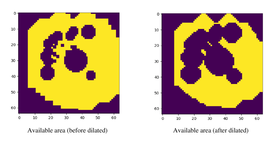
It is worth noting that the construction of buildings had to be given a location. There are mainly three ways to get it. The first one is by learning, the second one is by heuristic algorithms or human knowledge, and the third one is by random. The method by learning or human knowledge is too expensive, and most locations had little influence on our experiment. Therefore, after some trials, we chosed the location by random.
However, random selection without restriction would cause conflicts with other buildings or units, since the building that was going to build havd its collision volumes. We selected a commonly used dilation algorithm in the field of image processing research to solve this problem. This method would reduce the available area depended on the size of the building which was going to build. The success rate of the construction operation on the reduced area was greatly improved. In Fig. 5, the left figure is an original available map, and the right one is a reduced map after the dilating operator. It can be seen that the area that can be constructed (yellow) becomes smaller after dilation algorithm. Protoss is a relatively special race that requires the supply of power in addition to the need for open space. Therefore, when building a building other than Pylon, the area has to be logically AND with a power mask screen to obtain the area map that can be finally constructed.
