Axiomatic construction of quantum Langevin equations

Rúbia Araújo^a,b, Sascha Wald^c, and Malte Henkel^a,d

^aLaboratoire de Physique et Chimie Théoriques (CNRS UMR 7019),

Université de Lorraine Nancy, B.P. 70239, F – 54506 Vandœuvre lès Nancy Cedex, France

^bDepartamento de Matemática, Universidade Federal de Pernambuco, Avenida Professor Moraes Rego, 1235 - Cidade Universitária, CEP 50740-560, Recife - PE, Brazil

^cSISSA - International School for Advanced Studies and INFN, via Bonomea 265,

I – 34136 Trieste, Italia

^dCentro de Física Teórica e Computacional, Universidade de Lisboa,

P–1749-016 Lisboa, Portugal

A phenomenological construction of quantum Langevin equations, based on the physical criteria of (i) the canonical equal-time commutators, (ii) the Kubo formula, (iii) the virial theorem and (iv) the quantum fluctuation-dissipation theorem is presented. The case of a single harmonic oscillator coupled to a large external bath is analysed in detail. This allows to distinguish a markovian semi-classical approach, due to Bedeaux and Mazur, from a non-markovian full quantum approach, due to to Ford, Kac and Mazur. The quantum-fluctuation-dissipation theorem is seen to be incompatible with a markovian dynamics. Possible applications to the quantum spherical model are discussed.
 

PACS numbers: 05.30-d, 67.10.Fj, 05.10.Gg, 05.30.Rt

1 Introduction

The description of quantum-mechanical many-body problems far from equilibrium presents conceptual difficulties which go beyond those present in classical systems [10, 22, 15, 31, 71, 63]. In particular, while for classical systems either a master equation or a Langevin equation can readily be written down, this is far from obvious for quantum systems. To obtain at least formally a set of equations of motion, whose properties could then be studied, requires careful analysis of the quantum system. While this problem is quite well understood for isolated systems, for open quantum systems even the correct formulation of the problem appears to be not completely settled.

In classical non-equilibrium statistical mechanics, writing down a Langevin equation is a standard, well-established approach for the description of the dissipative relaxation of any classical system towards its stationary (or equilibrium) state. However, its most straightforward extension to quantum systems does not work satisfactorily. We recall this difficulty using the example of a single harmonic oscillator, see e.g. [11, 10]. If $s=s(t)$ denotes the magnetic ‘spin’ variable and $p=p(t)$ the canonically conjugated momentum, the ‘natural Langevin equation’ would read

$$\partial_{t}s=\frac{1}{m}p\;\;,\;\;\partial_{t}p=-m\omega^{2}s-\lambda p+\eta$$ (1.1)

where $m$ is the mass and $\omega$ the natural angular frequency of the oscillator. The coupling of the oscillator to an external heat bath is described by additional forces. These are (i) a dissipative force (assumed ohmic for simplicity) parametrised by the dissipation rate $\lambda$ and (ii) a random force, which is modelled by a centred gaussian noise $\eta$. Consider the equal-time commutator $c(t)=\langle[s(t),p(t)]\rangle$, where initially $c(0)={\rm i}\hbar$. If $\langle[s(t),\eta(t)]\rangle=0$, eq. (1.1) implies the decay $c(t)={\rm i}\hbar\,{\rm e}^{-t/\lambda}$ [11]. Such a behaviour is inconsistent with the one of a genuine quantum system, even at temperature $T=0$. On the other hand, eq. (1.1) does furnish an adequate treatment for classical dynamics. The problem of finding consistent quantum Langevin equations (qles) has been intensively discussed, see [31, 71] for detailed reviews and refs. therein.

Bedeaux and Mazur [4, 5] suggested a different quantum Langevin equation. For the case of a single quantum harmonic oscillator (qho), their proposal reads ($m,\omega,\lambda$ are positive constants)

$$\partial_{t}s=\frac{1}{m}p+\eta_{s}\;\;,\;\;\partial_{t}p=-m\omega^{2}s-\lambda p+\eta_{p}$$ (1.2)

where the two distinct noises $\eta_{p},\eta_{s}$ are assumed to be centred Gaussians, with the second moments

$$\left\langle\eta_{p}(t)\eta_{p}(t^{\prime})\right\rangle =\lambda m\hbar\omega\coth\left(\hbar\omega/2k_{\rm B}T\right)\,\delta(t-t^{\prime})$$ (1.3a)

$$\left\langle\eta_{s}(t)\eta_{p}(t^{\prime})\right\rangle =-\left\langle\eta_{p}(t)\eta_{s}(t^{\prime})\right\rangle=\frac{1}{2}\,{\rm i}\hbar\lambda\,\delta(t-t^{\prime})$$ (1.3b)

$$\left\langle\eta_{s}(t)\eta_{s}(t^{\prime})\right\rangle =0$$ (1.3c)

and wherein the order of the operator noises $\eta_{s},\eta_{p}$ is essential. Also, $T$ is the temperature of the bath and $\delta$ denotes the Dirac distribution. Clearly, eqs. (1.2,1.3) describe a system with the Markov property. This approach was based on an analysis of the master equation of the density matrix $\rho$, viz. $\hbar\partial_{t}\rho=-{\rm i}[H,\rho]+\hbar{\cal L}\delta S/\delta\rho$, where $S$ is the thermodynamic entropy. The properties of the super-operator ${\cal L}$ are constrained by (i) the hermiticity of the thermodynamic force $\delta S/\delta\rho$, (ii) the conservation of probability, i.e. $\operatorname{tr}\left(\rho\right)=1$ for all times $t\geq 0$ and (iii) the Onsager relations. From this, they deduced the following equation of motion for time-dependent averages of an operator $A$ [4, 5]

$$\frac{{\rm d}}{{\rm d}t}\left(\langle A\rangle(t)-\langle A\rangle_{\rm eq}\right)=\operatorname{tr}\left(\frac{{\rm d}A}{{\rm d}t}\,\delta\rho\right)=\operatorname{tr}\left(\left(\frac{{\rm i}}{\hbar}\left[H,A\right]+\lambda A-\frac{{\rm i}\lambda}{\hbar}\left[Ap,x\right]\right)\delta\rho\right)\ ,$$ (1.4)

where $\delta\rho=\rho-\rho_{\rm eq}$ and $\rho_{\rm eq}$ denotes the equilibrium density matrix. They also worked out all two-time Green’s functions of spin and momentum in the stationary state from (1.4) and verified that a direct solution of (1.2) reproduces the noise correlators (1.3).

Figure 1: Schematic LRC circuit.

For illustration, we briefly mention two possible applications of the equations (1.2). (a) First, consider a $LRC$ circuit, see fig. 1. According to Kirchhoff’s law, the total voltage is $U(t)=U_{R}+U_{L}+U_{C}$ and one may set $U_{R}=RI$ and $U_{L}=L\dot{I}$, where $I=I(t)$ is the current. The coupling to an external bath is described by noise terms. The combined noises of the resistor $R$ and the coil $L$ are taken into account by setting $U(t)=L\eta_{U}$. For the capacitor $C$, the temporally rough changes in the voltage, sometimes referred to as ‘$kTC$-noise’ [41], are described by $\dot{U}_{C}=\frac{1}{C}I+\eta_{I}$. Herein, one will consider $\frac{1}{C}I(t)$ as the contribution to $\dot{U}_{C}$ which depends smoothly on the time $t$, whereas the noise $\eta_{I}(t)$ describes the rough contribution. Such a ‘reset noise’ arises from the thermodynamic fluctuations of the amount of charge on the capacitor [3, 45, 59, 30, 65]. It is the dominant noise on sufficiently small capacitors and can be the limiting noise, e.g. in image sensors [45, 59]. Combining the above equations leads to the system

$$\partial_{t}U_{C}=\frac{1}{C}I+\eta_{I}\;\;,\;\;\partial_{t}I=-\frac{R}{L}I-\frac{1}{L}U_{C}+\eta_{U}$$ (1.5)

which is identical to (1.2), upon the correspondences $s\leftrightarrow U_{C}$, $p\leftrightarrow I$ and $\eta_{s}\leftrightarrow\eta_{I}$, $\eta_{p}\leftrightarrow\eta_{U}$. While most of the literature discusses classical fluctuations, quantum fluctuations, as we shall discuss in this work, will become important for analysing noisy nano-electronic circuits [30, 12, 14]. Their discussion may require to trace precisely the several potential sources of noise present.

(b) Second, the oscillator (1.2) also arises in model descriptions of the working of the inner ear of vertebrates [48, 18]. It is a known biological fact that the vertebrate ear not only admits but also emits sound, the so-called spontaneous otoacoustic emissions. Such an active process in the inner ear is well-described by models near to an oscillatory instability which occurs on the onset of a Hopf bifurcation [48]. Specialised mechanoreceptors, i.e. bundles of hair cells, provide the work required of such active processes. Indeed, eq. (1.2) is a special case of the most simple of such models, where $s$ describes the hair-bundle position and $p$ the force exerted by the active process. The two noises $\eta_{s},\eta_{p}$, respectively, describe the effects of fluctuations on the bundle position and the active process, respectively [48, 18].

How can one decide whether a given system of equations of motion, or a master equation, can describe a genuine quantum system ? Using the proposal (1.2,1.3) of Bedeaux and Mazur as a phenomenological device, we formulate the following minimal criteria for a reasonable description of quantum dynamics:

1. the (averaged) canonical equal-time commutators $\bigl{\langle}[s_{n}(t),p_{m}(t)]\bigr{\rangle}={\rm i}\hbar\,\delta_{n,m}$ should be kept for all times $t>0$, if initially obeyed.

2. the Kubo formulæ of linear response theory should be reproduced (we shall recall the precise definition in section 2).

As we shall see, these requirements will be sufficient to fix the commutators between the two noises $\eta_{s},\eta_{p}$. In addition, one must require that

1. the virial theorem should be reproduced (it is valid in both classical and quantum mechanics and is used to analyse strongly interacting many-body systems at ‘thermal’ equilibrium. Important examples arise in astrophysics and cosmology for self-gravitating systems, where commonly ‘virialisation’ and ‘equilibration’ are treated as synonyms [17, 38, 60, 49]).

2. the quantum fluctuation-dissipation theorem (qfdt) will be an essential characteristic of quantum equilibrium states. It has been recognised since a long time that the qfdt is the key requirement for a stationary state being a quantum equilibrium state, in order to be consistent with the second fundamental theorem of quantum thermodynamics [37, 28].

   Indeed, it has been understood recently that the qfdt is a consequence of the invariance of the Keldysh path integral under a combined time-reversal and Kubo-Martin-Schwinger transformation [62, 2]. Moving away from the quantum equilibrium state will break this symmetry and the qfdt will cease to be valid. Therefore, the confirmation of the qfdt will serve to distinguish quantum equilibrium states from any other type of stationary state.

These two conditions will fix the anti-commutators of the two noises $\eta_{s},\eta_{p}$. Of course, a discussion must include the question whether all these requirements can be satisfied simultaneously.

Here, we wish to explore which kinds of dynamics are compatible with these criteria. In any case, a microscopic derivation of a ‘quantum Langevin equation’ which describes thermalisation should obey a series of physically reasonable consistency requirements, which we take to be the four criteria (A,B,C,D). We shall proceed in several steps. In section 2, we shall re-consider the case of a single harmonic oscillator, described by (1.2) following the suggestion of [4, 5] of including two noises $\eta_{s},\eta_{p}$, but we shall also include the effect of initial conditions. Proceeding from the exact solution of (1.2), we shall show that the phenomenological criteria (A,B,C) formulated above provide increasing constraints on the two noises $\eta_{s},\eta_{p}$ such that the combination of all three criteria finally reproduces the proposal (1.3) of Bedeaux and Mazur. On the other hand, the requirement (D) of the qfdt only holds true in the $\hbar\to 0$ limit. In section 3, a proposal for a quantum Langevin equation of the damped harmonic oscillator, with two noises $\eta_{s},\eta_{p}$, will be presented such that all four criteria (A,B,C,D) will be obeyed. In addition, the noise correlators are independent of the model parameters $m,\omega$ and only contain the damping constant $\lambda$. Also, the noise correlators are non-markovian. A possible explicit form is

$$\left\langle\eta_{s}(t)\eta_{s}(t^{\prime})\right\rangle =\left\langle\eta_{p}(t)\eta_{p}(t^{\prime})\right\rangle=0$$ (1.6a)

$$\left\langle\eta_{s}(t)\eta_{p}(t^{\prime})\right\rangle =-\left\langle\eta_{p}(t)\eta_{s}(t^{\prime})\right\rangle=\frac{1}{2}\,{\rm i}\hbar\lambda\,\delta(t-t^{\prime})+\frac{1}{2}\lambda k_{\rm B}T\coth\left(\frac{\pi k_{\rm B}T}{\hbar}(t-t^{\prime})\right)$$ (1.6b)

where the order of the operators is essential. We shall see that the non-markovianity is a direct consequence of the qfdt. Eqs. (1.2,1.6) state our proposal for the quantum Langevin equation of the damped quantum harmonic oscillator, in the special case of ohmic damping. Since the noise correlators do not depend on the parameters $m,\omega$ of the model we used as a scaffold to derive them, they should be generic and applicable in wider contexts. We shall also show that the qles (1.2,1.6) are equivalent to the second-order Ford-Kac-Mazur (fkm) quantum Langevin equation [25, 26, 27, 31, 71] of a particle in an external potential.

We must add that eqs. (1.6) are not the only solution to the criteria (A,B,C,D). Rather, we shall see that the most general solution can be expressed by two anti-symmetric functions $\psi(t),\chi(t)$ and two symmetric functions $\alpha(t),\beta(t)$ which also depend on the parameters $m,\omega$.

In section 4, we shall illustrate a few simple consequences of the noise correlators (1.6). The Langevin equations of the quantum harmonic oscillator can be re-interpreted as the qle of the modes of the quantum spherical model in $d$ spatial dimensions. The non-trivial physics (i.e. distinct from mean-field theory) of this model follows from the coupling of these modes by the so-called spherical constraint, which is included into the qle via a time-dependent Lagrange multiplier. The equilibrium critical behaviour of the quantum spherical model is well-known [51, 40, 50, 66, 52, 58, 7, 8, 67]: while for finite temperatures $T>0$, the critical behaviour is the same as for the classical spherical model [6, 44], at temperature $T=0$ there is a quantum critical point in the same universality class as the $(d+1)$-dimensional classical spherical model [42]. The time-dependent non-equilibrium classical system has also been very thoroughly analysed, see e.g. [57, 13, 33, 29, 54, 15, 39, 21, 20]. The non-equilibrium behaviour of isolated quantum or classical spherical models was studied recently [61, 47, 16]. The long-time dynamics of a disordered quantum spherical model was analysed in the mean-field limit [56]. The quantum dynamical behaviour of the open quantum spherical model quenched to temperature $T=0$ as described by a Lindblad equation was recently studied [68, 69, 70, 64] and it was shown that for quantum quenches deep into the ordered state, the long-time behaviour of several averages becomes independent of the coupling to the bath. We shall outline how the explicit solution of the quantum spherical dynamics can be considerably simplified in the long-time limit via a scaling argument. This can be done for both the Bedeaux-Mazur noise correlators (1.3) as well as for the quantum noise correlators (1.6). The qualitative difference of quantum and classical correlators will also be illustrated for the qho. We have therefore explicitly formulated the qle of the quantum spherical model. However, finding the late-time solutions explicitly is still technically demanding and will be left to future work. We conclude in section 5. Several appendices give further background and calculational details.

2 Semi-classical dissipative harmonic oscillator

The quantum Langevin equations (1.2) are characterised by the two noises $\eta_{s}(t)$ and $\eta_{p}(t)$. In addition, we shall have to characterise the fluctuations of the initial state. We shall apply the criteria formulated in section 1 to constrain their possible form. From now on, we set $k_{\rm B}=1$.

2.1 Formal solution

The first step of the solution of eq. (1.2) is to re-write the homogeneous part in matrix form

$$\partial_{t}\left(\mbox{${\begin{array}[]{c}s\\ p\end{array}}$}\right)=\left(\mbox{${\begin{array}[]{cc}0&1/m\\ -m\omega^{2}&-\lambda\end{array}}$}\right)\left(\mbox{${\begin{array}[]{c}s\\ p\end{array}}$}\right)=-\Lambda\left(\mbox{${\begin{array}[]{c}s\\ p\end{array}}$}\right)$$ (2.1)

The eigenvalues of the matrix $\Lambda$ are

$$\Lambda_{\pm}=\frac{\lambda}{2}\pm\sqrt{\frac{\lambda^{2}}{4}-\omega^{2}\,}$$ (2.2)

and they obey the following properties: if $0<|\omega|<\lambda/2$, then $\Lambda_{+}>\Lambda_{-}>0$. If $|\omega|>\lambda/2>0$, then $\Lambda_{-}^{*}=\Lambda_{+}$ and ${\rm Re\ }\Lambda_{\pm}=\lambda/2>0$.

The homogeneous solution implies the following ansatz

$$s(t)=s_{+}(t){\rm e}^{-\Lambda_{+}t}+s_{-}(t)e^{-\Lambda_{-}t}\;\;,\;\;p(t)=p_{+}(t){\rm e}^{-\Lambda_{+}t}+p_{-}(t)e^{-\Lambda_{-}t}$$ (2.3)

in order to solve eq. (1.2) with the method of variation of constants. Two of the four amplitudes ($s_{\pm},p_{\pm}$) in the ansatz can be still chosen freely. Our choice is

$$p_{\pm}(t)=-m\Lambda_{\pm}s_{\pm}(t)$$ (2.4)

Now, we reinsert the ansatz (2.3) into the eqs. (1.2), and use the conditions (2.2,2.4). This leads to the simplified system (the dots denote the derivative with respect to time)

$$\dot{s}_{+}(t){\rm e}^{-\Lambda_{+}t}+\dot{s}_{-}(t){\rm e}^{-\Lambda_{-}t}=\eta_{s}(t)\;\;,\;\;-\Lambda_{+}\dot{s}_{+}(t){\rm e}^{-\Lambda_{+}t}-\Lambda_{-}\dot{s}_{-}(t){\rm e}^{-\Lambda_{-}t}=\frac{1}{m}\eta_{p}(t)$$ (2.5)

which can be separated as follows (throughout, we assume $|\omega|\neq\lambda/2$)

$$\dot{s}_{+}(t)=-\frac{\exp(\Lambda_{+}t)}{\Lambda_{+}-\Lambda_{-}}\left(\frac{\eta_{p}}{m}+\Lambda_{-}\eta_{s}\right)\;\;,\;\;\dot{s}_{-}(t)=\frac{\exp(\Lambda_{-}t)}{\Lambda_{+}-\Lambda_{-}}\left(\frac{\eta_{p}}{m}+\Lambda_{+}\eta_{s}\right)$$ (2.6)

Their immediate integration then gives the formal exact solution of (1.2)

$$s(t) =s_{+}(0){\rm e}^{-\Lambda_{+}t}+s_{-}(0){\rm e}^{-\Lambda_{-}t}$$

$$-\frac{1}{\Lambda_{+}-\Lambda_{-}}\int_{0}^{t}\!{\rm d}\tau\>{\rm e}^{-\Lambda_{+}(t-\tau)}\left[\frac{\eta_{p}(\tau)}{m}+\Lambda_{-}\eta_{s}(\tau)\right]+\frac{1}{\Lambda_{+}-\Lambda_{-}}\int_{0}^{t}\!{\rm d}\tau\>{\rm e}^{-\Lambda_{-}(t-\tau)}\left[\frac{\eta_{p}(\tau)}{m}+\Lambda_{+}\eta_{s}(\tau)\right]$$ (2.7a)

$$p(t) =-m\Lambda_{+}s_{+}(0){\rm e}^{-\Lambda_{+}t}-m\Lambda_{-}s_{-}(0){\rm e}^{-\Lambda_{-}t}$$

$$+\frac{m\Lambda_{+}}{\Lambda_{+}-\Lambda_{-}}\int_{0}^{t}\!{\rm d}\tau\>{\rm e}^{-\Lambda_{+}(t-\tau)}\left[\frac{\eta_{p}(\tau)}{m}+\Lambda_{-}\eta_{s}(\tau)\right]-\frac{m\Lambda_{-}}{\Lambda_{+}-\Lambda_{-}}\int_{0}^{t}\!{\rm d}\tau\>{\rm e}^{-\Lambda_{-}(t-\tau)}\left[\frac{\eta_{p}(\tau)}{m}+\Lambda_{+}\eta_{s}(\tau)\right]$$ (2.7b)

Eqs. (2.7) will be the basis of all subsequent calculations.

2.2 Equal-time commutator

While the amplitudes $s_{\pm}(0)$ characterise the fluctuations of the initial state, the fluctuations of the bath are described by $\eta_{s}(t)$ and $\eta_{p}(t)$. We assume that these two types of fluctuations are independent of each other and therefore that on average

$$\left\langle\left[s_{\pm}(0),\eta_{a}(t)\right]\right\rangle=0\;\;,\;\;\left\langle\left[\eta_{a}(t),\eta_{a}(t^{\prime})\right]\right\rangle=0$$ (2.8)

where $a=s,p$ labels the two noises. The second relation asserts that noises of the same kind (either for the spin or for the momentum) should commute. It remains to fix the commutator $\left\langle\left[s_{+}(0),s_{-}(0)\right]\right\rangle$ and we also consider the mixed commutator

$$\left\langle\left[\eta_{s}(t),\eta_{p}(t^{\prime})\right]\right\rangle=\kappa\,\delta(t-t^{\prime})$$ (2.9)

where the constant $\kappa$ is to be found. Here, we shall use the $\delta$-distribution in order to simplify the calculations. The physical argument behind is that we observe the system’s dynamics on time-scales large with respect to any correlation times in the bath. If that assumption should not be justified, a different bath correlation kernel must be used (in that case $\kappa\delta(t-t^{\prime})$ would become a time-dependent function $\kappa(t-t^{\prime})$). We shall not explore that possibility in this section, however.

Using the exact solution (2.7), the spin-momentum commutator is readily worked out

$$\left\langle\big{[}s(t),p(t^{\prime})\big{]}\right\rangle =-\frac{\kappa}{(\Lambda_{+}-\Lambda_{-})(\Lambda_{+}+\Lambda_{-})}\bigg{(}\Lambda_{+}{\rm e}^{-\Lambda_{-}|t-t^{\prime}|}-\Lambda_{-}{\rm e}^{-\Lambda_{+}|t-t^{\prime}|}\bigg{)}$$ (2.10)

$$+m\bigg{(}\Lambda_{+}{\rm e}^{-\Lambda_{-}t-\Lambda_{+}t^{\prime}}-\Lambda_{-}{\rm e}^{-\Lambda_{+}t-\Lambda_{-}t^{\prime}}\bigg{)}\bigg{(}\left\langle\big{[}s_{+}(0),s_{-}(0)\big{]}\right\rangle-\frac{\kappa/m}{(\Lambda_{+}-\Lambda_{-})(\Lambda_{+}+\Lambda_{-})}\bigg{)}$$

We identify two contributions: for large enough times, only the stationary part will contribute (the first line in (2.10)), but there is also a non-stationary part, given by the second line of (2.10). The stationarity of the spin-momentum commutator can be achieved by requiring the following initial condition

$$\left\langle\left[s_{+}(0),s_{-}(0)\right]\right\rangle=\frac{\kappa/m}{(\Lambda_{+}-\Lambda_{-})(\Lambda_{+}+\Lambda_{-})}$$ (2.11)

The sought canonical commutator is obtained from the remaining stationary commutator $\left\langle\left[s(t),p(t^{\prime})\right]\right\rangle$ when we also set $t=t^{\prime}$. We read off

$$\left\langle\left[s(t),p(t)\right]\right\rangle=\frac{\kappa}{\lambda}\stackrel{{\scriptstyle!}}{{=}}{\rm i}\hbar$$ (2.12)

so that we can identify

$$\kappa={\rm i}\lambda\hbar\;\;,\;\;\left\langle\left[\eta_{s}(t),\eta_{p}(t^{\prime})\right]\right\rangle={\rm i}\lambda\hbar\,\delta(t-t^{\prime})$$ (2.13)

The second of these reproduces eq. (1.3b) as proposed in [4].

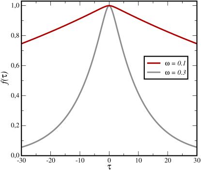
Figure 2: Time-dependence of the normalised commutator $f(\tau)=\langle[s(\tau),p(0)]\rangle/({\rm i}\hbar)$, over against the time difference $\tau$, for $\lambda=1$ and two values of $\omega$.

On the other hand, for different times $t\neq t^{\prime}$, the canonical spin-momentum commutator is not kept, but only depends on the time difference $\tau=t-t^{\prime}$. The functional form of the two-time commutator is illustrated in figure 2. For increasing values of $\omega$ (but still small enough that $\Lambda_{\pm}$ are real), the peak at $\tau=0$ becomes more sharp but there is no simple and model-independent argument to predict this form.

2.3 Linear responses

As a preparation for the discussion of the Kubo formula and the fluctuation-dissipation theorem (fdt), we compute responses of the average spin and momentum to an external magnetic perturbation. The hamiltonian reads $H=\frac{p^{2}}{2m}+\frac{m\omega^{2}}{2}s^{2}-hs$. The quantum equations of motion of the closed system are $\dot{p}=\frac{{\rm i}}{\hbar}[H,p]$ and $\dot{s}=\frac{{\rm i}}{\hbar}[H,s]$, where the equal-time canonical commutator $[s,p]={\rm i}\hbar$ is to be used. Adding to these the damping and noise terms of the open system, the full equations of motion become now

$$\dot{s}=\frac{1}{m}p+\eta_{s}\;\;,\;\;\dot{p}=-m\omega^{2}s+h-\lambda p+\eta_{p}$$ (2.14)

The linear responses of the spin $s$ and of the momentum $p$ are defined as

$$R^{(s)}(t,t^{\prime}):=\left.\frac{\delta\langle s(t)\rangle}{\delta h(t^{\prime})}\right|_{h=0}\;\;,\;\;Q^{(p)}(t,t^{\prime}):=\left.\frac{\delta\langle p(t)\rangle}{\delta h(t^{\prime})}\right|_{h=0}$$ (2.15)

They obey the equations

$$\partial_{t}R^{(s)}(t,t^{\prime})=\frac{1}{m}Q^{(p)}(t,t^{\prime})\;\;,\;\;\partial_{t}Q^{(p)}(t,t^{\prime})=-m\omega^{2}R^{(s)}(t,t^{\prime})-\lambda Q^{(p)}(t,t^{\prime})+\delta(t-t^{\prime})$$ (2.16)

Writing $\mathscr{R}(t-t^{\prime},t^{\prime})=R^{(s)}(t,t^{\prime})$ and denoting $\tau=t-t^{\prime}$ yields

$$\partial_{\tau}^{2}\mathscr{R}(\tau,t^{\prime})+\lambda\partial_{\tau}\mathscr{R}(\tau,t^{\prime})+\omega^{2}\mathscr{R}(\tau,t^{\prime})=\delta(\tau)/m$$ (2.17)

Hence, the response $R^{(s)}=R^{(s)}(\tau)=\mathscr{R}(\tau,t^{\prime})$ is stationary and does not explicitly depend on $t^{\prime}$ alone. Introducing the Fourier transform $\widehat{R}^{(s)}(\nu)=(2\pi)^{-1/2}\int_{\mathbb{R}}\!{\rm d}\tau\>{\rm e}^{-{\rm i}\nu\tau}R^{(s)}(\tau)$ leads to the stationary solution

$$\widehat{R}^{(s)}(\nu)=-\frac{1}{m\sqrt{2\pi\,}}\frac{1}{\nu^{2}-{\rm i}\lambda\nu-\omega^{2}}$$ (2.18)

$\widehat{R}^{(s)}(\nu)$ has two simple poles in the upper complex $\nu$-plane. The spin response function $R^{(s)}$ reads

$$R^{(s)}(t-t^{\prime})=\Theta(t-t^{\prime})\frac{1/m}{\Lambda_{+}-\Lambda_{-}}\left({\rm e}^{-\Lambda_{-}(t-t^{\prime})}-{\rm e}^{-\Lambda_{+}(t-t^{\prime})}\right)$$ (2.19)

where the Heaviside function $\Theta$ expresses the causality condition $t\geq t^{\prime}$. The magnetic momentum response $Q^{(p)}(t,t^{\prime})$ can be read off from (2.16).

Analogously, one can consider a perturbation by the momentum operator, where now $H=H=\frac{p^{2}}{2m}+\frac{m\omega^{2}}{2}s^{2}+kp$. The equations of motion now read

$$\dot{s}=\frac{1}{m}p+k+\eta_{s}\;\;,\;\;\dot{p}=-m\omega^{2}s-\lambda p+\eta_{p}$$ (2.20)

and the linear response functions are now defined as

$$R^{(p)}(t,t^{\prime}):=\left.\frac{\delta\langle p(t)\rangle}{\delta k(t^{\prime})}\right|_{k=0}\;\;,\;\;Q^{(s)}(t,t^{\prime}):=\left.\frac{\delta\langle s(t)\rangle}{\delta k(t^{\prime})}\right|_{k=0}$$ (2.21)

An analogous calculation as before leads to the (stationary) momentum response function

$$R^{(p)}(t-t^{\prime})=\frac{m\omega^{2}\,\Theta(t-t^{\prime})}{\Lambda_{+}-\Lambda_{-}}\left({\rm e}^{-\Lambda_{-}(t-t^{\prime})}-{\rm e}^{-\Lambda_{+}(t-t^{\prime})}\right)=m^{2}\omega^{2}R^{(s)}(t-t^{\prime})$$ (2.22)

2.4 Commutators and the Kubo formulæ

In terms of the density matrix $\rho(0)$, time-dependent averages of an operator $A(t)$ are defined as $\langle A(t)\rangle=Z^{-1}\operatorname{tr}\left(A(t)\rho(0)\right)$ where $Z:=\operatorname{tr}\left(\rho(0)\right)$. Following [15], two-time correlators are defined as follows

$$C_{+}(t,t^{\prime}) :=\frac{1}{2}\left\langle A(t)B(t^{\prime})+B(t^{\prime})A(t)\right\rangle=\frac{1}{2}\left\langle\left\{A(t),B(t^{\prime})\right\}\right\rangle$$ (2.23a)

$$C_{-}(t,t^{\prime}) :=\frac{1}{2}\left\langle A(t)B(t^{\prime})-B(t^{\prime})A(t)\right\rangle=\frac{1}{2}\left\langle\left[A(t),B(t^{\prime})\right]\right\rangle$$ (2.23b)

In what follows, we shall admit in these definitions that $A(t)=B(t)$, unless stated explicitly otherwise. Our choices will be $A=s$ or $A=p$, respectively. Then the Kubo formulæ [15, 71]

$$R^{(s,p)}(t-t^{\prime})=\frac{2{\rm i}}{\hbar}\Theta(t-t^{\prime})\,C_{-}^{(s,p)}(t,t^{\prime})$$ (2.24)

relate the anti-symmetrised correlator $C_{-}(t,t^{\prime})$ to the linear response function of an operator $A(t)$ with respect to its conjugate field. Note that the commutator $C_{-}(t,t^{\prime})$ is antisymmetric in $t,t^{\prime}$ and we shall also see explicitly its stationarity. The Kubo formulæ are consequences of merely the linear response. However, their validity is not related to the condition that the system which is perturbed had to be at equilibrium, nor that the hamiltonian should be conserved on average.

We proceed to check (2.24) for the spin and momentum responses in the model at hand. First, consider the anti-symmetrised spin-spin correlator, which is evaluated using (2.7a)

$$C_{-}^{(s)}(t,t^{\prime}) =\frac{1}{2}\left\langle\left[s_{+}(0),s_{-}(0)\right]\right\rangle\left({\rm e}^{-\Lambda_{+}t-\Lambda_{-}t^{\prime}}-{\rm e}^{-\Lambda_{-}t-\Lambda_{+}t^{\prime}}\right)$$

$$+\frac{1/2}{(\Lambda_{+}-\Lambda_{-})^{2}}\int_{0}^{t}\!{\rm d}\tau\int_{0}^{t^{\prime}}\!{\rm d}\tau^{\prime}\left({\rm e}^{-\Lambda_{+}(t-\tau+t^{\prime}-\tau^{\prime})}\bigg{<}\bigg{[}\frac{\eta_{p}(\tau)}{m}+\Lambda_{-}\eta_{s}(\tau),\frac{\eta_{p}(\tau^{\prime})}{m}+\Lambda_{-}\eta_{s}(\tau^{\prime})\bigg{]}\bigg{>}\right.$$

$$\hskip 106.69783pt-{\rm e}^{-\Lambda_{+}(t-\tau)}{\rm e}^{-\Lambda_{-}(t^{\prime}-\tau^{\prime})}\left\langle\left[\frac{\eta_{p}(\tau)}{m}+\Lambda_{-}\eta_{s}(\tau),\frac{\eta_{p}(\tau^{\prime})}{m}+\Lambda_{+}\eta_{s}(\tau^{\prime})\right]\right\rangle$$

$$\hskip 106.69783pt-{\rm e}^{-\Lambda_{-}(t-\tau)}{\rm e}^{-\Lambda_{+}(t^{\prime}-\tau^{\prime})}\left\langle\left[\frac{\eta_{p}(\tau)}{m}+\Lambda_{+}\eta_{s}(\tau),\frac{\eta_{p}(\tau^{\prime})}{m}+\Lambda_{-}\eta_{s}(\tau^{\prime})\right]\right\rangle$$

$$\left.\hskip 106.69783pt+\ {\rm e}^{-\Lambda_{-}(t-\tau+t^{\prime}-\tau^{\prime})}\left\langle\left[\frac{\eta_{p}(\tau)}{m}+\Lambda_{+}\eta_{s}(\tau),\frac{\eta_{p}(\tau^{\prime})}{m}+\Lambda_{+}\eta_{s}(\tau^{\prime})\right]\right\rangle\right)$$

These commutators are evaluated by using (2.8,2.13). The first and fourth commutator vanish and by using the initial condition (2.11), the other two simplify as follows

$$C_{-}^{(s)}(t,t^{\prime}) =\frac{\lambda\hbar}{{\rm i}m}\frac{1/2}{\Lambda_{+}-\Lambda_{-}}\bigg{\{}-\frac{{\rm e}^{-\Lambda_{+}t-\Lambda_{-}t^{\prime}}-{\rm e}^{-\Lambda_{-}t-\Lambda_{+}t^{\prime}}}{\Lambda_{+}+\Lambda_{-}}-\int_{0}^{\min(t,t^{\prime})}\!{\rm d}\tau\>{\rm e}^{-\Lambda_{+}t-\Lambda_{-}t^{\prime}}{\rm e}^{(\Lambda_{+}+\Lambda_{-})\tau}$$

$$\hskip 226.19931pt+\int_{0}^{\min(t,t^{\prime})}\!{\rm d}\tau\>{\rm e}^{-\Lambda_{-}t-\Lambda_{+}t^{\prime}}{\rm e}^{(\Lambda_{+}+\Lambda_{-})\tau}\bigg{\}}$$

$$=\frac{\hbar}{2{\rm i}m}\frac{1}{\Lambda_{+}-\Lambda_{-}}\>\mbox{\rm sign\,}(t-t^{\prime})\>\left({\rm e}^{-\Lambda_{-}|t-t^{\prime}|}-{\rm e}^{-\Lambda_{+}|t-t^{\prime}|}\right)$$ (2.25)

We point out the stationarity of this anti-symmetrised correlator, which is a consequence of the assumptions made before on the noise and initial commutators. Technically, the stationarity comes about since after integration, the contributions from the lower integration limit cancel the terms coming from the initial condition.

Second, we consider the anti-symmetrised momentum-momentum correlator, which is computed using (2.7b). In the same manner as before, we find

$$C_{-}^{(p)}(t,t^{\prime})=\frac{1}{2}\left\langle\left[p(t),p(t^{\prime})\right]\right\rangle=\frac{m\hbar}{2{\rm i}}\frac{\Lambda_{+}\Lambda_{-}}{\Lambda_{+}-\Lambda_{-}}\>\mbox{\rm sign\,}(t-t^{\prime})\left({\rm e}^{-\Lambda_{-}|t-t^{\prime}|}-{\rm e}^{-\Lambda_{+}|t-t^{\prime}|}\right)$$ (2.26)

In order to compare these forms with the response functions, recall from (2.2) that $\Lambda_{+}+\Lambda_{-}=\lambda$ and $\Lambda_{+}\Lambda_{-}=\omega^{2}$. Then, letting $\tau=t-t^{\prime}>0$ and comparing eqs. (2.25,2.19) and (2.26,2.22), respectively, we see that

$$R^{(s)}(t-t^{\prime})=\frac{2{\rm i}}{\hbar}\Theta(t-t^{\prime})\,C_{-}^{(s)}(t-t^{\prime})\;\;,\;\;R^{(p)}(t-t^{\prime})=\frac{2{\rm i}}{\hbar}\Theta(t-t^{\prime})\,C_{-}^{(p)}(t-t^{\prime})$$ (2.27)

which confirms the Kubo formulæ (2.24) for the spin and momentum responses. Although these response functions and commutators are stationary, this does not necessarily mean that the underlying stochastic process must be stationary itself, since much freedom still remains for the choice of the initial conditions.

Summarising, we have shown: if for the linearly damped harmonic oscillator with equations of motion (1.2) and the two noises $\eta_{s}(t)$ and $\eta_{p}(t)$, the noise correlator (2.13) (and also (2.8)) and the initial condition (2.11), namely $\left\langle\left[s_{+}(0),s_{-}(0)\right]\right\rangle=({\rm i}\hbar/2m)\left[\lambda^{2}/4-\omega^{2}\right]^{-1/2}$, are obeyed, then

1. for all times $t\geq 0$, the averaged equal-time commutator $\left\langle\left[s(t),p(t)\right]\right\rangle={\rm i}\hbar$ is canonical

2. the Kubo formulæ (2.24) hold true for all times $t>t^{\prime}>0$.

This gives a sufficient condition to satisfy the criteria (A) and (B), formulated in section 1. In addition, we have seen that $R^{(p)}(\tau)/R^{(s)}(\tau)=C_{-}^{(p)}(\tau)/C_{-}^{(s)}(\tau)=m^{2}\omega^{2}$, for the damped harmonic oscillator.

2.5 Anti-commutators and the virial theorem

In order to characterise the stationary state further, the anti-commutators of the noises are required. As suggested by [4, 5], the ansatz

$$\left\langle\eta_{p}(t)\eta_{p}(t^{\prime})\right\rangle=\frac{1}{2}\left\langle\left\{\eta_{p}(t),\eta_{p}(t^{\prime})\right\}\right\rangle=\alpha\delta(t-t^{\prime})$$

$$\left\langle\eta_{s}(t)\eta_{s}(t^{\prime})\right\rangle=\frac{1}{2}\left\langle\left\{\eta_{s}(t),\eta_{s}(t^{\prime})\right\}\right\rangle=\beta\delta(t-t^{\prime})$$ (2.28)

will be tried, along with the natural assumption $\left\langle\left\{\eta_{s}(t),\eta_{p}(t^{\prime})\right\}\right\rangle=0$. Herein, the constants $\alpha,\beta$ must be found. From (2.7), we obtain the spin-spin correlator

$$C_{+}^{(s)}(t,t^{\prime})=\left[\left\langle s_{+}(0)^{2}\right\rangle-\frac{\frac{\alpha}{m^{2}}+\beta\Lambda_{-}^{2}}{\Lambda_{+}(\Lambda_{+}-\Lambda_{-})^{2}}\right]\frac{{\rm e}^{-\Lambda_{+}(t+t^{\prime})}}{2}+\left[\left\langle s_{-}(0)^{2}\right\rangle-\frac{\frac{\alpha}{m^{2}}+\beta\Lambda_{+}^{2}}{\Lambda_{-}(\Lambda_{+}-\Lambda_{-})^{2}}\right]\frac{{\rm e}^{-\Lambda_{-}(t+t^{\prime})}}{2}$$

$$+\bigg{[}\frac{\left\langle\left\{s_{+}(0),s_{-}(0)\right\}\right\rangle}{2}+\frac{\frac{\alpha}{m^{2}}+\beta\Lambda_{+}\Lambda_{-}}{(\Lambda_{+}+\Lambda_{-})(\Lambda_{+}-\Lambda_{-})^{2}}\bigg{]}\bigg{[}{\rm e}^{-\Lambda_{+}t-\Lambda_{-}t^{\prime}}+{\rm e}^{-\Lambda_{+}t^{\prime}-\Lambda_{-}t}\bigg{]}$$

$$+\bigg{[}\frac{\frac{\alpha}{m^{2}}+{\color[rgb]{0,0,0}\Lambda^{2}_{-}}\beta}{2\Lambda_{+}}-\frac{\frac{\alpha}{m^{2}}+{\color[rgb]{0,0,0}\Lambda_{+}\Lambda_{-}}\beta}{2(\Lambda_{+}+\Lambda_{-})}\bigg{]}\frac{{\rm e}^{-\Lambda_{+}|t-t^{\prime}|}}{(\Lambda_{+}-\Lambda_{-})^{2}}+\bigg{[}\frac{\frac{\alpha}{m^{2}}+{\color[rgb]{0,0,0}\Lambda_{+}^{2}}\beta}{2\Lambda_{-}}-\frac{\frac{\alpha}{m^{2}}+{\color[rgb]{0,0,0}\Lambda_{+}\Lambda_{-}}\beta}{2(\Lambda_{+}+\Lambda_{-})}\bigg{]}\frac{{\rm e}^{-\Lambda_{-}|t-t^{\prime}|}}{(\Lambda_{+}-\Lambda_{-})^{2}}$$ (2.29)

We observe stationary terms (in the last line) and rapidly decaying non-stationary contributions (whenever $t,t^{\prime}\gg|t-t^{\prime}|$), which solely depend on the initial conditions. Similarly, the momentum-momentum correlator reads

$$C_{+}^{(p)}(t,t^{\prime})= \>m^{2}\Lambda_{+}^{2}\left[\left\langle s_{+}(0)^{2}\right\rangle-\frac{\frac{\alpha}{m^{2}}+\beta\Lambda_{-}^{2}}{\Lambda_{+}(\Lambda_{+}-\Lambda_{-})^{2}}\right]\frac{{\rm e}^{-\Lambda_{+}(t+t^{\prime})}}{2}$$

$$+m^{2}\Lambda_{-}^{2}\left[\left\langle s_{-}(0)^{2}\right\rangle-\frac{\frac{\alpha}{m^{2}}+\beta\Lambda_{+}^{2}}{\Lambda_{-}(\Lambda_{+}-\Lambda_{-})^{2}}\right]\frac{{\rm e}^{-\Lambda_{-}(t+t^{\prime})}}{2}$$

$$+m^{2}\Lambda_{+}\Lambda_{-}\left[\frac{\left\langle\left\{s_{+}(0),s_{-}(0)\right\}\right\rangle}{2}+\frac{\frac{\alpha}{m^{2}}+\beta\Lambda_{+}\Lambda_{-}}{(\Lambda_{+}+\Lambda_{-})(\Lambda_{+}-\Lambda_{-})^{2}}\right]\left[{\rm e}^{-\Lambda_{+}t-\Lambda_{-}t^{\prime}}+{\rm e}^{-\Lambda_{+}t^{\prime}-\Lambda_{-}t}\right]$$

$$+\frac{m^{2}\Lambda_{+}^{2}\left(\frac{\alpha}{m^{2}}+\Lambda_{-}^{2}\beta\right)}{2\Lambda_{+}(\Lambda_{+}-\Lambda_{-})^{2}}{\rm e}^{-\Lambda_{+}|t-t^{\prime}|}+\frac{m^{2}\Lambda_{-}^{2}\left(\frac{\alpha}{m^{2}}+\Lambda_{+}^{2}\beta\right)}{2\Lambda_{-}(\Lambda_{+}-\Lambda_{-})^{2}}{\rm e}^{-\Lambda_{-}|t-t^{\prime}|}$$

$$-\frac{m^{2}\Lambda_{+}\Lambda_{-}\left(\frac{\alpha}{m^{2}}+\Lambda_{+}\Lambda_{-}\beta\right)}{(\Lambda_{+}+\Lambda_{-})(\Lambda_{+}-\Lambda_{-})^{2}}\left({\rm e}^{-\Lambda_{+}|t-t^{\prime}|}+{\rm e}^{-\Lambda_{-}|t-t^{\prime}|}\right)$$ (2.30)

and has an analogous structure. The virial theorem relates these two correlators at equilibrium, namely (see appendix A)

$$\left\langle p^{2}\right\rangle_{\rm eq}=m^{2}\omega^{2}\left\langle s^{2}\right\rangle_{\rm eq}\ .$$ (2.31)

Therefore, we must require that

$$C_{+}^{(p)}(t,t)_{\rm stat}\stackrel{{\scriptstyle!}}{{=}}m^{2}\Lambda_{+}\Lambda_{-}C_{+}^{(s)}(t,t)_{\rm stat}\ .$$ (2.32)

Therein, the last line from eq. (2.30) cancels against contributions in (2.29) and the remaining stationary terms lead to the condition

$$\Lambda_{+}\left(\frac{\alpha}{m^{2}}+\beta\Lambda_{-}^{2}\right)+\Lambda_{-}\left(\frac{\alpha}{m^{2}}+\beta\Lambda_{+}^{2}\right)\stackrel{{\scriptstyle!}}{{=}}\Lambda_{-}\left(\frac{\alpha}{m^{2}}+\beta\Lambda_{-}^{2}\right)+\Lambda_{+}\left(\frac{\alpha}{m^{2}}+\beta\Lambda_{+}^{2}\right)\ .$$

For $\beta=0$, this is indeed an identity. For $\beta\neq 0$, the terms containing $\alpha$ cancel and using the explicit form of $\Lambda_{\pm}$, we finally arrive at $\lambda^{3}\stackrel{{\scriptstyle!}}{{=}}4\lambda\omega^{2}$. However, since $\lambda,\omega$ are independent model parameters, a generic solution with $\beta\neq 0$ is impossible. The result $\beta=0$ reproduces (1.3c).

Having shown that $\beta=0$, it remains to find $\alpha$. The spin-spin correlator simplifies to

$$C_{+}^{(s)}(t,t^{\prime})= \left[\left\langle s_{+}(0)^{2}\right\rangle-\frac{{\alpha}/{m^{2}}}{\Lambda_{+}(\Lambda_{+}-\Lambda_{-})^{2}}\right]\frac{{\rm e}^{-\Lambda_{+}(t+t^{\prime})}}{2}+\left[\left\langle s_{-}(0)^{2}\right\rangle-\frac{{\alpha}/{m^{2}}}{\Lambda_{-}(\Lambda_{+}-\Lambda_{-})^{2}}\right]\frac{{\rm e}^{-\Lambda_{-}(t+t^{\prime})}}{2}$$

$$+\left[\frac{1}{2}\left\langle\left\{s_{+}(0),s_{-}(0)\right\}\right\rangle+\frac{{\alpha}/{m^{2}}}{(\Lambda_{+}+\Lambda_{-})(\Lambda_{+}-\Lambda_{-})^{2}}\right]\left[{\rm e}^{-\Lambda_{+}t-\Lambda_{-}t^{\prime}}+{\rm e}^{-\Lambda_{+}t^{\prime}-\Lambda_{-}t}\right]$$

$$+\frac{\alpha}{2\lambda m^{2}\omega^{2}}\frac{\Lambda_{+}{\rm e}^{-\Lambda_{-}|t-t^{\prime}|}-\Lambda_{-}{\rm e}^{-\Lambda_{+}|t-t^{\prime}|}}{\Lambda_{+}-\Lambda_{-}}$$ (2.33)

The equilibrium contribution is the stationary part (third line of (2.33)) at $t=t^{\prime}$. For the quantum harmonic oscillator at thermal equilibrium it is explicitly known that

$$C_{+}^{(s)}(t,t)_{\rm stat}=\frac{\alpha}{2\lambda m^{2}\omega^{2}}\stackrel{{\scriptstyle!}}{{=}}\frac{\hbar}{2m\omega}\coth\frac{\hbar\omega}{2T}=\left\langle s^{2}\right\rangle_{\rm eq}$$ (2.34)

hence

$$\alpha=\hbar\lambda m\omega\coth\frac{\hbar\omega}{2T}$$ (2.35)

as expected from (1.3a). Clearly, in the limit $\hbar\to 0$ one goes back to the classical result. Therefore, the criteria (A,B,C) as specified in section 1, together with the ansätze (2.9,2.28), reproduce the proposal (1.3) of Bedeaux and Mazur for the noises $\eta_{s},\eta_{p}$.

2.6 On the fluctuation-dissipation relationship

Given the explicit results of the previous sub-sections, we can now inquire about the relationship between the stationary parts of the correlators $C_{+}^{(s,p)}$ and the responses $R^{(s,p)}$. Empirically, we find in the stationary state, using eq. (2.35)

$$\partial_{\tau}C_{+}^{(s)}(\tau)_{\rm stat}=-\hbar\omega\coth\left(\frac{\hbar\omega}{2T}\right)R^{(s)}(\tau)\;\;,\;\;\partial_{\tau}C_{+}^{(p)}(\tau)_{\rm stat}=-\hbar\omega\coth\left(\frac{\hbar\omega}{2T}\right)R^{(p)}(\tau)$$ (2.36)

First, eq. (2.36) illustrates that the relationship between responses and correlators does not depend on the observable. Second, these relations do not correspond to the habitual quantum fluctuation-dissipation theorem (fdt), although in the limit $\hbar\to 0$, the standard classical fdt is recovered. This means that from the minimal criteria as formulated above in section 1, only the criteria (A,B,C) are obeyed and indeed lead back to the proposal eqs. (1.2,1.3), while (D) can only be satisfied in the $\hbar\to 0$ limit. Hence the proposal (1.3) for the noise(s) leads at best to a semi-classical description of the relaxation.

This example explicitly illustrates that the requirement of the canonical commutator relations, in spite of reproducing the Kubo formulæ, by itself is not enough to guarantee that the stationary state of the dynamics is truly a quantum equilibrium state. Also, the noise correlators (1.3) depend explicitly on the model parameters $m,\omega$ such that the recipe proposed in [4, 5] is explicitly model-dependent and can only be applied to systems of harmonic oscillators. More generally, the ansatz studied in this section assumed $\delta$-correlated noise from the outset. While this certainly simplifies calculations, the physical origin of that assumption remains unclear and we have seen that from such an ansatz the qfdt cannot be derived.

3 Quantum dissipative harmonic oscillator

We now seek to generalise the approach of the previous section such that all four criteria (A,B,C,D) are obeyed. Physically, the noises $\eta_{s},\eta_{p}$ describe the properties of the heat bath and its coupling to the system. If the bath is very large with respect to the system and bath correlations decay on a much faster time-scale than the typical system’s time-scale, its properties will be independent of the system’s behaviour and the bath can be considered stationary. Hence, the correlators of $\eta_{s},\eta_{p}$ can be found from the stationary behaviour of the system coupled to the heat bath. Then the analysis can be simplified by going over to frequency space, via the Fourier transformation

$$(\mathscr{F}s(t))(\nu)=\widehat{s}(\nu):=\frac{1}{\sqrt{2\pi\,}\,}\int_{\mathbb{R}}\!{\rm d}t\>e^{-{\rm i}\nu t}s(t)$$ (3.1)

The equations of motion (1.2) become (for ohmic damping with $\lambda>0$)

$${\rm i}\nu\widehat{s}(\nu)=\frac{1}{m}\widehat{p}(\nu)+\widehat{\eta}_{s}(\nu)\;\;,\;\;{\rm i}\nu\widehat{p}(\nu)=-m\omega^{2}\widehat{s}(\nu)-\lambda\widehat{p}(\nu)+\widehat{\eta}_{p}(\nu)$$ (3.2)

Hence, the formal solution is

$$\widehat{s}(\nu) =\frac{\widehat{\eta}_{p}(\nu)/m+({\rm i}\nu+\lambda)\widehat{\eta}_{s}(\nu)}{\omega^{2}+{\rm i}\lambda\nu-\nu^{2}}$$ (3.3a)

$$\widehat{p}(\nu) =\frac{{\rm i}\nu\widehat{\eta}_{p}(\nu)-m\omega^{2}\widehat{\eta}_{s}(\nu)}{\omega^{2}+{\rm i}\lambda\nu-\nu^{2}}$$ (3.3b)

This will be the basis of all following calculations.

3.1 Equal-time commutator

In order to characterise the equal-time commutator $\left\langle\bigl{[}s(t),p(t)\bigr{]}\right\rangle$, the commutators of the two noises must be analysed. We assume

$$\left\langle\bigl{[}\eta_{s}(t),\eta_{s}(t^{\prime})\bigr{]}\right\rangle=\left\langle\bigl{[}\eta_{p}(t),\eta_{p}(t^{\prime})\bigr{]}\right\rangle=0\;\;,\;\;\left\langle\bigl{[}\eta_{s}(t),\eta_{p}(t^{\prime})\bigr{]}\right\rangle={\rm i}\hbar\kappa(t-t^{\prime})$$ (3.4)

The form of the third commutator, is motivated by the system-plus-bath being stationary. In appendix C, we show that requiring the conditions (3.4), where in addition the yet undetermined function $\kappa(t)=\kappa(-t)$ must be symmetric, is the most simple way to guarantee the validity of the Kubo formulæ. In frequency-space, we have (using (3.1))

$$\left\langle\bigl{[}\widehat{\eta}_{s}(\nu),\widehat{\eta}_{p}(\nu^{\prime})\bigr{]}\right\rangle=\delta(\nu+\nu^{\prime}){\rm i}\hbar\sqrt{2\pi\,}\,\widehat{\kappa}(\nu)$$ (3.5)

Similarly, for the spin-momentum commutator, we expect the stationary form

$$\left\langle\bigl{[}\widehat{s}(\nu),\widehat{p}(\nu^{\prime})\bigr{]}\right\rangle=\delta(\nu+\nu^{\prime}){\rm i}\hbar\sqrt{2\pi\,}\,\widehat{K}(\nu)\;\;,\;\;\left\langle\bigl{[}{s}(t),{p}(t^{\prime})\bigr{]}\right\rangle={\rm i}\hbar{K}(t-t^{\prime})$$ (3.6)

where $K(t)$ must be found such that $K(0)\stackrel{{\scriptstyle!}}{{=}}1$ reproduces the required equal-time canonical commutator, at least on average, according to criterion (A).

Inserting the formal solution (3.3) into (3.6) and using (3.4) gives

$$\widehat{K}(\nu)=\frac{\nu^{2}-{\rm i}\lambda\nu+\omega^{2}}{(\nu^{2}-{\rm i}\lambda\nu-\omega^{2})(\nu^{2}+{\rm i}\lambda\nu-\omega^{2})}\>\widehat{\kappa}(\nu)$$ (3.7)

Then $K(t)=(f\star\kappa)(t)$ is a convolution, where the Fourier transform $\widehat{f}(\nu)$ can be read off from (3.7). If we assume that $\widehat{\kappa}(\nu)=\kappa_{0}$ is a constant, we obtain $K(0)=\sqrt{2\pi\,}\,\kappa_{0}\lambda^{-1}$ such that the normalisation requirement $K(0)=1$ implies

$$\sqrt{2\pi\,}\,\kappa_{0}=\lambda$$ (3.8)

We then have the non-vanishing noise commutators

$$\left\langle\bigl{[}\eta_{s}(t),\eta_{p}(t^{\prime})\bigr{]}\right\rangle={\rm i}\hbar\lambda\delta(t-t^{\prime})\;\;,\;\;\left\langle\bigl{[}\widehat{\eta}_{s}(\nu),\widehat{\eta}_{p}(\nu^{\prime})\bigr{]}\right\rangle=\delta(\nu+\nu^{\prime}){\rm i}\hbar\lambda$$ (3.9)

Under the simplifying assumptions made, this commutator is the same as proposed by Bedeaux and Mazur [4, 5]. Indeed, a markovian form of the noise commutator appears to be natural for the chosen ohmic dissipation.

3.2 Linear responses

Adding perturbations to the closed-system Hamiltonian according to $H=p^{2}/2m+\frac{1}{2}m\omega^{2}s^{2}-hs+kp$, the response functions are the same as calculated in section 2. From (2.18,2.22), we have

$$\widehat{R}^{(s)}(\nu)=-\frac{1}{m\sqrt{2\pi\,}}\frac{1}{\nu^{2}-{\rm i}\lambda\nu-\omega^{2}}=\frac{1}{m^{2}\omega^{2}}\widehat{R}^{(p)}(\nu)$$ (3.10)

for the linear responses of spin and momentum with respect to their conjugate fields.

3.3 Kubo formulæ

Using eq. (3.3), we have

$$C_{-}^{(s)}(\nu,\nu^{\prime}) =\frac{1}{2}\left\langle\left[\widehat{s}(\nu),\widehat{s}(\nu^{\prime})\right]\right\rangle=\delta(\nu+\nu^{\prime})\widehat{C}_{-}^{(s)}(\nu)$$ (3.11a)

$$C_{-}^{(p)}(\nu,\nu^{\prime}) =\frac{1}{2}\left\langle\left[\widehat{p}(\nu),\widehat{p}(\nu^{\prime})\right]\right\rangle=\delta(\nu+\nu^{\prime})\widehat{C}_{-}^{(p)}(\nu)$$ (3.11b)

where

$$\widehat{C}_{-}^{(s)}(\nu)=-\frac{\hbar\lambda}{m}\frac{\nu}{(\nu^{2}-{\rm i}\lambda\nu-\omega^{2})(\nu^{2}+{\rm i}\lambda\nu-\omega^{2})}=\frac{1}{m^{2}\omega^{2}}\,\widehat{C}_{-}^{(p)}(\nu)$$ (3.12)

Since the Heaviside function is non-local in frequency-space, we cannot compare this directly with the responses (3.10). Rather, in order to check the Kubo formulææ (2.24), let $\tau=t-t^{\prime}>0$ and examine in frequency-space the validity of the Kubo formula in the form (A.4), that is

$$\frac{2{\rm i}}{\hbar}\,C_{-}^{(s)}(\tau)\Theta(\tau)=R^{(s)}(\tau)\stackrel{{\scriptstyle?}}{{=}}-\frac{2}{\hbar{\rm i}}\,\frac{1}{2\pi}\int_{\mathbb{R}}\!{\rm d}\nu\>{\rm e}^{{\rm i}\nu\tau}\,\widehat{C}_{-}^{(s)}(\nu)$$ (3.13)

where $\widehat{C}_{-}^{(s)}(\nu)$ is taken from (3.12). In the complex $\nu$-plane, this function has simple poles at $\nu_{\pm,\pm}=\pm\frac{{\rm i}\lambda}{2}\pm{\rm i}\sqrt{\lambda^{2}/4-\omega^{2}\,}$, see figure 3. Of these, $\nu_{+,\pm}$ are in the upper half-plane and $\nu_{-,\pm}$ are in the lower half-plane. In addition, at the poles $\nu=\nu_{+,\pm}$, one has

$$\left.\frac{\nu}{\nu^{2}+{\rm i}\lambda\nu-\omega^{2}}\right|_{\nu=\nu_{+,\pm}}=\frac{1}{2{\rm i}\lambda}$$ (3.14)

When calculating the integral in (3.13) via the residue theorem, see fig. 3, the contour $C$ will be closed in the upper half-plane since $\tau>0$ and only the residua at $\nu_{+,\pm}$ will contribute. Therefore, in order to check (3.13), consider the contour integral (see fig. 3), with $\tau>0$

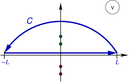
Figure 3: Integration contour $C$ for the verification of the Kubo formula (3.13). The poles $\nu_{+,\pm}$ ($\nu_{-,\pm}$) in the upper (lower) complex $\nu$-plane are indicated, for $|\omega|<\lambda/2$, by green filled (red open) circles. At the end, the limit $L\to\infty$ is taken.

$$R^{(s)}(\tau) \stackrel{{\scriptstyle?}}{{=}} \frac{2{\rm i}}{\hbar}\,\frac{1}{2\pi}\oint_{C}\!{\rm d}\nu\>{\rm e}^{{\rm i}\nu\tau}\frac{\hbar\lambda}{m}\frac{\nu}{(\nu^{2}+{\rm i}\lambda\nu-\omega^{2})}\frac{-1}{(\nu^{2}-{\rm i}\lambda\nu-\omega^{2})}$$ (3.15)

$$= \frac{2{\rm i}}{\hbar}\,\frac{1}{2\pi}\frac{\hbar\lambda}{m}\frac{1}{2{\rm i}\lambda}\oint_{C}\!{\rm d}\nu\>{\rm e}^{{\rm i}\nu\tau}\frac{-1}{(\nu^{2}-{\rm i}\lambda\nu-\omega^{2})}$$

$$= \frac{1}{\sqrt{2\pi\,}\,}\int_{\mathbb{R}}\!{\rm d}\nu\>{\rm e}^{{\rm i}\nu\tau}\frac{1}{m\sqrt{2\pi\,}\,}\frac{-1}{(\nu^{2}-{\rm i}\lambda\nu-\omega^{2})}$$

$$= \frac{1}{\sqrt{2\pi\,}\,}\int_{\mathbb{R}}\!{\rm d}\nu\>{\rm e}^{{\rm i}\nu\tau}\widehat{R}^{(s)}(\nu)$$

as required. Herein, in the first line the commutator $\widehat{C}_{-}^{(s)}(\nu)$ was inserted from (3.12); in the second line the residua at $\nu=\nu_{+,\pm}$ were computed according to (3.14) and finally the response function (3.10) was recognised. Of course, the contribution of the upper semi-arc is negligible.

This shows the validity of the Kubo formula (A.1,A.4) for the spin $s$. Its validity for the momentum $p$ is now obvious from (3.10) and (3.12).

Summarising: if for an ohmic dissipation, the only non-vanishing noise correlators are given by (3.9), then (i) for all times $t\geq 0$ the equal-time canonical commutator $\left\langle\left[s(t),p(t)\right]\right\rangle={\rm i}\hbar$ and (ii) for all time differences $\tau=t-t^{\prime}>0$ the Kubo formulæ for both the spin $s$ and the momentum $p$ hold true. This implements the criteria (A,B).

3.4 Anti-commutators and the virial theorem

It remains to analyse the admissible forms of the noise anti-correlators. Since the bath is stationary, we can start from

$$\left\langle\left\{\eta_{s}(t),\eta_{s}(t^{\prime})\right\}\right\rangle=2\beta(t-t^{\prime})\ ,\ \left\langle\left\{\eta_{p}(t),\eta_{p}(t^{\prime})\right\}\right\rangle=2\alpha(t-t^{\prime})\ ,\ \left\langle\left\{\eta_{s}(t),\eta_{p}(t^{\prime})\right\}\right\rangle=2\gamma(t-t^{\prime})$$ (3.16)

where the functions $\alpha(t)=\alpha(-t)$, $\beta(t)=\beta(-t)$ and $\gamma(t)$ must be found. In frequency-space this reads

$$\left\langle\left\{\widehat{\eta}_{s}(\nu),\widehat{\eta}_{s}(\nu^{\prime})\right\}\right\rangle = \delta(\nu+\nu^{\prime})\sqrt{2\pi\,}\>2\widehat{\beta}(\nu)$$

$$\left\langle\left\{\widehat{\eta}_{p}(\nu),\widehat{\eta}_{p}(\nu^{\prime})\right\}\right\rangle = \delta(\nu+\nu^{\prime})\sqrt{2\pi\,}\>2\widehat{\alpha}(\nu)$$ (3.17)

$$\left\langle\left\{\widehat{\eta}_{s}(\nu),\widehat{\eta}_{p}(\nu^{\prime})\right\}\right\rangle = \delta(\nu+\nu^{\prime})\sqrt{2\pi\,}\>2\widehat{\gamma}(\nu)$$

While $\widehat{\alpha}(\nu)$ and $\widehat{\beta}(\nu)$ are symmetric, there is no obvious symmetry for $\widehat{\gamma}(\nu)$. With the definition

$$C_{+}^{(s)}(\nu,\nu^{\prime}) =\frac{1}{2}\left\langle\left\{\widehat{s}(\nu),\widehat{s}(\nu^{\prime})\right\}\right\rangle=\delta(\nu+\nu^{\prime})\widehat{C}_{+}^{(s)}(\nu)$$ (3.18a)

$$C_{+}^{(p)}(\nu,\nu^{\prime}) =\frac{1}{2}\left\langle\left\{\widehat{p}(\nu),\widehat{p}(\nu^{\prime})\right\}\right\rangle=\delta(\nu+\nu^{\prime})\widehat{C}_{+}^{(p)}(\nu)$$ (3.18b)

we have from (3.3)

$$\widehat{C}_{+}^{(s)}(\nu) :=\frac{\frac{\widehat{\alpha}(\nu)}{m^{2}}+(\lambda^{2}+\nu^{2})\widehat{\beta}(\nu)+\frac{\lambda}{m}\left(\widehat{\gamma}(\nu)+\widehat{\gamma}(-\nu)\right)+\frac{{\rm i}\nu}{m}\left(\widehat{\gamma}(\nu)-\widehat{\gamma}(-\nu)\right)}{(\nu^{2}-{\rm i}\lambda\nu-\omega^{2})(\nu^{2}+{\rm i}\lambda\nu-\omega^{2})}$$ (3.19a)

$$\widehat{C}_{+}^{(p)}(\nu) :=\frac{\nu^{2}\widehat{\alpha}(\nu)+m^{2}\omega^{4}\widehat{\beta}(\nu)+{\rm i}m\omega^{2}\nu\left(\widehat{\gamma}(\nu)-\widehat{\gamma}(-\nu)\right)}{(\nu^{2}-{\rm i}\lambda\nu-\omega^{2})(\nu^{2}+{\rm i}\lambda\nu-\omega^{2})}$$ (3.19b)

The virial theorem states that $\widehat{C}_{+}^{(p)}(\nu)\stackrel{{\scriptstyle!}}{{=}}m^{2}\omega^{2}\widehat{C}_{+}^{(s)}(\nu)$, see appendix A. Combination with (3.19) leads to the condition

$$(\nu^{2}-\omega^{2})\widehat{\alpha}(\nu)+(m^{2}\omega^{4}-m^{2}\omega^{2}(\lambda^{2}+\nu^{2}))\widehat{\beta}(\nu)\stackrel{{\scriptstyle!}}{{=}}\lambda m\omega^{2}\left(\widehat{\gamma}(\nu)+\widehat{\gamma}(-\nu)\right)$$ (3.20)

The simplest solution is

$$\widehat{\alpha}(\nu)=\widehat{\beta}(\nu)=0\;\;,\;\;\widehat{\gamma}(\nu)+\widehat{\gamma}(-\nu)=0$$ (3.21)

It is the only solution which does not depend on the model’s parameters $m,\omega$. Any other solution must contain at least one of them. Since we are looking for a characterisation of the noises $\eta_{s},\eta_{p}$ which should be independent of the specific physical model under study, we shall retain the solution (3.21) as our implementation of the condition (C).

Inserting (3.21), the correlators take the form

$$\widehat{C}_{+}^{(s)}(\nu)=\frac{2{\rm i}}{m}\frac{\nu\widehat{\gamma}(\nu)}{(\nu^{2}-{\rm i}\lambda\nu-\omega^{2})(\nu^{2}+{\rm i}\lambda\nu-\omega^{2})}=\frac{1}{m^{2}\omega^{2}}\,\widehat{C}_{+}^{(p)}(\nu)$$ (3.22)

3.5 Quantum fluctuation-dissipation theorem

The form of the remaining antisymmetric function $\widehat{\gamma}(\nu)=-\widehat{\gamma}(-\nu)$ is found from the qfdt. As shown in appendix A, in frequency-space it can be written in the form

$$\frac{\widehat{C}_{+}^{(s)}(\nu)}{\widehat{C}_{-}^{(s)}(\nu)}=\frac{\widehat{C}_{+}^{(p)}(\nu)}{\widehat{C}_{-}^{(p)}(\nu)}=-\frac{1}{\sqrt{2\pi\,}\,}\coth\frac{\hbar\nu}{2T}$$ (3.23)

Therefore, comparison of (3.12) with (3.22) leads to the condition

$$2{\rm i}\sqrt{2\pi\,}\,\widehat{\gamma}(\nu)=\hbar\lambda\coth\frac{\hbar\nu}{2T}$$ (3.24)

which also implements the condition (D). This means that the only non-vanishing commutators and anti-commutators of the noises are

$$\left\langle\left\{\widehat{\eta}_{s}(\nu),\widehat{\eta}_{p}(\nu^{\prime})\right\}\right\rangle=\frac{\hbar\lambda}{{\rm i}}\coth\left(\frac{\hbar\nu}{2T}\right)\,\delta(\nu+\nu^{\prime})\;\;,\;\;\left\langle\left[\widehat{\eta}_{s}(\nu),\widehat{\eta}_{p}(\nu^{\prime})\right]\right\rangle={\rm i}\hbar\lambda\,\delta(\nu+\nu^{\prime})$$ (3.25)

They do depend on the assumption of ohmic dissipation and on the properties of the bath (here the temperature $T$). But since they do not contain the specific parameters $m,\omega$ of the harmonic oscillator model we used to derive them, they should be applicable in general.

It is possible to combine the equations of motion (1.2) into a single second-order Langevin equation, which reads [25, 26, 27]

$$\partial_{t}^{2}s+\lambda\partial_{t}s+\omega^{2}s=\zeta\;\;,\;\;\zeta=\frac{1}{m}\eta_{p}+\lambda\eta_{s}+\partial_{t}\eta_{s}$$ (3.26)

The second moments of the ‘composite noise’ $\zeta(t)$ are readily found, first in frequency space

$$\big{<}\big{\{}\widehat{\zeta}(\nu),\widehat{\zeta}(\nu^{\prime})\big{\}}\big{>}=\frac{2\hbar\lambda}{m}\,\nu\coth\left(\frac{\hbar\nu}{2T}\right)\>\delta(\nu+\nu^{\prime})\;\;,\;\;\big{<}\big{[}\widehat{\zeta}(\nu),\widehat{\zeta}(\nu^{\prime})\big{]}\big{>} =-\frac{2\hbar\lambda}{m}\>\nu\,\delta(\nu+\nu^{\prime})$$ (3.27)

and then for the times

$$\left\langle\left\{\zeta(t),\zeta(t^{\prime})\right\}\right\rangle =\frac{2\hbar\lambda}{\pi m}\int_{0}^{\infty}\!{\rm d}\nu\>\nu\coth\left(\frac{\hbar\nu}{2T}\right)\cos(\nu(t-t^{\prime}))\>=:\>\frac{\hbar\lambda}{\pi m}\,I\left(\frac{\hbar}{2T},t-t^{\prime}\right)$$ (3.28a)

$$\left\langle\left[\zeta(t),\zeta(t^{\prime})\right]\right\rangle =\frac{2\hbar\lambda}{{\rm i}\pi m}\int_{0}^{\infty}\!{\rm d}\nu\>\nu\sin(\nu(t-t^{\prime}))\hskip 59.75095pt\>=\>\>\frac{2{\rm i}\hbar\lambda}{m}\>\delta^{\prime}\left(t-t^{\prime}\right)$$ (3.28b)

which is the noise-averaged form of the ones proposed by Ford et al. [27, eqs. (2.2,2.3)]. Since the ‘composite noise’ $\zeta$ contains derivatives, it should be rougher than the individual noises $\eta_{s},\eta_{p}$. This feature might be useful for the construction of numerical approximation schemes for the qles (1.2).

Finally, converting (3.25) to real times leads to (as shown in appendix B)

$$\left\langle\bigl{\{}\eta_{s}(t),{\eta}_{p}(t^{\prime})\bigr{\}}\right\rangle=\lambda T\coth\left(\frac{\pi T}{\hbar}(t-t^{\prime})\right)\;\;,\;\;\left\langle\bigl{[}{\eta}_{s}(t),{\eta}_{p}(t^{\prime})\bigr{]}\right\rangle={\rm i}\hbar\lambda\,\delta(t-t^{\prime})$$ (3.29)

These are equivalent to the averages given in (1.6). Hence, the qfdt implies non-markovian noise correlators.

Our discussion of the stationary state has produced the necessary ingredients to undertake the study of the relaxation behaviour, starting from an arbitrary initial state. For the specific example of the qho, it is enough to take up the formal solution (2.7) and to use the quantum noise correlators (1.6). While the responses are (of course !) unchanged with respect to the treatment of section 2, the correlators will now obey the qfdt, by construction. The explicit results have been known since a long time, see [25, 26, 27, 31, 71] and references therein, we shall not repeat the explicit calculation.

Summarising: if the only non-vanishing second moments of the noises $\eta_{s},\eta_{p}$ are given by (3.29) (or equivalently by (3.25)), then the four criteria (A,B,C,D) for a quantum dynamics of the harmonic oscillator (1.2) are satisfied.

4 An example: the quantum spherical model

The classical spherical model was initially formulated as an exactly solvable variant of the Ising model, in $d$ spatial dimensions [6, 44]. For short-ranged interactions, and dimensions $2<d<4$, its second-order phase transition is in an universality class distinct from mean-field theory. The quantum spherical model is defined by the hamiltonian [51, 40, 66, 52, 67]

$$H=\sum_{\boldsymbol{n}\in\mathscr{L}}\left(-J\sum_{j=1}^{d}S_{\boldsymbol{n}}S_{\boldsymbol{n}+\boldsymbol{e}_{j}}+\frac{\mu}{2}S_{\boldsymbol{n}}^{2}+\frac{g}{2}P_{\boldsymbol{n}}^{2}\right)\;\;,\;\;\left[S_{\boldsymbol{n}},P_{\boldsymbol{m}}\right]={\rm i}\hbar\,\delta_{\boldsymbol{n},\boldsymbol{m}}$$ (4.1)

where $S_{\boldsymbol{n}}$ is the spin operator at the site $\boldsymbol{n}\in\mathscr{L}\subset\mathbb{Z}^{d}$ of a hyper-cubic lattice $\mathscr{L}$ with $|\mathscr{L}|=\cal N$ sites, $P_{\boldsymbol{n}}$ is the canonically conjugate momentum, the constants $J$ and $g$ describe the nearest-neighbour interactions and the kinetic energy, respectively, and $\mu$ is the Lagrange multiplier whose value is fixed by the (mean) spherical constraint $\left\langle\sum_{\boldsymbol{n}}S_{\boldsymbol{n}}^{2}\right\rangle={\cal N}$. In momentum space, the equations of motion of the different modes decouple, such that the quantum Langevin equations are

$$\partial_{t}\widehat{S}(t,\boldsymbol{q}) = g\widehat{P}(t,\boldsymbol{q})+\widehat{\eta}_{s}(t,\boldsymbol{q})$$

$$\partial_{t}\widehat{P}(t,\boldsymbol{q}) = -\frac{1}{g}\left(\mathfrak{z}(t)+\omega(\boldsymbol{q})\right)\widehat{S}(t,\boldsymbol{q})-\lambda\widehat{P}(t,\boldsymbol{q})+\widehat{\eta}_{p}(t,\boldsymbol{q})$$ (4.2)

with $\omega(\boldsymbol{q})=2\sum_{j=1}^{d}(1-\cos q_{j})$ and $\mu(t)=d+\mathfrak{z}(t)$. The spherical constraint, which in momentum space becomes $(2\pi)^{-d}\int_{\cal B}{\rm d}\boldsymbol{q}\>\left\langle\widehat{S}(t,\boldsymbol{q})\widehat{S}(t,-\boldsymbol{q})\right\rangle=1$, maintains a coupling between the modes and fixes $\mathfrak{z}(t)$ self-consistently (${\cal B}=[-\pi,\pi]^{d}$ is the Brillouin zone). Each mode relaxes separately to its equilibrium state whose (semi-)classical or quantum nature is determined by the noises.

Since the Lagrange multiplier $\mathfrak{z}(t)$ is time-dependent, this linear system cannot be solved via a straightforward matrix exponentiation (the time-dependent coefficient matrices do not commute for different times). Rather, the quite technical Magnus expansion [46, 9] must be considered. However, the long-time behaviour follows from a single first-order Langevin equation, which we shall now derive via a long-time scaling limit on the Langevin equations (4.2) and the associated noises. Considering this over-damped Langevin equations considerably simplifies the explicit solutions of the dynamics, to be presented in future work.

1. First, we consider the Bedeaux-Mazur noise correlators (1.3), enhanced by spatial locality. In momentum space, the noise correlators read

$$\left\langle\widehat{\eta}_{p}(t,\boldsymbol{q})\widehat{\eta}_{p}(t^{\prime},\boldsymbol{q}^{\prime})\right\rangle \!\!= \!\!\frac{\lambda\hbar\sqrt{\mathfrak{z}(t)+\omega(\boldsymbol{q})}}{g}\coth\left(\frac{\hbar\sqrt{\mathfrak{z}(t)+\omega(\boldsymbol{q})}}{2T}\right)\delta(t-t^{\prime})\delta(\boldsymbol{q}+\boldsymbol{q}^{\prime})$$

$$\left\langle\widehat{\eta}_{s}(t,\boldsymbol{q})\widehat{\eta}_{p}(t^{\prime},\boldsymbol{q}^{\prime})\right\rangle \!\!= \!\!-\left\langle\widehat{\eta}_{p}(t,\boldsymbol{q})\widehat{\eta}_{s}(t^{\prime},\boldsymbol{q}^{\prime})\right\rangle\>=\>\frac{1}{2}{\rm i}\hbar\lambda\,\delta(t-t^{\prime})\delta(\boldsymbol{q}+\boldsymbol{q}^{\prime})$$ (4.3)

Information on the long-time behaviour can be obtained by making the scaling transformation

$$\tau:=gt\;\;,\;\;\widehat{\eta}_{s}(t,\boldsymbol{q})=g^{3/2}\widetilde{\eta}_{s}(\tau,\boldsymbol{q})\;\;,\;\;\widehat{\eta}_{p}(t,\boldsymbol{q})=g^{-1/2}\widetilde{\eta}_{p}(\tau,\boldsymbol{q})\;\;,\;\;\widehat{S}(t,\boldsymbol{q})=g^{1/2}\widetilde{S}(\tau,\boldsymbol{q})$$ (4.4)

and then by considering the long-time scaling limit $g\to 0$, $t\to\infty$ such that $\tau=gt$ is kept fixed. Combining eqs. (4.2,4.3) leads to the equation of motion for the rescaled spin $\widetilde{S}(\tau,\boldsymbol{q})$

$$\underbrace{g^{2}\partial_{\tau}^{2}\widetilde{S}(\tau,\boldsymbol{q})-g^{2}\partial_{\tau}\widetilde{\eta}_{s}(\tau,\boldsymbol{q})}_{\mbox{\rm O($g^{2}$) $\to 0$}}=-\left(\mathfrak{z}(\tau)+\omega(\boldsymbol{q})\right)\widetilde{S}(\tau,\boldsymbol{q})-\lambda g\partial_{\tau}\widetilde{S}(\tau,\boldsymbol{q})+\widetilde{\eta}(\tau,\boldsymbol{q})$$ (4.5)

with the new effective noise $\widetilde{\eta}(\tau,\boldsymbol{q}):=\sigma\widetilde{\eta}_{s}(\tau,\boldsymbol{q})+g\widetilde{\eta}_{p}(\tau,\boldsymbol{q})$ and we also substituted $\mathfrak{z}(t)\mapsto\mathfrak{z}(\tau)$. The left-hand side of (4.5) vanishes in the scaling limit such that a classical over-damped equation of motion remains. In the over-damped case under consideration, $\lambda$ must be considered large, so that we actually let $\lambda\to\infty$, but such that $\sigma:=\lambda g$ is being kept fixed. Then the scaling limit (4.4) is well-defined. We have the final semi-classical Langevin equation

$$\sigma\partial_{\tau}\widetilde{S}(\tau,\boldsymbol{q})+\bigl{(}\mathfrak{z}(\tau)+\omega(\boldsymbol{q})\bigr{)}\widetilde{S}(\tau,\boldsymbol{q})=\widetilde{\eta}(\tau,\boldsymbol{q})$$ (4.6a)

$$\left\langle\widetilde{\eta}(\tau,\boldsymbol{q})\widetilde{\eta}(\tau^{\prime},\boldsymbol{q}^{\prime})\right\rangle=\sigma\hbar\sqrt{\mathfrak{z}(\tau)+\omega(\boldsymbol{q})\,}\,\coth\left(\frac{\hbar\sqrt{\mathfrak{z}(\tau)+\omega(\boldsymbol{q})}}{2T}\right)\delta(\tau-\tau^{\prime})\delta(\boldsymbol{q}+\boldsymbol{q}^{\prime})$$ (4.6b)

along with $\left\langle\bigl{[}\widetilde{\eta}(\tau,q),\widetilde{\eta}(\tau^{\prime},q^{\prime})\bigr{]}\right\rangle=0$. In eq. (4.6), two limit cases can be recognised:

1. $T\to\infty$. Eq. (4.6b) reduces to white noise $\left\langle\widehat{\eta}(\tau,\boldsymbol{q})\widehat{\eta}(\tau^{\prime},\boldsymbol{q}^{\prime})\right\rangle=2T\sigma\delta(\tau-\tau^{\prime})\delta(\boldsymbol{q}+\boldsymbol{q}^{\prime})$ and eq. (4.6a) describes the relaxation towards classical thermal equilibrium. Unsurprisingly, for sufficiently large temperatures, one is back to an effectively classical system.

   This appears analogous to the semi-classical behaviour of the quantum spherical model with Lindblad dynamics [69].

2. $T\to 0$. Then the noise correlator (4.6b) reduces to

   $$\left\langle\widehat{\eta}(\tau,\boldsymbol{q})\widehat{\eta}(\tau^{\prime},\boldsymbol{q}^{\prime})\right\rangle=\sigma\hbar\sqrt{\mathfrak{z}(\tau)+\omega(\boldsymbol{q})\,}\,\delta(\tau-\tau^{\prime})\delta(\boldsymbol{q}+\boldsymbol{q}^{\prime})$$ (4.7)

   Therefore, at vanishing temperature, the model shows some new type of non-classical behaviour, but which comes from a markovian dynamics. Further details will be presented elsewhere.

2. We now present the same analysis for the quantum noises (1.6) derived in section 3. The only non-vanishing noise anti-commutators and commutators are

$$\left\langle\bigl{\{}\widehat{\eta}_{s}(t,\boldsymbol{q}),\widehat{\eta}_{p}(t^{\prime},\boldsymbol{q}^{\prime})\bigr{\}}\right\rangle=\frac{\hbar\lambda}{2\pi}J\left(\frac{\hbar}{2T},t-t^{\prime}\right)\delta(\boldsymbol{q}+\boldsymbol{q}^{\prime})\;\;,\;\;\left\langle\bigl{[}\widehat{\eta}_{s}(t,\boldsymbol{q}),\widehat{\eta}_{p}(t^{\prime},\boldsymbol{q}^{\prime})\bigr{]}\right\rangle={\rm i}\hbar\lambda\delta(t-t^{\prime})\delta(\boldsymbol{q}+\boldsymbol{q}^{\prime})$$ (4.8)

where the function $J(a,\tau)$ is analysed in appendix B. We apply the scaling transformation

$$\tau:=gt\;\;,\;\;\widehat{\eta}_{s}(t,\boldsymbol{q})=g^{0}\widetilde{\eta}_{s}(\tau,\boldsymbol{q})\;\;,\;\;\widehat{\eta}_{p}(t,\boldsymbol{q})=g^{0}\widetilde{\eta}_{p}(\tau,\boldsymbol{q})\;\;,\;\;\widehat{S}(t,\boldsymbol{q})=g^{1}\widetilde{S}(\tau,\boldsymbol{q})$$ (4.9)

to eqs. (4.2), re-written in the form

$$\underbrace{g^{2}\partial_{\tau}\widetilde{S}(\tau,\boldsymbol{q})}_{\mbox{\rm O$(g^{2})\to 0$}}=-\bigl{(}\mathfrak{z}(\tau)+\omega(\boldsymbol{q})\bigr{)}\widetilde{S}(\tau,\boldsymbol{q})-\sigma\partial_{\tau}\widetilde{S}(\tau,\boldsymbol{q})+\widetilde{\zeta}(\tau,\boldsymbol{q})+\widetilde{\xi}(\tau,\boldsymbol{q})$$ (4.10)

with the two auxiliary noises

$$\widetilde{\zeta}(\tau,\boldsymbol{q}):=\widetilde{\eta}_{p}(\tau,\boldsymbol{q})+\sigma g^{-2}\widetilde{\eta}_{s}(\tau,\boldsymbol{q})\;\;,\;\;\widetilde{\xi}(\tau,\boldsymbol{q}):=\partial_{\tau}\widetilde{\eta}_{s}(\tau,\boldsymbol{q})$$ (4.11)

and consider the scaling limit $t\to\infty$, $g\to 0$ such that $\tau=gt$ is kept fixed. Herein, the rescaled dissipation rate $\sigma$ and the rescaled temperature $\Theta$ are

$$\sigma=\lambda g\;\;,\;\;\Theta=Tg^{-1}$$ (4.12)

Then the noise commutator

$$\left\langle\bigl{[}\widetilde{\zeta}(\tau,\boldsymbol{q})+\widetilde{\xi}(\tau,\boldsymbol{q}),\widetilde{\zeta}(\tau^{\prime},\boldsymbol{q}^{\prime})+\widetilde{\xi}(\tau^{\prime},\boldsymbol{q}^{\prime})\bigr{\}}\right\rangle=2{\rm i}\hbar\sigma\delta^{\prime}(\tau-\tau^{\prime})\delta(\boldsymbol{q}+\boldsymbol{q}^{\prime})$$ (4.13)

reproduces (3.28b) and noise anti-commutator, with $I(a,\tau)=\partial_{\tau}J(a,\tau)$

$$\left\langle\bigl{\{}\widetilde{\zeta}(\tau,\boldsymbol{q})+\widetilde{\xi}(\tau,q),\widetilde{\zeta}(\tau^{\prime},\boldsymbol{q}^{\prime})+\widetilde{\xi}(\tau^{\prime},\boldsymbol{q}^{\prime})\bigr{\}}\right\rangle=\frac{\hbar\sigma}{\pi}I\left(\frac{\hbar}{2\Theta},\tau-\tau^{\prime}\right)\delta(\boldsymbol{q}+\boldsymbol{q}^{\prime})$$ (4.14)

reduces exactly to the form (3.28a), with the mass set to $m=1$ and up to spatial correlations. Therefore, instead of (4.6), the Langevin equations now become

$$\sigma\partial_{\tau}\widetilde{S}(\tau,\boldsymbol{q})+\bigl{(}\mathfrak{z}(\tau)+\omega(\boldsymbol{q})\bigr{)}\widetilde{S}(\tau,\boldsymbol{q}) =\widetilde{\eta}(\tau,\boldsymbol{q})$$ (4.15a)

$$\left\langle\bigl{\{}\widetilde{\eta}(\tau,\boldsymbol{q}),\widetilde{\eta}(\tau^{\prime},\boldsymbol{q}^{\prime})\bigr{\}}\right\rangle =\frac{\sigma\hbar}{\pi}I\left(\frac{\hbar}{2\Theta},\tau-\tau^{\prime}\right)\delta(\boldsymbol{q}+\boldsymbol{q}^{\prime})$$ (4.15b)

$$\left\langle\bigl{[}\widetilde{\eta}(\tau,\boldsymbol{q}),\widetilde{\eta}(\tau^{\prime},\boldsymbol{q}^{\prime})\bigr{]}\right\rangle =2{\rm i}\sigma\hbar\,\delta^{\prime}(\tau-\tau^{\prime})\delta(\boldsymbol{q}+\boldsymbol{q}^{\prime})$$ (4.15c)

Clearly, we have two limit cases, using the asymptotics of $I(a,\tau)$ from appendix B:

1. $\Theta\to\infty$. One is back to classical white noise.

2. $\Theta\to 0$. The eq. (4.15b) becomes a pure quantum noise, with memory

   $$\left\langle\bigl{\{}\widetilde{\eta}(\tau,\boldsymbol{q}),\widetilde{\eta}(\tau^{\prime},\boldsymbol{q}^{\prime})\bigr{\}}\right\rangle=-\frac{2\sigma\hbar}{\pi}\left(\frac{1}{\tau-\tau^{\prime}}\right)^{2}\delta(\boldsymbol{q}+\boldsymbol{q}^{\prime})$$ (4.16)

   and eq. (4.15c) is kept.

	Bedeaux & Mazur	quantum
dissipation $\lambda$	increases for $g\to 0$	increases for $g\to 0$
temperature $T$	constant	decreases for $g\to 0$
line $T=0$	neutral	unstable
noises $\eta(t),\eta(t^{\prime})$	commute for $t\neq t^{\prime}$	do not commute

Table 1: Some physical characteristics of the scaling transformations (4.4,4.9), respectively, leading for $g\to 0$ to the overdamped Langevin equations (4.6a,4.15a), depending on the chosen dynamics.

In table 1, we collect some characteristics of the scaling transformation which lead to the overdamped Langevin equation (4.6a,4.15a), for either Bedeaux-Mazur noise (1.3) or else the quantum noise (1.6). The scaling limit generically leads to the overdamped limit $\lambda\to\infty$. In the quantum case, the zero-temperature line $T=0$ is unstable which means that the long-time behaviour for all $T>0$ should be the same as for the classical limit $T\to\infty$, while for Bedeaux-Mazur noise $T$ is not rescaled. Another important distinction concerns whether the noise commutator $\left\langle\bigl{[}\eta(t),\eta(t^{\prime})\bigr{]}\right\rangle$ vanishes for different times $t,t^{\prime}$ or not.

3. Finally, we illustrate some aspects of the non-markovian noise correlator (3.29). Consider a single qho, described by the qle (1.2), but with the noises (1.6). Following the lines of the treatment of section 2, the equal-time spin-spin correlator $C_{+}^{(s)}(t):=C_{+}^{(s)}(t,t)$ now becomes

$$C_{+}^{(s)}(t)=\frac{T}{2m}\int_{0}^{t}\!{\rm d}\tau\int_{0}^{t}\!{\rm d}\tau^{\prime}\>\coth\left(\frac{\pi T}{\hbar}(\tau-\tau^{\prime})\right)\left[{\rm e}^{-\Lambda_{+}(t-\tau)-\Lambda_{-}(t-\tau^{\prime})}-{\rm e}^{-\Lambda_{-}(t-\tau)-\Lambda_{+}(t-\tau^{\prime})}\right]$$ (4.17)

where $\Lambda_{\pm}$ are given in (2.2). For notational simplicity, and analogously to section 2, the initial conditions were chosen such that the non-stationary terms vanish.

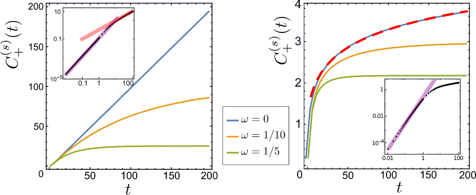
Figure 4: Time-dependence of the spin-spin correlator $C_{+}^{(s)}(t)$ (4.17) of the qho, for $m=\lambda=1$ and $\omega=[0,\frac{1}{10},\frac{1}{5}]$ from top to bottom.
(a) Left panel: $T=1$. At large times, the correlator saturates for $\omega>0$, while it diverges linearly for $\omega=0$. The inset shows, for $\omega=0$, the early-time behaviour $C_{+}^{(s)}\sim t^{2}$. The violet and red curves correspond to $\sim t^{2}$ and $\sim t$ behaviour, respectively and are guides to the eye.
(b) Right panel: $T=0$. The correlator saturates for $\omega\neq 0$ but grows logarithmically for $\omega=0$ (the red-dashed line is a guide to the eye). The inset shows again the short-time behaviour for $\omega=0$ and the violet curve $\sim t^{2}$ is a guide to the eye.

In figure 4, we illustrate the time-dependence of $C_{+}^{(s)}(t)$, for several values of $\omega$ and for two values of $T$ (units are such that $\hbar=1$).

1. The case $\omega>0$ corresponds to a harmonic coupling. In this case, for both $T=0$ and $T=1$, the correlator saturates rapidly, although the absolute scales are different. On the other hand, if one were to consider the qle (1.2) of the harmonic oscillator with a classical white noise instead, from (2.34) we would have found the constant $C_{+}^{(s)}=T/(m\omega^{2})$. The values of that constant indeed agree with the plateau values of the left panel in figure 4. Hence, for a finite temperature $T>0$, the effect of the quantum correlator (1.6) disappears after a finite cross-over time and for sufficiently large times, the system effectively behaves as if it were classical. For $T=0$, however, the values of the stationary correlator $C_{+}^{(s)}(\infty)$ are distinct from the classical values and the saturation occurs much faster.

2. The case $\omega=0$ can either be interpreted as a critical mode of a spin system or else as a diffusing quantum particle. In the latter case, $C_{+}^{(s)}(t)=\left\langle r^{2}(t)\right\rangle$ can be interpreted as the variance of the displacement of the quantum particle. Here, we find an important qualitative difference as a function of $T$. For $T=1$, the long-time variance $C_{+}^{(s)}(t)\sim t$ as for a classical particle (left panel), whereas for the case $T=0$ a logarithmic growth $C_{+}^{(s)}(t)\sim\ln t$ typical for quantum diffusion [36] is found (right panel).

   In the insets, for $\omega=0$ the early-time behaviour $C_{+}^{(s)}(t)\sim t^{2/z}$ is further illustrated. For both $T=0$ and $T=1$, an effectively ballistic behaviour with dynamical exponent $z=1$ is seen. This persists until the particles begin to encounter the obstacles created by the interactions with the bath. For $T=1$, one finds the cross-over to classical behaviour with $z=2$ while for $T=0$ one crosses over to quantum diffusion where $C_{+}^{(s)}(t)\sim\ln t$ grows logarithmically [36] and effectively $z=\infty$.

Turning now to the quantum spherical model, one has the qle eqs. (4.2), with the noise correlators (3.29) for each mode, but with an extra factor $\delta(\boldsymbol{q}+\boldsymbol{q}^{\prime})$. These modes are coupled by the spherical constraint, which in momentum space can be formally written as

$$\int_{\cal B}\frac{\!{\rm d}\boldsymbol{q}}{(2\pi)^{d}}\>\widehat{C}_{+}^{(s)}(t,t;\boldsymbol{q},-\boldsymbol{q})=1\ .$$ (4.18)

This makes the the spherical parameter $\mathfrak{z}=\mathfrak{z}(t)$ time-dependent. As a consequence, the matrix equation (4.2) cannot be solved by a formal matrix exponentiation. In principle, more elaborate tools such as a Magnus expansion or scaling ansätze should be tried but an explicit solution of (4.2) is still unknown. If such a solution could be found, solving eq. (4.18) would determine the Lagrange multiplier $\mathfrak{z}(t)$. Since the form of this equation is likely to be very different from the Volterra integral equations found for the classical spherical model [57, 33], its solution $\mathfrak{z}(t)$ should also be different from the classical result. We hope to return to this difficult open problem elsewhere.

Although the response functions do not depend explicitly on the noises, they do contain the Lagrange multiplier $\mathfrak{z}(t)$. Therefore, via the spherical constraint (4.18), the quantum noises will influence the long-time behaviour and the dynamical scaling of the two-time responses $R^{(s,p)}(t,t^{\prime})$.

5 Concludendum est

We presented attempts for an axiomatic construction of quantum Langevin equations. These have been based on four physical requirements which appeared reasonable to us, namely (A) canonical equal-time commutators, (B) the Kubo formulæ for spin and momentum, (C) the virial theorem and (D) the quantum fluctuation-dissipation theorem. The central role of the qfdt in this discussion stems not only from its recognised fundamental importance in quantum statistical mechanics [37, 71, 28] but also from its being an immediate consequence of an important dynamical symmetry for quantum equilibrium states [62, 2]. We used the harmonic oscillator equations of motion (1.2) as a scaffold to derive the second moments of the two noises $\eta_{s},\eta_{p}$. This form was motivated by the study of Bedeaux and Mazur [4, 5] although it turned out that their specific proposal (1.3), which is markovian, should be seen as a semi-classical description, since it only satisfies the criteria (A,B,C) while the condition (D) can only be satisfied in the classical limit $\hbar\to 0$. Furthermore, their noise correlators do depend on the specific model parameters $m,\omega$ of the harmonic oscillator and there is no obvious generalisation beyond this specific model. On the other hand, not requiring the Markov property from the outset does lead to a different approach where the noise correlators (1.6) (i) are model-independent and only contain bath properties (e.g. the temperature $T$) and the ohmic dissipation constant $\lambda$ (ii) are non-markovian as required from the validity of the quantum fluctuation-dissipation theorem for all $\hbar>0$. The noise correlators (1.6) are equivalent to the well-known second-order quantum Langevin equation of fkm, of a particle in an external potential [25, 27, 71]. It follows that the quantum noise correlators can indeed be derived from an Caldeira-Leggett-type independent oscillator model of the bath [25, 26, 27, 31, 71]. Still, the present re-derivation of a well-established result is of interest since the implicit assumptions behind each derivation are not entirely identical: while the derivation according to fkm [25, 26, 27] considers a particle in an arbitrary potential $V(s)$ and assumes explicitly a bath made from harmonic oscillators, our approach focusses on a single harmonic oscillator and proceeds to specify the second moments of the noise correlators, but does not assume neither gaussianity nor anything else specific about the bath. These two approaches produce the noise correlators (1.6,3.28) which are mathematically equivalent. It follows that the respective auxiliary assumptions are not really required. Hence the noise correlators (1.6) should be generally valid for the description of quantum dynamics, both for arbitrary potentials $V(s)$ as well as for a bath with non-harmonic degrees of freedom. In addition, the four properties (A,B,C,D) should be viewed as built-in features of Caldeira-Legget-type oscillator models of the bath. The present formalism also makes the symplectic structure more explicit.

On the other hand, different choices for the noise correlators are possible. Indeed, their generic form can be described in terms of two anti-symmetric functions $\chi(t)$ and $\psi(t)$ (see appendix C) and two symmetric functions $\alpha(t)$ and $\beta(t)$ (see section 3.4), but these functions do contain the specific model parameters $m,\omega$. All four criteria (A,B,C,D) are satisfied by these solutions but whose applicability is restricted to the harmonic oscillator. Eq. (1.6) is merely the only solution which does not depend on these parameters. Additional physical criteria, beyond considerations of maximal simplicity, are required to further specify these functions left undetermined and not contained in the Ford-Kac-Mazur construction [25, 26, 27].

We also used the quantum spherical model as an illustration how to set up the quantum equations of motion for an analysis of the long-time relaxational properties of this many-body problem. It turns out that such a constrained quantum dynamics leads to a formidable problem which has obtained a lot of attention, already since the early days of Dirac [19] and has been actively discussed recently, see e.g. [64, 68, 69, 35] and references therein. We presented a simple scaling argument which focusses on the long-time limit where an effective constrained Langevin equation should become more easily treatable. Work along these lines is in progress, with the aim of studying non-mean-field many-body quantum dynamics in higher spatial dimensions.

Acknowledgements: We are grateful to A. Chiocchetta, M. D. Coutinho-Filho, A. Gambassi, G.T. Landi, H. Spohn and L. Turban for useful discussions. SW thanks the LPCT Nancy for warm hospitality, where part of this work was carried out. RA acknowledges financial support from CAPES (Fundação do Ministério Brasileiro da Educação), process number 88881.132083/2016-01.

Appendix A.

We recall known results on three formulæ from quantum statistical mechanics. The notation will be adapted such as to be in agreement with the definition (3.1) of the Fourier transform.

A.1 Kubo formula

The Kubo formulæ are a generic result of linear-response theory, even outside a stationary state. For a quantum-mechanical system, its well-known time-dependent form is [15]

$$R(t-t^{\prime})=\frac{2{\rm i}}{\hbar}\,\Theta(t-t^{\prime})C_{-}(t,t^{\prime})=\frac{2{\rm i}}{\hbar}\,\Theta(t-t^{\prime})\frac{1}{2}\left\langle\left[s(t),s(t^{\prime})\right]\right\rangle$$ (A.1)

where for the sake of notational simplicity, we restrict attention to the response of a magnetic moment with respect to its canonically conjugated magnetic field.

In frequency-space, and for a stationary state, the commutator is written as follows

$$\frac{1}{2}\left\langle\left[\widehat{s}(\nu),\widehat{s}(\nu^{\prime})\right]\right\rangle=:\widehat{C}_{-}(\nu,\nu^{\prime})=:\delta(\nu+\nu^{\prime})\,\widehat{C}_{-}(\nu)$$ (A.2)

Using (3.1), the Kubo formula (A.1) becomes, if only $t-t^{\prime}>0$

$$\frac{1}{\sqrt{2\pi\,}\,}\int_{\mathbb{R}}\!{\rm d}\nu\>{\rm e}^{{\rm i}\nu(t-t^{\prime})}\widehat{R}(\nu) \stackrel{{\scriptstyle.}}{{=}} \frac{2{\rm i}}{\hbar}\frac{1}{2\pi}\int_{\mathbb{R}^{2}}\!{\rm d}\nu{\rm d}\nu^{\prime}\>{\rm e}^{{\rm i}\nu t+{\rm i}\nu^{\prime}t^{\prime}}\frac{1}{2}\left\langle\left[\widehat{s}(\nu),\widehat{s}(\nu^{\prime})\right]\right\rangle$$ (A.3)

$$= \frac{2{\rm i}}{\hbar}\frac{1}{2\pi}\int_{\mathbb{R}}\!{\rm d}\nu\>{\rm e}^{{\rm i}\nu t+{\rm i}\nu^{\prime}t^{\prime}}\delta(\nu+\nu^{\prime})\widehat{C}_{-}(\nu)$$

$$= \frac{2{\rm i}}{\hbar}\frac{1}{2\pi}\int_{\mathbb{R}}\!{\rm d}\nu\>{\rm e}^{{\rm i}\nu(t-t^{\prime})}\widehat{C}_{-}(\nu)$$

where (A.2) was used in the second line. Since this holds for all $t-t^{\prime}>0$, we have the relation between the amplitudes

$$\widehat{R}(\nu)\stackrel{{\scriptstyle.}}{{=}}-\frac{2}{\hbar{\rm i}}\frac{1}{\sqrt{2\pi\,}\,}\>\widehat{C}_{-}(\nu)$$ (A.4)

which we shall need below in the derivation of the qfdt. Momentum responses are treated analogously.

A.2 Virial theorem

The virial theorem is a well-known result of equilibrium statistical mechanics, with many important applications [38, 60]. A first quantum-mechanical derivation was given by Fock [24]. Consider a system of $N$ interacting particles with masses $m_{n}$, and with the hamiltonian

$$H=\sum_{n}\left(\frac{p_{n}^{2}}{2m_{n}}+V(\{x_{n}\})\right)$$ (A.5)

Use the momentum operator $p_{n}=\frac{\hbar}{{\rm i}}\frac{{\rm d}}{{\rm d}x_{n}}$ and define $\mathscr{V}:=\sum_{n}x_{n}p_{n}$. This gives

$$\frac{{\rm d}\mathscr{V}}{{\rm d}t}=\frac{{\rm i}}{\hbar}\left[H,\mathscr{V}\right]=2T-\sum_{n}x_{n}\frac{{\rm d}V}{{\rm d}x_{n}}$$ (A.6)

where $T=\frac{1}{2}\sum_{n}p_{n}^{2}/m_{n}$ denotes the kinetic energy. In a stationary state, with the quantum-mechanical average $\langle\cdot\rangle$, one has $\left\langle\frac{{\rm d}\mathscr{V}}{{\rm d}t}\right\rangle=0$, hence $2\left\langle T\right\rangle=\left\langle\sum_{n}x_{n}\frac{{\rm d}V}{{\rm d}x_{n}}\right\rangle$. Furthermore, if the potential is harmonic of degree $\alpha$ in all its arguments, that is $V(\lambda x_{n})=\lambda^{\alpha}V(x_{n})$ with $\lambda>0$ and for all $x_{n}$ with $n=1,\ldots,N$, this implies the virial theorem

$$\left\langle T\right\rangle=\frac{\alpha}{2}\left\langle V\right\rangle$$ (A.7)

Such stationary averages exist for $\alpha>-2$. For the harmonic oscillator, $\alpha=2$, hence $\left\langle T\right\rangle=\left\langle V\right\rangle$. If the system is a single harmonic oscillator, with $H=\frac{p^{2}}{2m}+\frac{m\omega^{2}}{2}x^{2}$, eq. (A.7) becomes $\left\langle p^{2}\right\rangle=m^{2}\omega^{2}\left\langle x^{2}\right\rangle$, or alternatively $C_{+}^{(p)}(t,t)=m^{2}\omega^{2}C_{+}^{(s)}(t,t)$ as quoted in the main text.

For extensions to relativistic quantum mechanics, see [24].

A.3 Kubo-Martin-Schwinger relation and the qfdt

Following [15], we recall the derivation of the Kubo-Martin-Schwinger (kms) relation for two-time quantities and use it to obtain the quantum fluctuation-dissipation theorem (qfdt).

At equilibrium, quantum correlators between the time-dependent observables $A,B$ are defined as

$$C_{AB}(t,t^{\prime})=\langle A(t)B(t^{\prime})\rangle:=\frac{1}{Z}\operatorname{tr}\left(A(t)B(t^{\prime})\rho(0)\right)$$ (A.8)

where $\rho(0)=\exp\left(-H/T\right)$ is the density matrix and $Z:=\operatorname{tr}\left(\rho(0)\right)$. In the Heisenberg representation, $A(t)=e^{{\rm i}/\hbar\,Ht}A(0)e^{-{\rm i}/\hbar\,Ht}$. Then the quantum correlator can be re-expressed as follows

$${C_{AB}(t,t^{\prime})=}\;\frac{1}{Z}\operatorname{tr}\left(B(t^{\prime})\>e^{-H/T}A(t)\right)$$ (A.9)

$$= \frac{1}{Z}\operatorname{tr}\left(B(t^{\prime})\>{\underbrace{{\color[rgb]{0,0,0}e^{-H/T}e^{{\rm i}/\hbar\,Ht}}}}\hskip 8.5359ptA(0)\hskip 48.36958pte^{-{\rm i}/\hbar\,Ht}\;\;\right)$$

$$= \frac{1}{Z}\operatorname{tr}\left(B(t^{\prime}){\color[rgb]{0,0,0}\underbrace{{\color[rgb]{0,0,0}\>e^{{\rm i}/\hbar\,H(t-\hbar/({\rm i}T))}A(0)\>}{\color[rgb]{1,1,1}e^{-{\rm i}/\hbar\,H(t-\hbar/({\rm i}T))}}}}{\overbrace{{\color[rgb]{0,0,0}e^{-{\rm i}/\hbar\,H(t-\hbar/({\rm i}T))}\>e^{{\rm i}/\hbar\,H(-\hbar/({\rm i}T))}}}}\>\right)$$

$$= \frac{1}{Z}\operatorname{tr}\left(B(t^{\prime})\hskip 45.52458ptA\left(t+\frac{{\rm i}\hbar}{T}\right)\hskip 71.13188pte^{-H/T}\;\right)$$

$${=} {C_{BA}\left(t^{\prime},t+\frac{{\rm i}\hbar}{T}\right)}$$

Symmetrising with respect to the times, the Kubo-Martin-Schwinger relation (A.9) becomes

$$C_{AB}(t-\frac{{\rm i}\hbar}{2T},t^{\prime})=C_{BA}(t^{\prime},t+\frac{{\rm i}\hbar}{2T})$$ (A.10)

In order to obtain the qfdt, we specialise to the case when $A=B$ and consider

$$C_{AA}(t,t^{\prime})=\frac{1}{2}\left\langle\left\{A(t),A(t^{\prime})\right\}\right\rangle+\frac{1}{2}\left\langle\left[A(t),A(t^{\prime})\right]\right\rangle=:C_{+}(t,t^{\prime})+C_{-}(t,t^{\prime})$$ (A.11)

Specifically, we shall take $A=s$ or $A=p$ in the text. Herein, $C_{+}(t,t^{\prime})=C_{+}(t^{\prime},t)$ is symmetric and $C_{-}(t,t^{\prime})=-C_{-}(t^{\prime},t)$ is antisymmetric. Then the kms relation (A.10) is

$$C_{+}\left(t^{\prime},t+\frac{{\rm i}\hbar}{2T}\right)+C_{-}\left(t^{\prime},t+\frac{{\rm i}\hbar}{2T}\right)=C_{+}\left(t-\frac{{\rm i}\hbar}{2T},t^{\prime}\right)+C_{-}\left(t-\frac{{\rm i}\hbar}{2T},t^{\prime}\right)$$ (A.12)

We use the symmetry and antisymmetry to recast this as

$$C_{+}\left(t+\frac{{\rm i}\hbar}{2T},t^{\prime}\right)-C_{+}\left(t-\frac{{\rm i}\hbar}{2T},t^{\prime}\right)=C_{-}\left(t+\frac{{\rm i}\hbar}{2T},t^{\prime}\right)+C_{-}\left(t-\frac{{\rm i}\hbar}{2T},t^{\prime}\right)$$

Next, use the Kubo formula (A.1) and the stationarity of $C_{+}=C_{+}(t-t^{\prime})$ and $R=R(t-t^{\prime})$ at equilibrium. This gives

$$C_{+}\left(t-t^{\prime}+\frac{{\rm i}\hbar}{2T}\right)-C_{+}\left(t-t^{\prime}-\frac{{\rm i}\hbar}{2T}\right)=-\frac{{\rm i}\hbar}{2}\left(R\left(t-t^{\prime}+\frac{{\rm i}\hbar}{2T}\right)+R\left(t-t^{\prime}-\frac{{\rm i}\hbar}{2T}\right)\right)$$

Fourier-transforming with respect to $\tau=t-t^{\prime}$, via (3.1), produces the qfdt

$$\tanh\left(\frac{\hbar\nu}{2T}\right)\widehat{C}_{+}(\nu)=\frac{{\rm i}\hbar}{2}\,\widehat{R}(\nu)$$ (A.13)

Finally, using the Kubo formula (A.4) brings the qfdt into the form

$$\frac{\widehat{C}_{+}(\nu)}{\widehat{C}_{-}(\nu)}=-\frac{1}{\sqrt{2\pi\,}\,}\coth\frac{\hbar\nu}{2T}$$ (A.14)

which is required in the text. Eq. (A.14) shows that $\widehat{C}_{+}^{(s)}/\widehat{C}_{-}^{(s)}=\widehat{C}_{+}^{(p)}/\widehat{C}_{-}^{(p)}$ is independent of the observable and only contains properties of the bath, as it should be.

Appendix B. Computation of an integral

We calculate the inverse Fourier transformation of (3.25) and derive (3.29). Then the subtle point of singular contributions to these inverse Fourier transforms is treated.

B.1 Regular functions

Consider

$$\left\langle\left\{\eta_{s}(t),\eta_{p}(t^{\prime})\right\}\right\rangle\>=\>\frac{1}{2\pi}\int_{\mathbb{R}^{2}}\!{\rm d}\nu{\rm d}\nu^{\prime}\>{\rm e}^{{\rm i}\nu t+{\rm i}\nu^{\prime}t^{\prime}}\left\langle\left\{\widehat{\eta}_{s}(\nu),\widehat{\eta}_{p}(\nu^{\prime})\right\}\right\rangle$$ (B.1)

$$= \frac{1}{2\pi}\int_{\mathbb{R}^{2}}\!{\rm d}\nu{\rm d}\nu^{\prime}\>{\rm e}^{{\rm i}\nu t+{\rm i}\nu^{\prime}t^{\prime}}\,\frac{\hbar\lambda}{{\rm i}}\coth\left(\frac{\hbar\nu}{2T}\right)\,\delta(\nu+\nu^{\prime})$$

$$= \frac{\hbar\lambda}{2\pi{\rm i}}\int_{\mathbb{R}}\!{\rm d}\nu\>{\rm e}^{{\rm i}\nu(t-t^{\prime})}\,\left[\coth\left(\frac{\hbar\nu}{2T}\right)-{\rm sign\,}\nu+{\rm sign\,}\nu\right]$$

$$= \frac{\hbar\lambda}{2\pi{\rm i}}\int_{\mathbb{R}}\!{\rm d}\nu\>{\rm e}^{{\rm i}\nu(t-t^{\prime})}\,{\rm sign\,}\nu+\frac{\hbar\lambda}{2\pi}\,2\int_{0}^{\infty}\!{\rm d}\nu\>\sin\left(\nu(t-t^{\prime})\right)\left[\coth\left(\frac{\hbar\nu}{2T}\right)-{\rm sign\,}\nu\right]$$

where (3.25) was used in the second line. In the last line, we separate into two contributions: (i) a singular integral which must be interpreted as a distribution and (ii) a regular convergent term, where the antisymmetry of the integrand was also used when retaining only the principal value of that second integral. This second term is given by the identity [55, eq. (2.5.46.17)]

$$\int_{0}^{\infty}\!{\rm d}x\>\sin(bx)\left[\coth(ax)-1\right]=\frac{\pi}{2a}\coth\left(\frac{\pi b}{2a}\right)-\frac{1}{b}$$ (B.2)

The first term in (B.1) is evaluated as a distribution [32, p. 173]: $\int_{\mathbb{R}}\!{\rm d}x\>{\rm e}^{{\rm i}\sigma x}\,{\rm sign\,}x=2{\rm i}\sigma^{-1}$. We then obtain

$$\left\langle\left\{\eta_{s}(t),\eta_{p}(t^{\prime})\right\}\right\rangle=\underbrace{\frac{\hbar\lambda}{\pi}\frac{1}{t-t^{\prime}}-\frac{\hbar\lambda}{\pi}\frac{1}{t-t^{\prime}}}_{=0}+\lambda T\coth\left(\frac{\pi T}{\hbar}(t-t^{\prime})\right)$$ (B.3)

which is (3.29) in the main text. We point out that the singular terms, arising in the intermediate states of the calculation, cancel in the final result.

Alternatively, the result (B.3) can be obtained from the identity [1, (4.3.91)]

$$\coth\frac{\hbar\nu}{2T}=\lim_{\varepsilon\to 0^{+}}\frac{2T\nu}{\hbar}\left(\frac{1}{(\nu+{\rm i}\varepsilon)(\nu-{\rm i}\varepsilon)}+2\sum_{n=1}^{\infty}\frac{1}{(\nu+{\rm i}\nu_{n})(\nu-{\rm i}\nu_{n})}\right)\;\;,\;\;\nu_{n}=\frac{2\pi T}{\hbar}\,n$$ (B.4)

Then, for $\tau>0$

$$\left\langle\left\{\eta_{s}(\tau),\eta_{p}(0)\right\}\right\rangle\>=\>\frac{\hbar\lambda}{2\pi{\rm i}}\int_{\mathbb{R}}\!{\rm d}\nu\>{\rm e}^{{\rm i}\nu\tau}\,\coth\left(\frac{\hbar\nu}{2T}\right)$$ (B.5)

$$= \frac{\lambda T}{{\rm i}\pi}\lim_{\varepsilon\to 0^{+}}\oint_{{\cal C}}\!{\rm d}\nu\>\left[\frac{\nu{\rm e}^{{\rm i}\nu\tau}}{(\nu+{\rm i}\varepsilon)(\nu-{\rm i}\varepsilon)}+\sum_{n=1}^{\infty}\frac{2\nu{\rm e}^{{\rm i}\nu\tau}}{(\nu+{\rm i}\nu_{n})(\nu-{\rm i}\nu_{n})}\right]$$

$$= \frac{\lambda T}{{\rm i}\pi}\,2\pi{\rm i}\lim_{\varepsilon\to 0^{+}}\left[\frac{{\rm i}\varepsilon{\rm e}^{-\varepsilon\tau}}{2{\rm i}\varepsilon}+\sum_{n=1}^{\infty}\frac{2{\rm i}\nu_{n}{\rm e}^{-\nu_{n}\tau}}{2{\rm i}\nu_{n}}\right]$$

$$= 2\lambda T\left[\frac{1}{2}+\sum_{n=1}^{\infty}\exp\left(-\frac{2\pi T\tau}{\hbar}n\right)\right]$$

$$= \lambda T\coth\left(\frac{\pi T}{\hbar}\tau\right)$$

where the integrals are re-expressed as contour integrals which are closed in the upper complex $\nu$-plane such that only the pôles with positive imaginary part will contribute. The last sum in the 4^th line is evaluated using the geometric series. Since the result is anti-symmetric in $\tau$ (as it should be), one can continue it to the domain $\tau<0$.

Comment: the above derivation implicitly assumes that both times are strictly real. If for reasons of causality, a small imaginary part is introduced, viz. $t-t^{\prime}\mapsto t-t^{\prime}+{\rm i}\varepsilon$, one has the identity $\frac{1}{\tau+{\rm i}\varepsilon}={\rm P}\frac{1}{\tau}-{\rm i}\pi\delta(\tau)$ [32], where ${\rm P}$ denotes the principal part, such that (B.3) would be replaced by

$$\left\langle\left\{\eta_{s}(t),\eta_{p}(t^{\prime})\right\}\right\rangle=\frac{\hbar\lambda}{\pi}\left(-{\rm i}\pi\delta(t-t^{\prime})\right)+\lambda T\coth\left(\frac{\pi T}{\hbar}(t-t^{\prime})\right)$$

and (1.6) would turn into

$$\left\langle\eta_{s}(t)\eta_{p}(t^{\prime})\right\rangle=\frac{\lambda T}{2}\coth\left(\frac{\pi T}{\hbar}(t-t^{\prime})\right)\;\;,\;\;\left\langle\eta_{p}(t)\eta_{s}(t^{\prime})\right\rangle=-{\rm i}\hbar\lambda\delta(t-t^{\prime})-\frac{\lambda T}{2}\coth\left(\frac{\pi T}{\hbar}(t-t^{\prime})\right)$$ (B.5)

B.2 Essential singularities and singular contributions

The presentation given in the above sub-section concentrates on the situations where all variables are finite. However, there are certain essential singularities, which must be described in terms of singular functions(i.e. distributions). Reconsider the average anti-commutator $\langle\{\eta_{s}(\tau),\eta_{p}(0)\}\rangle=\frac{\hbar\lambda}{2\pi}J\left(\frac{\hbar\lambda}{2T},\tau\right)$. The integral $J(a,\tau)$ is recast into a scaling from as follows, where $a\geq 0$ is admitted throughout.

$$J(a,\tau)\>:=\>\int_{\mathbb{R}}\!{\rm d}\nu\>\coth(a\nu)\>\frac{e^{{\rm i}\nu\tau}}{{\rm i}}\>=\>\int_{\mathbb{R}}\!{\rm d}\nu\>{\rm sign\,}\nu\,\frac{\coth a|\nu|}{\nu^{2}}\sin\nu\tau$$ (B.6)

$$= \int_{\mathbb{R}}\!{\rm d}\nu\>{\rm sign\,}\nu\left[\frac{\coth a|\nu|}{\nu^{2}}-1\right]\sin\nu\tau+\int_{\mathbb{R}}\!{\rm d}\nu\>{\rm sign\,}\nu\sin\nu\tau$$

$$= \int_{\mathbb{R}}\!{\rm d}\nu\>{\rm sign\,}\nu\>\frac{e^{-a|\nu|}}{\sinh a|\nu|}\sin\nu\tau+\frac{2}{\tau}$$

$$= \frac{2}{\tau}\left(1+\frac{\tau}{a}\int_{0}^{\infty}\!{\rm d}x\>\frac{e^{-x}}{\sinh x}\sin\left(x\frac{\tau}{a}\right)\right)\>=:\>\frac{1}{\tau}\mathscr{J}\left(\frac{\tau}{a}\right)$$

where in the third line, the singular integral was expressed as a distribution [32, p. 174]. The scaling function $\mathscr{J}(y)$ is well-defined for all finite values of $y$, but has an essential singularity at $y\to\infty$.

For the discussion of the physical properties in terms of the scaling variable $y=\tau/a$, we shall throughout fix $\tau$ and consider the limits $a\to 0$ and $a\to\infty$, respectively. First, for $a\to\infty$, one can straightforwardly expand in $1/a$, with the result, using [55, (2.4.10.14)] and [1, (23.1.3)]

$$J(a,\tau) \simeq \frac{2}{\tau}\left(1+\left(\frac{\tau}{a}\right)^{2}\int_{0}^{\infty}\!{\rm d}x\>\frac{x\,e^{-x}}{\sinh x}-\frac{1}{6}\left(\frac{\tau}{a}\right)^{4}\int_{0}^{\infty}\!{\rm d}x\>\frac{x\textthreesuperior\,e^{-x}}{\sinh x}+{\rm O}(a^{-6})\right)$$ (B.7)

$$= \frac{2}{\tau}\left(1+\frac{\pi^{2}}{12}\left(\frac{\tau}{a}\right)^{2}-\frac{\pi^{4}}{720}\left(\frac{\tau}{a}\right)^{4}+{\rm O}(a^{-6})\right)\hfill\mbox{\rm~{};~{}~{} $a\to\infty$}$$

Second, for $a\to 0$, rapid oscillations cause that the main contribution to the integral comes from around $x\approx 0$. Expanding $e^{-x}/\sinh x\simeq x^{-1}-1+\frac{1}{3}x+{\rm O}(x^{2})$, the leading behaviour is described in terms of distributions

$$J(a,\tau) \simeq \frac{2}{\tau}\left(1+\frac{1}{2}\frac{\tau}{a}\int_{\mathbb{R}}\!{\rm d}x\>\left[\frac{1}{|x|}-1+\frac{|x|}{3}+\ldots\right]{\rm sign\,}x\sin\left(x\frac{\tau}{a}\right)\right)$$ (B.8)

$$= \frac{\pi}{a}{\rm sign\,}\tau-\frac{2\pi}{3}a\delta^{\prime}(\tau)+{\rm O}(a^{2})\hfill\mbox{\rm~{};~{}~{} $a\to 0$}$$

where again [32, p. 174, eqs.(17,19,21)] was used (the prime indicates the derivative). We also see that the terms of order $1/\tau$, which arose in (B.6) as distributions, cancel. For the calculation of derivatives of $J(a,\tau)$, the property $\partial_{\tau}{\rm sign\,}\tau=2\delta(\tau)$ [32, p. 22] must be used.

Similarly, we consider the integral

$$I(a,\tau)\>:=\>\partial_{\tau}J(a,\tau)\>=\>\int_{\mathbb{R}}\!{\rm d}\nu\>\nu\,\coth(a\nu)\,e^{{\rm i}\nu\tau}$$ (B.11)

$$= \frac{2}{\tau^{2}}\left(-1+\left(\frac{\tau}{a}\right)\int_{0}^{\infty}\!{\rm d}x\>\frac{xe^{-x}}{\sinh x}\cos\left(x\frac{\tau}{a}\right)\right)\>=\>\frac{1}{\tau^{2}}\mathscr{I}\left(\frac{\tau}{a}\right)$$

$$\simeq \left\{\begin{array}[]{ll}\frac{2\pi}{a}\delta\left(\tau\right)-\frac{2\pi}{3}a\,\delta^{\prime\prime}\left(\tau\right)+\ldots&\mbox{\rm~{};~{}~{} $a\to 0$}\\[4.26773pt] \frac{2}{\tau^{2}}\left(-1+\frac{\pi^{2}}{12}\left(\frac{\tau}{a}\right)^{2}-\frac{\pi^{4}}{240}\left(\frac{\tau}{a}\right)^{4}+\ldots\right)&\mbox{\rm~{};~{}~{} $a\to\infty$}\end{array}\right.$$

which arises from the noise anticommutator $\left\langle\bigl{\{}\zeta(\tau),\zeta(0)\bigr{\}}\right\rangle=\frac{2\hbar\lambda}{\pi m}I\left(\frac{\hbar}{2T},\tau\right)$ of the qle (3.26). The asymptotic forms (B.11) can either be derived analogously as before or by direct differentiation from (B.7,B.8), together with the identity $\partial_{\tau}\left(|\tau|^{n}{\rm sign\,}\tau\right)=n|\tau|^{n-1}$, for $n\in\mathbb{Z}$ and $n\neq 0$ [32, p. 52, eq. (10)].

Appendix C. More details on noise commutators

We analyse generic noise commutators

$$\left\langle\big{[}\widehat{\eta}_{s}(\nu),\widehat{\eta}_{s}(\nu^{\prime})\big{]}\right\rangle=\delta(\nu+\nu^{\prime}){\rm i}\hbar\widehat{\psi}(\nu)\;\;,\;\;\left\langle\big{[}\widehat{\eta}_{p}(\nu),\widehat{\eta}_{p}(\nu^{\prime})\big{]}\right\rangle=\delta(\nu+\nu^{\prime}){\rm i}\hbar\widehat{\chi}(\nu)$$ (C.1)

along with $\left\langle\big{[}\widehat{\eta}_{s}(\nu),\widehat{\eta}_{p}(\nu^{\prime})\big{]}\right\rangle=\delta(\nu+\nu^{\prime}){\rm i}\hbar\widehat{\kappa}(\nu)$, instead of (3.4), where $\widehat{\psi}$, $\widehat{\chi}$ and $\widehat{\kappa}$ are unknown functions. With the definition (3.11), the spin-spin and momentum-momentum correlators read

$$\widehat{C}_{-}^{(s)}(\nu) =\frac{\delta(\nu+\nu^{\prime}){\rm i}\hbar\sqrt{\pi/2}}{(\omega^{2}-\nu^{2})^{2}+\lambda^{2}\nu^{2}}\bigg{(}\frac{1}{m^{2}}\widehat{\chi}(\nu)+(\lambda^{2}+\nu^{2})\widehat{\chi}(\nu)+\frac{{\rm i}\nu+\lambda}{m}\widehat{\kappa}(\nu)+\frac{{\rm i}\nu-\lambda}{m}\widehat{\kappa}(-\nu)\bigg{)}$$ (C.2)

$$\widehat{C}_{-}^{(p)}(\nu) =\frac{\delta(\nu+\nu^{\prime}){\rm i}\hbar\sqrt{\pi/2}}{(\omega^{2}-\nu^{2})^{2}+\lambda^{2}\nu^{2}}\bigg{(}\nu^{2}\widehat{\chi}(\nu)+m^{2}\omega^{4}\widehat{\psi}(\nu)+{\rm i}m\omega^{2}\nu(\widehat{\kappa}(\nu)+\widehat{\kappa}(-\nu))\bigg{)}$$ (C.3)

Since the choice of the average noise correlators does not affect the response functions (3.10), a necessary requirement of the validity of the Kubo formulæ, see (2.24), is that (3.12) holds true, viz. $\widehat{C}_{-}^{(p)}(\nu)\stackrel{{\scriptstyle!}}{{=}}{m^{2}\omega^{2}}\widehat{C}_{-}^{(s)}(\nu)$ (recall again (3.11)). This leads to the condition, for all $\nu>0$

$$\nu^{2}\widehat{\chi}(\nu)+m^{2}\omega^{4}\widehat{\psi}(\nu)+{\rm i}m\omega^{2}\nu\left(\widehat{\kappa}(\nu)+\widehat{\kappa}(-\nu)\right)$$ (C.4)

$$\stackrel{{\scriptstyle!}}{{=}} \omega^{2}\widehat{\chi}(\nu)+m^{2}\omega^{2}\left(\lambda^{2}+\nu^{2}\right)\widehat{\psi}(\nu)+m\omega^{2}\Bigl{(}{\rm i}\nu\left(\widehat{\kappa}(\nu)+\widehat{\kappa}(-\nu)\right)+\lambda\left(\widehat{\kappa}(\nu)-\widehat{\kappa}(-\nu)\right)\Bigr{)}~{}~{}~{}$$

The most simple solution is (which is independent of the model parameters $\omega,m$)

$$\widehat{\chi}(\nu)=\widehat{\psi}(\nu)=0\;\;,\;\;\widehat{\kappa}(\nu)-\widehat{\kappa}(-\nu)=0$$ (C.5)

Hence the form of the noise commutator correlations assumed in (3.4), with $\widehat{\kappa}(\nu)$ even, is the most simple formulation of a necessary condition for the validity of the Kubo formulæ. This further implies that the commutator $\left\langle\bigl{[}s(\tau),p(0)\bigr{]}\right\rangle$ is even in $\tau$, as illustrated in fig. 2.

References

• [1] M. Abramowitz and I.A. Stegun, Handbook of Mathematical Functions, Dover (New York 1965).
• [2] C. Aron, G. Biroli, L.F. Cugliandolo, Sci Post Phys. 4 008 (2018) [arxiv:1705.10800].
• [3] R. Becker, Theorie der Wärme, 2nd ed., Springer (Heidelberg 1978).
• [4] D. Bedeaux, P. Mazur, Mesoscopic non-equilibrium thermodynamics for quantum systems, Physica A298, 81 (2001).
• [5] D. Bedeaux, Non-equilibrium thermodynamics for quantum systems, Techn. Mechanik 22, 89 (2002).
• [6] T.H. Berlin, M. Kac, Spherical model of a ferromagnet, Phys. Rev. 86, 821 (1952).
• [7] R.F. Bienzobaz, S.R. Salinas, Quantum spherical model with competing interactions, Physica A391, 6399 (2012) [arxiv:1203.4073].
• [8] R.F. Bienzobaz, S.R. Salinas, Modelo esférico quântico elementar, Rev. Bras. Ens. Física 35, 3311 (2013).
• [9] S. Blanes, F. Casas, J.A. Oteo, J. Ros, The Magnus expansion and some of its applications, Phys. Rep. 470, 151 (2009) [arXiv:0810.5488].
• [10] H.-P. Breuer and F. Petruccione, The theory of open quantum systems, Oxford University Press (Oxford 2002).
• [11] H.J. Carmichael, Statistical methods in quantum optics 1, Springer (Heidelberg 1999).
• [12] J.R. Choi, Superposition states for quantum nanoelectronic circuits and their nonclassical properties, Int. Nano Lett. 7, 69 (2017).
• [13] A. Coniglio, P. Ruggiero, M. Zanetti, Scaling and crossover in the large-$N$ model for growth kinetics, Phys. Rev. E50, 1046 (1994) [arXiv:cond-mat/9405003].
• [14] A. Crépieux, Out-of-equilibrium fluctuation-dissipation relations verified by the electrical and thermoelectrical AC-conductances in a quantum dot, Ann. Physik 529, 1600344 (2017) [arxiv:1610.10011].
• [15] L.F. Cugliandolo, in J.-L. Barrat, M. Feiglman, J. Kurchan, J. Dalibard (eds), Slow relaxations and non-equilibrium dynamics in condensed matter, Les Houches LXXVII, Springer (Heidelberg 2003), pp. 367-521 [arxiv:cond-mat/0210312].
• [16] L.F. Cugliandolo, G.S. Lozano, N. Nessi, M. Picco, A. Tartaglia, Quenched dynamics of classical isolated systems: the spherical model with two-body random interactions or the Neuman integrable model, [arxiv:1712.07688].
• [17] T. Dauxois, S. Ruffo, E. Arrimondo, M. Wilkens (eds), Dynamics and thermodynamics of systems with long-range interactions: an introduction, Springer Lecture Notes in Physics 602, Springer (Heidelberg 2002).
• [18] L. Dinis, P. Martin, J. Barral, J. Prost, J.F. Joanny, Fluctuation-response theorem for the active noisy oscillator of the hair-cell bundle, Phys. Rev. Lett. 109, 160602 (2012) [arxiv:1409.6483].
• [19] P.A.M. Dirac, Generalized Hamiltonian dynamics, Proc. Roy. Soc. A246, 326 (1958).
• [20] X. Durang, M. Henkel, Exactly solvable models of growing interfaces and lattice gases: the Arcetri models, ageing and logarithmic sub-ageing, J. Stat. Mech. P123206 (2017) [arxiv:1708.08237].
• [21] M. Ebbinghaus, H. Grandclaude, M. Henkel, Absence of logarithmic scaling in the ageing behaviour of the $4D$ spherical model, Eur. Phys. J. B63, 85 (2008) [arXiv:0709.3220].
• [22] B.-G. Englert, G. Morigi, in A. Buchleitner and K. Hornberger (eds) Coherent Evolution in Noisy Environments, Springer Lecture Notes in Physics 611, Springer (Heidelberg 2002); pp. 55-106; [arxiv:quant-ph/0206116].
• [23] A. Erdelyi et al., Table of integral transforms, vol. 1, Mc Graw Hill (New York 1954).
• [24] V. Fock, Bemerkung zum Virialsatz, Z. Physik 63, 855 (1930).
• [25] G.W. Ford, M. Kac, P. Mazur, Statistical mechanics of assemblies of coupled oscillators, J. Math. Phys. 6, 504 (1965).
• [26] G.W. Ford, M. Kac, On the quantum Langevin equation, J. Stat. Phys. 46, 803 (1987).
• [27] G.W. Ford, J.T. Lewis, R.F. O’Connell, Quantum Langevin equation, Phys. Rev. A37, 4419 (1988).
• [28] G.W. Ford, The fluctuation-dissipation theorem, Contemporary Physics 58, 244 (2017).
• [29] N. Fusco, M. Zannetti, Relaxation and overlap-probability function in the spherical and mean-spherical models, Phys. Rev. E66, 066113 (2002) [cond-mat/0210502].
• [30] J. Gabelli, G. Fève, J.-M. Berroir, B. Plaçais, A coherent RC circuit, Rep. Prog. Phys. 75, 126504 (2012) [arxiv:1210.2874].
• [31] C. Gardiner and P. Zoller, Quantum Noise, Springer (Heidelberg 2004).
• [32] I.M. Gelfand, G.E. Shilov, Generalised functions, vol. 1, Academic Press (London 1964).
• [33] C. Godrèche, J.-M. Luck, Response of non-equilibrium systems at criticality: ferromagnetic models in dimension two and above, J. Phys. A: Math. Gen. 33, 9141 (2000) [arxiv:cond-mat/0001264].
• [34] I.S. Gradshteyn, I.M. Ryzhik, Table of integrals, series and products, 7th ed., Elsevier (Amsterdam 2007).
• [35] A.C.T. Gustavsson, Constrained quantum dynamics, Journal of Physics: Conf. Series 174, 012025 (2009), [arXiv:0903.5437].
• [36] V. Hakim, V. Ambegaokar, Quantum theory of a free particle interacting with a linearly dissipative environment, Phys. Rev. A32, 423 (1985).
• [37] P. Hänggi, G.-L. Ingold, Fundamental aspects of quantum Brownian motion, Chaos 15, 026105 (2005), [arXiv:quant-ph/0412052].
• [38] M. Harwitt, Astrophysical concepts, 4th ed., Springer (Heidelberg 2006).
• [39] M.O. Hase, S.R. Salinas, Dynamics of a mean spherical model with competing interactions, J. Phys. A: Math. Gen. 39, 4875, 2006 [arxiv:cond-mat/0512286].
• [40] M. Henkel, C. Hoeger, Hamiltonian formulation of the spherical model in $d=r+1$ dimensions, Z. Physik B55, 67 (1984).
• [41] J.F. Johnson, Hybrid infrared focal plane signal and noise model, IEEE Transactions Electron Devices 46, 96 (1999).
• [42] J.B. Kogut, An introduction to lattice gauge theory and spin systems, Rev. Mod. Phys. 51, 659 (1979).
• [43] K. Kubo, K. Asano, A. Shimizu, Macroscopic quantum violation of the fluctuation-dissipation theorem in equilibrium, Phys. Rev. B98, 115429 (2018) [arxiv:1804.03841].
• [44] H.W. Lewis, G.H. Wannier, Spherical model of a ferromagnet, Phys. Rev. 88, 682 (1952); erratum 90, 1131 (1953).
• [45] K.H. Lundberg, Noise sources in bulk CMOS, (preprint 2002), available at http://web.mit.edu/klund/www/papers/UNP_noise.pdf
• [46] W. Magnus, On the exponential solution of differential equations for a linear operator, Comm. Pure Appl. Math. 7, 649 (1954).
• [47] A. Maraga, A. Chiocchetta, A. Mitra, A. Gambassi, Ageing and coarsening in isolated quantum systems after a quench: exact results for the quantum ${\rm O}(N)$-model with $N\to\infty$, Phys. Rev. E92, 042151 (2015) [arXiv:1506.04528].
• [48] P. Martin, A.J. Hudspeth, F. Jülicher, Comparion of a hair-bundle’s spontaneous oscillations with its response to mechanical stimulation revels the underlying active process, PNAS 98, 14380 (2001).
• [49] H. Mo, F. van den Bosch, S. White, Galaxy formation and evolution, Cambridge Univ. Press (Cambridge 2010).
• [50] Th.M. Nieuwenhuizen, Quantum description of spherical spins, Phys. Rev. Lett. 74, 4293 (1995) [arxiv:cond-mat/9408056].
• [51] G. Obermair, in J.I. Budnick, M.P. Kawars (eds), Dynamical Aspects of Critical Phenomena, Gordon and Breach (New York 1972), p. 137.
• [52] M.H. Oliveira, E.P. Raposo, M.D. Coutinho-Filho, Quantum spherical spin model on hypercubic lattices, Phys. Rev. B74, 184101, 2006.
• [53] F. de Pasquale, P. Ruggiero, M. Zannetti, Noise spectrum in the quantum Langevin equation, J. Phys. A17, 1489 (1984).
• [54] A. Picone, M. Henkel, Response of non-equilibrium systems with long-range initial correlations, J. Phys. A35, 5575 (2002) [cond-mat/0203411].
• [55] A.P. Prudnikov, Yu.A. Brychkov, O.I. Marichev, Integrals and series, vol. 1: elementary functions, Gordon and Breach (New York 1986).
• [56] M. Rokni, P. Chandra, Dynamical study of the disordered quantum $p=2$ spherical model, Phys. Rev. B69, 094403 (2004) [arxiv:cond-mat/0301166].
• [57] G. Ronca, Dynamics of ferromagnets: Langevin approach to the mean spherical model, J. Chem. Phys. 68, 3737 (1978).
• [58] S. Sachdev, Quantum phase transitions, 2nd ed., Cambridge University Press (Cambridge 2011).
• [59] R. Sarpeshkar, T. Delbrück, C.A. Mead, White noise in MOS transistors and resistors, IEEE Circuits and Devices Magazine 9, 23 (1993).
• [60] P. Schneider, Extragalaktische Astronomie und Kosmologie, Springer (Heidelberg 2008).
• [61] B. Sciolla, G. Biroli, Quantum quenches, dynamical transitions and off-equilibrium quantum criticality, Phys. Rev. B88, 201110(R) (2013), [arxiv:1211.2572].
• [62] L.M. Sieberer, A. Chiocchetta, A. Gambassi, U.C. Täuber, S. Diehl, Thermodynamic equilibrium as a symmetry of the Schwinger-Keldysh action, Phys. Rev. B92, 134307 (2015) [arxiv:1505.00912].
• [63] U.C. Täuber, Critical dynamics: a field-theory approach to equilibrium and non-equilibrium scaling behaviour, Cambridge University Press (Cambridge 2014).
• [64] A.M. Timpanaro, S. Wald, F. Semião, G.T. Landi, Work-induced constrained quantum dynamics, [arXiv:1807.04374]
• [65] U. Vool, M. Devoret, Introduction to quantum electromagnetic circuits, Int. J. Circuit Theory Appl. 45, 897 (2017) [arxiv:1610.03438].
• [66] T. Vojta, Quantum version of a spherical model: Crossover from quantum to classical critical behaviour, Phys. Rev. B53, 710 (1996).
• [67] S. Wald, M. Henkel, Quantum phase transition in the spin-anisotropic quantum spherical model, J. Stat. Mech. P07006 (2015) [arXiv:1503.06713]
• [68] S. Wald, M. Henkel, Lindblad dynamics of a quantum spherical spin, J. Phys. A: Math. Theor. 49, 125001 (2016) [arxiv:1511.03347].
• [69] S. Wald, G.T. Landi, M. Henkel, Lindblad dynamics of the quantum spherical model, J. Stat. Mech. 013103 (2018) [arXiv:1707.06273].
• [70] S. Wald, M. Henkel, On integral representations and asymptotics of some hypergeometric functions in two variables, Int. Transforms Spec. Funct. 29, 95 (2018) [arxiv:1707.06275].
• [71] U. Weiss, Quantum dissipative systems, 4th ed., World Scientific (Singapour 2012).