On a gap between rational annuitization price for producer and price for customer

Abstract

The paper studies pricing of insurance products focusing on the pricing of annuities under uncertainty. This pricing problem is crucial for financial decision making and was studied intensively; however, many open questions still remain. In particular, there is a so-called “annuity puzzle” related to certain inconsistency of existing financial theory with the empirical observations for the annuities market. The paper suggests a pricing method based on the risk minimization such that both producer and customer seek to minimize the mean square hedging error accepted as a measure of risk. This leads to two different versions of the pricing problem: the selection of the annuity price given the rate of regular payments, and the selection of the rate of payments given the annuity price. It appears that solutions of these two problems are different. This can contribute to explanation for the ”annuity puzzle”.
JEL classification: D46, D81, D53.
Keywords: annuities pricing, risk minimization, price disagreement, annuity puzzle.

1 Introduction

The paper addresses the problem of pricing of annuities under uncertainty in the future movements of market and uncertainty in life longevity. More precisely, the paper studies the problem of pricing for annuitization when a lump sum payment is exchanged on the right of the periodic income payments during certain time period. Solution of this problem is crucial for financial decision making. The problem was studied intensively; however, many open questions still remain. In particular, there is so-called ”annuity puzzle” related to certain inconsistency of existing financial theory with the empirical observations for the annuities market.

There are two major types of annuities: life annuities, when the payments are for the rest of annuitant’s life, and fixed term annuities, when the payments are for a specified period of time.

For both life annuities and fixed term annuities, all participants of this type of a contract accept certain risk caused by uncertainty in the future market movements (see e.g. Yaari (1965)). For an annuitant, it is a risk of missing better investment opportunities: in the case of a rise of the rate of return of the investment on the market, the agreed payments can be lower than the ones that could be produced by the same wealth as the annuity price invested in the market. On the other hand, the annuity seller also accepts certain risks: in the case of a downward movement of the rate of return on the investment in the market, the agreed payments can be higher than the ones produced by the same wealth invested in the market.

For a more simplistic model with a deterministic rate of return of the investment in the market, it is possible to find the fair price of a fixed term annuity that represents the future value of money and ensures the perfect hedge for the annuity seller. In addition, for fixed term annuities, the market incompleteness arising from the interest rate risk will disappear if a sufficiently deep market in government bonds exists. Assume, for instance, that the government bonds are available for the maturities at any lifetime of the annuity. In this case, the price of annuity will be defined by the price of the portfolio of the corresponding bonds. This means that the problem of pricing of term annuities can be reformulated as a problem of pricing of bonds. In fact, there is a duality between pricing problems for bonds and term annuities; one can derive the price of bonds via prices of annuities.

For life annuities, there is an additional longevity risk caused by the randomness of the life contingency for the annuitant. For the annuitant, the risk that, should the annuitant die rather sooner than later, he or she will receive much less money than was invested in the case of early death; the insurance company gets to keep the remainder of the account. For these annuities, perfect hedging is impossible even with a deterministic rate of return on the investment in the market. In addition, pricing of life annuities cannot be reformulated as a problem of bonds pricing.

There is also a so-called “annuity puzzle” related to some inconsistency of empirical data with the economic theories that can be described as follows. At time of retirement many people are making the decision to take out a lump sum of money from their retirement account or to select an annuity payment. Economists have shown that buyers of annuities are assured more annual income for the rest of their lives. However, historically, people by a majority opt for the lump sum even given that this decision appears to be economically irrational. As a result, the annuities have a smaller market share than can be expected from the rational investor point of view. This was observed by Yaari (1965); the problem was widely studied since then.

The present paper readdresses the problems of pricing of annuities. The goal is to develop a particular stochastic model for annuities where the price is associated with certain degree of possible risk. One objective is to develop a pricing method and explicit formulas for the prices. Another objective is to find and expose features of the annuities that may contribute to the explanations of the ”annuity puzzle”.

Let us describe our methodological approach.

We assume a market model where a potential annuitant is making a choice between a given lump sum and the annuity. The amount paid for the annuity by the annuitant is invested in the market by the annuity seller, and that this investment has time variable and stochastic rate of return; for instance, it can be investment in cash account with stochastic short term interest rate. More precisely, we assume that this stochastic rate of return is described by a stochastic differential equation.

We consider a setting where both produces and customers seek to minimize the mean square hedging error as a measure of risk (equation (7) below). This error represents the difference between the cost of annuity and the future value of the total cumulate payments, and has exactly the same value for both producer and customer. However, this setting allows two different versions of the pricing problem: the selection of the annuity price given the rate of regular payments, and the selection of the rate of payments given the price of the annuity. It appears that these two problems have different solutions. We obtained the corresponding pricing formulas explicitly (Theorems 1–2 below).

This can contribute to understanding of the “annuity puzzle” as the following. The presence of two different solutions implies that there is no a fair price that minimizes risk for both the annuity seller and the annuitant, i.e. there is no an ”equilibrium” price (Theorem 3 and Examples 1-2 below). Respectively, it is impossible to find a price acceptable for both parties because of the perception at least for one of the parties that a suggested price is unfair. So far, behavioral aspects related to pricing anisotropy related to risk-minimizing has not yet been formulated as a reason for the “annuity puzzle”. The existing literature addressed different factors, namely bequest motive, background risk, and cost inflating factors such as administrative and marketing expenditures and extensive profits. The paper suggests one more possible factor.

Literature review

A comprehensive introduction to basic principles of pricing of life annuities can be found in Gerber (1997) and Milevsky (1997).

The ”annuity puzzle” was observed first by Yaari (1965) and was later studied by a number of authors; see e.g. Bütler and Teppa (2007) and references therein. There were several explanations for the ”annuity puzzle” suggested in the literature, including a bequest motive (see e.g. Ameriks et al (2011)), background risk (see, e.g., Horneff et al. (2009), Pang and Warshawsky (2010)), unfair annuity prices (see e.g., Mitchell et al (1999), Finkelstein and Poterba (2004), Brunner and Pech 2006)), and behavioral aspects (Brown et al (2008), Benartzi et al (2011)). A review of related literature can be found in Schreiber and Weber (2013).

The impact of perception of price fairness for different industries was studied in e.g. Devlin et al (2014), Choi and Mattila (2003), Chung (2017) , Kienzler (2018), Kimes et al (2003), Xia et al (2004), Zhan and Lloyd (2014). A review of studies on probabilities associated with life longevity can be found in Crawford et al (2008).

A review of the mean-variance pricing can be found in Schweizer (2001).

2 The problem setting and the main result

Market model

We consider a market model such that an investment of $1 at time $s$ generates the return $B(t,s)$ at time $t\geq s$, where $B(t,s)>0$ is random and such that $B(s,s)=1$.

We assume that $B(T,t)$ evolves as

$$d_{t}B(t,s)=B(t,s)(r(t)dt+\sigma(t)dw(t)),\quad t>s,$$

$$B(s,s)=1.$$ (1)

Here $w(t)$ is a standard stochastic Wiener process; equation (1) is a stochastic differential Itô’s equation. The value of $\sigma(t)>0$ is used as the measure of the uncertainty in market movements at time $t$; larger $\sigma(t)$ means more uncertainty.

We assume that the coefficients $r(t)$ and $\sigma(t)$ are random, bounded, and such that they are independent from the increments $w(t+\Delta t)-w(t)$ for all $t>0$ and $\Delta t>0$. In addition, we assume that $r(t)\geq 0$, $\sigma(t)\geq 0$.

Consider an annuity that produces regular payments during the time period $[0,T]$, where $T$ is the terminal time for this annuity; $T$ is random for life annuities, and $T$ is non-random for fixed term annuities.

We consider the annuities with fixed payment on some time interval $[0,T]$. Moreover, we assume that the payments are quite frequent such that they are approximated by a continuous cash flow with some constant density $u>0$, or the rate of payments. The value $u$ describes the density of the constant cash flow generated by the annuity and paid to the annuity holder. In other words, $u\Delta t$ is the amount of cash paid during the time period $[t,t+\Delta t]\subset[0,T]$.

Let $a$ be the wealth that has to be annuitizated.

For this model, if the wealth $a$ is invested by the annuity seller, then the wealth generated at time $T$ will be $B(T,0)a$. The current cost $x_{u}(t)$ at time $t\in[0,T]$ of the annuity payments to the seller is

$$x_{u}(t)=\int_{0}^{t}B(t,s)u\,ds.$$ (2)

Let $\tilde{x}_{u}(t)=B(t,0)^{-1}x_{u}(t)$ be the discounted current cost of the annuity payments to the seller at time $t\in[0,T]$. We have that

$$\tilde{x}_{u}(t)=B(t,0)^{-1}x_{u}(t)=\int_{0}^{t}B(t,0)^{-1}B(t,s)u\,ds=J(t)u,$$ (3)

where

$$J(t)=\int_{0}^{t}B(s,0)^{-1}\,ds.$$

If both $T$ and $B(t,s)$ are non-random, then the cost of serving the annuity can be perfectly hedged either via selection of constant $u$ given $a$ or via selection of $a$ given $u$ such that

$$B(T,0)a=x_{u}(T),\quad a=\tilde{x}_{u}(T).$$ (4)

This gives

$$a=J(T)u.$$ (5)

In the literature, it is commonly accepted as the fair price of the annuity (see, e.g., Milevsky (1997)). Respectively, in the case of non-random $B(t,s)$ and $T$,

$$u=J(T)^{-1}a$$ (6)

is the fair rate of the payments given the annuity price $a$.

If either $B(t,s)$ is random or $T$ is random, then the cost of serving the annuity cannot be hedged perfectly via selection of constant $u$. In this case, it is reasonable to calculate ”optimal” risk minimum $a$ given $u$ and”optimal” risk minimum $u$ given $a$ such that the hedging error $|a-\tilde{x}_{u}(T)|$ is minimal in a certain probabilistic sense. We consider minimization of the mean square hedging error

$${\bf E}[|a-\tilde{x}_{u}(T)|^{2}],$$ (7)

where ${\bf E}$ denote the expectation.

Selection of the payments and the price of annuity

First, we consider calculation of the ”fair” price $a=a(u)$ of annuity that generates given constant payments $u$. This price should be optimal with respect to risk minimization meaning that the discounted wealth generated for the buyer from the initial investment $a$ has the closest value to the total costs to the seller. For this, we state the following problem.

Problem 1

$$\hbox{Minimize}\quad{\bf E}[|a-\tilde{x}_{u}(T)|^{2}]\quad\hbox{over}\quad a>0\quad\hbox{given}\quad u.$$ (8)

Second, we consider calculation of ”fair” payments $u=u(a)$ for the annuity sold for a given amount of money $a$. These payments should be optimal with respect to risk minimization meaning that the their discounted total costs $\tilde{x}_{u}(T)$ to the seller of these payments has the closest value to the discount wealth generated from the initial wealth $a$. For this, we state the following problem.

Problem 2

$$\hbox{Minimize}\quad{\bf E}[|a-\tilde{x}_{u}(T)|^{2}]\quad\hbox{over}\quad u>0\quad\hbox{given}\quad a.$$ (9)

Both problems target to minimize the same value (7) quantifying the mean square hedging error and characterizing the risk, to ensure ”fair” conditions of the contact (i.e., the price of annuity or the rate of payments). However, as is shown below, these problems have different solutions is the stochastic setting.

In Theorem 1 below, the case of random $T,r,\sigma$ is not excluded.

Theorem 1

• Problem 1 has a unique solution

  $$\widehat{a}(u)=u{\bf E}J(T)$$ (10)

  (It is the actuarial present value of the total value of the benefits for the annuitant). The second moment of the hedging error $|\widehat{a}(u)-\tilde{x}_{u}(T)|$ for this solution is

  $$R_{1}(u)={\bf E}|\widehat{a}(u)-\tilde{x}_{u}(T)|^{2}=u^{2}{\rm Var\,}J(T).$$ (11)

• Problem 2 has a unique solution

  $$\widehat{u}(a)=a\frac{{\bf E}[J(T)]}{{\bf E}[J(T)^{2}]}.$$ (12)

  The second moment of the hedging error $|a-\tilde{x}_{\widehat{u}(a)}(T)|$ for this solution is

  $$R_{2}(a)={\bf E}|a-\tilde{x}_{\widehat{u}(a)}(T)|^{2}=a^{2}\left[1-\frac{({\bf E}J(T))^{2}}{{\bf E}[J(T)^{2}]}\right].$$ (13)

For $t\in(0,+\infty)$, set

$$y(t)={\bf E}\int_{0}^{t}B(s,0)^{-1}ds,\qquad z(t)={\bf E}\left[\left(\int_{0}^{t}B(s,0)^{-1}ds\right)^{2}\right].$$ (14)

Corollary 1

If $T$ is independent on $w(\cdot)$ then

$$\widehat{a}(u)=u{\bf E}y(T),\quad\widehat{u}(a)=a\frac{{\bf E}y(T)}{{\bf E}z(T)}.$$ (15)

Theorem 2

If $T$ is non-random and given, and if $r(t)\equiv r\geq 0$ and $\sigma(t)\equiv\sigma>0$ are given non-random constants, then

$$y(T)=\frac{1-e^{(-r+\sigma^{2})T}}{r-\sigma^{2}},$$ (16)

$$z(T)=\frac{2}{r-2\sigma^{2}}\left(y(T)-\frac{1-e^{(-2r+3\sigma^{2})T}}{2r-3\sigma^{2}}\right).$$ (17)

For life annuity, the expiration time $T$ is unknown a prior and has to be modelled as a random variable; $T$ is defined by life time of the annuitant. In this paper, we assume that $T$ is independent from the process $B(\cdot,\cdot)$. If we assume that $T$ has a probability density function $\lambda(x)$, then (10) and (12)can be rewritten as

$$\widehat{a}(u)=u\int_{0}^{\infty}y(t)\lambda(t)dt,\qquad\widehat{u}(a)=a\frac{\int_{0}^{\infty}y(t)\lambda(t)dt}{\int_{0}^{\infty}z(t)\lambda(t)dt}\qquad$$ (18)

respectively, where $y(t)$ and $z(t)$ are defined by (14) with non-random $T=t$.

The probability density function $\lambda$ is defined by the life longevity distributions. These distributions are extremely important for the insurance industry, and they were studied in detail; see, e.g., Tennebein and Vanderhooof (1980) and the review of more recent studies in Crawford et al (2008). In practice, the distributions of $T$ are described by the mortality tables; they can be used for estimation of the integrals in (18).

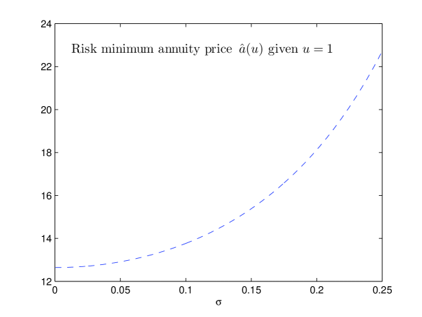
Figure 1: The profile of dependence from $\sigma$ of risk minimum annuity price $\hat{a}(u)$ given $u=1$ defined by (12) with $r=0.05$ and $T=20$.

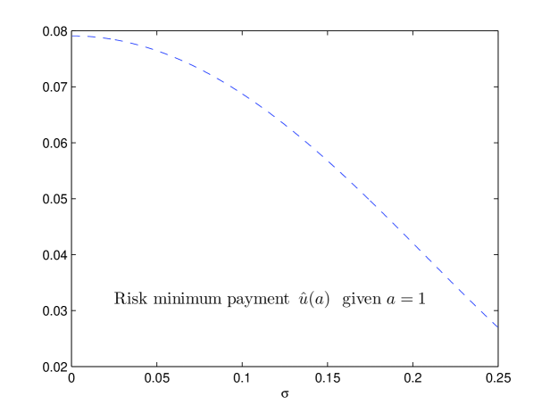
Figure 2: The profile of dependence from $\sigma$ of the risk minimum payment $\hat{u}(a)$ given $a=1$ given $u=1$’ defined by (12) with $r=0.05$ and $T=20$.

Figures 1-2 illustrate Theorem 1 for the case where $r(t)\equiv 0.05$ and $T=20$, and where $\sigma(t)\equiv\sigma$ is constant. Figure 1 illustrates Theorem 1(i) and shows the shape of dependence from $\sigma$ of the risk minimum annuity price $\hat{a}(u)$ on $\sigma$ given $u=1$ defined by (10). Figure 2 illustrates Theorem 1(ii) and shows the shape of dependence from $\sigma$ of the risk minimum payment $\hat{u}(a)$ given $a=1$ defined by (12).

Remark 1

It can be noted that maximization of the expected return for either parties is excluded from our optimization setting, because this type of maximization leads to a non-cooperative zero-sum game where the gain of one party would lead to the same loss for the counterparty; in this case, an equilibrium solution is not feasible. In our setting, both parties target minimization of the same value ${\bf E}[|a-\tilde{x}_{u}(T)|^{2}]$; this, in principle, could lead to the same equilibrium price. At least, this equilibrium price exists in the deterministic case, where (5) and (6) give the same solution for both Problems 1 and 2.

3 Impact of the presence of two different optimal solutions

Let $\widehat{a}(u)$ be optimal (risk minimum) $a$ given $u$, and let $\widehat{u}(a)$ be optimal $u$ given $a$; they are defined by (10) and (12) respectively. For the case of deterministic model with non-random $T$ and $B(t,s)$, there exists $k>0$ such that $\widehat{a}(u)=ku$ and $\widehat{u}(a)=k^{-1}a$; in other words,

$$\frac{\widehat{u}(a)}{a}=\frac{u}{\widehat{a}(u)}.$$ (19)

It does not hold for the stochastic model.

Theorem 3

If ${\rm Var\,}J(T)>0$, then

$$\frac{\widehat{u}(a)}{a}<\frac{u}{\widehat{a}(u)}.$$ (20)

It can be noted that if either $B(t,s)$ is random and $T$ is non-random, or $T$ is random and $B(t,s)$ is non-random, then ${\rm Var\,}J(T)>0$.

According to Theorem 3, the relative price of annuity is larger for the setting of Problem 1 then for the setting of Problem 2. Respectively, the rate return on the annuity investment is smaller for the setting of Problem 1 then for the setting of Problem 2.

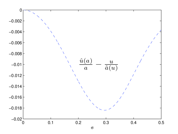
Figure 3: The profile of dependence from $\sigma$ of the difference $\frac{\widehat{u}(a)}{a}-\frac{u}{\widehat{a}(u)}$ with $r=0.05$ and $T=20$.

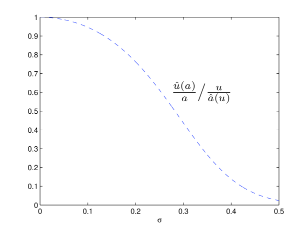
Figure 4: The profile of dependence from $\sigma$ of the ratio $\frac{\widehat{u}(a)}{a}\bigl{/}\frac{u}{\widehat{a}(u)}$ with $r=0.05$ and $T=20$.

Inequality (20) is illustrated by Figures 3-4. Figure 3 shows the shape of dependence from $\sigma$ of the difference $\frac{\widehat{u}(a)}{a}-\frac{u}{\widehat{a}(u)}$. It can be seen from this figure that the value of $\frac{\widehat{u}(a)}{a}-\frac{u}{\widehat{a}(u)}$ vanishes for larger $\sigma$. This can be explained by the fact that $\widehat{u}(a)$ with given $a$ decreases when $\sigma$ increases and that $\widehat{a}(u)$ with given $u$ increases when $\sigma$ increases. Figure 4 shows the dependence from $\sigma$ for the ratio $\frac{\widehat{u}(a)}{a}\Bigl{/}\frac{u}{\widehat{a}(u)}$. It can be seen that this value is separated from 1 even for larger $\sigma$.

For Figures 3-4, we assumed again that $r=0.05$ and $T=20$, similarly to Figures 1-2.

Economic interpretation and annuity puzzle

Theorem 3 implies that, even in our simple model, there is no a fair price that is optimal for the annuity seller as well as for annuitant, or an ”equilibrium” price. As can be seen from Figures 3-4, there is a spread between risk minimum prices calculated with different selection of what is fixed initially, $u$ or $a$. This may contribute to the explanations of the so-called ”annuity puzzle”: a statistically confirmed fact that people does not choose annuity and opt for the lump sum even given that this decision appears to contradict standard theoretical analysis; see the references provided in Section 1.

Let us consider the following Examples 1–2. For these examples, we assume, in the framework of our model, that $\sigma(t)\equiv 0.2$ and $r(t)\equiv 0.05$.

Example 1

Assume that a potential annuitant wishes to convert her life savings, $a=\$100,000$, into a term annuity for 20 years. A potential seller calculates the optimal rate of payments as $\widehat{u}(a)=\$4,206$ solving Problem 2 via (12), and will consider a larger rate of payments to be unfair. However, the potential annuitant calculates that this rate of payments would require optimal investment of $\widehat{a}(\$4,206)=\$76,242$ only, solving Problem 1 via (10). This means that there is a spread between rational annuitization prices for the customer and producer. This may lead to a disagreement about the conditions of the contract and the failure of the deal.

Example 2

Similarly, assume, that, for the same model, a seller offers an annuity with the payment rate $u=\$5,000$ for 20 years. A potential annuitant calculates the optimal price $\widehat{a}(u)=\$90,635$ solving Problem 1 via (10), and will consider a larger price to be unfair. However, the seller calculates that the investment of this size should ensure the rate of payments $\widehat{u}(\$90,635)=\$3,812$ only, solving Problem 2 via (12). Again, this may lead to a disagreement about the price and the failure of the deal.

These spreads between prices can lead to a market failure, when there is no sufficient supply for the prices acceptable for the customer.

Remark 2

We presume that it is more typical that an annuity buyer has a certain fixed amount of pension money to invest and shops for a fair annuity rate found as the solution of Problem 2 rather than target a preselected rate of payments and selecting a fair lump sum that buys it according to Problem 1. Otherwise, the situations described in Examples 1 and 2 will be reversed.

4 Proofs

The proofs below are rather technical; they use some basic facts from stochastic analysis, namely formulae for expectations of the Itô’s integrals; see, e.g., a review in Dokuchaev (2007).

Proof of Theorem 1. It follows from (1) that

$$B(t,s)=\exp\left[\int_{s}^{t}r(\tau)d\tau-\frac{1}{2}\int_{s}^{t}\sigma(\tau)^{2}d\tau+\int_{s}^{t}\sigma(\tau)dw(\tau)\right].$$ (21)

(i) The function $V(a,u)={\bf E}|\tilde{x}_{u}(T)-a|^{2}$ can be rewritten as

$$V(a,u)=u^{2}{\bf E}[J(T)^{2}]-2au{\bf E}J(T)+a^{2}.$$ (22)

Hence

$$V(a,u)=(a-u{\bf E}J(T))^{2}+R_{1}(u),$$ (23)

where

$$R_{1}(u)=u^{2}{\bf E}[J(T)^{2}]-u^{2}({\bf E}J(T))^{2}=u^{2}{\rm Var\,}J(T).$$ (24)

For a given $a$, the function $V(a,u)$ has the only minimum at $\widehat{a}(u)$ given by (10), and $V(\widehat{a}(u),u)=R_{1}(u)$.

(ii) Similarly to (23), the function $V(a,u)={\bf E}|\tilde{x}_{u}(T)-a|^{2}$ can be rewritten as

$$V(a,u)=\left(u({\bf E}[J(T)^{2}])^{1/2}-\frac{a{\bf E}J(T)}{({\bf E}[J(T)^{2}])^{1/2}}\right)^{2}+R_{2}(a),$$ (25)

where $R_{2}(a)$ is defined by (13). For a given $a$, the function $V(a,u)$ has the only minimum at $\widehat{u}(a)$ given by (12), and $V(u,\widehat{u}(a))=R_{2}(a)$. This completes the proof of statement (ii) and Theorem 1.

Proof of Corollary 1. Since $T$ is independent from $w(\cdot)$, it follows that

$${\bf E}J(T)={\bf E}[{\bf E}\{J(T)|T\}]={\bf E}y(T),\quad{\bf E}J(T)^{2}={\bf E}[{\bf E}\{J(T)^{2}|T\}]={\bf E}z(T).$$ (26)

The the statement of the Corollary follows.

Proof of Theorem 2. Let $\rho=r-\sigma^{2}/2$. By (21), we obtain that, for non-random $T$,

$$y(T)={\bf E}\left[\int_{0}^{T}B(t,0)^{-1}dt\right]={\bf E}\left(\int_{0}^{T}e^{-\rho t-\sigma w(t)}dt\right)={\bf E}\int_{0}^{T}e^{-\rho t-\sigma w(t)}dt$$

$$={\bf E}\int_{0}^{T}e^{-\rho t+\sigma^{2}t/2}={\bf E}\int_{0}^{T}e^{-rt+\sigma^{2}t}=\frac{1-e^{(-r+\sigma^{2})T}}{r-\sigma^{2}}.$$ (27)

Then (16) follows. Further, we have that, for non-random $T$,

$$z(T)={\bf E}\left[\left(\int_{0}^{T}B(t,0)^{-1}dt\right)^{2}\right]={\bf E}\left(\int_{0}^{T}e^{-\rho t-\sigma w(t)}dt\right)^{2}$$

$$={\bf E}\int_{0}^{T}\int_{0}^{T}e^{-\rho(t+s)-\sigma[w(t)+w(s)]}dtds=2{\bf E}\int_{0}^{T}dt\int_{0}^{t}e^{-\rho(t+s)-\sigma[w(t)+w(s)]}ds$$

$$=2{\bf E}\int_{0}^{T}dt\int_{0}^{t}e^{-\rho(t+s)-\sigma w(s)}{\bf E}\{e^{-\sigma w(t)}|{\cal F}_{s}\}ds.$$ (28)

For $s<t$, we have ${\bf E}\{e^{-\sigma(w(t)}|{\cal F}_{s}\}=e^{-\sigma w(s)}e^{\sigma^{2}(t-s)/2}$ and

$$z(T) = 2{\bf E}\int_{0}^{T}dt\int_{0}^{t}e^{-\rho(t+s)-\sigma w(s)}e^{-\sigma w(s)}e^{\sigma^{2}(t-s)/2}ds$$ (29)

$$= 2\int_{0}^{T}dt\int_{0}^{t}e^{-\rho(t+s)}e^{2\sigma^{2}s}e^{\sigma^{2}(t-s)/2}ds.$$

Taking the last integral, we obtain that

$$z(T)=2\int_{0}^{T}dt\int_{0}^{t}e^{t(-\rho+\sigma^{2}/2)}e^{s(-\rho+2\sigma^{2}-\sigma^{2}/2)}ds$$

$$=2\int_{0}^{T}dt\int_{0}^{t}e^{(-r+\sigma^{2})t}e^{s(-r+\sigma^{2}/2+2\sigma^{2}-\sigma^{2}/2)}ds=2\int_{0}^{T}dte^{(-r+\sigma^{2})t}\int_{0}^{t}e^{s(-r+2\sigma^{2})}ds$$

$$=2\int_{0}^{T}e^{(-r+\sigma^{2})t}\frac{1-e^{(-r+2\sigma^{2})t}}{r-2\sigma^{2}}dt.$$ (30)

Hence

$$z(T) = \frac{2}{r-2\sigma^{2}}\left[\frac{1-e^{(-r+\sigma^{2})T}}{r-\sigma^{2}}-\frac{1-e^{(-2r+3\sigma^{2})T}}{2r-3\sigma^{2}}\right]$$ (31)

$$= \frac{2}{r-2\sigma^{2}}\left(y(T)-\frac{1-e^{(-2r+3\sigma^{2})T}}{2r-3\sigma^{2}}\right).$$

Then (17) follows. This completes the proof of Theorem 2. $\Box$

Proof of Theorem 3. By Theorem 1 and by independence of $T$ from $B(t,s)$, it follows that

$$\widehat{a}(u)=u{\bf E}y(T)=u{\bf E}J(T),\quad\widehat{u}(a)=a\frac{{\bf E}y(T)}{{\bf E}z(T)}=a\frac{{\bf E}J(T)}{{\bf E}(J(T)^{2})}.$$ (32)

Clearly, ${\bf E}[J(T)^{2}]\geq({\bf E}J(T))^{2}$, and if ${\bf E}J(T)^{2}=({\bf E}J(T))^{2}$ then ${\rm Var\,}J(T)=0$. It follows that

$$\frac{\widehat{u}(a)}{a}=\frac{{\bf E}J(T)}{{\bf E}(J(T)^{2})}<\frac{{\bf E}J(T)}{({\bf E}[J(T)])^{2}}=\frac{1}{{\bf E}J(T)}=\frac{u}{\widehat{a}(u)}.$$ (33)

This completes the proof of Theorem 3. $\Box$

5 Discussion

The paper analyzes pricing method based on minimization of the risk associated with annuitization and caused by uncertainties in future bank rates and life longevity. The paper points out on the existence of two different versions of this problem: the risk minimizing selection of the annuity price given the size of the regular payments, and the risk minimizing selection of the size of the regular payments given the amount originally invested into the annuity. We found that, under uncertainty, these two problems have different solutions, even given that they both minimize the same value (7). So far, this feature has been overlooked in the existing literature. The gap between these two solutions for the customer and producer may contribute to the so-called annuity puzzle. In particular, customers might regard the (risk-minimizing) payment stream $\widehat{u}$, offered by a life insurance company for a given price $a$, as being too low. Similarly, producers might regard the risk-minimizing payment $\widehat{a}$ offered by the customer as being too low. This adds to the set of arguments identifying reasons for lacking annuity demand and why the annuity market is thin.

The approach suggested in the paper allows further development in several directions.

First, it would be interesting to investigate if this feature holds for more advanced models with multiple investments assets and transaction costs. The particular model presented in this paper is relatively simple and yet it captures the presence of the gap between rational prices for the producer and customer. Our conjecture is that this feature will hold for other market models and for other risk measures.

Second, it would be interesting to investigate discrete time models and impact of time discretization on the pricing formulae.

Finally, it would be interesting to reverse the pricing formulae for the sake of inference of the market parameters presented in these pricing formulae from the observed annuities prices. This would follow a classical approach where the inference of the volatility of the stock prices is reduced to calculation of the implied volatility from the inverted Black-Scholes pricing formula applied to stock option prices. Examples of extensions of this approach can be found in Dokuchaev (2018) and Hin and Dokuchaev (2016a,b). So far, the implied market parameters for the annuities market have not been considered in the literature.

References

- [1] Ameriks, J., Caplin, A., Laufer, S., van Nieuwerburgh, S. (2011). The joy of giving or assisted living? Using strategic surveys to separate public care aversion from bequest motives. Journal of Finance 66, 519–561.
- [2] Benartzi, S., Previtero, A., Thaler, R.H. (2011). Annuitization puzzles.Journal of Economic Perspectives 25, 143–164.
- [3] Brown, J.R., Kling, J.R., Mullainathan, S., Wrobel, M.V. (2008). Why don’t people insure late-life consumption? a framing explanation of the under-annuitization puzzle. The American Economic Review 98, 304-309.
- [4] Brunner, J., Pech, S. (2006). Adverse selection in the annuity market with sequential and simultaneous insurance demand. The GENEVA Risk and Insurance Review 31, 111–146.
- [5] Bütler, M., Teppa, F. (2007). The Choice Between an Annuity and a Lump Sum: Results from Swiss Pension Funds. Journal of Public Economics 91 (10), 1944–1966.
- [6] Choi, S. and Mattila, A.S. (2003). Hotel revenue management and its impact on customer’ perceptions of fairness. Journal of Revenue and Pricing Management, 2(4): 303-10.
- [7] Chung, J.Y.. (2017) Price fairness and PWYW (pay what you want): a behavioral economics perspective. Journal of Revenue and Pricing Management 16:1, 40-55.
- [8] Crawford, T., de Haan, R., and Runchey, C. (2008). Longevity risk quantification and management: a review of relevant literature. The Society of Actuaries.
- [9] Devlin, J.F., Roy, S.K., and Sekhon, H. (2014) Perceptions of fair treatment in financial services. European Journal of Marketing 48 7/8, 1315-1332.
- [10] Dokuchaev N.G. (2007). Mathematical finance: core theory, problems, and statistical algorithms. Routledge, London and New York.
- [11] Dokuchaev, N. (2018). On the implied market price of risk under the stochastic numéraire. Annals of Finance 14 223–251.
- [12] Finkelstein, A., Poterba, J. (2004). Adverse selection in insurance markets: Policyholder evidence from the U.K. annuity market. Journal of Political Economy 112, 183–208.
- [13] Gerber, H.U. (1997). Life Insurance Mathematics. Life insurance mathematics. 3rd ed. Berlin, Springer.
- [14] Hin, Lin Yee and Dokuchaev, N. (2016a). Computation of the implied discount rate and volatility for an overdefined system using stochastic optimization. IMA Journal of Management Mathematics, 27 (4), 505–527.
- [15] Hin, Lin-Yee and Dokuchaev, N. (2016b). Short rate forecasting based on the inference from the CIR model for multiple yield curve dynamics. Annals of Financial Economics 11, 1650004 (33 pages).
- [16] Horneff, W.J., Maurer, R.H., Mitchell, O.S., Stamos, M.Z., (2009). Asset allocation and location over the life cycle with investment-linked survival-contingent payouts. Journal of Banking & Finance 33, 1688–1699.
- [17] Kienzler, M. (2018) Value-based pricing and cognitive biases: An overview for business markets. Industrial Marketing Management 68, 86-94.
- [18] Kimes, S. E., Chase, R.B., Noone, B.N., and Wirtz, J. (2003), ?Perceived Fairness of Revenue Management in the US Golf Industry,? Journal of Revenue and Pricing Management, 1 (4), 322-344.
- [19] Milevsky, M. (1997). The Present Value of a stochastic perpetuity and the Gamma distribution, Insurance: Mathematics and Economics. Vol. 20 (3), 243-250.
- [20] Mitchell, O., Poterba, J., Warshawsky, M., Brown, J. (1999). New evidence on the money’s worth of individual annuities. American Economic Review 89(5), 1299-1318.
- [21] Pang, G., Warshawsky, M. (2010). Optimizing the equity-bond-annuity portfolio in retirement: The impact of uncertain health expenses. Insurance: Mathematics and Economics 46, 198–209.
- [22] Schreiber, P., Weber, M. (2013). Time Inconsistent Preferences and the Annuitization Decision. Working paper: http://ssrn.com/abstract=2217701.
- [23] Schweizer, M. (2001). A guided tour through quadratic hedging approaches. In: E. Jouini, J. Cvitanic, M. Musiela (eds.), Option Pricing, Interest Rates and Risk Management, Cambridge University Press, 538-574.
- [24] Tennebein, A., Vanderhooof, I.T., (1980). New mathematical laws of select and ultimate mortality. Transactions of the Society of Actuaries 32, 119–158.
- [25] Xia, L., Monroe, K.B., Cox, J.L. (2004) The Price Is Unfair! A Conceptual Framework of Price Fairness Perceptions. Journal of Marketing Vol. 68, No. 4, pp. 1-15
- [26] Yaari, M. (1965). Uncertain Lifetime, Life Insurance and the Theory of the Consumer. The Review of Economic Studies, 32(2), 137-150.
- [27] Zhan, L. and Lloyd, A.E.. (2014) Customers’ asymmetrical responses to variable pricing. Journal of Revenue and Pricing Management. 13:3, 183-198.