Smooth or shock: universality in closed inhomogeneous driven single file motions

Abstract

We study the nonequilibrum steady states in a unidirectional or driven single file motion (DSFM) of a collection of particles with hard-core repulsion in a closed system. For driven propulsion that is spatially smoothly varying with a few discontinuities, we show that the steady states are broadly classified into two classes, independent of any system detail: (i) when the steady state current depends explicitly on the conserved number density $n$, and (ii) when it is independent of $n$. This manifests itself in the universal topology of the phase diagrams and fundamental diagrams (i.e., the current versus density curves) for DSFM, which are determined solely by the interplay between two control parameters $n$ and the minimum propulsion speed along the chain. Our theory can be tested in laboratory experiments on driven particles in a closed geometry.

Directed single file motion (DSFM) implies unidirectional particle movement along narrow channels where the particles cannot cross each other due to hardcore repulsion. It is an inherently nonequilibrium process that consumes energy for propulsion. We are particularly interested in DSFM with spatially nonuniform propulsion and finite resources, i.e., fixed available number of particles. This should be relevant in wide-ranging systems, e.g., vehicular or pedestrian movement along closed network of roads with bottlenecks having varying strength, closed urban transport networks with enforced speed variations traffic ; traffic2 and spatially varying electric fields in closed arrays of quantum dots qdot . This study could form the basis for further research on weakly number conserving quasi one-dimensional (1D) transport models where particle number conservation approximately holds at time-scales shorter than any nonconserving processes; e.g., ribosome translocations along closed mRNA loops with pause sites (for which ribosomes are typically re-initiated in translocation and breaking of ribosome number conservation is likely to affect only at relatively large time scales) zia1 ; ribo ; pause1 . It should also be useful in studies on the effects of quenched disorder on asymmetric exclusion processes with finite resources zia .

The general goal of this work is to theoretically understand the classes of steady states in spatially nonuniform systems with restricted one-dimensional (1D) motion with finite resources, and to elucidate their universal nature. For this, we construct a minimal theory for DSFM with position-dependent propulsion speed and hardcore repulsion in closed geometries, with the total number of particles $N_{tot}$ being conserved. This theory adequately describes the interplay between inhomogeneity and conservation laws, and reveals the generic universal nature of the nonequilibrium steady states. It applies to all in-vitro or in-vivo systems where individual particles are non-active or weakly active, i.e., do not actively push or pull the neighbors strongly and are undergoing quasi-1D motion, without mutual passage and having number conservation. It can also be useful and serve as theoretical benchmark for quasi-1D systems with weak particle non-conservation, e.g., binding factor mediated enhancement of the probability of loop formation in mRNA in eukaryotes chou1 . The results can be tested in carefully designed in-vitro experiments on the collective motion of driven particles along a nonuniform closed track.

We focus on the steady state densities in DSFM and their dependences on $N_{tot}$ and position-dependent propulsion. In order to extract generic results from a minimal description without losing the essential physics, we model DSFM by the well-known 1D totally asymmetric simple exclusion process (TASEP), where each site can accommodate at most one particle that can hop only in one direction if the neighboring site is empty. TASEP with open boundaries is a simple model for nonequilibrium phase transitions in 1D open systems derrida ; krug-ori ; zia1 .

In this article, we study closed TASEP with $N$ sites as a model for DSFM. Space-dependent propulsion is described by quenched hopping rates that are spatially smoothly varying with finite number of discontinuities having single or multiple point minima. The main results are: (i) independent of the details of the heterogeneous hopping rates, there are generically two classes of steady states delineated by the steady state current $J$: (a) when $J$ depends on mean density $n=N_{tot}/N$ ($0<n<1)$ explicitly (hereafter smooth phase), and (b) when $J$ is independent of $n$, characterized by a phase separation with localized (LDW) or delocalized (DDW) domain walls (hereafter shock phase), (ii) the phases and the reentrant transitions between them are controlled by the interplay between $n$ and the global minima $q_{min}$ of the position-dependent propulsion speed, (iii) moving shocks appear only for multiple global minima in propulsion speed; multiple local minima with only one global minimum only produce a localized shock, and (iv) while accumulation of particles where the hopping rate is low is naïvely expected, we show below that the position of the peak of the density in the shock phase can actually be anywhere in the system, being controlled by $n$.

This article shows how the general concept of universality, well-developed for equilibrium systems, applies for spatially-varying steady state density profiles in driven inhomogeneous systems with number conservation. This remains hitherto unexplored. More specifically, the topology of the phase diagrams plotted as functions of $n$ and $q_{min}$ and the associated fundamental diagrams (i.e., the $J$ versus $n$ plots) is argued to be universal, independent of the precise hopping rate functions; see Fig. 1.

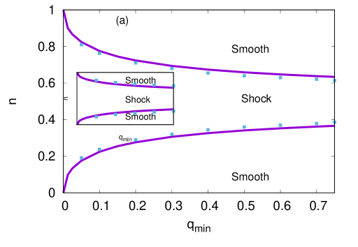
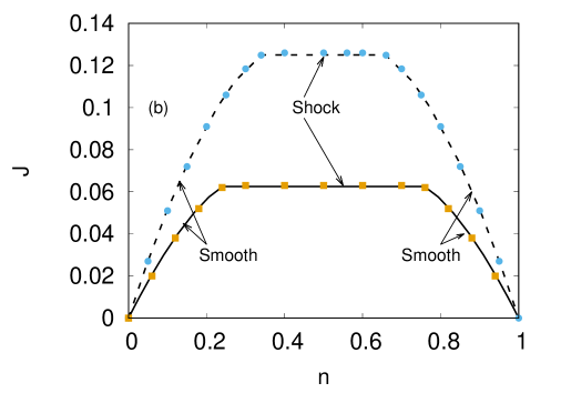
Figure 1: (a) Illustrations of universal topology of the phase diagrams in the $q_{min}-n$ plane: (i) $q(x)=(x-0.5)^{2}+q_{min}=q_{1}(x)$, and (ii) (inset) $q(x)=0.5x^{2}+q_{min}=q_{2}(x)$ (with $n=[0,1]$ and $q_{min}=[0,0.75]$). The range of $q_{min}$ is chosen in such a way that $q(x)$ does not exceed unity anywhere. Magenta lines and blue points are overlapping MFT and MCS results, respectively. (b) Fundamental diagrams ($J$ vs $n$) for $q_{1}(x)=(0.5-x)^{2}+0.5$ (dashed curves) and $q_{2}(x)=0.5x^{2}+0.25$ (solid curves) as chosen above for (a). The different phases that exist on the fundamental diagrams are marked. Both curves have the same form (see text). Note the saturation of current $J$ with respect to the density $n$ in the shock phase. Curves and points represent MFT and MCS results, respectively.

The model has a hopping rate $q_{i}\leq 1$ at a site $i$. The dynamics clearly conserves the total particle number $N_{tot}=\sum_{i}^{N}n_{i}$, where $n_{i}$ is the occupation of site $i$. The dynamics of TASEP is formally given by rate equations for every site, which are not closed tasep . In mean-field theory (MFT), we write down the dynamical equations for TASEP in closed forms, amenable to analytical treatments. We label the sites by $x=i/N$; in the thermodynamic limit $N\rightarrow\infty$, $x$ effectively becomes a continuous variable confined between $0$ and $1$. In this parametrization, the hopping rate function is given by $0<q(x)\leq 1$; we assume $q(x)$ to be piece-wise continuous, smooth, slowly varying functions of $x$ with a few point minima. Further, we define $\rho(x)=\langle n_{i}\rangle$ as the density at $x$; here $\langle...\rangle$ refers to temporal averages in the steady states. Studies on quenched heterogeneous TASEP has a long history; see, e.g., Refs. mustansir ; stinchcombe ; others ; shaw for some studies on different aspects of heterogeneous TASEP. Our model complements these existing works, and primarily investigates the notion of universality not discussed elsewhere.

In the steady states

$$\frac{\partial\rho}{\partial t}=-\frac{\partial}{\partial x}[q(x)\rho(1-\rho)]=0,$$ (1)

in MFT over a range of $x$ in which $q(x)$ is smooth  erwin-rev . This gives

$$q(x)\rho(x)[1-\rho(x)]=J,$$ (2)

where $J$, a constant (yet unknown) is the steady state current. Equation (2) has two spatially nonuniform solutions $\rho_{+}(x)$ and $\rho_{-}(x)$:

$$\rho_{+}(x) = \frac{1}{2}\left[1+\sqrt{1-4J/q(x)}\right]>\frac{1}{2},$$ (3)

$$\rho_{-}(x) = \frac{1}{2}\left[1-\sqrt{1-4J/q(x)}\right]<\frac{1}{2},$$ (4)

for all $x$. Clearly, both $\rho_{+}(x)$ and $\rho_{-}(x)$ are smooth functions for all $x$, except where $q(x)$ itself is discontinuous. Since $\rho(x)>0$ for all $x$, $1-\frac{4J}{q(x)}\geq 0$. Thus

$$J\leq q(x)/4,$$ (5)

everywhere. The maximum allowed value of $J$ is thus independent of $n$:

$$J_{{max}}=q_{min}/4,$$ (6)

whence $\rho_{+}(x_{0})=\rho_{-}(x_{0})$; $x=x_{0}$ is the location of $q_{\rm min}$; see Ref. krug-brazi for analogous result in a disordered exclusion model.

We now outline the derivation of the results announced in the beginning of this article and the principles for the construction of Fig. 1, followed by some illustrations of the phases for some representative $q(x)$. Since $\rho_{+}(x)(\rho_{-}(x))>(<)1/2$ for all $x$ except at isolated points $x_{0}$ where $q(x)=q_{min}$, for a given $q(x)$ if $n$ is sufficiently close to 1/2, $\rho(x)$ must be a combination of $\rho_{+}(x)(>\frac{1}{2})$ and $\rho_{-}(x)(<\frac{1}{2})$. This is the shock phase mentioned above. In contrast, when $n$ approaches 0, there are only a few particles in the system and $\rho(x)=\rho_{-}(x)$ in the steady state throughout the system. Analogously, for $n$ approaching unity, $\rho(x)=\rho_{+}(x)$ in the steady state. The smooth phases with $\rho(x)=\rho_{-}(x)<1/2$, and $\rho(x)=\rho_{+}(x)>1/2$ are spatially nonuniform, and hence generalize the spatially uniform low density (LD) and high density (HD) phases, respectively, of TASEP with open boundaries erwin-rev . Thus, a re-entrant smooth-shock-smooth nonequilibrium phase transition is expected as $n$ rises from 0 to 1 for any given $q(x)$. The precise boundaries between these phases for a given $n$ and $q(x)$ - which will tell us for a given $q(x)$ how close $n$ must be to 1/2 for the smooth-shock transition - are obtained by imposing particle number conservation on (3-4) and using (6); see below.

Current $J$ is fixed by the particle number conservation:

$$\int_{0}^{1}\rho_{a}(x)=n,\;a=+\,-.$$ (7)

From (3) and (4), the maximum (minimum) of $\rho_{-}(x)$ ($\rho_{+}(x)$) coincides with the minimum of $q(x)$, a fact borne out by our Monte-Carlo Simulation (MCS) studies: $q_{min}$ effectively acts as a bottleneck, and as a result, particles tend to accumulate behind it (see below).

As $n$ increases from zero, $J$ rises and eventually reaches $J_{max}$. For $J=J_{max}$, $\rho_{+}(x_{0})=\rho_{-}(x_{0})$, where $x_{0}$ is the location of $q_{min}$. On increasing $n$ further, the additional particles are accommodated by representing $\rho(x)$ as a combination of $\rho_{-}(x)$ and $\rho_{+}(x)$ which meet smoothly at $x_{0}$. Since particles should accumulate behind the bottleneck at $x_{0}$, we expect that additional particles will go over to the high density solution represented by $\rho_{+}(x)$. Since we have a closed system, the two solutions must meet at another point $x_{w}$, such that $\rho_{+}(x_{w})>\rho_{-}(x_{w})$ (since $\rho_{+}(x)=\rho_{-}(x)$ only at $x=x_{0}$), leading to a discontinuous jump in the form of a localized domain wall (LDW) in $\rho(x)$ at $x_{w}$, thus giving rise to the shock phase, with a jump $\overline{\rho}$ given by

$$\rho_{+}(x_{w})-\rho_{-}(x_{w})=\overline{\rho},$$ (8)

controlled by $n$ and the functional form of $q(x)$. As more particles are added, $x_{w}$ shifts to make the region of existence for $\rho_{+}(x)$ larger and $\rho_{-}(x)$ smaller. This indeed leaves $J=J_{max}=q_{min}/4$ unchanged. Thus the current in the shock phase saturates to its maximum value $J_{max}$. This continues till $\rho_{+}(x)$ spans the full system. Thus, as $n$ rises from the low to moderate values, a smooth-to-shock transition is encountered. Interestingly, independent of the form of $q(x)$ this transition is reentrant - since, as $n$ rises further, the system moves from shock phase to smooth phase again, with $\rho_{+}$ now being the only valid solution. This reentrant transition can also be understood from the particle-hole symmetry of the model. Since particle density $\rho_{+}(x)$ can be interpreted as the hole density $1-\rho_{+}(x)=\rho_{-}(x)$, if $\rho_{-}(x)$ is a steady state solution for overall particle density $n$, $\rho_{+}(x)$ is a steady state solution for particle density $1-n$. This picture remains valid even when there are additional local minima (but only one global minimum $q_{min}$ at $x_{0}$): $J_{max}$ is still controlled solely by $q_{min}$ [Eq. (6) above], with $\rho_{+}(x_{0})=\rho_{-}(x_{0})$; the other local minima having no effect on $J_{max}$ are effectively screened in any steady state current measurements in shock phase. However, the form of the LDW, i.e., the functional form of $\rho(x)$, depends on any local minima through its dependence on the full form of $q(x)$.

Assuming only one global minimum for $q(x)$, at the phase boundary between smooth and shock phases, $J=J_{max}=q_{min}/4$ and $\rho(x)=\rho_{-}(x)$ (for $n<1/2$) for all $x$, or for $n>1/2$, $\rho_{+}(x)$ for all $x$. Thus

$$\int_{0}^{1}dx\rho_{\pm}(x,J_{max}) = \int_{0}^{1}dx\frac{1}{2}[1\pm\sqrt{1-\frac{q_{min}}{q(x)}}]=n,$$ (9)

give the quantitative dependence of $n$ on $q_{min}$ for the re-entrant transition, or equivalently, the boundaries between smooth and shock phases in Fig. 1 (a). As our arguments above are independent of the precise form of $q(x)$, the topology of the phase diagrams in Fig. 1 (top) should remain independent of the precise forms of $q(x)$ having same $q_{min}$. This is the universality in DSFM mentioned in the beginning that is also manifest in the fundamental diagrams in Fig. 1 (bottom), obtained from (2) and (7). The results in Fig. 1 are also obtained from the MCS studies, that corroborate the MFT predictions closely. This holds true even if there are multiple global minima with value $q_{min}$; in this case, shock phases correspond to moving shocks (see below). Notice that the topology of the phase diagram and the corresponding fundamental diagram are same as those obtained in Ref. lebo , where a single slow site controls the current, establishing an equivalence between the model of Ref. lebo with a single slow site and our model here. The strength of the single slow site in the model of Ref. lebo corresponds to $q_{min}$ here.

We now illustrate the phases with few representative choices for $q(x)$. See Fig. 2 for a plot of $\rho(x)$ versus $x$ in the smooth phase; see also Figs. (7-9) in Appendix for plots of $\rho(x)$ with different $q(x)$ in the smooth phase; good agreements between MFT and MCS results are evident.

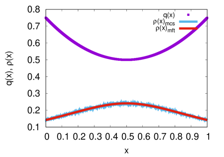
Figure 2: Plot of $\rho(x)$ versus $x$ in the LD phase ($n=0.2$). Magenta line indicates the hopping rate function $q(x)=(x-0.5)^{2}+0.5$. Red continuous line and blue points denote $\rho_{-}(x)$, respectively, from MFT and MCS studies (see text). Excellent agreement between MFT and MCS results is clearly visible. We have used $N=2000$.

Further see Fig. 3 for a plot of the density in the shock phase for a choice of $q(x)$, again showing strong agreements between MCS and MFT results; see also Fig. 10 in Appendix.

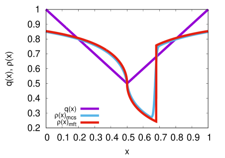
Figure 3: Plot of $\rho(x)$ versus $x$ in the shock phase with $n=0.7,N=2000$. Magenta line indicates $q(x)=1-x,0\leq x<0.5$ and $q(x)=x,0.5\leq x<1$. Red line and blue points, respectively, represent MFT and MCS results for $\rho(x)$.

Notice that the peak of the density in the smooth phase in Fig. 2 coincides with the location of $q_{min}$. As argued above, this can be understood from the form of $\rho_{-}(x)$ as given in (4) - clearly, the maximum of $\rho_{-}(x)$ must coincide with the minimum of $q(x)$. In contrast, the location of the extrema of the density profiles in the shock phase have no such relation with the minimum of $q(x)$. Instead, as we note in Fig. 3, $\rho(x)$ is continuous at the location $x_{0}$ of $q_{min}$, so long as $q(x)$ itself is continuous at $x_{0}$ (since $\rho_{+}=\rho_{-}$ at $x_{0}$). If however, $q(x)$ itself is discontinuous at $x_{0}$, the density is also discontinuous there; see Fig. 10 (right) in Appendix. In both these cases, the density has a discontinuity elsewhere whose location is controlled by $n$ for a given $q(x)$ with $q(x)$ being continuous there. This is one of the principal results in this article. Furthermore, given that $\rho_{+}(x)$ reduces and $\rho_{-}(x)$ grows when $q(x)$ grows in $x$ [see Eqs. (3) and (4) above], the density in the shock phase being a linear combination of $\rho_{+}(x)$ and $\rho_{-}(x)$, can have a peak anywhere in the system that is controlled by $n$.

We further illustrate the occurrence of a single LDW in the shock phase with $q(x)$ having multiple local but one global minimum in Fig. 4, with $\rho_{+}(x)=\rho_{-}(x)$ only at the location of the global minimum of $q(x)$, in agreement with the theoretical predictions.

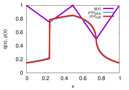
Figure 4: One LDW with $n=0.6,N=2000$ and $q(x)=1-x$, $x=[0,0.25]$; $q(x)=0.5+x$, $x=[0.25,0.5]$; $q(x)=2-2x$, $x=[0.5,0.75]$; $q(x)=2x-1$, $x=[0.75,1]$ with two local minima of $q(x)$ at x = 0.25 and x = 0.75. Excellent agreement between MFT and MCS is observed.

When there are multiple global minima, the above-mentioned theory of LDW breaks down and very different physics emerges in the shock phase. For instance, consider $q(x)$ to have only two global minima at diametrically opposite points $x_{1}$ and $x_{2}$: $q(x_{1})=q(x_{2})=q_{min}$, see Fig. 5 for such a choice of $q(x)$. Thus there are now two effective bottlenecks at $x_{1}$ and $x_{2}$ which split the ring into two identical segments, say $T_{A}$ and $T_{B}$ frey ; niladri1 , of equal length. Furthermore, from (3) and (4) we have

$$\rho_{-}(x_{1})=\rho_{+}(x_{1})=\rho_{-}(x_{2})=\rho_{+}(x_{2}).$$ (10)

In each of $T_{A}$ and $T_{B}$, MFT for the shock phase applies. Therefore, two domain walls are expected. Particle number conservation then can only yield a single relation between the two domain wall positions and $n$, and cannot determine both $x_{w1}$ and $x_{w2}$ separately. This means that a shift in $x_{w1}$ can be balanced by an equivalent reverse shift in $x_{w2}$ that still satisfies particle number conservation. Due to the inherent stochasticity of the system, all possible solutions of $x_{w1}$ and $x_{w2}$ that are consistent with particle number conservation are visited by the system, if waited long enough. This leads to two DDWs. Under long time averages, envelops of the moving DDWs will be observed; see Fig. 5 and Appendix for detailed calculations.

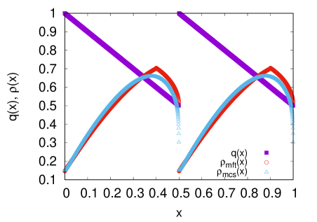
Figure 5: Plot of $\rho(x)$ versus $x$ showing two DDWs; $n=0.5$. Magenta lines indicate $q(x)=1-x,0\leq x<0.5$ and $q(x)=1.5-x,0.5\leq x<1$; red line and blue points, respectively, are MFT and MCS results for DDW, which agree with each other.

As the DDWs in Fig. 5 move, $T_{A}$ and $T_{B}$ exchange particles. Particle number conservation ensures that when a particle enters (leaves) $T_{A}$, it must necessarily leave (enter) $T_{B}$, leading to perfect synchronization of the DDWs in $T_{A}$ and $T_{B}$; see Appendix for additional discussions and an associated kymograph in Fig. 6.

If there are more than two global minima of $q(x)$, then there will be as many sub-channels ($T_{A},T_{B},T_{C}...$), and thus, as many DDWs. However, the argument for synchronization breaks down in such cases; thus there should be no synchrony in movement between any two of the DDWs; see Fig. 11 (left) (and the corresponding kymograph Fig. 11 (right)) and related discussions in Appendix.

The shocks in open TASEPs, which are always delocalized, appear when the entry ($\alpha$) and exit ($\beta$) are equal and not exceeding 1/2. This is equivalent to $J_{in}=J_{out}$, where $J_{in}$ and $J_{out}$ are, respectively, the currents determined by the entry side and exit side boundaries. The shock phase of the present model is analogous to the shocks in open TASEPs. To see this we note that our ring model can be viewed as an open TASEP with effective entry ($\alpha_{e}=\rho_{-}(x_{0})$) and exit ($\beta_{e}=1-\rho_{+}(x_{0})$) rates that is joined at $x_{0}$, the location of $q_{min}$ (assuming a single global minimum) niladri1 ; frey ; tirtha1 . From the condition of the shock phase, $J_{in}=J_{out}=J_{max}=q_{min}/4$ holds automatically. That we obtain an LDW here as opposed to a DDW in an open TASEP under equivalent conditions is due to the strict particle number conservation here; see Refs. lebo ; niladri1 ; tirtha1 ; zia . When there are two or more global minima of $q(x)$, the system can be thought to consist of those many TASEPs joined together to form a ring; see Refs. niladri1 ; tirtha1 . The conditions for the shock phase is satisfied in all these TASEP segments simultaneously, leading to formation of a domain wall in each of them. As explained in Refs. niladri1 ; tirtha1 , in this situation number conservation cannot pin the domain walls completely giving rise to DDWs; see also Appendix. We lastly note one point of dissimilarity between the shocks here and the DDWs in an open TASEP: for the latter, the current is less than its maximum value, where as in the shock phase here, the current necessarily saturates at its maximum value of $J_{max}$.

We have thus developed the theory for DSFM in a closed system with position-dependent propulsion by studying a closed TASEP with quenched hopping rates $q(x)$. This theory reveals the universal form of the phase diagrams and the fundamental diagrams of the model, for generic smooth $q(x)$ with a finite number of discontinuities and global minimum, but independent of the precise forms for $q(x)$. Our theory is sufficiently general and applies to any smoothly varying $q(x)$ with finite number of discontinuities; it generalizes the analyses in Ref. stinchcombe . From the perspectives of nonequilibrium systems, these results generalize the studies in Refs. lebo ; mustansir ; stinchcombe1 ; niladri1 ; tirtha1 . In the more complex situation where individual particles can actively push (or pull) its neighbor, thus only dynamically modulating the effective hopping rate, we expect our results to remain valid for weak activity. For strong activity, competition between background heterogeneous hopping and the active processes will determine the steady state, whose full analysis is beyond the scope of the present work. We have here studied smooth $q(x)$ with a small number of discontinuities. There are in-vivo situations where $q(x)$ could be rapidly fluctuating, e.g., the DNA strands dna . It would be interesting to study to what degree our results remain valid for rapidly fluctuating $q(x)$.

Lastly, MFT developed here neglects spatial density correlations, which is an approximation. This may be improved by systematically including two-point correlations; see, e.g., Ref. shaw . It has been shown that extended particles instead of point particles significantly affect the steady state densities of an open TASEP with site-dependent hopping rate; see Refs. shaw ; dan . It will be interesting to study this effect in a closed TASEP.

This theory may be verified in model experiments on the collective motion of driven particles with light-induced activity bechinger-jphys in a closed narrow circular channel bechinger ; bechinger-rmp . Unidirectionality of the motion can be ensured by suppressing rotational diffusion, e.g., by choosing ellipsoidal particles with the channel width shorter than the long axis of the particle everywhere, or by using dimer particles. Propulsion speed can be tuned by applying patterned or spatially varying illumination bechinger-jphys . Steady state densities can be measured by microscopy with image processing. While technical challenges are anticipated in setting up appropriate experimental arrangements, we hope this will be realized in near future.

Acknowledgement:- We thank M. Khan for constructive suggestions and careful reading of the manuscript. We also thank C. Maes for his critical comments on the manuscript. The authors gratefully acknowledge partial financial support from the Alexander von Humboldt Stiftung, Germany under the Research Group Linkage Programme (2016).

Appendix A Density profiles for delocalized domain walls

We calculate here the steady state density profiles when $q(x)$ has two symmetrically placed global minima of same value. The system then can be considered to consist of two TASEP chains of equal size niladri1 , say $T_{A}$ (with $0\leq x\leq 1/2$) and $T_{B}$ (with $1/2\leq x\leq 1$), each spanning from one global minimum of $q(x)$ to the other. While the total particle number in the ring is conserved, the number of particles in each of $T_{A}$ and $T_{B}$ can fluctuate. We closely follow Ref. erwin-tobias in our analysis below.

Now consider one delocalized domain wall (DDW) in each of $T_{A}$ and $T_{B}$. Let $x_{w}^{A}$ and $x_{w}^{B}$ be the instantaneous positions of the DDWs in $T_{A}$ and $T_{B}$, respectively and the respective heights be $\Delta_{A}(x_{w}^{A})$ and $\Delta_{B}(x_{w}^{B})$. We note here that the DDW heights are explicit functions of their positions, since the steady state density is not uniform for an arbitrary $q(x)$.

Now, increasing the number of particles in $T_{A}$ by $1$ would imply shifting $x_{w}^{A}$ by an amount $\delta x_{w}^{A}=\frac{-1}{L\Delta_{A}}$. Similarly, decrease of a particle would mean $\delta x_{w}^{A}=\frac{1}{L\Delta_{A}}$. In order to understand why this is so, we note that the ’height $\Delta_{A}$ of the domain wall (DW) at $x_{w}^{A}$’ means that $\Delta_{A}$ number of excess particles are needed to fill up one lattice spacing ($=\frac{1}{L}$), or to cause one lattice spacing leftward/rightward movement of the DW (and thus, the above values of $\delta x_{w}^{A}$). Let us now note that there are two basic processes which can alter the number of particles individually in $T_{A}$ and $T_{B}$, i.e., if a particle enters $T_{A}$ through its left boundary (equivalent to a particle leaving $T_{B}$ through its right boundary) and vice-versa.

For the following analysis, we will focus on $T_{A}$. Let $P(x_{w}^{A},t)$ be the probability of finding a DW at $x_{w}^{A}$ at time $t$. For a given $x_{w}^{A}$, one can evaluate $x_{w}^{B}$ at time $t$, uniquely, using total particle number conservation. The transition rate for a particle entering $T_{A}$ through the left boundary can be written as, $W_{L}=J_{in}=q(x=0)\alpha_{e}^{A}(1-\alpha_{e}^{A}),\delta x_{w}^{A}=\frac{-1}{L\Delta_{A}}$. Similarly, the transition rate for the particle leaving through the right boundary is given by $W_{R}=J_{out}=q(x=1/2)\beta_{e}^{A}(1-\beta_{e}^{A}),\delta x_{w}^{A}=\frac{1}{L\Delta_{A}}$. Here, $\alpha_{e}$ are $\beta_{e}$ are the densities at $x=0$ and $x=1/2$, respectively, in $T_{A}$, e.g., $\alpha_{e}=\rho(x=0)$ etc.

With these transition rates, we can calculate the average shift or the expectation value of the change, $\langle\delta x_{w}^{A}\rangle$, which is given by the product of the increment (with sign) and the sum of the different transition rates:

$$\left<\delta x_{w}^{A}\right>=\frac{1}{L\Delta_{A}(x_{w}^{A})}\left[J_{out}-J_{in}\right].$$ (11)

It should be noted here, that the domain wall itself performs, a random walk about its mean position, $\overline{x_{w}^{A}}$. For the fixed point of the random walk, i.e., the value of $x_{w}^{A}$ for which $\langle\delta x_{w}^{A}\rangle=0$, we obtain,

$$J_{out}-J_{in}=0,$$ (12)

the well known condition for formation of domain walls. In order to calculate the steady state profiles of the DDWs, we need to study the fluctuations in the DW positions that we do below.

Using the expressions for the transition rates defined above, we can write down the Master equation for $P(x_{w}^{A},t)$, the probability of finding the DW at $x_{w}^{A}$ at time $t$.

$$\frac{dP(x_{w}^{A},t)}{dt} = \Sigma_{\delta x_{w}^{A}}[P(x_{w}^{A}+\delta x_{w}^{A},t)W(x_{w}^{A}+\delta x_{w}^{A}\rightarrow x_{w}^{A})$$ (13)

$$- P(x_{w}^{A},t)W(x_{w}^{A}\rightarrow x_{w}^{A}+\delta x_{w}^{A})]$$

To proceed further, we employ Kramers-Moyal expansion kramers of the Master equation above around $\overline{x_{w}^{A}}$, up to second order in $\delta x_{w}^{A}$. This gives,

$$\frac{dP(x_{w}^{A},t)}{dt}=-\frac{\partial}{\partial y}\left[a(y)P(y,t)\right]+\frac{1}{2}\frac{\partial^{2}}{\partial y^{2}}\left[b(y)P(y,t)\right],$$ (14)

where, $y=\delta x_{w}^{A}$, $a(y)=\Sigma_{y}yW(x_{w}^{A}+\delta x_{w}^{A}\rightarrow x_{w}^{A})$ and $b(y)=\Sigma_{y}y^{2}W(x_{w}^{A}+\delta x_{w}^{A}\rightarrow x_{w}^{A})$. Using the already known values for $W$ and $\delta x_{w}^{A}$, and Eq. (12) we arrive at the following results for $a$ and $b$:

$$a(x_{w}^{A})=\frac{1}{L\Delta_{A}(x_{w}^{A})}\left[-\alpha_{e}^{A}(1-\alpha_{e}^{A})+\beta_{e}^{A}(1-\beta_{e}^{A})\right]=0$$ (15)

and

$$b(x_{w}^{A})=\frac{1}{L^{2}\Delta_{A}^{2}(x_{w}^{A})}\left[\alpha_{e}^{A}(1-\alpha_{e}^{A})+\beta_{e}^{A}(1-\beta_{e}^{A})\right]>0$$ (16)

Thus up to this order

$$\frac{dP(x,t)}{dt}=\frac{1}{2}\frac{\partial^{2}}{\partial x^{2}}\left[b(x)P(x)\right].$$ (17)

Since $J_{in}=J_{out}$, the DW position effectively follows detailed balance condition. This means the fluctuations in the DW position should follow an equilibrium distribution in the steady state. Hence, the probability current, given by $J_{DW}(x)=\frac{\partial}{\partial x}\left[b(x)P(x)\right]=0$. This yields

$$P(x)=\frac{C}{b(x)},$$ (18)

where $C$ is a constant which can be evaluated by the normalization condition on $P(x)$.

A.1 Construction of the density profiles

We can now construct the density profile $\rho(x)$ with the knowledge about $P(x)$. Since the long time averaged steady state density involves averaging over $P(x)$, we argue that

$$\frac{\partial\rho}{\partial x}=AP(x),$$ (19)

where $A$ is a constant of proportionality. Clearly from Eq. (19), we can see if $P(x)={\rm const.}$, as in the case for a DDW in an open TASEP, $\rho(x)$ varies linearly with $x$, a known result. The constant $A$ in this example can be evaluated by the boundary conditions. In yet another example, for an LDW as $P(x)\propto\delta(x-x_{w})$, $\rho(x)$ is a heaviside $\Theta$-function according to Eq. (19), whose height can be determined using the boundary conditions. We now obtain the DDW steady state density profiles.

By using Eq. (19) we write

$$\rho(x)=\tilde{A}\int\frac{dx}{b(x)}+D=A_{1}\int dx(\rho_{+}(x)-\rho_{-}(x))^{2}+D,$$ (20)

where, $\tilde{A},A_{1}$ and $D$ are constants, and we have substituted the value of the DW height $\Delta_{A}(x)=\rho_{+}(x)-\rho_{-}(x)$ in $b(x)$. Using already derived expressions for $\rho_{-}(x)$ and $\rho_{+}(x)$ above, we finally arrive at the following expression for the DDW profile,

$$\rho(x)=A_{1}\int dx(1-\frac{q_{min}}{q(x)})+D.$$ (21)

The value of the constants can be fixed using the boundary conditions on $\rho(x)$. But there is one more undetermined quantity that we are yet to address. The DDW in general has certain extent of wandering in $T_{A}$ that is less than the length of the channel, depending on the number density. We can have two situations: one, where $\rho(x)$ shows a mix of LD and DDW profiles, or where it is a mix of DDW and HD profiles. Therefore, within $x=[0,1/2]$, we can either have a situation with an LD phase from $x=0$ to say, $x=\overline{x}$, followed by the DDW from $x=\overline{x}$ to $x=1/2$; or the situation with the DDW from $x=0$ to $x=\overline{x}$, followed by an HD phase from $x=\overline{x}$ to $x=1/2$. Now, what determines the value of $\overline{x}$ is the condition $\int_{0}^{1/2}\rho_{A}(x)dx=n$, where $\rho_{A}(x)$ is the complete density profile for $T_{A}$ and $n$ is the number density (notice that $T_{A}$ and $T_{B}$ are identical, and both must have the same average number density). If the DDW does not span the entire $T_{A}$, an additional unknown parameter $\overline{x}$ must be determined, which we fix numerically by using the particle number conservation. This in turn yields the complete density profile. We use this scheme to obtain $\rho(x)$ for $q(x)=1-x$ for $x=[0,0.5]$ and $q(x)=1.5-x$ for $x=[0.5,1]$; see Fig. 5 in the main text. Good agreement with the MCS result is clearly visible, establishing our analytical framework.

Appendix B Synchronization of DDW movement

We now show that the two DDWs formed when $q(x)$ has two global minimal placed at diametrically opposite points in the ring move with perfect synchrony. To do that we first consider the two basic microscopic processes in the dynamics that lead to the movement of individual domain walls.

• (i) A particle leaves $T_{A}$ and enters into $T_{B}$.

• (ii) A particle leaves $T_{B}$ and enters into $T_{A}$.

Let $\delta x_{w}^{A}$ and $\delta x_{w}^{B}$ be the shifts in the instantaneous positions $x_{w}^{A}$ and $x_{w}^{B}$ of the domain walls in $T_{A}$ and $T_{B}$, respectively, due to the processes mentioned above. Jumps in the densities at $x_{w}^{A}$ and $x_{w}^{B}$ are given by

$$\rho_{+}(x_{w}^{A})-\rho_{-}(x_{w}^{A})=\overline{\rho}_{A},\rho_{+}(x_{w}^{B})-\rho_{-}(x_{w}^{B})=\overline{\rho}_{B}.$$ (22)

In general, $\overline{\rho}_{A}\neq\overline{\rho}_{B}$.

Since $\alpha_{e}=\beta_{e}$ for both $T_{A}$ and $T_{B}$, both processes (i) and (ii) take place with equal rate $W=\alpha_{e}(1-\alpha_{e})$. By process (i) above, $\delta x_{w}^{A}=-WL^{-1}\overline{\rho}_{A}^{-1},\,\delta x_{w}^{B}=WL^{-1}\overline{\rho}_{B}^{-1}$. Similarly, by process (ii) above, $\delta x_{w}^{A}=WL^{-1}\overline{\rho}_{A}^{-1},\,\delta x_{w}^{B}=-WL^{-1}\overline{\rho}_{B}^{-1}$. Thus,

$$\langle\delta x_{w}^{A}\rangle+\langle\delta x_{w}^{B}\rangle=0$$ (23)

identically. This means $\langle\delta x_{w}^{A}\rangle=-\langle\delta x_{w}^{B}\rangle$, which is the essence of synchronization of the movements of the two DDWs in $T_{A}$ and $T_{B}$. This synchronization manifests pictorially in a kymograph given in Fig. 6.

Figure 6: Kymograph for $n=0.5,N=800$, $q(x)=1-x$ for $0\leq x<0.5;q(x)=1.5-x$ for $0.5\leq x<1$. See  tirtha1 for technical details of obtaining kymographs of the same nature in closed TASEP systems.

The above argument for synchronization breaks down when the number of global minima of $q(x)$, which is same as the number of TASEP segments that make up the ring system, exceeds two. Now imagine $q(x)$ to have $N>2$ global minima of value $q_{min}$, placed at equal spacing. Thus the ring system can now be considered to be composed of $N$ TASEPs. The microscopic dynamical process for each TASEP consists of (i) receiving a particle from the previous TASEP and releasing a particle to the next one. Clearly, the general analog of (23) would be

$$\langle\delta x_{w}^{A}\rangle+\langle\delta x_{w}^{B}\rangle+\langle\delta x_{w}^{C}\rangle+..=0.$$ (24)

This ensures that for any two successive TASEP segments the sum of the shifts of the corresponding DDW is no longer zero, leading to the loss of synchronization in the movement of the DDWs in any two successive TASEP segments.

Appendix C Density profiles

We show below some representative plots of $\rho(x)$ versus $x$ from MCS studies along with MFT predictions. MCS studies have generally been performed with $N=2000$ with random sequential updates (except for Fig. 5, where random updates have been used for reasons of limitations on computational resources).

C.1 Density profiles in the smooth phase

Here we show plots of $\rho(x)$ versus $x$ in the smooth phase with various choices for $q(x)$; see Figs. (7-9).

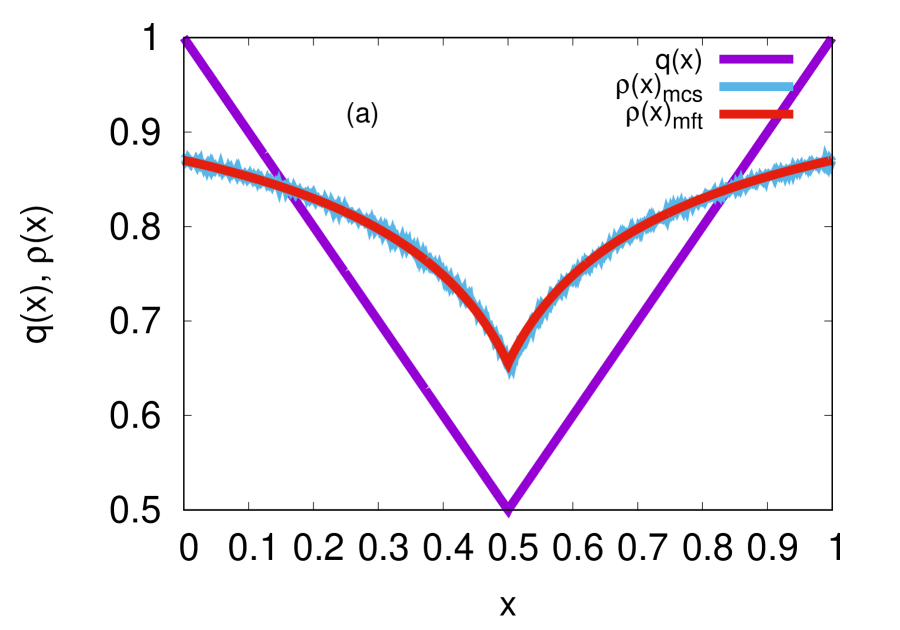
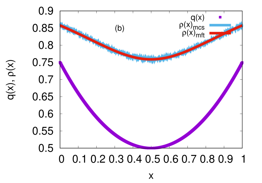
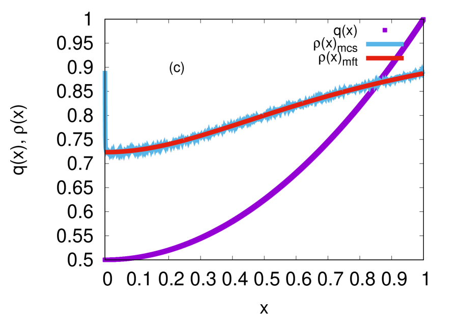
Figure 7: (a) Plot of $\rho(x)$ versus $x$ in the smooth phase for $q(x)=1-x,0\leq x<0.5;q(x)=x,0.5\leq x<1$ (purple continuous line), $n=0.8$. (b) Plot of $\rho(x)$ versus $x$ in the smooth phase for $q(x)=(x-0.5)^{2}+0.5$ (purple continuous line), $n=0.8$. (c) Plot of $\rho(x)$ versus $x$ in the smooth phase for $q(x)=0.5x^{2}+0.5$ (purple continuous line), $n=0.8$. Continuous magenta line and overlapping blue points represent, respectively, MFT and MCS data in each plot.

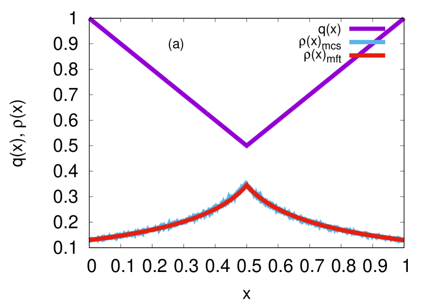
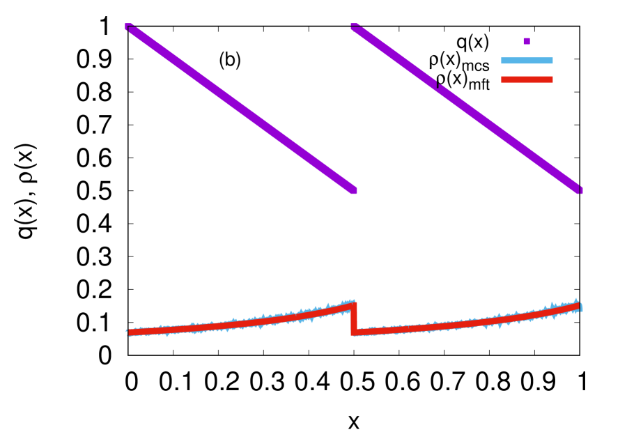
Figure 8: (a) Plot of $\rho(x)$ versus $x$ in the smooth phase for $q(x)=1-x,0\leq x<0.5;q(x)=x,0.5\leq x<1$ (purple continuous line), $n=0.2$. (b) Plot of $\rho(x)$ versus $x$ in the smooth phase for $q(x)=1-x,0\leq x<0.5;q(x)=1.5-x,0.5\leq x<1$ (purple), $n=0.1$ . Continuous magenta line and overlapping blue points represent, respectively, MFT and MCS data in each plot .

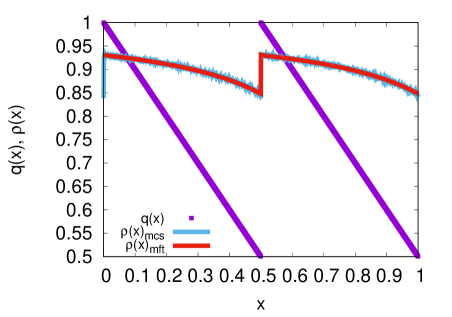
Figure 9: Plot of $\rho(x)$ versus $x$ in the smooth phase for $q(x)=1-x,0\leq x<0.5;q(x)=1.5-x,0.5\leq x<1$ (purple), $n=0.9$. Continuous magenta line and overlapping blue points represent, respectively, MFT and MCS data.

C.2 Density profiles in the shock phase

Here we present a few illustrative examples of the steady state density profiles in the shock phase; see Fig. 10.

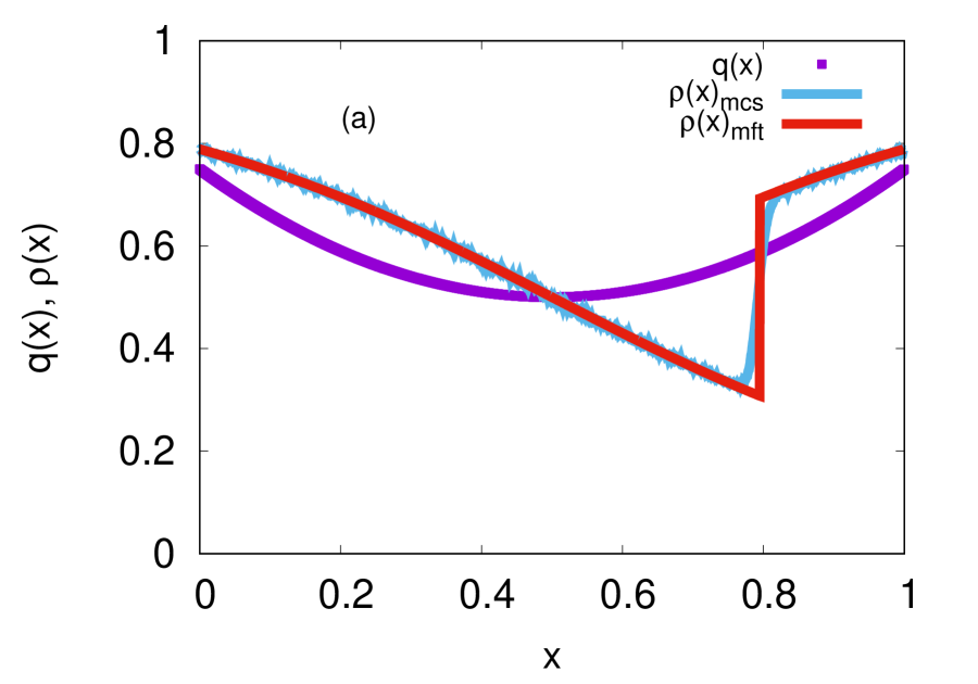
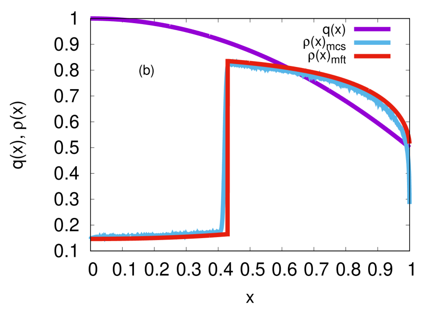
Figure 10: (a) Plot of $\rho(x)$ versus $x$ in the shock phase for $q(x)=(x-0.5)^{2}+0.5$ (purple continuous line), $n=0.6$. (b) Plot of $\rho(x)$ versus $x$ in the shock phase for $q(x)=1-0.5x^{2}$ (purple continuous line), $n=0.5$. Continuous magenta line and overlapping blue points represent, respectively, MFT and MCS data in each plot .

C.3 Density profile in the shock phase with four DDWs

Here we show results for the density profile when there are four DDWs, see Fig. 11.

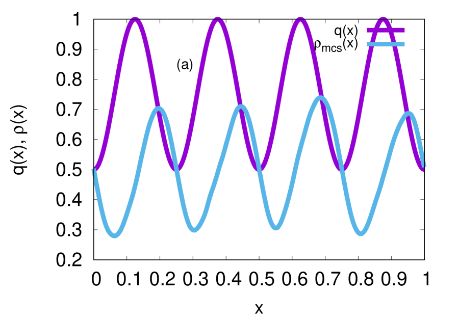
Figure 11: (a) MCS plot (blue dashed lines) of $\rho(x)$ versus $x$ for $q(x)=1-0.5\cos^{2}(4\pi x),n=0.5,N=1200$. The red solid lines and the blue dashed lines represent $q(x)$ and MCS data for $\rho(x)$ respectively. (b) Kymograph for $q(x)=1-0.5\cos^{2}(4\pi x),n=0.5,N=600$. Existence of four DDWs is clearly visible which move without any synchronization between any two of them.

References

- (1) J. Krug and P. A. Ferrari, J. Phys. A: Math. Gen. 29 L465 (1996); D. Chowdhury, L. Santen and A. Schadschneider, Phys. Rep. 329, 199 (2000); D. Helbing, Rev. Mod. Phys. 73, 1067 (2001).
- (2) C. Richer and S. Hasiak, Town Planning Review, Liverpool University Press, 2014, 85 (2), pp.217-236.
- (3) T. Karzig and F. von Oppen, Phys. Rev. B 81, 045317 (2010).
- (4) T Chou, K Mallick, and R K P Zia Rep. Prog. Phys. 74 116601 (2011).
- (5) S. E. Wells, E. Hillner, R. D. Vale and A. B. Sachs, Mol. Cell. 2, 135 (1998); S. Wang, K. S. Browning and W. A. Miller, EMBO J. 16, 4107 (1997).
- (6) Z. A. Afonina et al, Nucleic Acids Res. 42, 9461 (2014); D. W. Rogers et al, PLoS Comput. Biol. 13 e1005592 (2017).
- (7) L Jonathan Cook and R K P Zia J. Stat. Mech. P02012 (2009); L. Jonathan Cook, R. K. P. Zia, and B. Schmittmann, Phys. Rev. E 80, 031142 (2009).
- (8) T. Chou, Biophys. J 85, 755 (2003).
- (9) B. Derrida, E. Domany, D. Mukamel, J. Stat. Phys. 69, 667 (1992); B. Derrida, S. A. Janowsky, J. L. Lebowitz, E. R. Speer, J. Stat. Phys. 78, 813 (1993); B. Derrida, M.R. Evans, J. Physique I 3, 311 (1993).
- (10) J. Krug, Phys. Rev. Lett. 67, 1882 (1991).
- (11) R.K.P. Zia, J.J. Dong, and B. Schmittmann, J. Stat. Phys. 144, 405 (2011).
- (12) R. B. Stinchcombe and S. L. A. de Queiroz, Phys. Rev. E 83, 061113 (2011).
- (13) G. Tripathy and M. Barma, Phys. Rev. E 58, 1911 (1998).
- (14) M. Bengrine, A. Benyoussef, H. Ez-Zahraouy, and F. Mhirech, Phys. Lett. A 253, 135 (1999); C. Enaud and B. Derrida, Europhys. Lett. 66, 83 (2004).
- (15) L. B. Shaw, J. P. Sethna, and K. H. Lee, Phys. Rev. E 70, 021901 (2004).
- (16) A. Parmeggiani, T. Franosch, and E. Frey, Phys. Rev. Lett. 90, 086601 (2003).
- (17) J. Krug, Brazilian J. of Phys. 30, 97 (2000).
- (18) S. A. Janowsky and J. L. Lebowitz, Phys. Rev. A 45, 618 (1992).
- (19) N. Sarkar and A. Basu, Phys. Rev. E 90, 022109 (2014).
- (20) P. Pierobon, M. Mobilia, R. Kouyos and E. Frey, Phys. Rev. E 74, 031906 (2006).
- (21) T. Banerjee, N. Sarkar and A. Basu JStat. Mech.: Theory and Experiment P01024 (2015).
- (22) R. J. Harris and R. B. Stinchcombe, Phys. Rev. E 70, 016108 (2004).
- (23) B Alberts, A Johnson, J Lewis, M Raff, K Roberts, and P Walter, Molecular Biology of the Cell Garland Science, 4th edition (2002); B Li, M Carey, and J L Workman, Cell 128, 707 (2007); C Y Lin, J Lovén, P B Rahl, R M Paranal, C B Burge, J E Bradner, T I Lee, and R A Young, Cell 151, 56 (2012); J L Workman and R E Kingston, Annual Review of Biochemistry 67, 545 (1998).
- (24) D. D. Erdmann-Pham, K. D. Duc and Y. S. Song, arXiv: 1803.05609.
- (25) I. Buttinoni et al, J. Phys. Condens. Matter 24, 284129 (2012).
- (26) Q.-H. Wei, C. Bechinger, and P. Leiderer, Science 287, 625 (2000); C. Lutz, M. Kollmann, and C. Bechinger, Phys. Rev. Lett. 93, 026001 (2004).
- (27) C. Bechinger et al, Rev. Mod. Phys. 88, 045006 (2016).
- (28) T. Reichenbach, T. Franosch, and E. Frey, Eur. Phys. J E 27, 47 (2008).
- (29) U. Täuber, Critical Dynamics, Cambridge University Press (Cambridge, 2014).