Marked Length Spectrum, homoclinic orbits and the geometry of open dispersing billiards

Abstract.

We consider billiards obtained by removing three strictly convex obstacles satisfying the non-eclipse condition on the plane. The restriction of the dynamics to the set of non-escaping orbits is conjugated to a subshift on three symbols that provides a natural labeling of all periodic orbits. We study the following inverse problem: does the Marked Length Spectrum (i.e., the set of lengths of periodic orbits together with their labeling), determine the geometry of the billiard table? We show that from the Marked Length Spectrum it is possible to recover the curvature at periodic points of period two, as well as the Lyapunov exponent of each periodic orbit.

Introduction

In this paper, we study the spectral rigidity of a class of chaotic billiards obtained by removing $m\geq 3$ strictly convex obstacles from the plane ${\mathbb{R}}^{2}$. We assume that the boundary of each obstacle is at least of class $C^{3}$, and that the obstacles satisfy some non-eclipse condition. Similar billiard tables were already considered for instance in [GR], where the authors studied the classical scattering of a point particle from three hard circular discs in a plane. In [S], Stoyanov considered billiard trajectories in the exterior of two strictly convex domains in the plane, and obtained an asymptotic for the sequence of travelling times involving the distance between the two domains and the curvatures at the ends of the associated period two orbit. Yet, our perspective is dual to those works, in the sense that we focus on periodic orbits (in particular, such orbits do not escape to infinity), while in their case, they studied the deviation of escaping trajectories due to the presence of the obstacles.

By the strict convexity of the obstacles, the class of billiard tables we consider has some hyperbolic properties. Typically, hyperbolic systems have a lot of periodic orbits, in connection with the famous Anosov closing lemma, and it is thus natural to expect that the periodic data give a lot of information on the system. In this paper, we focus on the information given by the length of all periodic orbits. More precisely, by the chaoticity of the billiard and the non-eclipse condition we require, there is an embedded subshift of finite type which provides a natural labeling of the periodic orbits. Then, the Marked Length Spectrum is defined as the set of all lengths of periodic orbits together with their marking. The question we want to address is the following:

How much geometric information on the billiard table does the Marked Length Spectrum convey? In particular, are two such tables with the same Marked Length Spectrum necessarily isometric?

The problem of spectral rigidity. The problem of spectral rigidity has been investigated in various settings. Let us recall that it is connected with the famous problem of M. Kac [K]: “Can you hear the shape of a drum?”, i.e., whether the shape of a planar domain is determined by the Laplace Spectrum. For instance, Andersson-Melrose [AM], generalizing previous results, showed that for strictly convex $C^{\infty}$ domains, there exists a remarkable relation between the singular support of the wave trace and the Length Spectrum. In particular, the Laplace Spectrum determines the Length Spectrum in this setting. Similarly, there is a connection between Laplace Spectrum and Length Spectrum in hyperbolic situations. Indeed, the Selberg trace formula shows that the Laplace Spectrum determines the Length Spectrum on hyperbolic manifolds, and for generic Riemannian metrics, the Laplace Spectrum determines the Length Spectrum.

The Marked Length Spectrum determines a hyperbolic surface up to isometry. For hyperbolic surfaces, there is a natural marking of periodic trajectories by the homology, obtained as follows: to each homology class, we associate the length of the closed geodesic in this class. The question of spectral rigidity for hyperbolic surfaces was addressed by Otal [O] and independently by Croke [Cr]: they showed that if $g_{0}$ and $g_{1}$ are negatively curved metrics on a closed surface $S$ with the same Marked Length Spectrum, then $g_{1}$ is isometric to $g_{0}$ (see [CS] for the multidimensional case). More recently, Guillarmou-Lefeuvre [GL] proved that in all dimensions, the Marked Length Spectrum of a Riemannian manifold $(M,g)$ with Anosov geodesic flow and non-positive curvature locally determines the metric.

Spectral rigidity for (convex) real analytic domains with symmetries. Let us now mention a few results related to the question of spectral ridigity for convex billiards. It has been famously proven by Zelditch (see [Z1, Z2, Z3]) that the inverse spectral problem has a positive answer in the case of a generic class of real analytic ${\mathbb{Z}}_{2}$-symmetric plane convex domains (i.e., symmetric with respect to some reflection); in other terms, the Spectrum determines the geometry of such domains. Hezari-Zelditch [HZ2] have obtained a higher dimensional analogue of this result: bounded analytic domains ­in ${\mathbb{R}}^{n}$ with reflection symmetries across all coordinate axes, and with one axis height fixed (satisfying some generic non-degeneracy conditions) are spectrally determined among other such domains. Results of this kind are, currently, far beyond reach in the smooth category, although, in the last decade, interesting results have started to appear for the, weaker, spectral rigidity properties. In [HZ1], Hezari-Zelditch have shown the following result in the direction of the question of spectral ridigity: given a domain bounded by an ellipse, then any one-parameter isospectral $C^{\infty}$ deformation which additionally preserves the ${\mathbb{Z}}_{2}\times{\mathbb{Z}}_{2}$ symmetry group of the ellipse is necessarily flat (i.e., all derivatives have to vanish at the initial parameter).

On the other hand, Colin de Verdière has studied the dynamical version of the inverse spectral problem for billiards with symmetries: in [CdV], he has shown that in the case of convex analytic billiards which have the symmetries of an ellipse, the Marked Length Spectrum determines completely the geometry. In [DSKW], the authors have obtained the following result about the question of dynamical spectral rigidity: any sufficiently smooth ${\mathbb{Z}}_{2}$-symmetric strictly convex domain sufficiently close to a circle is dynamically spectrally rigid, i.e., all deformations among domains in the same class which preserve the length of all periodic orbits of the associated billiard flow must necessarily be isometries.

Lyapunov exponents of periodic orbits and the Marked Length Spectrum. In another direction, Huang-Kaloshin-Sorrentino [HKS] have proved that for a generic strictly convex domain, it is possible to recover the eigendata corresponding to Aubry-Mather periodic orbits of the induced billiard map, from the (maximal) Marked Length Spectrum of the domain. Here, the marking is defined by associating any rational number $r$ in $[0,\frac{1}{2}]$ with the maximum among all the perimeters of periodic orbits with rotation number $r$.

Flat billiards. Let us also mention that rigidity questions have also been explored in the context of flat billiards. In the recent paper [DELS], the authors define a Bounce Spectrum for polygons, recording the symbolic dynamics of the billiard flow, in the same way as the symbolic coding we introduce in the present paper. Then, they have shown that two simply connected Euclidean polygons with the same Bounce Spectrum are either similar or right-angled and affinely equivalent.

Dispersing billiards. A dual formulation of the inverse spectral problem is the inverse resonance problem, in which one attempts to reconstruct an unbounded domain (e.g. the complement of a finite number of convex scatterers) by the resonances (i.e. the poles) of the resolvent $(\Delta-z^{2})^{-1}$ (see e.g. [PS2, Zw, Z4]). From the dynamical point of view, these systems are described by the theory of Dispersing Billiards, which is today a very active topic in dynamical systems.

In this paper, we are exploring the inverse dynamical problem in this setting. We show that for the class of billiards introduced above, it is possible to reconstruct some geometric information from the Marked Length Spectrum, namely the radius of curvature at the bouncing points of period two orbits. Contrary to some of the results recalled above, we do not assume any additional symmetries. In fact, we use asymmetric orbits between the obstacles to recover separately the curvatures. In the same direction as in [HKS], we also show that for general periodic orbits, it is possible to adapt part of the procedure we introduce in the case of period two orbits in order to recover the Lyapunov exponent of each periodic orbit (see the paragraph before (3) for the definition of this notion). Yet, it seems that for general periodic orbits, we don’t have enough asymmetric information between the points in the orbit to distinguish between them on a differentiable level, and recover the curvature at each point separately. We continue the study of higher order periodic orbits in a separate work [BDSKL], where we discuss that by an argument of Livsic type, the information on Lyapunov exponents obtained here are sufficient to recover the differential of the billiard map, up to Hölder conjugacy, and we show that additional geometric quantities can be reconstructed from the Marked Length Spectrum. On the other hand, in [DSKL], we investigate the case of billiards of the same type as above, but with analytic boundary, and we show that if the billiard table has some symmetries, the square of the billiard map itself can be entirely reconstructed from the Marked Length Spectrum, as well as the geometry.

1. Preliminaries

1.1. Symbolic coding and Marked Length Spectrum

In this paper, we consider billiard tables $\mathcal{D}\subset{\mathbb{R}}^{2}$ given by $\mathcal{D}={\mathbb{R}}^{2}\setminus\bigcup^{3}_{i=1}\mathcal{O}_{i}$ where each $\mathcal{O}_{i}$ is a convex domain with boundary $\partial\mathcal{O}_{i}=\Gamma_{i}$, which we assume to be sufficiently smooth (of class at least $C^{3}$). We refer to each of the $\mathcal{O}_{i}$’s as obstacle or scatterer. We let $\ell_{i}:=|\Gamma_{i}|$ be the respective lengths, and we parametrize each $\Gamma_{i}$ in arc-length, for some smooth map $\gamma_{i}\colon{\mathbb{T}}_{i}:={\mathbb{R}}/\ell_{i}{\mathbb{Z}}\to{\mathbb{R}}^{2}$, $s\mapsto\gamma_{i}(s)$. We assume that the non-eclipse condition is satisfied, i.e., the convex hull of any two scatterers is disjoint from the third one.

We denote the collision space by

$$\mathcal{M} =\bigcup_{i}\mathcal{M}_{i}, \mathcal{M}_{i} =\{(q,v),\ q\in\Gamma_{i},\ v\in{\mathbb{R}}^{2},\ \|v\|=1,\ \langle v,n\rangle\geq 0\},$$

where $n$ is the unit normal vector to $\Gamma_{i}$ pointing inside $\mathcal{D}$. For each $x=(q,v)\in\mathcal{M}$, $q$ is associated with the arclength parameter $s\in[0,\ell_{i}]$ for some $i\in\{1,2,3\}$, i.e., $q=\gamma_{i}(s)$, and we let $\varphi\in[-\frac{\pi}{2},\frac{\pi}{2}]$ be the oriented angle between $n$ and $v$. In other terms, each $\mathcal{M}_{i}$ can be seen as a cylinder ${\mathbb{T}}_{i}\times[-\frac{\pi}{2},\frac{\pi}{2}]$ endowed with coordinates $(s,\varphi)$. In the following, given a point $x=(q,v)\in\mathcal{M}$ associated with the pair $(s,\varphi)$, we also denote by $\gamma(s):=q$ the point of the table defined as the projection of $x$ onto the $q$-coordinate. Set $\Omega:=\{(q,v)\in\mathcal{D}\times\mathbb{S}^{1}\}$. We denote by $\Phi^{t}\colon\Omega\to\Omega$ the flow of the billiard and let

$$\mathcal{F}\colon\mathcal{M}\to\mathcal{M},\quad x\mapsto\Phi^{\tau(x)+0}(x)$$

be the associated billiard map, where $\tau\colon\mathcal{M}\to{\mathbb{R}}_{+}\cup\{+\infty\}$ is the first return time. For each pair $(s,\varphi),(s^{\prime},\varphi^{\prime})\in\mathcal{M}$, we denote by

(1) $$h(s,s^{\prime}):=\|\gamma(s)-\gamma(s^{\prime})\|$$

the length of the segment connecting the associated points of the table.

By the convexity of the obstacles, for each $i\in\{1,2,3\}$, for $*\in\{j,k\}$, with $\{i,j,k\}=\{1,2,3\}$, there exist $0\leq a_{i}^{*}\leq b_{i}^{*}\leq\ell_{i}$, and for each parameter $s\in[a_{i}^{*},b_{i}^{*}]$, there exists a non-empty closed interval $I_{i}^{*}(s)\subset[-\frac{\pi}{2},\frac{\pi}{2}]$ such that $\tau(x)<+\infty$, if $x=(s,\varphi)\in\widetilde{\mathcal{M}}_{i}:=\widetilde{\mathcal{M}}_{i}^{j}\cup\widetilde{\mathcal{M}}_{i}^{k}$, and $\tau(x)=+\infty$, if $x\in\mathcal{M}_{i}\backslash\widetilde{\mathcal{M}}_{i}$, where

$$\widetilde{\mathcal{M}}_{i}^{*}:=\{(s,\varphi)\in\mathcal{M}_{i}:s\in[a_{i}^{*},b_{i}^{*}],\ \varphi\in I_{i}^{*}(s)\}=\mathcal{M}_{i}\cap\mathcal{F}^{-1}(\mathcal{M}_{*}).$$

In particular, the set of trajectories that do not escape to infinity is given by

$$\bigcap_{j\in{\mathbb{Z}}}\mathcal{F}^{-j}(\widetilde{\mathcal{M}}),\quad\widetilde{\mathcal{M}}:=\widetilde{\mathcal{M}}_{1}\cup\widetilde{\mathcal{M}}_{2}\cup\widetilde{\mathcal{M}}_{3},$$

and is homeomorphic to a Cantor set. In restriction to this set, the dynamics is conjugated to a subshift of finite type associated with the transition matrix

$$\begin{pmatrix}0&1&1\\ 1&0&1\\ 1&1&0\end{pmatrix}.$$

In other terms, any word $(\rho_{j})_{j}\in\{1,2,3\}^{\mathbb{Z}}$ such that $\rho_{j+1}\neq\rho_{j}$ for all $j\in{\mathbb{Z}}$ can be realized by an orbit, and by expansiveness of the dynamics, this orbit is unique. Such a word is called admissible. Besides, this marking is unique provided that we fix a starting point in the orbit and an orientation.

In particular, any periodic orbit of period $p\geq 2$ can be labelled by a finite admissible word $\sigma=(\sigma_{1}\sigma_{2}\dots\sigma_{p})\in\{1,2,3\}^{p}$, i.e., such that the infinite word $\sigma^{\infty}:=\dots\sigma\sigma\sigma\dots$ is admissible, or equivalently, such that $\sigma_{1}\neq\sigma_{p}$ and $\sigma_{j}\neq\sigma_{j+1}$, for all $j\in\{1,\dots,p-1\}$. We also let $\overline{\sigma}$ be the transposed word

$$\overline{\sigma}:=(\sigma_{p}\sigma_{p-1}\dots\sigma_{1}).$$

It still encodes the same periodic trajectory as $\sigma$, but traversed backwards.

As explained above, for any $j\in\{1,\dots,p\}$, the $j^{\text{th}}$ symbol $\sigma_{j}$ of $\sigma$ corresponds to a point $x(j)$ in the trajectory, where $x(j)=(s(j),\varphi(j))$ is represented by a position and an angle coordinates. For all $k\in{\mathbb{Z}}$, we also extend the previous notation by setting $\sigma_{k}:=\sigma_{\overline{k}}$, with $\overline{k}:=k\text{ (mod }p)$, and similarly for $x(k)$, $s(k)$ and $\varphi(k)$.

The Marked Length Spectrum of $\mathcal{D}$ is defined as the function

(2) $$\mathcal{L}\colon\sigma\mapsto\mathcal{L}(\sigma),\quad\sigma\in\cup_{p\geq 2}\{1,2,3\}^{p}\text{ finite admissible word},$$

where $\mathcal{L}(\sigma)$ is the length of the periodic orbit identified by $\sigma$, obtained by summing the lengths of all the line segments that compose it.

For any periodic orbit $(x_{1},\dots,x_{p})$ encoded by a word $\sigma$ of length $p\geq 2$, we have $D_{x_{j}}\mathcal{F}^{p}\in\mathrm{SL}(2,{\mathbb{R}})$, for $j\in\{1,\dots,p\}$. Due to the strict convexity of the obstacles, the matrix of the differential $D_{x_{j}}\mathcal{F}^{p}$ is hyperbolic, and we denote by $\mu(\sigma)>1$ (resp. $\lambda(\sigma):=\mu(\sigma)^{-1}<1$) its largest, (resp. smallest) eigenvalue. The Lyapunov exponent of this orbit is defined as $\mathrm{LE}(\sigma):=\frac{1}{p}\log\mu(\sigma)=-\frac{1}{p}\log\lambda(\sigma)>0$. Similarly, the Marked Lyapunov Spectrum of the billiard table $\mathcal{D}$ is defined as the function

(3) $$\mathrm{LE}\colon\sigma\mapsto\mathrm{LE}(\sigma),\quad\sigma\in\cup_{p\geq 2}\{1,2,3\}^{p}\text{ finite admissible word}.$$

1.2. Basic facts on chaotic billiards

Let us also recall a few useful facts about chaotic billiards; for more details, we refer to the book of Chernov-Markarian [CM].

We consider the billiard flow $\Phi^{t}\colon\Omega\to\Omega$. For any point $X=(q,v)\in\Omega$, we denote by $\omega\in[0,2\pi)$ the counterclockwise angle between the positive horizontal axis and the velocity vector $v$. The Jacobi coordinates $(d\eta,d\xi)$ in the subspace $T_{(x,y)}\mathcal{D}\subset T_{X}\Omega$ are defined as

$$d\eta=\cos\omega\,dx+\sin\omega\,dy,\qquad d\xi=-\sin\omega\,dx+\cos\omega\,dy.$$

In other terms, $d\eta$ is the component along the velocity vector $v$, and $d\xi$ is its orthogonal component. Let us introduce, furthermore, the subspace $T_{X}^{\perp}\Omega:=\{dX:\cos\omega\,dx+\sin\omega\,dy=0\}\subset T_{X}\Omega$ which is invariant for the flow in the sense that $D_{X}\Phi^{t}(T_{X}^{\perp}\Omega)=T_{\Phi^{t}X}^{\perp}\Omega$. The slope of a tangent line $L\subset T_{X}^{\perp}\Omega$ is defined as $\mathcal{B}:=\frac{d\omega}{d\xi}$. A smooth curve in $\mathcal{D}$ equipped with a continuous family of unit normal vectors is called a wave front; it is dispersing if it has positive slope, i.e., $\mathcal{B}>0$.

In the following, we restrict ourselves to the collision space $\mathcal{M}$, and we denote by $\|\cdot\|_{p}$ the $p$-metric on tangent vectors $(ds,d\varphi)$:

(4) $$\|(ds,d\varphi)\|_{p}:=\cos\varphi|ds|.$$

Loosely speaking, a smooth curve in the collision space is called a dispersing wave front if it is the projection on $\mathcal{M}$ of a dispersing wave front as above. More precisely, let $i\in\{1,2,3\}$, let $0<a<b<\ell_{i}$, and let $\mathcal{W}=\{(s,\phi(s)):a\leq s\leq b\}$, for some $C^{1}$ function $\phi\colon[a,b]\to[-\frac{\pi}{2},\frac{\pi}{2}]$. We define $\mathcal{B}^{+}$ as

$$\mathcal{B}^{+}(s):=\frac{\phi^{\prime}(s)+\mathcal{K}(s)}{\cos\phi(s)},\quad\forall\,a\leq s\leq b,$$

where $\mathcal{K}(s)$ is the curvature at the point with parameter $s$. Then, we say that $\mathcal{W}$ is a dispersing wave front if $\mathcal{B}^{+}(s)>0$, for all $a\leq s\leq b$. We denote its length by $|\mathcal{W}|:=\int_{\mathcal{W}}\|dx\|_{p}$. Then, for all $k\geq 0$, $\mathcal{F}^{k}(\mathcal{W})$ is a finite collection of dispersing wave fronts, and the sequence $(|\mathcal{F}^{k}(\mathcal{W})|)_{k\geq 0}$, which denotes the total length of these wave fronts, grows exponentially fast.

This follows from the following fact. Fix $x\in\mathcal{M}$, and let $x(k)=(s(k),\varphi(k))$, $k\geq 0$, be its forward iterates. Given any vector $dx=(ds,d\varphi)$ in the tangent line $L\subset T_{x}\mathcal{M}$, then for any $k\geq 0$, we have (see e.g. Chernov-Markarian [CM], p. 58)

(5) $$\frac{\|D_{x}\mathcal{F}^{k}\cdot dx\|_{p}}{\|dx\|_{p}}=\prod_{j=0}^{k-1}|1+\ell_{j}\mathcal{B}_{j}^{+}|,$$

where $\mathcal{B}_{j}^{+}$ denotes the slope of the postcolisional line $L_{j}^{+}$ corresponding to the line $L_{j}:=D_{x}\mathcal{F}^{j}(L)$ obtained after $j$ iterations, and $\ell_{j}:=h(s(j),s(j+1))$ denotes the length of the $j^{\text{th}}$ segment of the forward orbit of $x$ under $\mathcal{F}$. Moreover, $\mathcal{B}_{j+1}^{+}=\frac{\mathcal{B}_{j}^{+}}{1+\ell_{j}\mathcal{B}_{j}^{+}}+\frac{2\mathcal{K}(s_{j+1})}{\cos\varphi_{j+1}}$, which ensures that $\mathcal{B}_{j}^{+}>c$ for some $c>0$ that depends only on the billiard configuration.

To conclude, let us also recall some important symmetry of the billiard dynamics, which will be very useful in the following. Let us denote by $\mathcal{I}$ the map $\mathcal{I}\colon(s,\varphi)\mapsto(s,-\varphi)$. It conjugates the billiard map $\mathcal{F}$ with its inverse $\mathcal{F}^{-1}$, according to the time-reversal property of the billiard dynamics:

$$\mathcal{I}\circ\mathcal{F}\circ\mathcal{I}=\mathcal{F}^{-1}.$$

In the following, a periodic orbit of period $p=2q\geq 2$ is called palindromic if it can be labelled by an admissible word $\sigma\in\{1,2,3\}^{p}$ such that $\sigma=(\sigma_{1}\dots\sigma_{q-1}\sigma_{q}\sigma_{q-1}\dots\sigma_{1}\sigma_{0})$ for certain symbols $(\sigma_{0},\sigma_{1},\dots,\sigma_{q})\in\{1,2,3\}^{q+1}$. As we shall see later, there is a connection between the palindromic symmetry and the time-reversal property recalled above. In particular, by the palindromic symmetry and by expansiveness of the dynamics, the associated trajectory hits the billiard table perpendicularly at the points with symbols $\sigma_{0}$ and $\sigma_{q}$.

2. Statement of the results

2.1. The case of period two orbits

In this part, we consider billiard tables $\mathcal{D}\subset{\mathbb{R}}^{2}$ as above, and we focus on periodic orbits of period two. There are three such orbits, realized as the minimizing segments between each pair of obstacles.

Theorem A.

Consider a period two orbit encoded by a word $\sigma=(\sigma_{1}\sigma_{0})\in\{1,2,3\}^{2},\sigma_{0}\neq\sigma_{1}$. Let $\tau_{1}$ be such that $\{\tau_{1},\sigma_{0},\sigma_{1}\}=\{1,2,3\}$, and set $\tau:=(\tau_{1}\sigma_{0})$. We denote by $R_{0},R_{1}>0$ the respective radii of curvature at the points with symbols $\sigma_{0},\sigma_{1}$, and let $\lambda=\lambda(\sigma)<1$ be the smallest eigenvalue of $D\mathcal{F}^{2}$ at the points of $\sigma$.

Then, for $n\gg 1$, the following estimates hold:

1. if $n$ is even, then

   $$\mathcal{L}(\tau\sigma^{n})-(n+1)\mathcal{L}(\sigma)-\mathcal{L}^{\infty}=-C\cdot\mathcal{Q}\left(\frac{2R_{0}}{\mathcal{L}(\sigma)},\frac{2R_{1}}{\mathcal{L}(\sigma)}\right)\lambda^{n}+O(\lambda^{\frac{3n}{2}});$$

2. if $n$ is odd, then

   $$\mathcal{L}(\tau\sigma^{n})-(n+1)\mathcal{L}(\sigma)-\mathcal{L}^{\infty}=-C\cdot\mathcal{Q}\left(\frac{2R_{1}}{\mathcal{L}(\sigma)},\frac{2R_{0}}{\mathcal{L}(\sigma)}\right)\lambda^{n}+O(\lambda^{\frac{3n}{2}}),$$

for some real number $\mathcal{L}^{\infty}=\mathcal{L}^{\infty}(\sigma,\tau)\in{\mathbb{R}}$, some constant $C=C(\sigma,\tau)>0$, and a quadratic form $\mathcal{Q}\colon{\mathbb{R}}\times{\mathbb{R}}\to{\mathbb{R}}$ of the form

$$\mathcal{Q}(X,Y):=(1+\lambda^{2})(1+X)^{2}-(1+\lambda)^{2}XY+2\lambda(1+Y)^{2}.$$

Finally, the eigenvalue $\lambda<1$ is solution to the equation

$$4\lambda\left(\frac{\mathcal{L}(\sigma)}{2R_{0}}+1\right)\left(\frac{\mathcal{L}(\sigma)}{2R_{1}}+1\right)=(1+\lambda)^{2}.$$

Corollary B.

With the same notation as in Theorem A, we have

$$\mathrm{LE}(\sigma) =\frac{1}{2}\log(\mu)=-\frac{1}{2}\log(\lambda)=-\lim_{n\to+\infty}\frac{1}{2n}\log\left(-\mathcal{L}(\tau\sigma^{n})+(n+1)\mathcal{L}(\sigma)+\mathcal{L}^{\infty}\right).$$

In particular, the value of the Lyapunov exponent of $\sigma=(\sigma_{1}\sigma_{0})$ is determined by the Marked Length Spectrum.

Remark 2.1.

In the case of two strictly convex obstacles, Stoyanov [S] considered expressions similar to those in Theorem A but for sequences of travelling times of billiard trajectories with $n\geq 1$ reflection points between the two scatterers instead of lengths of periodic orbits (there is a unique periodic orbit in this situation, of period two), and showed an analogous asymptotic with an exponentially small error term. Based on that, he was able to recover the distance between the two obstacles and the Lyapunov exponent of the unique period two orbit. For further related results see also Section 10.3 in [PS1] and Section 7 in [PS2].

The proof of Theorem A is given in Section 5.3, and is based on a procedure explained in Section 3, where we introduce a sequence of periodic orbits shadowing some orbit that is homoclinic to the period two orbit $\sigma$. Such orbits capture local geometric information on the orbit $\sigma$. First, we estimate the parameters of the points in these orbits, and then we show that when we combine the lengths of these orbits in an appropriate way, then the differences converge to zero exponentially fast, at the rate given by the Lyapunov exponent of $\sigma$. Besides, the error term is maximal near the orbit $\sigma$, which allows us to extract some geometric information on $\sigma$.

Recall that the curvature $\mathcal{K}$ at a point of the table is defined as the inverse of the radius of curvature $R$, i.e., $\mathcal{K}=R^{-1}$. Then, Theorem A has the following geometric consequence (see Corollary 5.8 in Subsection 5.4 and also Corollary 5.9 where we derive other spectral invariants).

Corollary C.

The curvatures $\mathcal{K}_{0}$ and $\mathcal{K}_{1}$ at the bouncing points of periodic orbits of period two are determined by the Marked Length Spectrum (hence also the value of the constant $C$ in Theorem A).

Actually, we have $\lim_{n\to+\infty}\mathrm{LE}(\tau\sigma^{n})=\mathrm{LE}(\sigma)$, and by considering Taylor expansions of $\mathrm{LE}(\tau\sigma^{n})$, we have also shown that it is possible to recover the respective derivatives of the curvature $\mathcal{K}_{0}^{\prime}$ and $\mathcal{K}_{1}^{\prime}$ at the two bouncing points of the orbit $\sigma$.

As an illustration of the above results, we show that the geometry of certain billiard tables is entirely determined by the Marked Length Spectrum.

Remark 2.2 (See Corollary 5.7 and the proof that follows).

The Marked Length Spectrum determines completely the geometry of billiard tables $\mathcal{D}={\mathbb{R}}^{2}\setminus\{\mathcal{O}_{1},\mathcal{O}_{2},\dots,\mathcal{O}_{m}\}$ obtained by removing from the plane $m\geq 3$ round discs $\mathcal{O}_{1},\dots,\mathcal{O}_{m}$ which satisfy the non-eclipse condition, i.e., such that the convex hull of any two obstacles is disjoint from the other obstacles.

2.2. Marked Length Spectrum and Marked Lyapunov Spectrum

We consider a periodic orbit of period $p\geq 2$, encoded by some admissible word $\sigma=(\sigma_{1}\sigma_{2}\dots\sigma_{p})\in\{1,2,3\}^{p}$. We denote by $\lambda=\lambda(\sigma)<1$ the smallest eigenvalue of $D\mathcal{F}^{p}$ at the points in the orbit.

Let $\tau=(\tau^{-},\tau^{+})\in\{1,2,3\}^{2}$ be such that $\tau^{-}\neq\sigma_{p}$ and $\tau^{+}\neq\sigma_{1}$. For any integer $n\geq 0$, we define the two words

$$h_{n}^{+}(\sigma,\tau) :=(\tau^{+}\sigma^{n}\tau^{-}\overline{\sigma}^{n}):=(\tau^{+}\underbrace{\sigma\sigma\dots\sigma}_{\text{n\ \text{times}}}\tau^{-}\underbrace{\overline{\sigma\sigma\dots\sigma}}_{\text{n\ \text{times}}}),$$

$$h_{n}^{-}(\sigma,\tau) :=(\tau^{-}\overline{\sigma}^{n}\tau^{+}\sigma^{n}):=(\tau^{-}\underbrace{\overline{\sigma\sigma\dots\sigma}}_{\text{n\ \text{times}}}\tau^{+}\underbrace{\sigma\sigma\dots\sigma}_{\text{n\ \text{times}}}).$$

Note that the symbolic representations are just shifted by $np+1$ symbols, hence $h_{n}^{+}(\sigma,\tau)$ and $h_{n}^{-}(\sigma,\tau)$ correspond to the same periodic orbit of period $2np+2$, denoted by $h_{n}^{\prime}$ in the following. Also, this orbit $h_{n}^{\prime}$ is palindromic, which implies that the bounces at the symbols $\tau^{+}$ and $\tau^{-}$ are perpendicular.

Theorem D.

There exist a real number $\mathcal{L}^{\infty}(\sigma,\tau)\in{\mathbb{R}}$ and two constants $C_{\mathrm{even}}(\sigma,\tau),C_{\mathrm{odd}}(\sigma,\tau)>0$ such that for $n\gg 1$,

1. if $n$ is even, then

   $$\mathcal{L}(h_{n}^{\prime}(\sigma,\tau))-2n\mathcal{L}(\sigma)-\mathcal{L}^{\infty}(\sigma,\tau)=-C_{\mathrm{even}}(\sigma,\tau)\cdot\lambda^{n}+O(\lambda^{\frac{3n}{2}});$$

2. if $n$ is odd, then

   $$\mathcal{L}(h_{n}^{\prime}(\sigma,\tau))-2n\mathcal{L}(\sigma)-\mathcal{L}^{\infty}(\sigma,\tau)=-C_{\mathrm{odd}}(\sigma,\tau)\cdot\lambda^{n}+O(\lambda^{\frac{3n}{2}}).$$

The proof of the above theorem is given in Section 6 and is along the same lines as in the case of the period two. As a direct consequence of Theorem D, we obtain:

Corollary E.

The Marked Lyapunov Spectrum is entirely determined by the Marked Length Spectrum (see (2) and (3) for the definitions).

Theorem D for arbitrary period $p\geq 3$ is weaker than Theorem A for period two, because of two reasons. First, observe that period two orbits are in a sense degenerate, namely, their local dynamics has only two free parameters. Indeed, the length of each side is given by the Marked Length Spectrum, the angles of reflections are $\frac{\pi}{2}$, and the only free parameters are the two curvatures at the two collision points. Meanwhile, period $p\geq 3$ orbits have $3p-2$ parameters: $p-1$ independent orbit segments’ lengths, $p-1$ independent angular data and $p$ curvatures at bouncing points. More precisely, to prove an analog of Theorem A we face the following problem.

Remark 2.3.

The proofs of Theorem A in the period two case and Theorem D for a general periodic orbit $\sigma$ are based on precise estimates on the parameters of certain sequences of orbits which approximate $\sigma$. Such estimates are obtained by linearizing the dynamics; indeed, each point in the orbit $\sigma$ is a saddle fixed point of the $p^{\text{th}}$ iterate of the billiard map $\mathcal{F}$, where $p\geq 2$ is the period of $\sigma$. This yields two independent relations according to the parity of the number $n\geq 0$ of repetitions of $\sigma$ in the coding of the approximating sequences. Besides, those relations carry some asymmetric information between the points of $\sigma$. This is enough to reconstruct the curvature for period two orbits (Corollary C), but it is insufficient when the period $p$ is at least $3$, due to the large number of parameters encoded implicitly by $\mathcal{F}^{p}$. One (unsuccessful) strategy that we have tried to produce more relations was to shift the reference point of $\sigma$ and vary the word $\tau$ used to define approximating sequences. This does modify the geometry of the associated orbits; yet, those changes happen “far” from the orbit $\sigma$ that we want to describe, while the estimates in Theorem D are obtained by considering points in a neighborhood of $\sigma$. Such changes result in a scaling of the asymptotic constants in the estimates of Subsection 6.1, but do not give any additional asymmetric information to distinguish between the points of $\sigma$.

Organization of the paper

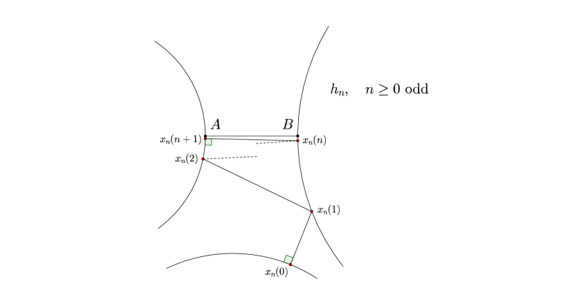
Figure 1. Approximation of the homoclinic orbit to the period two orbit between the first two obstacles (here we assume that $n$ is odd).

The rest of the paper is organized as follows. We fix a period two orbit $AB$ (see Fig. 1). In Section 3 and Section 4 we describe a class of homoclinic orbits to $AB$ and estimate the speed these homoclinic orbits are approximated by periodic orbits. In Section 5 we utilize these estimates, prove Theorem A, and derive the associated constants. In Section 6, we prove Theorem D and its Corollaries.

3. Estimates on periodic orbits shadowing some homoclinic orbit

3.1. Idea of the construction

In the following, we explain a geometric construction which allows us to extract from the Marked Length Spectrum some geometric information near a periodic orbit. In most of the paper, we explain in detail this procedure in the case where the periodic orbit has period two. As we shall see later, the general construction as well as most estimates remain true for more general periodic orbits. Yet, period two orbits have special features which make them nicer to deal with, namely:

• they have some palindromic symmetry; loosely speaking, this will be especially useful in the following in order to connect the future and the past of certain orbits that we introduce in the construction;

• we know the angles at the two bouncing points (the orbit hits the table perpendicularly at these two points) as well as the length of the two arcs of the orbit (they are equal to half of the total length of the orbit). In particular, if we want to describe the local geometry near the points of the orbit, then at the leading order, the only quantity to reconstruct is the radius of curvature at the two bouncing points.

The construction we are about to describe is based on an orbit homoclinic to the chosen period two orbit identified by $\sigma$, which conveys a lot of geometric information on $\sigma$ (the same homoclinic orbit was considered in the aforementioned work of Stoyanov [S]). However since this orbit is not periodic, this information is not readily available in the Marked Length Spectrum. Therefore, we define a sequence $(h_{n})_{n\geq 0}$ of periodic orbits which shadow more and more closely this homoclinic orbit. Exploiting the symbolic coding of the dynamics, such orbits are obtained by truncating the infinite word associated to the homoclinic orbit in order to produce a finite word, which then corresponds to a periodic orbit (see Figure 1). By expansivity of the dynamics, the the sequence $(h_{n})_{n\geq 0}$ converges to the limit homoclinic orbit exponentially fast, whose rate is related to the Lyapunov exponent of the period two orbit (which is also the Lyapunov exponent of the homoclinic orbit). By comparing the length of $h_{n}$ with the length of the original period two orbit, we see that the estimates involve two different constants depending on the parity of $n\geq 0$. This is due to some asymmetry in the orbits $h_{n}$: indeed, as we will see, among all the points in the orbits $h_{n}$, there is exactly one bounce which is closest to the period two orbit that we approximate, and this bounce is on one of the two obstacles associated to the period two orbit, which depends on the parity of $n$. Combining these estimates with the properties of period two orbits that we described above, we see that this is actually sufficient to recover the radius of curvature at each point of the period two orbit under construction.

3.2. The case of period two orbits

In this part, we focus on the first two obstacles $\mathcal{O}_{1},\mathcal{O}_{2}$, and on the period two orbit between them. It is labelled by the word $\sigma=(12)$ according to the marking introduced earlier. We denote by $\mathcal{L}(12)$ the length of the periodic orbit $(12)$, and we denote by $A$ (resp. $B$), the point in the orbit which lies on the boundary $\Gamma_{1}$ of the first obstacle (resp. on the boundary $\Gamma_{2}$ of the second obstacle). We let $\ell:=\frac{1}{2}\mathcal{L}(12)$ be the distance between the points $A$ and $B$ in the plane, and we assume that $A=(-\frac{1}{2}\ell,0)$ and $B=(\frac{1}{2}\ell,0)$. We also choose the parametrizations of $\mathcal{M}_{i}$, $i\in\{1,2,3\}$, in such a way that $(0,0)=(0_{1},0)$ (resp. $(0,0)=(0_{2},0)$), are the $(s,\varphi)$-coordinates of the (perpendicular) bounce of the orbit $\sigma$ at the point $A$ (resp. $B$). In particular, we have $A=\gamma_{1}(0)$ and $B=\gamma_{2}(0)$.

For $\{i,j\}=\{1,2\}$, the matrix of the differential of the billiard map $\mathcal{F}$ in $(s,\varphi)$-coordinates at the point with coordinates $(0_{i},0)$ is

$$D_{(0_{i},0)}\mathcal{F}=-\begin{pmatrix}\frac{\ell}{R_{i}}+1&\ell\\ \frac{\ell}{R_{i}R_{j}}+\frac{1}{R_{i}}+\frac{1}{R_{j}}&\frac{\ell}{R_{j}}+1\end{pmatrix},$$

where $R_{1}=\mathcal{K}_{1}^{-1}$ (resp. $R_{2}=\mathcal{K}_{2}^{-1}$) denotes the radius of curvature at the point $A$ (resp. $B$).

The periodic orbit $(12)$ is hyperbolic. We denote by $\lambda=\lambda(12)<1$, $\mu=\mu(12):=\lambda^{-1}>1$ the common eigenvalues of the differentials $D_{(0_{1},0)}\mathcal{F}^{2}=D_{(0_{2},0)}\mathcal{F}\circ D_{(0_{1},0)}\mathcal{F}$ and $D_{(0_{2},0)}\mathcal{F}^{2}=D_{(0_{1},0)}\mathcal{F}\circ D_{(0_{2},0)}\mathcal{F}$. In particular, $\pm\frac{1}{2}\log\mu=\mp\frac{1}{2}\log\lambda$ are the two Lyapunov exponents of the hyperbolic fixed points $(0_{1},0)$ and $(0_{2},0)$ of $\mathcal{F}^{2}$.

Lemma 3.1.

For any $x=(s,\varphi)\in\widetilde{\mathcal{M}}$, the point $\gamma(s)\in\partial\mathcal{D}\subset{\mathbb{R}}^{2}$ is in the region of the plane bounded by the three segments and the three arcs connecting the points in period two orbits.

Proof.

Let us assume, by contradiction, that there exists some $x_{0}=(s_{0},\varphi_{0})\in\widetilde{\mathcal{M}}$ such that the associated point in $\partial\mathcal{D}$ lies on $\Gamma_{1}$ beyond the point $A$, i.e., such that $\gamma_{1}(s_{0})=(\bar{x},\bar{y})$, with $\bar{y}>0$. After possibly replacing $x_{0}$ with $\mathcal{I}(x_{0})=(s_{0},-\varphi_{0})$, we may assume that $\varphi_{0}\geq 0$, in such a way that the associated vector does not point towards the segment AB. Indeed, by the time-reversal property, the orbit of $\mathcal{I}(x_{0})$ under $\mathcal{F}$ is the orbit of $x_{0}$ traversed backwards, hence this change does not affect the fact that the orbit escapes to infinity or not. Let us denote by $(x(n)=(s(n),\varphi(n)))_{n\geq 0}$, the forward iterates of $x(0):=x_{0}$ under $\mathcal{F}$. By strict convexity of the obstacles, the sequences $(\varphi(2k))_{k\geq 0}$ and $(-\varphi(2k+1))_{k\geq 0}$ are strictly increasing, and then, the associated points in $\partial\mathcal{D}$ never come back to the region below the segment $AB$. Therefore, the symbolic coding of the forward orbit $(x(n))_{n\geq 0}$ is $121212\dots$, which is also the coding of the forward iterates of the point $(0_{1},0)$ in the period two orbit $(12)$. By the exponential growth of wave fronts (see (5)), this implies that $x_{0}$ is in the stable manifold of the point $(0_{1},0)$. Therefore, $\lim_{k\to+\infty}x(2k)=(0_{1},0)$, and the sequence $(\varphi(2k))_{k\geq 0}$ converges to $0$, a contradiction, since it is also non-negative and strictly increasing.

Let us give a few more details. Take a continuous monotonic map $\phi\colon[0,s_{0}]\to{\mathbb{R}}_{+}$ such that $\phi(0)=0$ and $\phi(s_{0})=\varphi_{0}$, and set

$$\mathcal{W}^{(2k)}:=\{x^{(2k)}(s):=\mathcal{F}^{2k}(s,\phi(s)):0\leq s\leq s_{0}\},\quad\forall\,k\geq 0.$$

By the strict convexity of the obstacles, and since the symbolic coding of $(x(n))_{n\geq 0}$ is $121212\dots$, then for each $k\geq 0$, $\mathcal{W}^{(2k)}$ is a dispersing wave front whose projection on the table is the arc of $\Gamma_{1}$ bounded by the points $A$ and $\gamma_{1}(s(2k))$. We obtain

$$|\mathcal{W}^{(2k)}|=\left|\int_{0}^{s_{0}}\|D_{x^{(0)}(s)}\mathcal{F}^{2k}\cdot(x^{(0)})^{\prime}(s)\|_{p}\,ds\right|$$

$$\geq\Lambda^{(2k)}\left|\int_{0}^{s_{0}}\|(x^{(0)})^{\prime}(s)\|_{p}\,ds\right|\geq\Lambda^{(2k)}\cdot\|x^{(0)}(s_{0})\|_{p}=\Lambda^{(2k)}\cdot\|x_{0}\|_{p}.$$

By (5), the sequence $(\Lambda^{(2k)})_{k\geq 0}$ goes to $+\infty$, while the left hand side is uniformly bounded. Letting $k\to+\infty$, we deduce that $x_{0}=(s_{0},\varphi_{0})=(0_{1},0)$, and thus $\gamma_{1}(s_{0})=\gamma_{1}(0_{1})=A$, a contradiction. ∎

3.3. Shadowing by palindromic periodic orbits

For any integer $n\geq 0$, we introduce the periodic orbit $h_{n}$ associated to the symbolic coding

$$h_{n}:=(32|(12)^{n})=(32\underbrace{121212\dots 1212}_{\text{2n}}).$$

The period of the orbit $h_{n}$ is equal to $2n+2$. We denote by $x_{n}(k)=(s_{n}(k),\varphi_{n}(k))_{k=0,\dots,2n+1}$ the $(s,\varphi)$-coordinates of the points in this orbit, and we extend them to all integer indices by setting $x_{n}(k):=x_{n}(k\text{ mod }(2n+2))$, for all $k\in{\mathbb{Z}}$. We label the points of $h_{n}$ in such a way that one period of this orbit matches the following geometric description:

• there is a unique perpendicular bounce on the third obstacle, with coordinates $(s_{n}(0),0)$;

• the following $n$ bounces alternate between the first and the second obstacle, getting closer to the periodic orbit $(12)$ each time; for each integer $k\in\{1,\dots,n\}$, the point with coordinates $(s_{n}(k),\varphi_{n}(k))$ is associated to a point on the first obstacle, resp. the second obstacle, whenever the index $k$ is even, resp. odd; in particular, the second bounce $(s_{n}(1),\varphi_{n}(1))$ is always on the second obstacle;

• the next point has coordinates $(s_{n}(n+1),0)$ and is associated to a perpendicular bounce on the first obstacle, resp. second obstacle, whenever $n$ is odd, resp. even; it is the point of $h_{n}$ which is closest to the orbit $(12)$;

• the next $n$ bounces correspond to the same points as for $k\in\{1,\dots,n\}$, the new orbit segment being the previous one traversed backwards.
  

We see that the orbit $h_{n}$ is asymmetric between the obstacles $1$ and $2$, in the sense that for each odd integer $n\geq 0$, the point of $h_{n}$ which is closest to the period two orbit $(12)$ is on the first obstacle, while for each even integer $n\geq 0$, the point of $h_{n}$ which is closest to the period two orbit $(12)$ is on the second obstacle.

The last item of the above description follows from the following result.

Lemma 3.2.

For any $k\in\{0,\dots,n+1\}$, we have

$$s_{n}(2n+2-k)=s_{n}(k),\qquad\varphi_{n}(2n+2-k)=-\varphi_{n}(k).$$

This explains why each of the orbit segments associated to indices in $\{n+1,\dots,2n+2\}$ is one of the orbit segments associated to indices in $\{0,\dots,n+1\}$, traversed backwards, according to the above description. In particular, this also implies that $\varphi_{n}(0)=\varphi_{n}(n+1)=0$.

Proof.

The proof follows from some palindromic property of the orbits $h_{n}$, $n\geq 0$. Indeed, for any even integer $n\geq 0$, we have

$$\dots|h_{n}|h_{n}|\ldots=\dots|\underset{\begin{subarray}{c}\uparrow\end{subarray}}{3}21212\dots 1\underset{\begin{subarray}{c}\uparrow\end{subarray}}{2}1\dots 21212|\underset{\begin{subarray}{c}\uparrow\end{subarray}}{3}21212\dots 1\underset{\begin{subarray}{c}\uparrow\end{subarray}}{2}1\dots 21212|\dots$$

and for any odd integer $n\geq 0$, we have

$$\dots|h_{n}|h_{n}|\ldots=\dots|\underset{\begin{subarray}{c}\uparrow\end{subarray}}{3}21212\dots 2\underset{\begin{subarray}{c}\uparrow\end{subarray}}{1}2\dots 21212|\underset{\begin{subarray}{c}\uparrow\end{subarray}}{3}21212\dots 2\underset{\begin{subarray}{c}\uparrow\end{subarray}}{1}2\dots 21212|\dots$$

We see that the above symbolic expansions are palindromic at the points marked with arrows, i.e., the future and the past of such points have the same symbolic coding.

Recall that the map $\mathcal{I}\colon(s,\varphi)\mapsto(s,-\varphi)$ switches future and past, according to the time-reversal property $\mathcal{I}\circ\mathcal{F}\circ\mathcal{I}=\mathcal{F}^{-1}$ of the billiard dynamics. Let us consider the point $x_{n}(n+1)$. Due to the palindromic symmetry, the orbits of $x_{n}(n+1)$ and $\mathcal{I}(x_{n}(n+1))$ under $\mathcal{F}$ have the same symbolic coding. By expansivity of the dynamics of $\mathcal{F}$, we conclude that $\mathcal{I}(x_{n}(n+1))=x_{n}(n+1)$, and thus, $\varphi_{n}(n+1)=0$. For the same reason, we have $\varphi_{n}(0)=0$. Then, for any $k\in\{0,\dots,n+1\}$, we obtain

$$(s_{n}(2n+2-k),-\varphi(2n+2-k)) =\mathcal{I}\circ\mathcal{F}^{n+1-k}(x_{n}(n+1))$$

$$=\mathcal{F}^{k-n-1}\circ\mathcal{I}(s_{n}(n+1),0)$$

$$=\mathcal{F}^{k-n-1}(x_{n}(n+1))$$

$$=(s_{n}(k),\varphi_{n}(k)).\qed$$

3.4. Preliminary estimates on the parameters at bounces

Lemma 3.3.

There exists a constant $\Lambda>1$ such that for any integers $n,p\geq 0$, and for any integer $k\in\{0,\dots,2n+1\}$, we have

(6) $$\|x_{n}(k)-x_{n+p}(k)\|=O(\Lambda^{-(2n+1)+k}).$$

Proof.

Let $n,p\geq 0$. Recall that $x_{n}(0)=(s_{n}(0),0)$ and that $x_{n+p}(0)=(s_{n+p}(0),0)$. In particular, the piece of $\Gamma_{3}=\partial\mathcal{O}_{3}$ lying between the above points endowed with $0$ angle in all points is a dispersing wave front, that we denote by $\mathcal{W}_{n,p}(0)\subset\mathcal{M}$. For all $0\leq k\leq 2n+1$, we set $\mathcal{W}_{n,p}(k):=\mathcal{F}^{k}(\mathcal{W}_{n,p}(0))$; it is also a dispersing wave front. The forward orbits of $x_{n}(0)$ and $x_{n+p}(0)$ have the respective symbolic codings

$$3\underbrace{21212\dots 21212}_{2n+1}|3\dots,\qquad 3\underbrace{21212\dots 21212}_{2n+1}|1\dots,$$

hence the projection of $\mathcal{W}_{n,p}(k)$ on the billard table is an arc of $\Gamma_{1}$, resp. $\Gamma_{2}$, when $0\leq k\leq 2n+1$ is even, resp. odd. Recall that $\|\cdot\|_{p}$ is the $p$-metric on tangent vectors in $T\mathcal{M}$ as in (4), and that for all $0\leq k\leq 2n+1$, we denote by $|\mathcal{W}_{n,p}(k)|:=\int_{\mathcal{W}_{n,p}(k)}\|dx\|_{p}$ the length of the associated wave front.

Take $x=(t,0)\in\mathcal{W}_{n,p}(0)$, and denote by $x(t,k)=(s(t,k),\varphi(t,k))\in\mathcal{W}_{n,p}(k)$, $0\leq k\leq 2n+1$, its forward iterates. Given any vector $dx=(ds,d\varphi)$ in the tangent line $L\subset T_{x}\mathcal{M}$, then as in (5), for all $0\leq k\leq 2n+1$, we have

$$\frac{\|D_{x}\mathcal{F}^{k}\cdot dx\|_{p}}{\|dx\|_{p}}=\prod_{j=0}^{k-1}|1+\ell_{j}\mathcal{B}_{j}^{+}|,$$

with $\ell_{j}:=h(s(t,j),s(t,j+1))$. In our case, Lemma 3.1 ensures that $\ell_{j}\geq\ell_{\text{min}}$ and $\mathcal{B}_{j}^{+}\geq\mathcal{B}_{\text{min}}$ for some constants $\ell_{\text{min}},\mathcal{B}_{\text{min}}>0$ which are uniform in $n\geq 0$, and thus,

$$\frac{\|D_{x}\mathcal{F}^{k}\cdot dx\|_{p}}{\|dx\|_{p}}\geq\Lambda^{k},$$

with $\Lambda:=1+\ell_{\text{min}}\mathcal{B}_{\text{min}}>1$. Therefore, for any $0\leq k\leq 2n+1$, the size $|\mathcal{W}_{n,p}(k)|$ of the image by $\mathcal{F}^{k}$ of the initial wave front $|\mathcal{W}_{n,p}(0)|$ satisfies

$$|\mathcal{W}_{n,p}(k)| =\int_{\mathcal{W}_{n,p}(0)}\|D_{x}\mathcal{F}^{k}\cdot dx\|_{p}=\left|\int_{s_{n}(0)}^{s_{n+p}(0)}\big{\|}D_{(t,0)}\mathcal{F}^{k}\cdot\frac{d}{dt}(t,0)\big{\|}_{p}\,dt\right|$$

$$\geq\Lambda^{k}\left|\int_{s_{n}(0)}^{s_{n+p}(0)}\|(1,0)\|_{p}\,ds\right|=\Lambda^{k}|s_{n+p}(0)-s_{n}(0)|.$$

As we have seen, for all $0\leq k\leq 2n+1$, the projection of $\mathcal{W}_{n,p}(k)$ is an arc of $\Gamma_{1}$ or $\Gamma_{2}$, hence $|\mathcal{W}_{n,p}(k)|\leq C$, for some constant $C>0$ depending only on the geometry of the table. We thus obtain

$$|s_{n+p}(0)-s_{n}(0)|\leq C\Lambda^{-(2n+1)}.$$

By Lemma 3.1 and the non-eclipse condition, for all $x\in\mathcal{W}_{n,p}(0)$, and $0\leq k\leq 2n+1$, the cosine of the angle of reflection of $\mathcal{F}^{k}(x)$ is lower bounded by some uniform constant $c_{\text{min}}^{-1}>0$. This lower bound on the cosine of the angle extends from the endpoints to the entire curve $\mathcal{W}_{n,p}(k)$ as it is an increasing curve in the $(s,\varphi)$ coordinates. Hence

$$\|x_{n+p}(k)-x_{n}(k)\|=\|x(s_{n+p}(0),k)-x(s_{n}(0),k)\|=\left\|\int_{s_{n}(k)}^{s_{n+p}(k)}\partial_{s}x(s,k)\,ds\right\|$$

$$\leq c_{\text{min}}\left|\int_{s_{n}(k)}^{s_{n+p}(k)}\|\partial_{s}x(s,k)\|_{p}\,ds\right|=c_{\text{min}}\int_{\mathcal{W}_{n,p}(k)}\|dx\|_{p}=c_{\text{min}}|\mathcal{W}_{n,p}(k)|.$$

Moreover, we have $|\mathcal{W}_{n,p}(2n+1)|=\int_{\mathcal{W}_{n,p}(k)}\|D_{x}\mathcal{F}^{2n+1-k}\cdot dx\|_{p}\geq\Lambda^{2n+1-k}|\mathcal{W}_{n,p}(k)|$, and then,

$$\|x_{n+p}(k)-x_{n}(k)\|\leq c_{\text{min}}|\mathcal{W}_{n,p}(k)|\leq c_{\text{min}}C\Lambda^{-(2n+1-k)},$$

which concludes. ∎

Corollary 3.4.

For any $n\geq 0$, and for any $k\in\{0,\dots,n+1\}$, we have

$$x_{n}(k)=x_{\infty}(k)+O(\Lambda^{-n}),\qquad x_{n}(2n+2-k)=\mathcal{I}(x_{\infty}(k))+O(\Lambda^{-n}),$$

where $(x_{\infty}(k)=(s_{\infty}(k),\varphi_{\infty}(k)))_{k\in{\mathbb{Z}}}$ are the $(s,\varphi)$-coordinates of the points in the palindromic orbit $h_{\infty}$ encoded by the infinite word

$$h_{\infty}=((12)^{\infty}3(21)^{\infty})=\dots 121232121\dots$$

Here, $x_{\infty}(0)=(s_{\infty}(0),0)$ are the coordinates of the unique point of $h_{\infty}$ associated to the symbol $3$.

Proof.

For each $n\geq 0$, and each $0\leq k\leq n+1$, the above estimate on $x_{n}(k)$ follows immediately from (6), by letting $p$ go to infinity. Indeed, for any $n_{0}\geq 0$, and for any $0\leq k\leq n_{0}+1$, the sequence $(x_{n}(k))_{n\geq n_{0}}$ is Cauchy, hence converges to some limit $x_{\infty}(k)=(s_{\infty}(k),\varphi_{\infty}(k))\in{\mathbb{R}}^{2}$. Since $x_{n}(k+1)=\mathcal{F}(x_{n}(k))$, for all $0\leq k\leq n+1$, and by continuity of $\mathcal{F}$, we deduce that the sequence of points $(x_{\infty}(k))_{k\geq 0}$ is the forward orbit of $x_{\infty}(0)$. By the definition of $x_{\infty}(0)$ as a limit of points whose second coordinate vanishes, we have $x_{\infty}(0)=(s_{\infty}(0),0)$, and then the future and the past of this point coincide. Therefore, the orbit of $x_{\infty}(0)$ is encoded by the word as in the statement of the lemma.

The estimate on the point $x_{n}(2n+2-k)$ follows from Lemma 3.2, since we have

$$\mathcal{I}(x_{\infty}(k))=(s_{\infty}(k),-\varphi_{\infty}(k))=(s_{n}(k),-\varphi_{n}(k))+O(\Lambda^{-n}),$$

and $(s_{n}(k),-\varphi_{n}(k))=\mathcal{I}(x_{n}(k))=(x_{n}(2n+2-k))$. ∎

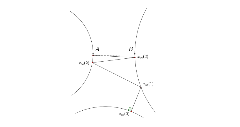
Figure 2. Period two orbit and an approximating homoclinic

For $j\in\{1,2\}$, we denote by $\mathrm{E}_{\mathcal{F}^{2}}^{s}(0_{j},0):=\{v\in T_{(0_{j},0)}\mathcal{M}:D_{(0_{j},0)}\mathcal{F}^{2}\cdot v=\lambda v\}$ the stable space of $\mathcal{F}^{2}$ at $(0_{j},0)$, associated to the smallest eigenvalue $\lambda<1$ of $(12)$. In the following, given two sequences $(u_{k})_{k\geq 0}$ and $(v_{k})_{k\geq 0}$ such that $v_{k}\neq 0$ for $k\geq k_{0}$, for some integer $k_{0}\geq 0$, we write $u_{k}\sim v_{k}$ if $\lim_{k\to+\infty}\frac{u_{k}}{v_{k}}=1$.

Lemma 3.5.

The orbit $h_{\infty}$ is homoclinic to the period two orbit $(12)$. More precisely, there exist two vectors $\bar{v}^{s}_{1}\in\mathrm{E}_{\mathcal{F}^{2}}^{s}(0_{1},0)$, $\bar{v}^{s}_{2}\in\mathrm{E}_{\mathcal{F}^{2}}^{s}(0_{2},0)$, with $\|\bar{v}_{1}^{s}\|=1$, and $\bar{v}_{2}^{s}=D_{(0_{1},0)}\mathcal{F}\cdot\bar{v}_{1}^{s}$, such that for $k\gg 1$, the following estimates hold:

$$x_{\infty}(2k)=(s_{\infty}(2k),\varphi_{\infty}(2k)) \sim\|x_{\infty}(2k)\|\bar{v}_{1}^{s},$$

$$x_{\infty}(2k+1)=(s_{\infty}(2k+1),\varphi_{\infty}(2k+1)) \sim\|x_{\infty}(2k)\|\bar{v}_{2}^{s},$$

with

$$\|x_{\infty}(2k)\|=O(\Lambda^{-2k}).$$

Proof.

As in Lemma 3.1, this is a consequences of the expansivity of the dynamics of $\mathcal{F}$ and of the fact that the forward orbits of $h_{\infty}$ and $(12)$ have the same symbolic coding. More precisely, for each integer $k\geq 1$, we let $[0,s_{\infty}(2k)]\ni s\mapsto\varphi^{(2k)}(s)$ be a continuous monotonic map such that $\varphi^{(2k)}(0)=0$ and $\varphi^{(2k)}(s_{\infty}(2k))=-\varphi_{\infty}(2k)$, and we set $\mathcal{W}^{(2k)}:=\{x^{(2k)}(s):=(s,\varphi^{(2k)}(s)):0\leq s\leq s_{\infty}(2k)\}$. By the strict convexity of the obstacles, $\mathcal{W}^{(2k)}$ is a dispersing wave front, and for each $0\leq j\leq k-1$, the projection of $\mathcal{F}^{2j}(\mathcal{W}^{(2k)})$ on the table is the arc of $\Gamma_{1}$ bounded by the points $A$ and $\gamma_{1}(s_{\infty}(k-j))$. Indeed, $\mathcal{F}^{2j}(s_{\infty}(2k),-\varphi_{\infty}(2k))=\mathcal{F}^{2j}\circ\mathcal{I}(x_{\infty}(2k))=\mathcal{I}\circ\mathcal{F}^{2(k-j)}(x_{\infty}(0))=(s_{\infty}(2(k-j)),-\varphi_{\infty}(2(k-j)))$. As before, we obtain

$$C \geq|\mathcal{F}^{2j}(\mathcal{W}^{(2k)})|=\left|\int_{0}^{s_{\infty}(2k)}\|D_{x^{(2k)}(s)}\mathcal{F}^{2j}\cdot(x^{(2k)})^{\prime}(s)\|_{p}\,ds\right|$$

$$\geq\Lambda^{2j}\left|\int_{0}^{s_{\infty}(2k)}\|(x^{(2k)})^{\prime}(s)\|_{p}\,ds\right|\geq\Lambda^{2j}c_{\text{min}}^{-1}\cdot\|x^{(2k)}(s_{\infty}(2k))-x^{(2k)}(0)\|,$$

and then,

(7) $$\|x_{\infty}(2k)\|\leq c_{\text{min}}C\Lambda^{-2k}.$$

In particular, $\lim_{k\to+\infty}\|x_{\infty}(2k)\|=0$, and then,

$$\lim_{k\to+\infty}\frac{x_{\infty}(2k)}{\|x_{\infty}(2k)\|}=:\bar{v}^{s}_{1},$$

for some unit vector $\bar{v}^{s}_{1}\in\mathrm{E}_{\mathcal{F}^{2}}^{s}(0_{1},0)$.

For any integer $k\geq 0$, we also have

$$x_{\infty}(2k+1) =\mathcal{F}(x_{\infty}(2k))-\mathcal{F}(0_{1},0)$$

$$\sim D_{(0_{1},0)}\mathcal{F}\cdot x_{\infty}(2k)$$

$$\sim D_{(0_{1},0)}\mathcal{F}\cdot\|x_{\infty}(2k)\|\bar{v}_{s}^{1}$$

$$=\|x_{\infty}(2k)\|\bar{v}_{2}^{s},$$

with $\bar{v}_{2}^{s}:=D_{(0_{1},0)}\mathcal{F}\cdot\bar{v}_{s}^{1}\in\mathrm{E}_{\mathcal{F}^{2}}^{s}(0_{2},0)$. ∎

4. Improved estimates on the parameters

In this part, we keep the same notations as previously, and we get improved estimates using a change of coordinates.

For $j\in\{1,2\}$, the point $(0_{j},0)$ is a saddle fixed point of $\mathcal{F}^{2}$, with eigenvalues $\lambda=\lambda(12)<1$ and $\mu=\mu(12):=\lambda^{-1}>1$. We denote by

$$\mathrm{E}_{\mathcal{F}^{2}}^{s}(0_{j},0) :=\{v\in T_{(0_{j},0)}\mathcal{M}:D_{(0_{j},0)}\mathcal{F}^{2}\cdot v=\lambda v\},$$

$$\mathrm{E}_{\mathcal{F}^{2}}^{u}(0_{j},0) :=\{v\in T_{(0_{j},0)}\mathcal{M}:D_{(0_{j},0)}\mathcal{F}^{2}\cdot v=\lambda^{-1}v\},$$

the stable, resp. unstable space of $\mathcal{F}^{2}$ at $(0_{j},0)$, associated to the smallest eigenvalue $\lambda<1$, resp. largest eigenvalue $\mu>1$ of $(12)$.

The rest of this section is dedicated to the proof of the following result.

Proposition 4.1.

There exist a real number $\xi_{\infty}\in{\mathbb{R}}$ and two vectors $v_{1}^{s}\in\mathrm{E}_{\mathcal{F}^{2}}^{s}(0_{1},0)$, $v_{2}^{s}\in\mathrm{E}_{\mathcal{F}^{2}}^{s}(0_{2},0)$, with $\|v_{1}^{s}\|=1$ and $v_{2}^{s}:=D_{(0_{1},0)}\mathcal{F}\cdot v_{1}^{s}$, such that for each integer $k\geq 0$, it holds

$$x_{\infty}(2k)=\lambda^{k}\xi_{\infty}\cdot v_{1}^{s}+O(\lambda^{\frac{3k}{2}}),$$

$$x_{\infty}(2k+1)=\lambda^{k}\xi_{\infty}\cdot v_{2}^{s}+O(\lambda^{\frac{3k}{2}}).$$

Furthermore, there exist an integer $n_{0}\geq 0$ and two vectors $v_{1}^{u}\in\mathrm{E}^{u}_{\mathcal{F}^{2}}(0_{1},0)$ and $v_{2}^{u}:=D_{(0_{1},0)}\mathcal{F}\cdot v_{1}^{u}\in\mathrm{E}^{u}_{\mathcal{F}^{2}}(0_{2},0)$ such that for each integer $n\geq n_{0}$, and for each integer $k\in\{0,\dots,\lceil\frac{n+1}{2}\rceil\}$, it holds

$$x_{n}(2k)-x_{\infty}(2k) =\lambda^{n+1-k}\xi_{\infty}\cdot v_{1}^{u}+O(\lambda^{n-\frac{k}{2}}),$$

$$x_{n}(2k+1)-x_{\infty}(2k+1) =\lambda^{n+1-k}\xi_{\infty}\cdot v_{2}^{u}+O(\lambda^{n-\frac{k}{2}}).$$

The proof of this proposition is given in Corollary 4.2 and Corollary 4.5 below.

4.1. The linearization near a saddle fixed point

The points $(0_{1},0)$ and $(0_{2},0)$ are saddle fixed points of the square $\mathcal{F}^{2}$ of the billiard map. For $n\geq 0$ large enough, and for each sufficiently large integer $k\in\{0,\dots,n+1\}$, the point $x_{n}(k)$ is in a neighborhood of one of those two points. To obtain the estimates of Proposition 4.1, we use a change of coordinates as follows to linearize the dynamics.

By Lemma 23 in [HKS], for any $\varepsilon>0$, there exist a neighborhood $\mathcal{U}$ of $(0_{1},0)$ in the $(s,\varphi)$-plane, a neighborhood $\mathcal{V}\subset{\mathbb{R}}^{2}$ of $(0,0)$, and a $C^{1,\frac{1}{2}}$-diffeomorphism

$$\Phi\colon\left\{\begin{array}[]{rcl}\mathcal{U}&\to&\mathcal{V},\\ (s,\varphi)&\mapsto&(\xi,\eta),\end{array}\right.$$

such that

$$\Phi\circ\mathcal{F}^{2}\circ\Phi^{-1}=D_{(0_{1},0)}\mathcal{F}^{2},\qquad\|\Phi-\mathrm{id}\|_{C^{1}}\leq\varepsilon,\qquad\|\Phi^{-1}-\mathrm{id}\|_{C^{1}}\leq\varepsilon,$$

and

$$\Phi(z)-\Phi(z^{\prime})=z-z^{\prime}+O(\max(|z|^{\frac{1}{2}},|z^{\prime}|^{\frac{1}{2}})|z-z^{\prime}|).$$

Let $L_{1}=L_{1}(\mathcal{F})\in\mathrm{SL}(2,{\mathbb{R}})$ be a linear isomorphism such that $v_{1}^{s}:=L_{1}^{-1}(1,0)\in\mathrm{E}_{\mathcal{F}^{2}}^{s}(0_{1},0)$, with $\|v_{1}^{s}\|=1$, and $L_{1}^{-1}(0,1)\in\mathrm{E}_{\mathcal{F}^{2}}^{u}(0_{1},0)$. By considering $\Psi:=L_{1}\circ\Phi$, with $\Phi$ as above, we deduce that for any $\varepsilon>0$, there exist a neighborhood $\mathcal{U}$ of $(0_{1},0)$, a neighborhood $\mathcal{V}$ of $(0,0)$, and a $C^{1,\frac{1}{2}}$-diffeomorphism $\Psi\colon\mathcal{U}\to\mathcal{V}$, such that

(8) $$\Psi\circ\mathcal{F}^{2}\circ\Psi^{-1}=D_{\lambda},\qquad\|\Psi-L_{1}\|_{C^{1}}\leq\varepsilon,\qquad\|\Psi^{-1}-L_{1}^{-1}\|_{C^{1}}\leq\varepsilon,$$

and

(9) $$\Psi(z)-\Psi(z^{\prime}) =L_{1}(z-z^{\prime})+O(\max(|z|^{\frac{1}{2}},|z^{\prime}|^{\frac{1}{2}})|z-z^{\prime}|),$$

$$\Psi^{-1}(z)-\Psi^{-1}(z^{\prime}) =L_{1}^{-1}(z-z^{\prime})+O(\max(|z|^{\frac{1}{2}},|z^{\prime}|^{\frac{1}{2}})|z-z^{\prime}|),$$

where $D_{\lambda}:=\mathrm{diag}(\lambda,\lambda^{-1})\colon(\xi,\eta)\mapsto(\lambda\xi,\lambda^{-1}\eta)$. Recall that $\mathcal{I}\colon(s,\varphi)\mapsto(s,-\varphi)$. Set $\mathcal{I}^{*}:=\Psi\circ\mathcal{I}\circ\Psi^{-1}$, and let $L_{2}=L_{2}(\mathcal{F})\in\mathrm{SL}(2,{\mathbb{R}})$ be the linear isomorphism (in fact, a reflection)

(10) $$L_{2}:=L_{1}\circ\mathcal{I}\circ L_{1}^{-1}.$$

Note that $\mathcal{I}^{*}(0,0)=(0,0)$. Then, we also have

(11) $$\mathcal{I}^{*}(z)-\mathcal{I}^{*}(z^{\prime})=L_{2}(z-z^{\prime})+O(\max(|z|^{\frac{1}{2}},|z^{\prime}|^{\frac{1}{2}})|z-z^{\prime}|).$$

In particular, $L_{2}$ is the linear part of $\mathcal{I}^{*}$ at the point $(0,0)$, i.e., $D_{(0,0)}\mathcal{I}^{*}=L_{2}$, and $\mathcal{I}^{*}(z)=L_{2}(z)+O(|z|^{\frac{3}{2}})$.

By Corollary 3.5 and Lemma 3.4, there exist $k_{0},n_{0}\geq 0$ such that for $n\geq n_{0}$, and for all $k\in\{k_{0},\dots,n+1-k_{0}\}$, the point $x_{n}(2k)$ is in the neighborhood $\mathcal{U}$ of $(0_{1},0)$. We denote by $(\xi_{n}(2k),\eta_{n}(2k))$ the coordinates of the point $\Psi(x_{n}(2k))$. It is possible to extend the system of coordinates given by $\Psi$ to a neighborhood of the separatrices as follows: for $k\in\{0,\dots,k_{0}-1\}$, we let

$$\Psi(x_{n}(2k))=(\xi_{n}(2k),\eta_{n}(2k)):=(\lambda^{k-k_{0}}\xi_{n}(2k_{0}),\lambda^{k_{0}-k}\eta_{n}(2k_{0})),$$

and analogously for $k\in\{n+1-k_{0}+1,\dots,n\}$. Let us abbreviate

$$(\xi_{n},\eta_{n}):=(\xi_{n}(0),\eta_{n}(0))=\Psi(x_{n}(0)),$$

so that

$$(\xi_{n}(2k),\eta_{n}(2k))=(\lambda^{k}\xi_{n},\lambda^{-k}\eta_{n}),\quad\forall\,k\in\{0,\dots,n\}.$$

By Lemma 3.5, the points $(x_{\infty}(k))_{k\geq 0}$ are on the stable manifold of $(0_{1},0)$. Therefore, their images by $\Psi$ are on the stable manifold of the origin, which is here the horizontal axis $\{\eta=0\}$. In our extended system of coordinates, we then have

$$\Psi(x_{\infty}(2k))=(\xi_{\infty}(2k),0)=(\lambda^{k}\xi_{\infty},0),\quad\forall\,k\geq 0,$$

for some $\xi_{\infty}\in{\mathbb{R}}$.

4.2. Proof of Proposition 4.1

In this part, we keep the same notations as before. Thanks to the above conjugacy, we can improve the estimates shown in Lemma 3.5.

Corollary 4.2.

Let $v_{1}^{s}=L_{1}^{-1}(1,0)\in\mathrm{E}_{\mathcal{F}^{2}}^{s}(0_{1},0)$ be as above, and set $v_{2}^{s}:=D_{(0_{1},0)}\mathcal{F}\cdot v_{1}^{s}\in\mathrm{E}_{\mathcal{F}^{2}}^{s}(0_{2},0)$. Then, we have the estimates

$$x_{\infty}(2k)=\lambda^{k}\xi_{\infty}\cdot v_{1}^{s}+O(\lambda^{\frac{3k}{2}}),$$

$$x_{\infty}(2k+1)=\lambda^{k}\xi_{\infty}\cdot v_{2}^{s}+O(\lambda^{\frac{3k}{2}}).$$

For $j=1,2$, we also have $v_{j}^{s}=\bar{v}_{j}^{s}$, with $\bar{v}_{j}^{s}$ as in Lemma 3.5.

Proof.

By (9), for each $k\geq 0$, we have

$$x_{\infty}(2k) =x_{\infty}(2k)-(0_{1},0)=\Psi^{-1}(\xi(2k),0)-\Psi^{-1}(0,0)$$

$$=\Psi^{-1}(\lambda^{k}\xi_{\infty},0)-\Psi^{-1}(0,0)$$

$$=\lambda^{k}\xi_{\infty}\cdot L_{1}^{-1}(1,0)+O(\lambda^{\frac{3k}{2}}).$$

By comparing with the estimates of Lemma 3.5, and since $v_{1}^{s}=L_{1}^{-1}(1,0)$ is taken to be of norm one, we see that $v_{1}^{s}=\bar{v}_{1}^{s}$.

Then, for odd integers, in the same way as before, we obtain

$$x_{\infty}(2k+1) =\mathcal{F}(x_{\infty}(2k))-\mathcal{F}(0_{1},0)=D_{(0_{1},0)}\mathcal{F}\cdot x_{\infty}(2k)+O(\lambda^{2k})$$

$$=\lambda^{k}\xi_{\infty}\,D_{(0_{1},0)}\mathcal{F}\cdot v_{1}^{s}+O(\lambda^{\frac{3k}{2}}),$$

which concludes. ∎

Recall that $\mathcal{I}\colon(s,\varphi)\mapsto(s,-\varphi)$, and that $\mathcal{I}\circ\mathcal{F}\circ\mathcal{I}=\mathcal{F}^{-1}$. Besides, we let $\mathcal{I}^{*}:=\Psi\circ\mathcal{I}\circ\Psi^{-1}$, and we let $L_{2}=L_{2}(\mathcal{F}):=L_{1}\circ\mathcal{I}\circ L_{1}^{-1}\in\mathrm{SL}(2,{\mathbb{R}})$ be as in (10).

Lemma 4.3.

For some $\alpha\in{\mathbb{R}}^{*}$, we have

$$L_{2}(\xi,\eta)=(\alpha^{-1}\eta,\alpha\xi),\qquad\forall\,(\xi,\eta)\in{\mathbb{R}}^{2}.$$

Proof.

We have $\mathcal{I}\circ\mathcal{F}^{2}\circ\mathcal{I}=\mathcal{F}^{-2}$. By (8) and the definition of $\mathcal{I}^{*}$, we thus obtain $\mathcal{I}^{*}\circ D_{\lambda}\circ\mathcal{I}^{*}=D_{\lambda}^{-1}$. Then, by (11), and since $\mathcal{I}^{*}(0,0)=(0,0)$, we deduce that $L_{2}\circ D_{\lambda}\circ L_{2}(z)=D_{\lambda}^{-1}(z)+O(|z|^{\frac{3}{2}})$, for all $z\in{\mathbb{R}}^{2}$. But the maps $L_{2}=L_{1}\circ\mathcal{I}\circ L_{1}^{-1}\in\mathrm{SL}(2,{\mathbb{R}})$ and $D_{\lambda}$ are linear. Therefore, by identifying the linear parts, we get $L_{2}\circ D_{\lambda}\circ L_{2}=D_{\lambda}^{-1}$. Now, we also have $\mathcal{I}_{0}\circ D_{\lambda}\circ\mathcal{I}_{0}=D_{\lambda}^{-1}$, with $\mathcal{I}_{0}\colon(\xi,\eta)\mapsto(\eta,\xi)$, hence $\mathcal{I}_{0}\circ L_{2}\in\mathrm{SL}(2,{\mathbb{R}})$ commutes with the diagonal matrix $D_{\lambda}$. Since the $\mathrm{SL}(2,{\mathbb{R}})$-centralizer of $D_{\lambda}$ is reduced to the subset of diagonal matrices in $\mathrm{SL}(2,{\mathbb{R}})$, we conclude that $L_{2}=\mathcal{I}_{0}\circ D_{\alpha}\colon(\xi,\eta)\mapsto(\alpha^{-1}\eta,\alpha\xi)$, for some $\alpha\in{\mathbb{R}}^{*}$. ∎

Lemma 4.4.

Let $n\geq n_{0}$. It holds

(12) $$\eta_{n}=\alpha\lambda^{n+1}\xi_{n}+O(\lambda^{\frac{5n}{4}}),\qquad\xi_{n}=\xi_{\infty}(1+\lambda^{n+1})+O(\lambda^{\frac{5n}{4}}).$$

Then, for any $k\in\{0,\dots,n+1\}$, we have

(13) $$\Psi(x_{n}(2k))=(\lambda^{k}\xi_{n},\lambda^{-k}\eta_{n})=\xi_{\infty}(\lambda^{k}+\lambda^{n+1+k},\alpha\lambda^{n+1-k})+O(\lambda^{\frac{5n}{4}-k}).$$

Proof.

Let $n\geq n_{0}$, and let $k\in\{0,\dots,n+1\}$. We obtain successively

$$(\lambda^{n+1-k}\xi_{n},\lambda^{k-n-1}\eta_{n}) =(\xi_{n}(2n+2-2k),\eta_{n}(2n+2-2k))$$

$$=\Psi\circ\mathcal{F}^{2n+2-2k}(x_{n}(0))$$

$$=\Psi\circ\mathcal{F}^{2n+2-2k}\circ\mathcal{I}(x_{n}(0))$$

$$=\Psi\circ\mathcal{I}\circ\mathcal{F}^{2k-2n-2}(x_{n}(0))$$

$$=(\Psi\circ\mathcal{I}\circ\Psi^{-1})\circ\Psi(\mathcal{F}^{2k}(x_{n}(0)))$$

$$=\mathcal{I}^{*}(\xi_{n}(2k),\eta_{n}(2k))-\mathcal{I}^{*}(0,0)$$

$$=L_{2}(\lambda^{k}\xi_{n},\lambda^{-k}\eta_{n})+O(\|(\lambda^{k}\xi_{n},\lambda^{-k}\eta_{n})\|^{\frac{3}{2}})$$

$$=(\alpha^{-1}\lambda^{-k}\eta_{n},\alpha\lambda^{k}\xi_{n})+\lambda^{\frac{3k}{2}}\cdot O(\|(\xi_{n},\lambda^{-2k}\eta_{n})\|^{\frac{3}{2}}).$$

Indeed, we have $\mathcal{I}(x_{n}(0))=\mathcal{I}(s_{n}(0),0)=(s_{n}(0),0)=x_{n}(0)$, and $\mathcal{F}^{2k-2n-2}(x_{n}(0))=\mathcal{F}^{2k}(x_{n}(0))$, by the $(2n+2)$-periodicity of $h_{n}$. Here, we have also used that $\mathcal{I}^{*}(0,0)=(0,0)$. Then, the last two lines above follow from (11) and Lemma 4.3.

Multiplying by $\alpha\lambda^{k}$, and projecting on the first component, we deduce that $\eta_{n}=\alpha\lambda^{n+1}\xi_{n}+\lambda^{\frac{5k}{2}}\cdot O(\|(\xi_{n},\lambda^{-2k}\eta_{n})\|^{\frac{3}{2}})$. Letting $k:=\lceil\frac{n}{2}\rceil$, we thus obtain $\eta_{n}=\alpha\lambda^{n+1}\xi_{n}+\lambda^{\frac{5n}{4}}\cdot O(\|(\xi_{n},\lambda^{-n}\eta_{n})\|^{\frac{3}{2}})=\alpha\lambda^{n+1}\xi_{n}+\lambda^{\frac{5n}{4}}\cdot O(|\xi_{n}|^{\frac{3}{2}})$, i.e.,

$$\eta_{n}=\alpha\lambda^{n+1}\xi_{n}+O(\lambda^{\frac{5n}{4}}),$$

which concludes the proof of the first estimate in (12).

For any $k\in\{0,\dots,n+1\}$, we thus have

(14) $$(\lambda^{k}\xi_{n},\lambda^{-k}\eta_{n})=\xi_{n}(\lambda^{k},\alpha\lambda^{n+1-k})+O(\lambda^{\frac{5n}{4}-k}).$$

Then, by linearity of $L_{2}$, and by (11), we obtain

$$(\alpha^{-1}\eta_{n},\alpha(\xi_{n}-\xi_{\infty})) =L_{2}(\xi_{n}-\xi_{\infty},\eta_{n})$$

$$=L_{2}(\xi_{n},\eta_{n})-L_{2}(\xi_{\infty},0)$$

$$=\mathcal{I}^{*}(\xi_{n},\eta_{n})-\mathcal{I}^{*}(\xi_{\infty},0)+O(\|(\xi_{n}-\xi_{\infty},\eta_{n})\|^{\frac{3}{2}})$$

$$=\Psi\circ\mathcal{I}(s_{n}(0),0)-\Psi\circ\mathcal{I}(s_{\infty}(0),0)+O(\|(\xi_{n}-\xi_{\infty},\eta_{n})\|^{\frac{3}{2}})$$

$$=\Psi(s_{n}(0),0)-\Psi(s_{\infty}(0),0)+O(\|(\xi_{n}-\xi_{\infty},\eta_{n})\|^{\frac{3}{2}})$$

$$=(\xi_{n},\eta_{n})-(\xi_{\infty},0)+O(\|(\xi_{n}-\xi_{\infty},\eta_{n})\|^{\frac{3}{2}})$$

$$=(\xi_{n}-\xi_{\infty},\eta_{n})+O(\|(\xi_{n}-\xi_{\infty},\eta_{n})\|^{\frac{3}{2}}).$$

The estimate of the error term above follows from the fact that $\mathcal{I}^{*}(z)=L_{2}(z)+O(|z|^{\frac{3}{2}})$, and from the definition of the extension of our system of coordinates to a neighborhood of the separatrix (the differential of $\mathcal{I}^{*}$ at points which are on the separatrix is equal to $L_{2}$). Projecting on the first component, we thus obtain $\lambda^{n+1}\xi_{n}=\alpha^{-1}\eta_{n}+O(\lambda^{\frac{5n}{4}})=\xi_{n}-\xi_{\infty}+O(\lambda^{\frac{5n}{4}})$, hence

$$\xi_{n}=\frac{\xi_{\infty}}{1-\lambda^{n+1}}+O(\lambda^{\frac{5n}{4}})=\xi_{\infty}(1+\lambda^{n+1})+O(\lambda^{\frac{5n}{4}}),$$

which gives the second estimate in (12). Combining this with (14), this concludes the proof of (13). ∎

Corollary 4.5.

Let $v_{1}^{u}:=\alpha L_{1}^{-1}(0,1)\in\mathrm{E}^{u}_{\mathcal{F}^{2}}(0_{1},0)$, and set $v_{2}^{u}:=D_{(0_{1},0)}\mathcal{F}\cdot v_{1}^{u}\in\mathrm{E}^{u}_{\mathcal{F}^{2}}(0_{2},0)$. Then, for each $n\geq n_{0}$, and for each $k\in\{0,\dots,\lceil\frac{n+1}{2}\rceil\}$, we have

$$x_{n}(2k)-x_{\infty}(2k) =\lambda^{n+1-k}\xi_{\infty}\cdot v_{1}^{u}+O(\lambda^{n-\frac{k}{2}}),$$

$$x_{n}(2k+1)-x_{\infty}(2k+1) =\lambda^{n+1-k}\xi_{\infty}\cdot v_{2}^{u}+O(\lambda^{n-\frac{k}{2}}).$$

Proof.

Let $k\in\{0,\dots,\lceil\frac{n+1}{2}\rceil\}$. Recall that $\Psi(x_{\infty}(2k))=(\lambda^{k}\xi_{\infty},0)$. Therefore, we deduce from (13) that

$$\Psi(x_{n}(2k))-\Psi(x_{\infty}(2k)) =\xi_{\infty}(\lambda^{n+1+k},\alpha\lambda^{n+1-k})+O(\lambda^{\frac{5n}{4}-k})$$

$$=\alpha\lambda^{n+1-k}\xi_{\infty}(\alpha^{-1}\lambda^{2k},1)+O(\lambda^{\frac{5n}{4}-k}).$$

By (9), and since $0\leq k\leq\lceil\frac{n+1}{2}\rceil$, we conclude that

$$x_{n}(2k)-x_{\infty}(2k)=\lambda^{n+1-k}\xi_{\infty}\cdot\alpha L_{1}^{-1}(0,1)+O(\lambda^{n-\frac{k}{2}}).$$

We have $(0,1)\in\mathrm{E}_{D_{\lambda}}^{u}(0,0)$, and $L_{1}^{-1}(0,1)\in\mathrm{E}_{\mathcal{F}^{2}}^{u}(0_{1},0)$. Set $v_{1}^{u}:=\alpha L_{1}^{-1}(0,1)$. We have $v_{1}^{u}\in\mathrm{E}_{\mathcal{F}^{2}}^{u}(0_{1},0)$, and for each $k\in\{0,\dots,\lceil\frac{n+1}{2}\rceil\}$, it holds

$$x_{n}(2k)-x_{\infty}(2k)=\lambda^{n+1-k}\xi_{\infty}\cdot v_{1}^{u}+O(\lambda^{n-\frac{k}{2}}).$$

Applying $\mathcal{F}$, we get

$$x_{n}(2k+1)-x_{\infty}(2k+1) =\mathcal{F}(x_{n}(2k))-\mathcal{F}(x_{\infty}(2k))$$

$$=D_{(0_{1},0)}\mathcal{F}\cdot(x_{n}(2k)-x_{\infty}(2k))+O(\lambda^{2(n+1-k)})$$

$$=\lambda^{n+1-k}\xi_{\infty}\,D_{(0_{1},0)}\mathcal{F}\cdot v_{1}^{u}+O(\lambda^{n-\frac{k}{2}}),$$

with $D_{(0_{1},0)}\mathcal{F}\cdot v_{1}^{u}=:v_{2}^{u}$, and $v_{2}^{u}\in D_{(0_{1},0)}\mathcal{F}\cdot\mathrm{E}_{\mathcal{F}^{2}}^{u}(0_{1},0)=\mathrm{E}_{\mathcal{F}^{2}}^{u}(0_{2},0)$. ∎

Remark 4.6.

It is also possible to derive the previous result (Lemma 4.4) by more geometric arguments. In the rest of this section, we explain how similar estimates can be obtained by considering the growth of certain dispersing waves fronts.

Given $n\geq 0$, we consider the dispersing wave front $\mathcal{W}_{n,\infty}(0):=\{x(s):=(s,0):s_{n}\leq s\leq S_{n}\}$, where $s_{n}:=\min(s_{n}(0),s_{\infty}(0))$, and $S_{n}:=\max(s_{n}(0),s_{\infty}(0))$. In other terms, $\mathcal{W}_{n,\infty}(0)$ is the arc of $\Gamma_{3}$ connecting the points with respective parameters $s_{n}(0)$ and $s_{\infty}(0)$, each point being endowed with $0$ angle. Given any $x=(s,0)\in\mathcal{W}_{n,\infty}(0)$, we denote by $x(s,k)$, $0\leq k\leq 2n+1$, its forward iterates.

Figure 3. Approximating periodic and homoclinic orbits

The respective symbolic codings of the forward orbits of $x_{n}(0)$ and $x_{\infty}(0)$ are

$$3\underbrace{21212\dots 21212}_{2n+1}321\dots,\qquad 3\underbrace{21212\dots 21212}_{2n+1}121\dots,$$

By strict convexity, it follows that for any $1\leq k\leq n$, $\mathcal{W}_{n,\infty}(2k):=\mathcal{F}^{2k}(\mathcal{W}_{n,\infty})$ is a dispersing wave front whose projection on the configuration space is the arc of $\Gamma_{1}$ between the points with respective parameters $s_{n}(2k)$ and $s_{\infty}(2k)$. In particular, we have $|\mathcal{W}_{n,\infty}(2k)|\leq C_{0}$, for some uniform constant $C_{0}>0$. Besides, by Lemma 3.5, we know that $\lim_{n\to+\infty}x_{\infty}(2n)=(0_{1},0)$, and by Corollary 3.4, we also have $\lim_{n\to+\infty}x_{n}(2n)=\mathcal{I}(x_{\infty}(2))=(s_{\infty}(2),-\varphi_{\infty}(2))$. Therefore, the sequence of wave fronts $(\mathcal{W}_{n,\infty}(2n))_{n\geq 0}$ converges pointwise, and there exists $W>0$ such that $\lim_{n\to+\infty}|\mathcal{W}_{n,\infty}(2n)|=W$.

Besides, for any $1\leq k\leq n$, it holds

$$|\mathcal{W}_{n,\infty}(2k)| =\int_{\mathcal{W}_{n,\infty}(0)}\|D_{x}\mathcal{F}^{2k}\cdot dx\|_{p}=\left|\int_{s_{n}(0)}^{s_{\infty}(0)}\|D_{(s,0)}\mathcal{F}^{2k}\cdot(1,0)\|_{p}\,ds\right|$$

$$=\int_{s_{n}}^{S_{n}}\left\|\prod_{j=0}^{k-1}D_{x(s,2j)}\mathcal{F}^{2}\cdot(1,0)\right\|_{p}\,ds.$$

On the one hand, the orbit $h_{\infty}=(x_{\infty}(k))_{k\geq 0}$ is homoclinic to the period two orbit $(12)$ whose Lyapunov exponent is equal to $\frac{1}{2}\log\mu$, where $\mu=\lambda^{-1}>1$. Since the $s$-coordinate corresponds to the position on the obstacles, whose curvature is nonzero, the vector $(1,0)$ has some non-vanishing component along the unstable direction. Thus, for $k=n$, we obtain

$$\left\|\prod_{j=0}^{n-1}D_{x(s_{\infty}(0),2j)}\mathcal{F}^{2}\cdot(1,0)\right\|_{p}=\left\|\prod_{j=0}^{n-1}D_{x_{\infty}(0)}\mathcal{F}^{2}\cdot(1,0)\right\|_{p}\sim K(s_{\infty}(0))\cdot\mu^{n},$$

for some constant $K(s_{\infty}(0))>0$.

On the other hand, by Corollary 3.4, we get

$$\left\|\prod_{j=0}^{n-1}D_{x_{n}(2j)}\mathcal{F}^{2}\cdot(1,0)\right\|_{p} \sim\left\|\prod_{j=\lceil\frac{n}{2}\rceil}^{2}D_{\mathcal{I}(x_{\infty}(2j))}\mathcal{F}^{2}\circ\prod_{j=0}^{\lceil\frac{n}{2}\rceil-1}D_{x_{\infty}(2j)}\mathcal{F}^{2}\cdot(1,0)\right\|_{p}$$

$$\sim K(s_{n}(0))\cdot\mu^{n},$$

for some constant $K(s_{n}(0))>0$.

Then, by strict convexity of the table, there exists a monotonic map $K_{n}\colon[s_{n},S_{n}]\to{\mathbb{R}}_{+}^{*}$, $t\mapsto K_{n}(t)$, such that $K_{n}(s_{n})=K(s_{n})$, $K_{n}(S_{n})=K(S_{n})$, and

$$\left\|\prod_{j=0}^{n-1}D_{x(s,2j)}\mathcal{F}^{2}\cdot(1,0)\right\|_{p}\sim K_{n}(s)\cdot\mu^{n}.$$

By Corollary 3.4, we have $\lim_{n\to+\infty}|\mathcal{W}_{n,\infty}(0)|=\lim_{n\to+\infty}(S_{n}-s_{n})=0$, and then,

$$W\sim|\mathcal{W}_{n,\infty}(2n)|\sim\left(\int_{s_{n}}^{S_{n}}K_{n}(s)\,ds\right)\cdot\mu^{n}\sim\left|s_{n}(0)-s_{\infty}(0)\right|\cdot K(s_{\infty}(0))\mu^{n}.$$

By the fact that $x_{n}(0)=(s_{n}(0),0)$ and $x_{\infty}(0)=(s_{\infty}(0),0)$, we deduce that

$$x_{n}(0)-x_{\infty}(0)\sim\lambda^{n}\cdot v,$$

for some vector $v\in{\mathbb{R}}^{2}$ with $\|v\|=K(s_{\infty}(0))^{-1}W>0$. In particular, we see that we recover the same kind of estimate as in Corollary 4.5, for $k=0$. To obtain estimates on the forward iterates $x_{\infty}(2k)$ and $x_{n}(2k)$, with $0\leq k\leq n$, we just have to apply the dynamics. For instance, we have

$$x_{n}(1)-x_{\infty}(1)=\mathcal{F}(x_{n}(0))-\mathcal{F}(x_{\infty}(0))\sim D_{x_{\infty}(0)}\mathcal{F}\cdot(x_{n}(0)-x_{\infty}(0)).$$

In the same way, by Corollary 3.4, for any $k\in\{0,\dots,n+1\}$, we get

$$x_{n}(k)-x_{\infty}(k)=\mathcal{F}^{k}(x_{n}(0))-\mathcal{F}^{k}(x_{\infty}(0))$$

$$\sim\prod_{j=0}^{k-1}D_{x_{\infty}(j)}\mathcal{F}\cdot(x_{n}(0)-x_{\infty}(0))=(s_{n}(0)-s_{\infty}(0))\cdot\prod_{j=0}^{k-1}D_{x_{\infty}(j)}\mathcal{F}\cdot(1,0).$$

With the notations introduced above, we get $\left\|\prod_{j=0}^{k-1}D_{x_{\infty}(2j)}\mathcal{F}^{2}\cdot(1,0)\right\|\sim K(s_{\infty}(0))\cdot\mu^{k}$. In analogy with Corollary 4.5, for $k\in\{0,\dots,n+1\}$, we thus have

$$\|x_{n}(2k)-x_{\infty}(2k)\|\sim W\cdot\lambda^{n-k}.$$

5. Consequences on the Marked Length Spectrum

5.1. Further remarks on the asymptotic constants

In this part, we want to relate the asymptotic constants associated to the vectors $v_{1}^{s},v_{2}^{s},v_{1}^{u},v_{2}^{u}$ defined above. Here, we let $v_{1}^{s}=L_{1}^{-1}(1,0)\in\mathrm{E}_{\mathcal{F}^{2}}^{s}(0_{1},0)$, $v_{2}^{s}=D_{(0_{1},0)}\mathcal{F}\cdot v_{1}^{s}\in\mathrm{E}_{\mathcal{F}^{2}}^{s}(0_{2},0)$ be as in Corollary 4.2, and we let $v_{1}^{u}:=\alpha L_{1}^{-1}(0,1)\in\mathrm{E}^{u}_{\mathcal{F}^{2}}(0_{1},0)$, $v_{2}^{u}=D_{(0_{1},0)}\mathcal{F}\cdot v_{1}^{u}\in\mathrm{E}^{u}_{\mathcal{F}^{2}}(0_{2},0)$ be as in Corollary 4.5.

Let us denote

$$v_{1}^{s}=(C_{1,s}^{s},C_{1,\varphi}^{s}), \qquad v_{2}^{s}=(C_{2,s}^{s},C_{2,\varphi}^{s}),$$

$$v_{1}^{u}=(C_{1,s}^{u},C_{1,\varphi}^{u}), \qquad v_{2}^{u}=(C_{2,s}^{u},C_{2,\varphi}^{u}),$$

and recall that for $\{i,j\}=\{1,2\}$, we have

(15) $$D_{(0_{i},0)}\mathcal{F}=-\begin{pmatrix}\frac{\ell}{R_{i}}+1&\ell\\ \frac{\ell}{R_{i}R_{j}}+\frac{1}{R_{i}}+\frac{1}{R_{j}}&\frac{\ell}{R_{j}}+1\end{pmatrix}=-\begin{pmatrix}\alpha_{i}&\ell\\ \gamma&\alpha_{j}\end{pmatrix},$$

with $\ell:=\frac{\mathcal{L}(12)}{2}=h(0_{1},0_{2})$, $\alpha_{1}:=\frac{\ell}{R_{1}}+1$, $\alpha_{2}:=\frac{\ell}{R_{2}}+1$, and $\gamma:=\ell^{-1}(\alpha_{1}\alpha_{2}-1)$.

In particular, we get

(16) $$D_{(0_{i},0)}\mathcal{F}^{2}=\begin{pmatrix}2\alpha_{1}\alpha_{2}-1&2\alpha_{j}\ell\\ 2\alpha_{i}\gamma&2\alpha_{1}\alpha_{2}-1\end{pmatrix}=\frac{1}{2}\begin{pmatrix}\lambda+\lambda^{-1}&4\alpha_{j}\ell\\ 4\alpha_{i}\gamma&\lambda+\lambda^{-1}\end{pmatrix}.$$

Indeed, we know that $\mathrm{tr}(D_{(0_{1},0)}\mathcal{F}^{2})=\mathrm{tr}(D_{(0_{2},0)}\mathcal{F}^{2})=\lambda+\lambda^{-1}$, since $\lambda,\lambda^{-1}$ are the common eigenvalues of $D_{(0_{1},0)}\mathcal{F}^{2}$ and $D_{(0_{2},0)}\mathcal{F}^{2}$.

Corollary 5.1.

We have

(17) $$\frac{C_{1,s}^{s}}{C_{1,\varphi}^{s}}=-\frac{4\alpha_{2}\lambda}{1-\lambda^{2}}\ell<0,\qquad\frac{C_{1,s}^{u}}{C_{1,\varphi}^{u}}=\frac{4\alpha_{2}\lambda}{1-\lambda^{2}}\ell>0,$$

and

(18) $$\frac{C_{2,s}^{s}}{C_{2,\varphi}^{s}}=-\frac{4\alpha_{1}\lambda}{1-\lambda^{2}}\ell<0,\qquad\frac{C_{2,s}^{u}}{C_{2,\varphi}^{u}}=\frac{4\alpha_{1}\lambda}{1-\lambda^{2}}\ell>0.$$

Moreover, we have

(19) $$\frac{C_{2,s}^{s}}{C_{1,\varphi}^{s}}=\frac{2\lambda}{1-\lambda}\ell>0,\qquad\frac{C_{2,s}^{u}}{C_{1,\varphi}^{u}}=-\frac{2}{1-\lambda}\ell<0.$$

Proof.

Since $v_{1}^{s}=(C_{1,s}^{s},C_{1,\varphi}^{s})\in\mathrm{E}_{\mathcal{F}^{2}}^{s}(0_{1},0)$, then by definition, and by (16), we have

$$\frac{\lambda+\lambda^{-1}}{2}C_{1,s}^{s}+2\alpha_{2}\ell C_{1,\varphi}^{s}=\lambda C_{1,s}^{s},$$

and the first equality of (17) follows. The second one is proved analogously, since $v_{1}^{u}=(C_{1,s}^{u},C_{1,\varphi}^{u})\in\mathrm{E}_{\mathcal{F}^{2}}^{u}(0_{1},0)$. We argue similarly for (18), since $v_{2}^{s}\in\mathrm{E}_{\mathcal{F}^{2}}^{s}(0_{2},0)$, and $v_{2}^{u}\in\mathrm{E}_{\mathcal{F}^{2}}^{u}(0_{2},0)$.

Now, by definition, we have $v_{2}^{s}=D_{(0_{1},0)}\mathcal{F}\cdot v_{1}^{s}$, and then, (15) and (17) yield

$$C_{2,s}^{s}=-\alpha_{1}C_{1,s}^{s}-\ell C_{1,\varphi}^{s}=\left(\frac{4\alpha_{1}\alpha_{2}}{\lambda^{-1}-\lambda}-1\right)\ell C_{1,\varphi}^{s}.$$

Moreover, by the definition of $D_{(0_{1},0)}\mathcal{F}^{2}$, we see that

(20) $$\mathrm{tr}(D_{(0_{1},0)}\mathcal{F}^{2})=4\alpha_{1}\alpha_{2}-2=\lambda+\lambda^{-1},$$

hence

$$\frac{C_{2,s}^{s}}{C_{1,\varphi}^{s}}=\frac{2(1+\lambda)}{\lambda^{-1}-\lambda}\ell=\frac{2(1+\lambda)}{\lambda^{-1}(1-\lambda^{2})}\ell=\frac{2\lambda}{1-\lambda}\ell.$$

Similarly, we have $v_{2}^{u}=D_{(0_{1},0)}\mathcal{F}\cdot v_{1}^{u}$, and

$$C_{2,s}^{u}=-\alpha_{1}C_{1,s}^{u}-\ell C_{1,\varphi}^{u}=-\left(\frac{4\alpha_{1}\alpha_{2}}{\lambda^{-1}-\lambda}+1\right)\ell C_{1,\varphi}^{u}=-\frac{2}{1-\lambda}\ell C_{1,\varphi}^{u},$$

which gives (19). ∎

Corollary 5.2.

The following relations hold between the asymptotic constants $C_{1,\varphi}^{s},C_{2,\varphi}^{s},C_{1,\varphi}^{u}$ and $C_{2,\varphi}^{u}$:

(21) $$\frac{C_{2,\varphi}^{s}}{C_{1,\varphi}^{s}}=-\frac{1+\lambda}{2\alpha_{1}},\qquad\quad\frac{C_{1,\varphi}^{u}}{C_{1,\varphi}^{s}}=-1,\qquad\quad\frac{C_{2,\varphi}^{u}}{C_{1,\varphi}^{s}}=\frac{1+\lambda^{-1}}{2\alpha_{1}}.$$

Since we will need it in the following, we also compute:

(22) $$\left(\frac{C_{2,\varphi}^{s}}{C_{1,\varphi}^{s}}\right)^{2}=\frac{\lambda\alpha_{2}}{\alpha_{1}},\qquad\quad\left(\frac{C_{2,\varphi}^{u}}{C_{1,\varphi}^{s}}\right)^{2}=\frac{\alpha_{2}}{\lambda\alpha_{1}}.$$

Proof.

The first equality follows immediately from (18) and (19), by writing

$$\frac{C_{2,\varphi}^{s}}{C_{1,\varphi}^{s}}=\frac{C_{2,\varphi}^{s}}{C_{2,s}^{s}}\cdot\frac{C_{2,s}^{s}}{C_{1,\varphi}^{s}}=-\frac{1-\lambda^{2}}{4\alpha_{1}\lambda}\cdot\frac{2\lambda}{1-\lambda}=-\frac{1+\lambda}{2\alpha_{1}}.$$

To prove the other identities, we argue as follows. Let us assume that $n=2m-1$, for some integer $m\geq 1$. By the estimates of Corollary 4.5, for $k=m$, we get

$$x_{n}(2m)-x_{\infty}(2m)\sim\lambda^{n+1-m}\xi_{\infty}\cdot v_{1}^{u}=\lambda^{m}\xi_{\infty}\cdot v_{1}^{u}.$$

By Lemma 3.2, we also have $x_{n}(n+1)=x_{n}(2m)=(s_{n}(2m),0)$, i.e., $\varphi_{n}(2m)=0$. Thus, by projecting the previous relation on the second coordinate, we get

(23) $$\varphi_{\infty}(2m)\sim-C_{1,\varphi}^{u}\cdot\lambda^{m}\xi_{\infty}.$$

On the other hand, by Corollary 4.2, we also have

$$x_{\infty}(2m)=(s_{\infty}(2m),\varphi_{\infty}(2m))\sim\lambda^{m}\xi_{\infty}\cdot v_{1}^{s},$$

and then, the projection of this relation on the second coordinate yields

$$\varphi_{\infty}(2m)\sim C_{1,\varphi}^{s}\cdot\lambda^{m}\xi_{\infty}.$$

Combining this with (23), we obtain

(24) $$\frac{C_{1,\varphi}^{u}}{C_{1,\varphi}^{s}}=-1,$$

which gives the second equality in (21).

Let us show the last one. By (18), (19) and (24), we get

$$\frac{C_{2,\varphi}^{u}}{C_{1,\varphi}^{s}}=\frac{C_{2,\varphi}^{u}}{C_{2,s}^{u}}\cdot\frac{C_{2,s}^{u}}{C_{1,\varphi}^{u}}\cdot\frac{C_{1,\varphi}^{u}}{C_{1,\varphi}^{s}}=\frac{1-\lambda^{2}}{4\alpha_{1}\lambda}\cdot\left(-\frac{2}{1-\lambda}\right)\cdot(-1)=\frac{1+\lambda}{2\alpha_{1}\lambda},$$

which concludes the proof of (21).

To show (22), we use the fact that $\lambda+\lambda^{-1}+2=4\alpha_{1}\alpha_{2}$. Also, by (21), we have $\frac{C_{2,\varphi}^{s}}{C_{2,\varphi}^{u}}=-\lambda$. We get

$$\left(\frac{C_{2,\varphi}^{s}}{C_{1,\varphi}^{s}}\right)^{2}=\lambda^{2}\left(\frac{C_{2,\varphi}^{u}}{C_{1,\varphi}^{s}}\right)^{2}=\frac{1+2\lambda+\lambda^{2}}{4\alpha_{1}^{2}}=\lambda\cdot\frac{\lambda+2+\lambda^{-1}}{4\alpha_{1}^{2}}=\lambda\cdot\frac{4\alpha_{1}\alpha_{2}}{4\alpha_{1}^{2}}=\frac{\lambda\alpha_{2}}{\alpha_{1}}.$$

∎

5.2. Computing the $2$-jet of the generating function

Recall that the function $h\colon(s,s^{\prime})\mapsto\|\gamma(s)-\gamma(s^{\prime})\|$ is generating for the billiard map $\mathcal{F}\colon(s,\varphi)\mapsto(s^{\prime},\varphi^{\prime})$. In other terms, for the $1$-form $\omega:=-\sin(\varphi)ds$, we have

$$\mathcal{F}^{*}\omega-\omega=dh(s,s^{\prime}).$$

In the following, given a point $\gamma(s)\in\partial\mathcal{D}$ in the boundary of the table, we denote by $R(s)>0$ the radius of curvature at $\gamma(s)$, defined as the radius of the osculating circle at this point. We also have $R(s)=\mathcal{K}(s)^{-1}$, where $\mathcal{K}(s)$ is the curvature. In the following lemma, we compute the second order Taylor expansion of the function $h$. Given $x=(s,\varphi)\in\mathcal{M}$ with $\mathcal{F}(s,\varphi)=(s^{\prime},\varphi^{\prime})$, we set

(25) $$\zeta^{-}(x):=\frac{R(s)\cos(\varphi)}{h(s,s^{\prime})},\qquad\zeta^{+}(x):=\frac{R(s^{\prime})\cos(\varphi^{\prime})}{h(s,s^{\prime})}.$$

Lemma 5.3.

Let $x=(s,\varphi)$, $\bar{x}=(\bar{s},\bar{\varphi})\in\mathcal{M}$ be close to each other. We set $x^{\prime}=(s^{\prime},\varphi^{\prime}):=\mathcal{F}(s,\varphi)$, and $\bar{x}^{\prime}=(\bar{s}^{\prime},\bar{\varphi}^{\prime}):=\mathcal{F}(\bar{s},\bar{\varphi})$. Then, we get

$$\quad h(\bar{s},\bar{s}^{\prime})-h(s,s^{\prime})=R(s)\sin(\varphi)(\varphi-\bar{\varphi})+R(s^{\prime})\sin(\varphi^{\prime})(\varphi^{\prime}-\bar{\varphi}^{\prime})$$

$$\quad+\frac{h(s,s^{\prime})}{2}\left(\zeta^{-}(x)\left(1+\zeta^{-}(x)\right)\cdot(\varphi-\bar{\varphi})^{2}+\zeta^{+}(x)\left(1+\zeta^{+}(x)\right)\cdot(\varphi^{\prime}-\bar{\varphi}^{\prime})^{2}\right.$$

$$\quad\left.+2\zeta^{-}(x)\zeta^{+}(x)\cdot(\varphi-\bar{\varphi})(\varphi^{\prime}-\bar{\varphi}^{\prime})+O(\|\bar{x}-x\|^{3})\right).$$

Proof.

Assume that $x=(s,\varphi)\in\mathcal{M}$ and $\bar{x}=(\bar{s},\bar{\varphi})\in\mathcal{M}$ are close to each other, and let $(s^{\prime},\varphi^{\prime}):=\mathcal{F}(s,\varphi)$, and $(\bar{s}^{\prime},\bar{\varphi}^{\prime}):=\mathcal{F}(\bar{s},\bar{\varphi})$.

We denote by $\mathcal{C}(s)$, $\mathcal{C}(s^{\prime})$ the respective osculating circles at the points $\gamma(s)$ and $\gamma(s^{\prime})$, with radii $R(s)$, $R(s^{\prime})$, and we set $v(s,s^{\prime}):=\gamma(s)-\gamma(s^{\prime})$, so that $h(s,s^{\prime})=\|v(s,s^{\prime})\|$. Then $\varphi\in[-\frac{\pi}{2},\frac{\pi}{2}]$, resp. $\varphi^{\prime}\in[-\frac{\pi}{2},\frac{\pi}{2}]$, is the oriented angle between the normal to $\mathcal{C}(s)$ at $\gamma(s)$ and the vector $v(s,s^{\prime})$, resp. between the normal to $\mathcal{C}(s^{\prime})$ at $\gamma(s^{\prime})$ and the vector $-v(s,s^{\prime})$. We may also assume that the line segment connecting the centers of $\mathcal{C}(s)$ and $\mathcal{C}(s^{\prime})$ is horizontal, and we denote by $\theta=\theta(s,s^{\prime})$ the oriented angle between the horizontal and the vector $v(s,s^{\prime})$. We also denote by $\tau$ and $\tau^{\prime}$ the points obtained by projecting radially the points $\gamma(\bar{s})$ and $\gamma(\bar{s}^{\prime})$ on the respective osculating circles $\mathcal{C}(s)$ and $\mathcal{C}(s^{\prime})$, and we define accordingly their angular coordinates $\psi$, $\psi^{\prime}$ on the circles $\mathcal{C}(s)$ and $\mathcal{C}(s^{\prime})$. We have

$$\psi=\bar{\varphi}+O((\bar{s}-s)^{3}),\qquad\psi^{\prime}=\bar{\varphi}^{\prime}+O((\bar{s}^{\prime}-s^{\prime})^{3}).$$

Using complex notations in the plane, we obtain successively

$$\quad\|\tau-\tau^{\prime}\|$$

$$=\|(\gamma(s)-\gamma(s^{\prime}))+(\tau-\gamma(s))-(\tau^{\prime}-\gamma(s^{\prime}))\|$$

$$=|v(s,s^{\prime})-R(s)e^{-\mathrm{i}(\varphi+\theta)}(1-e^{-\mathrm{i}(\psi-\varphi)})-R(s^{\prime})e^{-\mathrm{i}(\varphi^{\prime}+\theta)}(1-e^{-\mathrm{i}(\psi^{\prime}-\varphi^{\prime})})|$$

$$=h(s,s^{\prime})\cdot\left|1-\frac{R(s)\mathrm{i}e^{-\mathrm{i}(\varphi+\theta)}}{v(s,s^{\prime})}(\psi-\varphi)-\frac{R(s)e^{-\mathrm{i}(\varphi+\theta)}}{2v(s,s^{\prime})}(\psi-\varphi)^{2}\right.$$

$$\quad-\left.\frac{R(s^{\prime})\mathrm{i}e^{-\mathrm{i}(\varphi^{\prime}+\theta)}}{v(s,s^{\prime})}(\psi^{\prime}-\varphi^{\prime})-\frac{R(s^{\prime})e^{-\mathrm{i}(\varphi^{\prime}+\theta)}}{2v(s,s^{\prime})}(\psi^{\prime}-\varphi^{\prime})^{2}+O((\psi-\varphi)^{3})\right|$$

$$=h(s,s^{\prime})-\Re R(s)\mathrm{i}e^{-\mathrm{i}(\varphi+\theta)}\frac{\overline{v(s,s^{\prime})}}{|v(s,s^{\prime})|}(\psi-\varphi)-\Re R(s^{\prime})\mathrm{i}e^{-\mathrm{i}(\varphi^{\prime}+\theta)}\frac{\overline{v(s,s^{\prime})}}{|v(s,s^{\prime})|}(\psi^{\prime}-\varphi^{\prime})$$

$$\quad-\Re\frac{R(s)}{2}e^{-\mathrm{i}(\varphi+\theta)}\frac{\overline{v(s,s^{\prime})}}{|v(s,s^{\prime})|}(\psi-\varphi)^{2}-\Re\frac{R(s^{\prime})}{2}e^{-\mathrm{i}(\varphi^{\prime}+\theta)}\frac{\overline{v(s,s^{\prime})}}{|v(s,s^{\prime})|}(\psi^{\prime}-\varphi^{\prime})^{2}$$

$$\quad+\frac{1}{2|v(s,s^{\prime})|}\left(\Re R(s)e^{-\mathrm{i}(\varphi+\theta)}\frac{\overline{v(s,s^{\prime})}}{|v(s,s^{\prime})|}(\psi-\varphi)+\Re R(s^{\prime})e^{-\mathrm{i}(\varphi^{\prime}+\theta)}\frac{\overline{v(s,s^{\prime})}}{|v(s,s^{\prime})|}(\psi^{\prime}-\varphi^{\prime})\right)^{2}$$

$$\quad+O((\psi-\varphi)^{3})$$

$$=h(s,s^{\prime})-R(s)\sin(\varphi)(\psi-\varphi)-R(s^{\prime})\sin(\varphi^{\prime})(\psi^{\prime}-\varphi^{\prime})$$

$$\quad+\frac{R(s)}{2}\cos(\varphi)(\psi-\varphi)^{2}+\frac{R(s^{\prime})}{2}\cos(\varphi^{\prime})(\psi^{\prime}-\varphi^{\prime})^{2}$$

$$\quad+\frac{1}{2h(s,s^{\prime})}(R(s)\cos(\varphi)(\psi-\varphi)+R(s^{\prime})\cos(\varphi^{\prime})(\psi^{\prime}-\varphi^{\prime}))^{2}+O((\psi-\varphi)^{3}),$$

where we have used that $\frac{\overline{v(s,s^{\prime})}}{|v(s,s^{\prime})|}=-e^{\mathrm{i}\theta}$.

Now, by the property of osculating circles, we know that $\mathcal{C}(s)$, resp. $\mathcal{C}(s^{\prime})$ is tangent to $\partial\mathcal{D}$ at $\gamma(s)$, resp. $\gamma(s^{\prime})$ up to order three, i.e., $\|\tau-\gamma(\bar{s})\|=O(|s-\bar{s}|^{3})$, and $\|\tau^{\prime}-\gamma(\bar{s}^{\prime})\|=O(|s^{\prime}-\bar{s}^{\prime}|^{3})=O(|s-\bar{s}|^{3})$. Then, we also have $|\psi-\bar{\varphi}|=O(|s-\bar{s}|^{3})$ and $|\psi^{\prime}-\bar{\varphi}^{\prime}|=O(|s^{\prime}-\bar{s}^{\prime}|^{3})$. Therefore, we get

$$\quad h(\bar{s},\bar{s}^{\prime})-h(s,s^{\prime})=-R(s)\sin(\varphi)(\bar{\varphi}-\varphi)-R(s^{\prime})\sin(\varphi^{\prime})(\bar{\varphi}^{\prime}-\varphi^{\prime})$$

$$+\frac{R(s)}{2}\cos(\varphi)(\bar{\varphi}-\varphi)^{2}+\frac{R(s^{\prime})}{2}\cos(\varphi^{\prime})(\bar{\varphi}^{\prime}-\varphi^{\prime})^{2}$$

$$+\frac{1}{2h(s,s^{\prime})}(R(s)\cos(\varphi)(\bar{\varphi}-\varphi)+R(s^{\prime})\cos(\varphi^{\prime})(\bar{\varphi}^{\prime}-\varphi^{\prime}))^{2}+O(\|\bar{x}-x\|^{3})=$$

$$-R(s)\sin(\varphi)(\bar{\varphi}-\varphi)-R(s^{\prime})\sin(\varphi^{\prime})(\bar{\varphi}^{\prime}-\varphi^{\prime})$$

$$+\frac{R(s)\cos(\varphi)}{2}\left(1+\frac{R(s)\cos(\varphi)}{h(s,s^{\prime})}\right)(\bar{\varphi}-\varphi)^{2}$$

$$+\frac{R(s^{\prime})\cos(\varphi^{\prime})}{2}\left(1+\frac{R(s^{\prime})\cos(\varphi^{\prime})}{h(s,s^{\prime})}\right)\cdot(\bar{\varphi}^{\prime}-\varphi^{\prime})^{2}$$

$$+\frac{R(s)\cos(\varphi)R(s^{\prime})\cos(\varphi^{\prime})}{h(s,s^{\prime})}\cdot(\bar{\varphi}-\varphi)(\bar{\varphi}^{\prime}-\varphi^{\prime})+O(\|\bar{x}-x\|^{3}),$$

as claimed. ∎

5.3. Estimates on the length of periodic orbits

In this part, we apply the results of the previous sections to show that the lengths of the periodic orbits $(h_{n})_{n\geq 0}$ can be combined in order to recover some geometric information on the billiard table $\mathcal{D}$.

Recall that $\sigma=(12)$, and that for any integer $n\geq 0$, the periodic orbit $h_{n}$ is defined as $h_{n}:=(32(12)^{n})$. We let $(x_{n}(k)=(s_{n}(k),\varphi_{n}(k)))_{0\leq k\leq 2n+1}$ be the coordinates of the points in $h_{n}$. We also recall that given a periodic orbit $(x(k)=(s(k),\varphi(k))_{0\leq k\leq p}$ of period $p\geq 2$ labelled by a word $\rho\in\{1,2,3\}^{p}$, we denote by $\mathcal{L}(\rho)$ the length of this orbit. By the definition of the generating function $h$, we have

$$\mathcal{L}(\rho)=\sum_{k=0}^{p-1}h(s(k),s(k+1)).$$

With our previous notations, the $(s,\varphi)$-coordinates of the points in the period two orbit $(12)$ are $x(k)=(s(k),\varphi(k))=(0_{1},0)$, for any even integer $k$, and $x(k)=(s(k),\varphi(k))=(0_{2},0)$, for any odd integer $k$. As we have seen in Lemma 3.2, for any $n\geq 0$, the orbit $h_{n}$ is palindromic, thus

$$\mathcal{L}(h_{n})-(n+1)\mathcal{L}(\sigma)=2\sum_{k=0}^{n}[h(s_{n}(k),s_{n}(k+1))-h(s(k),s(k+1))].$$

Recall that $(x_{\infty}(k)=(s_{\infty}(k),\varphi_{\infty}(k)))_{k}$ are the $(s,\varphi)$-coordinates of the points in the homoclinic orbit $h_{\infty}$. By Proposition 4.1, we know that

(26) $$\|x_{n}(k)-x_{\infty}(k)\|=O(\lambda^{n-\frac{k}{2}}),\qquad\|x_{\infty}(k)-x(k)\|=O(\lambda^{\frac{k}{2}}).$$

Therefore, by exponential decay of the terms in the following sum, we may define a quantity $\mathcal{L}^{\infty}=\mathcal{L}^{\infty}(\sigma)\in{\mathbb{R}}$ as

$$\mathcal{L}^{\infty}:=\lim_{n\to\infty}(\mathcal{L}(h_{n})-(n+1)\mathcal{L}(\sigma))=2\sum_{k=0}^{+\infty}[h(s_{\infty}(k),s_{\infty}(k+1))-h(s(k),s(k+1))].$$

Then, we have

(27) $$\mathcal{L}(h_{n})-(n+1)\mathcal{L}(\sigma)-\mathcal{L}^{\infty}=-\Sigma_{n},$$

with $\Sigma_{n}:=\Sigma_{n}^{1}+\Sigma_{n}^{2}$, and

(28) $$\Sigma_{n}^{1} :=2\sum_{k=0}^{n}\left[h(s_{\infty}(k),s_{\infty}(k+1))-h(s_{n}(k),s_{n}(k+1))\right],$$

(29) $$\Sigma_{n}^{2} :=2\sum_{k=n+1}^{+\infty}\left[h(s_{\infty}(k),s_{\infty}(k+1))-h(s(k),s(k+1))\right].$$

Let $R_{1}=\mathcal{K}_{1}^{-1}>0$ and $R_{2}=\mathcal{K}_{2}^{-1}>0$ be the respective radii of curvature at the points $A=\gamma(0_{1})$ and $B=\gamma(0_{2})$ in the orbit $(12)$, and recall that $\ell=\frac{\mathcal{L}(12)}{2}$.

Lemma 5.4.

For any integer $n\geq 0$, and for $k\in\{0,\dots,n+1\}$, we have

$$\zeta^{-}(x_{n}(2k)) =R_{1}/\ell+O(\max(\lambda^{k},\lambda^{n-k})),$$

$$\zeta^{+}(x_{n}(2k)) =R_{2}/\ell+O(\max(\lambda^{k},\lambda^{n-k})),$$

$$\zeta^{-}(x_{n}(2k+1)) =R_{2}/\ell+O(\max(\lambda^{k},\lambda^{n-k})),$$

$$\zeta^{+}(x_{n}(2k+1)) =R_{1}/\ell+O(\max(\lambda^{k},\lambda^{n-k})),$$

where $\zeta^{-},\zeta^{+}$ are defined as in (25). Besides,

$$h(s_{n}(2k),s_{n}(2k+1))=\ell+O(\max(\lambda^{k},\lambda^{n-k})),$$

and

$$\varphi_{\infty}(2k) =C_{1,\varphi}^{s}\xi_{\infty}\cdot\lambda^{k}+O(\lambda^{\frac{3k}{2}}),$$

$$\varphi_{\infty}(2k+1) =C_{2,\varphi}^{s}\xi_{\infty}\cdot\lambda^{k}+O(\lambda^{\frac{3k}{2}}),$$

$$\varphi_{n}(2k)-\varphi_{\infty}(2k) =C_{1,\varphi}^{u}\xi_{\infty}\cdot\lambda^{n+1-k}+O(\lambda^{n-\frac{k}{2}}),$$

$$\varphi_{n}(2k+1)-\varphi_{\infty}(2k+1) =C_{2,\varphi}^{u}\xi_{\infty}\cdot\lambda^{n+1-k}+O(\lambda^{n-\frac{k}{2}}).$$

Proof.

The first two sets of estimates are a direct consequence of (26). Recall that by definition, we have $v_{1}^{*}=(C_{1,s}^{*},C_{1,\varphi}^{*})$ and $v_{2}^{*}=(C_{2,s}^{*},C_{2,\varphi}^{*})$, for $*\in\{s,u\}$. Then, the last four estimates are obtained by projecting the estimates in Proposition 4.1 on the second component. ∎

Recall that $\alpha_{1}=\frac{\ell}{R_{1}}+1$ and $\alpha_{2}=\frac{\ell}{R_{2}}+1$. We define a symmetric constant $C_{\varphi}^{s}\in{\mathbb{R}}_{+}^{*}$ as (the equality follows from (22))

(30) $$C_{\varphi}^{s}:=\frac{2(C_{1,\varphi}^{s})^{2}}{(1-\lambda^{2})\alpha_{1}}=\frac{2\lambda^{-1}(C_{2,\varphi}^{s})^{2}}{(1-\lambda^{2})\alpha_{2}}.$$

In the following, we abbreviate

$$A_{1}:=\frac{R_{1}}{\ell}\left(1+\frac{R_{1}}{\ell}\right),\qquad B:=\frac{R_{1}}{\ell}\cdot\frac{R_{2}}{\ell},\qquad A_{2}:=\frac{R_{2}}{\ell}\left(1+\frac{R_{2}}{\ell}\right).$$

Proposition 5.5.

We get the following expansions according to the parity of $n\gg 1$:

$$\Sigma_{n} =\ell\xi_{\infty}^{2}C_{\varphi}^{s}((1+\lambda^{2})A_{1}\alpha_{1}-(1+\lambda)^{2}B+2\lambda A_{2}\alpha_{2})\lambda^{n+1}+O(\lambda^{\frac{3n}{2}}),\qquad n\text{ odd},$$

$$\Sigma_{n} =\ell\xi_{\infty}^{2}C_{\varphi}^{s}(2\lambda A_{1}\alpha_{1}-(1+\lambda)^{2}B+(1+\lambda^{2})A_{2}\alpha_{2})\lambda^{n+1}+O(\lambda^{\frac{3n}{2}}),\qquad n\text{ even}.$$

Proof.

Recall that $\Sigma_{n}=\Sigma_{n}^{1}+\Sigma_{n}^{2}$. To estimate $\Sigma_{n}^{1}$ and $\Sigma_{n}^{2}$, we sum the Taylor expansions given by Lemma 5.3 over all the points appearing in the sums. For $\Sigma_{n}^{1}$, we take the reference points in the Taylor expansion to be those of the periodic orbit $h_{n}$, while for $\Sigma_{n}^{2}$, we take the reference points to be those of the orbit $(12)$. We see that in both sums, first order terms vanish: for $\Sigma_{n}^{1}$, we get

$$\sum_{k=0}^{n}R(s_{n}(k))\sin(\varphi_{n}(k))(\varphi_{n}(k)-\varphi_{\infty}(k))$$

$$+R(s_{n}(k+1))\sin(\varphi_{n}(k+1))(\varphi_{n}(k+1)-\varphi_{\infty}(k+1))=0.$$

Indeed, the above sum is telescopic, and the angles at the first and last points vanish. Alternatively, this follows from the following facts:

• for each $n\geq 0$, the orbit $h_{n}$ is periodic, hence is a local minimizer of the length functional;

• for each $n\geq 0$, $h_{n}$ has period $2n+2$ and is palindromic, so that we can restrict ourselves to the first $n+1$ iterates;

• for each $n\geq 0$, $h_{n}$ shadows the homoclinic orbit $h_{\infty}$ for the first $n+1$ steps.

We argue similarly for $\Sigma_{n}^{2}$, since $(12)$ is also periodic.

Therefore, we just have to consider second order terms in the two sums. In the sum $\Sigma_{n}^{1}$, the index $k$ satisfies $k\in\{0,\dots,n\}$, and thus, $\max(\lambda^{\frac{k}{2}},\lambda^{n-\frac{k}{2}})=\lambda^{\frac{k}{2}}$ in the estimates of Lemma 5.4. We obtain

$$\Sigma_{n}^{1} =\sum_{k=0}^{n}h(s_{n}(k),s_{n}(k+1))\left(\zeta^{-}(x_{n}(k))\left(1+\zeta^{-}(x_{n}(k))\right)\cdot(\varphi_{n}(k)-\varphi_{\infty}(k))^{2}\right.$$

$$\left.+\zeta^{+}(x_{n}(k))\left(1+\zeta^{+}(x_{n}(k))\right)\cdot(\varphi_{n}(k+1)-\varphi_{\infty}(k+1))^{2}+2\zeta^{-}(x_{n}(k))\zeta^{+}(x_{n}(k))\cdot\right.$$

$$\left.(\varphi_{n}(k)-\varphi_{\infty}(k))(\varphi_{n}(k+1)-\varphi_{\infty}(k+1))\right)+O(|s_{n}(k)-s_{\infty}(k)|^{3}),$$

and, noting that $h(s(k),s(k+1))=\ell$ and $x(k)=(s(k),\varphi(k))=(0,0)$, for all $k\in{\mathbb{Z}}$, we also have

$$\Sigma_{n}^{2}=\sum_{k=n+1}^{+\infty}\ell\left(\zeta^{-}(x(k))\left(1+\zeta^{-}(x(k))\right)\cdot\varphi_{\infty}(k)^{2}+\zeta^{+}(x(k))\left(1+\zeta^{+}(x(k))\right)\right.$$

$$\left.\cdot\varphi_{\infty}(k+1)^{2}+2\zeta^{-}(x(k))\zeta^{+}(x(k))\cdot\varphi_{\infty}(k)\varphi_{\infty}(k+1)\right)+O(|s_{\infty}(k)|^{3}).$$

$\bullet\ \mathbf{Odd\ case:}$ Let us assume that $n=2m-1$, for some integer $m\geq 1$. In the above expression of $\Sigma_{n}^{1}$, we see that we can group terms two by two, except for the indices $k=0$ and $k=n$, that we need to consider separately. By Lemma 5.4 and the expression of $\Sigma_{n}^{1}$, we obtain

$$\Sigma_{n}^{1}=\sum_{k=0}^{m-1}2\ell\left(A_{1}(C_{1,\varphi}^{u}\xi_{\infty})^{2}\cdot\lambda^{2(n+1-k)}+A_{2}(C_{2,\varphi}^{u}\xi_{\infty})^{2}\cdot\lambda^{2(n+1-k)}\right.$$

$$\left.+BC_{1,\varphi}^{u}C_{2,\varphi}^{u}\xi_{\infty}^{2}(1+\lambda^{-1})\cdot\lambda^{2(n+1-k)}+O(\lambda^{2n-k})\right)$$

$$+\ell A_{1}(C_{1,\varphi}^{u}\xi_{\infty})^{2}\cdot\lambda^{2(n+1-m)}+O(\lambda^{2n-m})$$

$$=2\ell(C_{1,\varphi}^{s}\xi_{\infty})^{2}\left(A_{1}\left(\frac{C_{1,\varphi}^{u}}{C_{1,\varphi}^{s}}\right)^{2}+B(1+\lambda^{-1})\frac{C_{1,\varphi}^{u}}{C_{1,\varphi}^{s}}\cdot\frac{C_{2,\varphi}^{u}}{C_{1,\varphi}^{s}}+A_{2}\left(\frac{C_{2,\varphi}^{u}}{C_{1,\varphi}^{s}}\right)^{2}\right)\sum_{k=0}^{m-1}\lambda^{2(n+1-k)}$$

$$+\ell(C_{1,\varphi}^{s}\xi_{\infty})^{2}A_{1}\left(\frac{C_{1,\varphi}^{u}}{C_{1,\varphi}^{s}}\right)^{2}\cdot\lambda^{2m}+O(\lambda^{3m}).$$

The additional term above is obtained for the index $k=n$, according to our previous remark; the index $k=0$ does not need to be considered, since it is in the error term, in $O(\lambda^{3m})$. By the identities obtained in Corollary 5.2, we thus get

$$\Sigma_{n}^{1} =\ell(C_{1,\varphi}^{s}\xi_{\infty})^{2}\left(2A_{1}-B\frac{(1+\lambda^{-1})^{2}}{\alpha_{1}}+2A_{2}\frac{\lambda^{-1}\alpha_{2}}{\alpha_{1}}\right)\frac{\lambda^{2}}{1-\lambda^{2}}\cdot\lambda^{n+1}$$

$$+\ell(C_{1,\varphi}^{s}\xi_{\infty})^{2}A_{1}\cdot\lambda^{n+1}+O(\lambda^{\frac{3n}{2}})$$

$$=\frac{\ell(C_{1,\varphi}^{s}\xi_{\infty})^{2}}{(1-\lambda^{2})\alpha_{1}}((1+\lambda^{2})A_{1}\alpha_{1}-(1+\lambda)^{2}B+2\lambda A_{2}\alpha_{2})\lambda^{n+1}+O(\lambda^{\frac{3n}{2}}).$$

Let us now estimate the other sum. By Lemma 5.4 and the expression of $\Sigma_{n}^{2}$, we get

$$\Sigma_{n}^{2}=\sum_{k=m}^{+\infty}2\ell\left(A_{1}(C_{1,\varphi}^{s}\xi_{\infty})^{2}\cdot\lambda^{2k}+A_{2}(C_{2,\varphi}^{s}\xi_{\infty})^{2}\cdot\lambda^{2k}\right.$$

$$\left.+BC_{1,\varphi}^{s}C_{2,\varphi}^{s}\xi_{\infty}^{2}(1+\lambda)\cdot\lambda^{2k}+O(\lambda^{3k})\right)-\ell A_{1}(C_{1,\varphi}^{s}\xi_{\infty})^{2}\cdot\lambda^{2m}+O(\lambda^{3m})$$

$$=\ell(C_{1,\varphi}^{s}\xi_{\infty})^{2}\left(2A_{1}+2B(1+\lambda)\frac{C_{2,\varphi}^{s}}{C_{1,\varphi}^{s}}+2A_{2}\left(\frac{C_{2,\varphi}^{s}}{C_{1,\varphi}^{s}}\right)^{2}\right)\sum_{k=m}^{+\infty}\lambda^{2k}$$

$$-\ell(C_{1,\varphi}^{s}\xi_{\infty})^{2}A_{1}\cdot\lambda^{2m}+O(\lambda^{3m})$$

$$=\frac{\ell(C_{1,\varphi}^{s}\xi_{\infty})^{2}}{(1-\lambda^{2})\alpha_{1}}((1+\lambda^{2})A_{1}\alpha_{1}-(1+\lambda)^{2}B+2\lambda A_{2}\alpha_{2})\lambda^{n+1}+O(\lambda^{\frac{3n}{2}}).$$

Here, again, the additional term comes from the index $k=n+1$ in the sum $\Sigma_{n}^{2}$, and we use the identities obtained in Corollary 5.2 to simplify the above expression.

$\bullet\ \mathbf{Even\ case:}$ Let us now assume that $n=2m$, for some integer $m\geq 0$. In this case, we have an additional bounce, which is also the one closest to the orbit $(12)$, and it is on the second obstacle, instead of the first one as previously. We thus get

$$\Sigma_{n}^{1}=2\ell\left(A_{1}(C_{1,\varphi}^{u}\xi_{\infty})^{2}+A_{2}(C_{2,\varphi}^{u}\xi_{\infty})^{2}+BC_{1,\varphi}^{u}C_{2,\varphi}^{u}\xi_{\infty}^{2}(1+\lambda^{-1})\right)\sum_{k=0}^{m}\lambda^{2(n+1-k)}$$

$$-\ell(C_{2,\varphi}^{u}\xi_{\infty})^{2}A_{2}\cdot\lambda^{2(n+1-m)}-2\ell BC_{1,\varphi}^{u}C_{2,\varphi}^{u}\xi_{\infty}^{2}\lambda^{-1}\cdot\lambda^{2(n+1-m)}+O(\lambda^{2n-m})$$

$$=\ell(C_{1,\varphi}^{s}\xi_{\infty})^{2}\left(2A_{1}-B\frac{(1+\lambda^{-1})^{2}}{\alpha_{1}}+2A_{2}\frac{\lambda^{-1}\alpha_{2}}{\alpha_{1}}\right)\frac{\lambda}{1-\lambda^{2}}\cdot\lambda^{n+1}$$

$$-\ell(C_{1,\varphi}^{s}\xi_{\infty})^{2}A_{2}\frac{\alpha_{2}}{\lambda\alpha_{1}}\lambda\cdot\lambda^{n+1}+\ell(C_{1,\varphi}^{s}\xi_{\infty})^{2}B\frac{(1+\lambda^{-1})}{\alpha_{1}}\lambda^{-1}\cdot\lambda^{n+1}+O(\lambda^{\frac{3n}{2}})$$

$$=\frac{\ell(C_{1,\varphi}^{s}\xi_{\infty})^{2}}{(1-\lambda^{2})\alpha_{1}}(2\lambda A_{1}\alpha_{1}-(1+\lambda)^{2}B+(1+\lambda^{2})A_{2}\alpha_{2})\lambda^{n+1}+O(\lambda^{\frac{3n}{2}}).$$

The two additional terms that appear in the previous estimates are due to the additional bounce, following the above remark. Similarly, for $\Sigma_{n}^{2}$, we obtain

$$\Sigma_{n}^{2}=\sum_{k=m+1}^{+\infty}2\ell\left(\left(A_{1}(C_{1,\varphi}^{s}\xi_{\infty})^{2}+A_{2}(C_{2,\varphi}^{s}\xi_{\infty})^{2}+BC_{1,\varphi}^{s}C_{2,\varphi}^{s}\xi_{\infty}^{2}(1+\lambda)\right)\lambda^{2k}+O(\lambda^{3k})\right)$$

$$+\ell A_{2}(C_{2,\varphi}^{s}\xi_{\infty})^{2}\cdot\lambda^{2m}+2\ell BC_{1,\varphi}^{s}C_{2,\varphi}^{s}\xi_{\infty}^{2}\lambda\cdot\lambda^{2m}+O(\lambda^{3m})$$

$$=\ell(C_{1,\varphi}^{s}\xi_{\infty})^{2}\left(2A_{1}+2B(1+\lambda)\frac{C_{2,\varphi}^{s}}{C_{1,\varphi}^{s}}+2A_{2}\left(\frac{C_{2,\varphi}^{s}}{C_{1,\varphi}^{s}}\right)^{2}\right)\frac{\lambda}{1-\lambda^{2}}\cdot\lambda^{n+1}$$

$$+\ell(C_{1,\varphi}^{s}\xi_{\infty})^{2}A_{2}\left(\frac{C_{2,\varphi}^{s}}{C_{1,\varphi}^{s}}\right)^{2}\lambda^{-1}\cdot\lambda^{n+1}+\ell(C_{1,\varphi}^{s}\xi_{\infty})^{2}2B\frac{C_{2,\varphi}^{s}}{C_{1,\varphi}^{s}}\cdot\lambda^{n+1}+O(\lambda^{\frac{3n}{2}})$$

$$=\frac{\ell(C_{1,\varphi}^{s}\xi_{\infty})^{2}}{1-\lambda^{2}}\left(2\lambda A_{1}-2B(1+\lambda)\frac{1+\lambda}{2\alpha_{1}}+(\lambda+\lambda^{-1})A_{2}\frac{\lambda\alpha_{2}}{\alpha_{1}}\right)\cdot\lambda^{n+1}+O(\lambda^{\frac{3n}{2}})$$

$$=\frac{\ell(C_{1,\varphi}^{s}\xi_{\infty})^{2}}{(1-\lambda^{2})\alpha_{1}}(2\lambda A_{1}\alpha_{1}-(1+\lambda)^{2}B+(1+\lambda^{2})A_{2}\alpha_{2})\lambda^{n+1}+O(\lambda^{\frac{3n}{2}}).$$

We conclude the proof by adding up the expansions of $\Sigma_{n}^{1}$ and $\Sigma_{n}^{2}$ we obtained for $n$ even and odd. ∎

5.4. Marked Length Spectrum and geometry

In this part, we keep the same notations as previously, and we derive some dynamical and geometric consequences from the expansions obtained in Proposition 5.5. Recall that for $j\in\{1,2\}$, we have

$$\alpha_{j}=\frac{\ell}{R_{j}}+1,\qquad A_{j}=\frac{R_{j}}{\ell}\left(1+\frac{R_{j}}{\ell}\right),\qquad\text{and}\qquad B=\frac{R_{1}}{\ell}\cdot\frac{R_{2}}{\ell}.$$

In particular, we see that

$$A_{j}\alpha_{j}=\left(1+\frac{R_{j}}{\ell}\right)^{2}.$$

By (27) and Proposition 5.5, we deduce that for $n\gg 1$,

(31) $$\mathcal{L}(h_{n})-(n+1)\mathcal{L}(\sigma)-\mathcal{L}^{\infty}=-\ell\xi_{\infty}^{2}C_{\varphi}^{s}\cdot\mathcal{Q}\left(\frac{R_{i}}{\ell},\frac{R_{j}}{\ell}\right)\cdot\lambda^{n+1}+O(\lambda^{\frac{3n}{2}})<0,$$

where $(i,j)=(1,2)$, when $n$ is odd, and $(i,j)=(2,1)$, when $n$ is even, and where $\mathcal{Q}$ is the quadratic form defined as follows:

$$\mathcal{Q}(X,Y):=(1+\lambda^{2})(1+X)^{2}-(1+\lambda)^{2}XY+2\lambda(1+Y)^{2}.$$

Lemma 5.6.

We have

$$\mathrm{LE}(\sigma)=\frac{1}{2}\log(\mu)=-\frac{1}{2}\log(\lambda)=-\lim_{n\to+\infty}\frac{1}{2n}\log\left(-\mathcal{L}(h_{n})+(n+1)\mathcal{L}(\sigma)+\mathcal{L}^{\infty}\right).$$

In particular, the value of the Lyapunov exponent of $\sigma$ is determined by the Marked Length Spectrum.

Proof.

This is a direct consequence of (31). Note that for each integer $n\geq 0$, the terms which appear in right hand side of the above equality can be recovered from the Marked Length Spectrum of the billiard table $\mathcal{D}$. ∎

Corollary 5.7.

The Marked Length Spectrum determines completely the geometry in the case where the three obstacles are round discs. More generally, the Marked Length Spectrum determines completely the geometry of billiard tables as follows:

• the table is obtained by removing from the plane $m\geq 3$ obstacles $\mathcal{O}_{1},\dots,\mathcal{O}_{m}$ whose boundaries are circles;

• the non-eclipse condition is satisfied, i.e., the convex hull of any two obstacles is disjoint from the other obstacles.

Proof.

Let us first consider the case of three obstacles $\mathcal{O}_{1},\mathcal{O}_{2},\mathcal{O}_{3}$ with circular boundaries. For each pair $\{i,j\}\in\{1,2,3\}$, $i\neq j$, we can determine the Lyapunov exponent $\mathrm{LE}(ij)=-\frac{1}{2}\log(\lambda(ij))$ according to Lemma 5.6. As in (20), it holds

(32) $$4\alpha_{i}(ij)\alpha_{j}(ij)=4\left(\frac{\mathcal{L}(ij)}{2R_{i}}+1\right)\left(\frac{\mathcal{L}(ij)}{2R_{j}}+1\right)=\lambda(ij)+2+\lambda(ij)^{-1},$$

where $R_{i},R_{j}$ are the respective radii of curvature at the two points of $(ij)$, and $\mathcal{L}(ij)$ is the length of the periodic orbit $(ij)$. By the above relation, we can compute the product $\alpha_{i}(ij)\alpha_{j}(ij)$ for each pair $i\neq j$, and thus, the value of $R_{1},R_{2},R_{3}$: indeed, we obtain three equations between the three unknown quantities $R_{1},R_{2},R_{3}$ (the lengths $\mathcal{L}(12),\mathcal{L}(13),\mathcal{L}(23)$ are already known). As a result, the geometry of the billiard table is entirely determined, up to isometries (compositions of translations, rotations, and reflections).

In the case of billiard tables with $m\geq 4$ obstacles satisfying the above conditions, we argue as follows. The geometry of the triple $\{\mathcal{O}_{1},\mathcal{O}_{2},\mathcal{O}_{3}\}$ is determined by the above procedure. For the obstacle $\mathcal{O}_{4}$, if we consider the triple $\{\mathcal{O}_{2},\mathcal{O}_{3},\mathcal{O}_{4}\}$, then we have two possible positions $P_{1}(23),P_{2}(23)$ for the center of $\mathcal{O}_{4}$, which are symmetric of each other by the reflection along the line $D_{23}$ through the centers of $\mathcal{O}_{2}$ and $\mathcal{O}_{3}$. In particular, $D_{23}$ is the line segment bisector of $[P_{1}(23),P_{2}(23)]$. If we consider the triple $\{\mathcal{O}_{1},\mathcal{O}_{2},\mathcal{O}_{4}\}$ instead, then we have two possible positions $P_{1}(12),P_{2}(12)$ for the center of $\mathcal{O}_{4}$. Now, if $\{P_{1}(12),P_{2}(12)\}=\{P_{1}(23),P_{2}(23)\}$, it means that the line $D_{12}$ through the centers of $\mathcal{O}_{1}$ and $\mathcal{O}_{2}$ is also the line segment bisector of $[P_{1}(23),P_{2}(23)]$, and thus, it coincides with $D_{23}$. But this is impossible, since by the non-eclipse condition, the centers of $\mathcal{O}_{1},\mathcal{O}_{2},\mathcal{O}_{3}$ cannot be aligned. Therefore, there is exactly one possible position for the center of $\mathcal{O}_{4}$ which is coherent with the previous choices. By repeating this procedure, we can inductively recover the geometry of the billiard table, up to isometries. ∎

In the proof of the previous result, we see that in order to recover the radius of curvature at each bouncing point of period two orbits, it is sufficient to combine symmetric information between the different obstacles. Yet, this is possible only because the obstacles are round discs, and then, for each obstacle, the radius of curvature is the same at the two points of the obstacle which are periodic and of period two. For more general obstacles, we have to use some additional information to recover the radius of curvature. To achieve this, we use the asymmetries of periodic orbits $(h_{n})_{n\geq 0}$, in connection with the estimates of Proposition 5.5.

Corollary 5.8.

Let $\mathcal{D}$ be a billiard table formed by three obstacles as above and whose Marked Length Spectrum is known. Then, for each $i\neq j\in\{1,2,3\}$, we can determine the radii of curvature $R_{i}=\mathcal{K}_{i}^{-1}$ and $R_{j}=\mathcal{K}_{j}^{-1}$ at the two bouncing points of the orbit labelled by $(ij)$.

Proof.

Let us assume that the Marked Length Spectrum of the billiard table is known. We focus on the orbit $(12)$, and we set $X_{1}:=\frac{R_{1}}{\ell}$, $X_{2}:=\frac{R_{2}}{\ell}$. A priori, the value of $\xi_{\infty}^{2}C_{\varphi}^{s}$ in (31) is not known, hence we consider the ratio $\rho=\rho(12):=\frac{\mathcal{Q}(X_{1},X_{2})}{\mathcal{Q}(X_{2},X_{1})}$ to eliminate it. Taking the ratio of the quantities in (31) associated to two consecutive integers $n$ and $n+1$, with $n\gg 1$, we deduce that the value of $\rho$ is determined by the Marked Length Spectrum, which yields the equation

(33) $$\mathcal{Q}(X_{1},X_{2})-\rho\mathcal{Q}(X_{2},X_{1})=0.$$

We see $\mathcal{Q}(X_{1},X_{2})-\rho\mathcal{Q}(X_{2},X_{1})\in{\mathbb{R}}[X_{1}][X_{2}]$ as a quadratic polynomial with coefficients in ${\mathbb{R}}[X_{1}]$ ($X_{1}$ is unknown). Therefore, the knowledge of $\rho$ is enough to deduce the expression of $X_{2}=X_{2}(X_{1})$ in terms of $X_{1}$. Besides, taking $(ij)=(12)$ in (32), we deduce that $X_{1}$ and $X_{2}$ satisfy the following equation:

(34) $$4\lambda\left(1+X_{1}\right)\left(1+X_{2}\right)-(1+\lambda)^{2}X_{1}X_{2}=0.$$

We claim that from the last equation, it is possible to determine the value of $X_{1}$ and $X_{2}$, since we already know the expression of $X_{2}$ in terms of $X_{1}$. Indeed, (33) can be rewritten as

(35) $$(1-2\rho\lambda+\lambda^{2})(1+X_{1})^{2}+(1-\rho)(1+\lambda)^{2}X_{1}X_{2}-\rho(1-2\rho^{-1}\lambda+\lambda^{2})(1+X_{2})^{2}=0.$$

We have two cases: either $R_{1}=R_{2}$, and then, the common value of $R_{1}$ and $R_{2}$ is determined by the equation $4\lambda(1+X_{1})^{2}-(1+\lambda)^{2}X_{1}^{2}=0$ that comes from (34), or $R_{1}\neq R_{2}$. In the latter case, the two equations (34) and (35) are independent. Indeed, (34) is unchanged if we permute $X_{1}$ and $X_{2}$, while (35) is if and only if $(1+\rho)(1-\lambda)^{2}[(1+X_{1})^{2}-(1+X_{2})^{2}]=0$, which cannot happen, since $\rho\geq 0$, $\lambda<1$ (by hyperbolicity), and $X_{1}\neq X_{2}$. Therefore, in the case where $R_{1}\neq R_{2}$, we can recover the value of $X_{1}$ and $X_{2}$, hence of $R_{1},R_{2}$, by plugging the expression of $X_{2}=X_{2}(X_{1})$ we obtained into (35), and then, solving in $X_{1}$. ∎

A posteriori, we deduce that the quantities $\xi_{\infty},C_{\varphi}^{s}$ are also spectrally determined:

Corollary 5.9.

The value of the parameter $\xi_{\infty}\in{\mathbb{R}}^{*}$ and of the constant $C_{\varphi}^{s}\in{\mathbb{R}}_{+}^{*}$ introduced respectively in Proposition 4.1 and in (30) are determined by the Marked Length Spectrum.

Proof.

The quantities $\ell$, $\lambda$, $\alpha_{i}=\frac{\ell}{R_{i}}+1$, $\alpha_{j}=\frac{\ell}{R_{j}}+1$ and $\mathcal{Q}\big{(}\frac{R_{i\vphantom{j}}}{\ell},\frac{R_{j}}{\ell}\big{)}$ are determined by the Marked Length Spectrum, according to Lemma 5.6 and Corollary 5.8. By (16), the matrix of $D_{(0_{1},0)}\mathcal{F}^{2}$ is also determined by the Marked Length Spectrum, as well as the stable space $\mathrm{E}_{\mathcal{F}^{2}}^{s}(0_{1},0)$ and the value of the constant $C_{1,\varphi}^{s}$, which by definition is equal to the second component of the unitary vector $v_{1}^{s}=L_{1}^{-1}(1,0)\in\mathrm{E}_{\mathcal{F}^{2}}^{s}(0_{1},0)$. By (30), we can thus recover the value of the constant $C_{\varphi}^{s}$. On the other hand, it follows from (31) that the value of $\xi_{\infty}^{2}C_{\varphi}^{s}$ is determined by the Marked Length Spectrum. We conclude that the value of $\xi_{\infty}$ can also be recovered. ∎

6. General periodic orbits and Marked Lyapunov Spectrum

In the following, we show that part of the previous arguments can be adapted, and that we can reconstruct the Marked Lyapunov Spectrum from the Marked Length Spectrum (see (2) and (3) for the definitions).

Recall that given a word $\rho=(\rho_{1}\dots\rho_{r-1}\rho_{r})$, we let $\overline{\rho}$ be the transposed word

$$\overline{\rho}:=(\rho_{r}\rho_{r-1}\dots\rho_{1}).$$

We consider a periodic orbit of period $p\geq 2$, encoded by an admissible word $\sigma=(\sigma_{1}\sigma_{2}\dots\sigma_{p})\in\{1,2,3\}^{p}$. Let us denote by $(x^{+,\sigma}(k))_{1\leq k\leq p}$ the points in this orbit, where $x^{+}(k)=x^{+,\sigma}(k)=(s^{+}(k),\varphi^{+}(k))$ is represented by a position and an angle coordinates. As previously, for all $k\in{\mathbb{Z}}$, we let $x^{+}(k):=x^{+}(\overline{k})$, where $\overline{k}:=k\text{ mod }p$, and similarly for $s^{+}(k),\varphi^{+}(k)$. We label the points in such a way that $\gamma(s^{+}(k))\in\Gamma_{\sigma_{\overline{k}}}$. Moreover, we let $(x^{-,\sigma}(k))_{1\leq k\leq p}$ be the coordinates of the points in the same orbit, but traversed backwards, so that the new orbit is encoded by the word $\overline{\sigma}$. Analogously, we let $x^{-}(k)=x^{-,\sigma}(k)=(s^{-}(k),\varphi^{-}(k))$, and we choose the labelling in such a way that $\gamma(s^{-}(k))\in\Gamma_{\sigma_{\overline{1-k}}}$. Equivalently, we have $x^{-}(k)=\mathcal{I}(x^{+}(p+1-k))$, for all $k\in\{1,\dots,p\}$.

Let $\tau=(\tau^{-},\tau^{+})\in\{1,2,3\}^{2}$ be such that $\tau^{+}\neq\sigma_{1}$ and $\tau^{-}\neq\sigma_{p}$. In the same way as previously, we define a sequence of periodic orbits $(h_{n}^{\prime})_{n\geq 0}$, where $h_{n}^{\prime}=h_{n}^{\prime}(\sigma,\tau)$ has period $2np+2$ and is labelled by the words

$$h_{n}^{+} =h_{n}^{+}(\sigma,\tau):=(\tau^{+}\sigma^{n}\tau^{-}\overline{\sigma}^{n}):=(\tau^{+}\underbrace{\sigma\sigma\dots\sigma}_{\text{n\ \text{times}}}\tau^{-}\underbrace{\overline{\sigma\sigma\dots\sigma}}_{\text{n\ \text{times}}}),$$

$$h_{n}^{-} =h_{n}^{-}(\sigma,\tau):=(\tau^{-}\overline{\sigma}^{n}\tau^{+}\sigma^{n}):=(\tau^{-}\underbrace{\overline{\sigma\sigma\dots\sigma}}_{\text{n\ \text{times}}}\tau^{+}\underbrace{\sigma\sigma\dots\sigma}_{\text{n\ \text{times}}}).$$

For each $n\geq 0$, we have two sets of coordinates $(x_{n}^{\pm,\sigma,\tau}(k))_{-np\leq k\leq np+1}$ for the points in the periodic orbit $h_{n}^{\prime}$, with $x_{n}^{\pm,\sigma,\tau}(k)=(s_{n}^{\pm,\sigma,\tau}(k),\varphi_{n}^{\pm,\sigma,\tau}(k))$. For ease of notation, in what follows, we will drop $\sigma,\tau$, which will be considered fixed, and write $x_{n}^{\pm}(k)=(s_{n}^{\pm}(k),\varphi_{n}^{\pm}(k))$. We order the points in such a way that

• $x_{n}^{\pm}(0)$ is the point associated with the symbol $\tau^{\pm}$;

• for $k=1,\dots,np$, the point $x_{n}^{+}(\pm k)$ is associated with the symbol $\sigma_{\overline{k}}$;

• for $k=1,\dots,np$, the point $x_{n}^{-}(\pm k)$ is associated with the symbol $\sigma_{\overline{1-k}}$;

• $x_{n}^{\pm}(np+1)$ is the point associated with the symbol $\tau^{\mp}$.

We also extend the notations by setting $x_{n}^{\pm}(k):=x_{n}^{\pm}(k\text{ mod }(2np+2))$ for any integer $k\in{\mathbb{Z}}$, and similarly for $s_{n}^{\pm}$ and $\varphi_{n}^{\pm}$.

For all $k\in\{1,\dots,p\}$, we let $\ell^{\pm}(k):=h(s^{\pm}(k),s^{\pm}(k+1))$ be the length of the line segment between $x^{\pm}(k)$ and $x^{\pm}(k+1)$, and we denote by $\mathcal{K}^{\pm}(k)\in{\mathbb{R}}$ the curvature at $x^{\pm}(k)$. We have

(36) $$D_{x^{\pm}(k)}\mathcal{F}=-\frac{1}{\cos(\varphi^{\pm}(k+1))}\begin{pmatrix}\alpha^{\pm}(k)&\ell^{\pm}(k)\\ \delta^{\pm}(k)&\gamma^{\pm}(k)\end{pmatrix},$$

where

$$\alpha^{\pm}(k) :=\ell^{\pm}(k)\mathcal{K}^{\pm}(k)+\cos(\varphi^{\pm}(k)),$$

$$\gamma^{\pm}(k) :=\ell^{\pm}(k)\mathcal{K}^{\pm}(k+1)+\cos(\varphi^{\pm}(k+1)),$$

$$\delta^{\pm}(k) :=\ell^{\pm}(k)\mathcal{K}^{\pm}(k)\mathcal{K}^{\pm}(k+1)+\mathcal{K}^{\pm}(k)\cos(\varphi^{\pm}(k+1))+\mathcal{K}^{\pm}(k+1)\cos(\varphi^{\pm}(k)).$$

For any $k\in\{1,\dots,p\}$, we have

$$D_{x^{\pm}(k)}\mathcal{F}^{p}=D_{x^{\pm}(k+p-1)}\mathcal{F}\circ D_{x^{\pm}(k+p-2)}\mathcal{F}\circ\cdots\circ D_{x^{\pm}(k)}\mathcal{F}\in\mathrm{SL}(2,{\mathbb{R}}),$$

and we denote by $\lambda=\lambda(\sigma)<1$, resp. $\mu=\mu(\sigma)>1$, the smallest, resp. largest eigenvalue of $D_{x^{\pm}(k)}\mathcal{F}^{p}$ (it is independent of $k$).

Let us also define the two orbits associated with the following infinite words:

$$h_{\infty}^{+}=h_{\infty}^{+}(\sigma,\tau) :=(\overline{\sigma}^{\infty}\tau^{+}\sigma^{\infty})=(\dots\overline{\sigma\sigma}\tau^{+}\sigma\sigma\dots),$$

$$h_{\infty}^{-}=h_{\infty}^{-}(\sigma,\tau) :=(\sigma^{\infty}\tau^{-}\overline{\sigma}^{\infty})=(\dots\sigma\sigma\tau^{-}\overline{\sigma\sigma}\dots).$$

We denote by $(x_{\infty}^{\pm,\sigma,\tau}(k))_{k\in{\mathbb{Z}}}$ the points in the orbit $h_{\infty}^{\pm}(\sigma,\tau)$, with $x_{\infty}^{\pm,\sigma,\tau}(k)=(s_{\infty}^{\pm,\sigma,\tau}(k),\varphi_{\infty}^{\pm,\sigma,\tau}(k))$. Similarly, we abbreviate the coordinates as $x_{\infty}^{\pm}(k)=(s_{\infty}^{\pm}(k),\varphi_{\infty}^{\pm}(k))$, and we order the points in such a way that

• $x_{\infty}^{\pm}(0)$ is the point associated with the symbol $\tau^{\pm}$;

• for $k\geq 1$, the point $x_{\infty}^{+}(\pm k)$ is associated with the symbol $\sigma_{\overline{k}}$;

• for $k\geq 1$, the point $x_{\infty}^{-}(\pm k)$ is associated with the symbol $\sigma_{\overline{1-k}}$.

Lemma 6.1.

For all $k\in{\mathbb{Z}}$, and for all $n\geq 1$, we have

$$x_{n}^{\pm}(k) =x_{n}^{\pm}(-k), x_{\infty}^{\pm}(k) =x_{\infty}^{\pm}(-k)$$

and

$$\varphi_{n}^{\pm}(0)=\varphi_{n}^{\pm}(np+1)=\varphi_{\infty}^{\pm}(0)=0.$$

Proof.

As in Lemma 3.2, this is a consequence of the palindromic symmetries of the orbits $h_{n}^{\prime}$ and $h_{\infty}^{\pm}$. Indeed, the identities follow from the fact that the respective future and past of $h_{n}^{\prime}=((h_{n}^{+})^{\infty})=((h_{n}^{-})^{\infty})$, $h_{\infty}^{\pm}$ have the same symbolic coding. Therefore, by expansivity of the dynamics, we have $x_{n}^{\pm}(k)=\mathcal{I}(x_{n}^{\pm}(k))$ and $x_{\infty}^{\pm}(k)=\mathcal{I}(x_{\infty}^{\pm}(k))$, which gives the result. ∎

In particular, this lemma tells us that we can focus either on the forward or on the backward orbit of the above orbits.

6.1. Estimates on the parameters

Lemma 6.2.

There exists two constants $\Lambda_{\pm}>1$ such that for any integers $n,r\geq 0$, and for any integer $k\in\{0,\dots,np+1\}$, we have

$$\|x_{n}^{\pm}(\epsilon k)-x_{n+r}^{\pm}(\epsilon k)\|=O(\Lambda_{\pm}^{-(np+1)+k}),$$

for $\epsilon\in\{+,-\}$.

Proof.

The proof is similar to that of Lemma 3.3, by looking at the symbolic dynamics, and by the exponential growth of dispersing wave fronts, since the backward and forward orbits of $x_{n}^{\pm}(0)$ and $x_{n+r}^{\pm}(0)$ have the same symbolic codings for $np$ steps. For instance, we have

$$(h_{n}^{+})^{\infty} =(\dots\tau^{-}\underbrace{\overline{\sigma\sigma\dots\sigma}}_{\text{n\ \text{times}}}\tau^{+}\underbrace{\sigma\sigma\dots\sigma}_{\text{n\ \text{times}}}\tau^{-}\dots),$$

$$(h_{n+r}^{+})^{\infty} =(\dots\tau^{-}\underbrace{\overline{\sigma\sigma\dots\sigma}}_{\text{n+r\ \text{times}}}\tau^{+}\underbrace{\sigma\sigma\dots\sigma}_{\text{n+r\ \text{times}}}\tau^{-}\dots).$$

∎

In particular, for any $k\in\{0,\dots,\lceil\frac{np}{2}\rceil\}$, we have

$$\|x_{n}^{\pm}(\epsilon k)-x_{\infty}^{\pm}(\epsilon k)\|=O(\Lambda_{\pm}^{-\frac{np}{2}}),$$

hence $\lim_{n\to+\infty}x_{n}^{\pm}(k)=x_{\infty}^{\pm}(k)$. In other terms, the first $\lceil\frac{np}{2}\rceil$ backward and forward iterates of the point $x_{n}^{\pm}(0)$, i.e., the points $x_{n}^{\pm}(\epsilon k)$, $k\in\{0,\dots,\lceil\frac{np}{2}\rceil\}$, shadow the associated points of the orbit $h_{\infty}^{\pm}$.

The point $x^{\pm}(1)$ is a saddle fixed point of $\mathcal{F}^{p}$, with eigenvalues $\lambda=\lambda(\sigma)<1$ and $\mu=\mu(\sigma):=\lambda^{-1}>1$. We denote by

$$\mathrm{E}_{\mathcal{F}^{p}}^{s}(x^{\pm}(1)) :=\{v\in T_{x^{\pm}(1)}\mathcal{M}:D_{x^{\pm}(1)}\mathcal{F}^{p}\cdot v=\lambda v\},$$

$$\mathrm{E}_{\mathcal{F}^{p}}^{u}(x^{\pm}(1)) :=\{v\in T_{x^{\pm}(1)}\mathcal{M}:D_{x^{\pm}(1)}\mathcal{F}^{p}\cdot v=\lambda^{-1}v\},$$

the stable, resp. unstable space of $\mathcal{F}^{p}$ at $x^{\pm}(1)$.

Thus, as in Section 4.1, for any $\varepsilon>0$, there exist a neighborhood $\mathcal{U}^{\pm}$ of $x^{\pm}(1)$, a neighborhood $\mathcal{V}^{\pm}$ of $(0,0)$, and a $C^{1,\frac{1}{2}}$-diffeomorphism $\Psi^{\pm}\colon\mathcal{U}^{\pm}\to\mathcal{V}^{\pm}$, such that

$$\Psi^{\pm}\circ\mathcal{F}^{p}\circ(\Psi^{\pm})^{-1}=D_{\lambda},\qquad\|\Psi^{\pm}-L^{\pm}\|_{C^{1}}\leq\varepsilon,\qquad\|(\Psi^{\pm})^{-1}-(L^{\pm})^{-1}\|_{C^{1}}\leq\varepsilon,$$

for some linear isomorphism $L^{\pm}=L^{\pm}(\mathcal{F})\in\mathrm{SL}(2,{\mathbb{R}})$, and

(37) $$(\Psi^{\pm})^{-1}(z)-(\Psi^{\pm})^{-1}(z^{\prime})=(L^{\pm})^{-1}(z-z^{\prime})+O(\max(|z|^{\frac{1}{2}},|z^{\prime}|^{\frac{1}{2}})|z-z^{\prime}|),$$

where $D_{\lambda}:=\mathrm{diag}(\lambda,\lambda^{-1})$.

Lemma 6.3.

The orbits $h_{\infty}^{\pm}$ are homoclinic to the periodic orbit $\sigma$. Moreover, for $j\in\{1,\dots,p\}$, there exist $p$ vectors $v^{\pm,s}_{1}=(C_{1,s}^{\pm,s},C_{1,\varphi}^{\pm,s}),\dots,v^{\pm,s}_{p}=(C_{p,s}^{\pm,s},C_{p,\varphi}^{\pm,s})\in{\mathbb{R}}^{2}$, with $v^{\pm,s}_{1}=(L^{\pm})^{-1}(1,0)\in\mathrm{E}_{\mathcal{F}^{p}}^{s}(x^{\pm}(1))$, $\|v^{\pm,s}_{1}\|=1$, $v^{\pm,s}_{2}:=D_{x^{\pm}(1)}\mathcal{F}\cdot v^{\pm,s}_{1}\in\mathrm{E}_{\mathcal{F}^{p}}^{s}(x^{\pm}(2)),\dots,v^{\pm,s}_{p}:=D_{x^{\pm}(p-1)}\mathcal{F}\cdot v^{\pm,s}_{p-1}\in\mathrm{E}_{\mathcal{F}^{p}}^{s}(x^{\pm}(p))$, such that for each $j\in\{1,\dots,p\}$, and $k\gg 1$, we have

$$x_{\infty}^{\pm}(j+\epsilon kp)-x^{\pm}(j)=\lambda^{k}\xi_{\infty}^{\pm}\cdot v_{j}^{\pm,s}+O(\lambda^{\frac{3k}{2}}),$$

for $\epsilon\in\{+,-\}$, and for some nonzero real numbers $\xi_{\infty}^{+},\xi_{\infty}^{-}\in{\mathbb{R}}^{*}$.

Proof.

The proof of the above lemma is similar to that of Corollary 4.2, and follows from the estimates associated to the conjugacy $\Psi^{\pm}$. Let us compare the respective symbolic codings of $h_{\infty}^{\pm}$ and $\sigma,\overline{\sigma}$:

$$\begin{array}[]{rrcl}h_{\infty}^{+}=&\dots\overline{\sigma\sigma\sigma\sigma}&\tau^{+}&\sigma\sigma\sigma\sigma\dots\\ \sigma^{\infty}=&\dots\sigma\sigma\sigma\sigma&\sigma_{p}&\sigma\sigma\sigma\sigma\dots\\ h_{\infty}^{-}=&\dots\ \sigma\sigma\sigma\sigma&\tau^{-}&\overline{\sigma\sigma\sigma\sigma}\dots\\ \overline{\sigma}^{\infty}=&\dots\ \overline{\sigma\sigma\sigma\sigma}&\sigma_{1}&\overline{\sigma\sigma\sigma\sigma}\dots\end{array}$$

By the palindromic symmetries of $h_{\infty}^{\pm}$ (see Lemma 6.1), we can focus on the forward orbit of $h_{\infty}^{\pm}$. Let us start with the point $x_{\infty}^{\pm}(1)$. Since the symbolic codings of the forward orbits of $x_{\infty}^{\pm}(1)$ and $x^{\pm}(1)$ coincide, and by the exponential growth of wave fronts, then as in Lemma 3.5, we can show that the point $x_{\infty}^{\pm}(1)$ is in the stable manifold of $x^{\pm}(1)$ for the dynamics of $\mathcal{F}^{p}$. Therefore, the sequence of points $(x_{\infty}^{\pm}(1+kp))_{k\geq 0}$ converges to the saddle fixed point $x^{\pm}(1)$ in the future or in the past, and we can use the linearization $\Psi^{\pm}$, in particular (37), to show the above estimates for $j=1$.

To get the estimates for other indices $j\in\{1,\dots,p\}$, we just have to apply the map $\mathcal{F}$. For instance, we have

$$x_{\infty}^{\pm}(2+kp)-x^{\pm}(2) =\mathcal{F}(x_{\infty}^{\pm}(1+kp))-\mathcal{F}(x^{\pm}(1))$$

$$=D_{x^{\pm}(1)}\mathcal{F}\cdot(x_{\infty}^{\pm}(1+kp)-x^{\pm}(1))+O(\lambda^{2k})$$

$$=\lambda^{k}\xi_{\infty}^{\pm}\,D_{x^{\pm}(1)}\mathcal{F}\cdot v_{1}^{+,s}+O(\lambda^{\frac{3k}{2}}).$$

∎

Remark 6.4.

Note that now, we have two different constants $\xi_{\infty}^{+},\xi_{\infty}^{-}$, and not just one as before, since we have two different homoclinic orbits $h_{\infty}^{+},h_{\infty}^{-}$. Besides, the orbit $\sigma$ is no longer assumed to be palindromic, hence we cannot easily connect the respective futures of $x^{+}(1)$ and $x^{-}(1)$ (the future of $x^{-}(1)$ coincides with the past of $x^{+}(p)$) based on this symmetry as we did before, and $\xi_{\infty}^{+},\xi_{\infty}^{-}$ are a priori unrelated.

Lemma 6.5.

There exist $p$ vectors $v^{\pm,u}_{1}=(C_{1,s}^{\pm,u},C_{1,\varphi}^{\pm,u}),\dots,v^{\pm,u}_{p}=(C_{p,s}^{\pm,u},C_{p,\varphi}^{\pm,u})\in{\mathbb{R}}^{2}$, with $v^{\pm,u}_{1}\in\mathrm{E}_{\mathcal{F}^{p}}^{u}(x^{\pm}(1))$, $v^{\pm,u}_{2}:=D_{x^{\pm}(1)}\mathcal{F}\cdot v^{\pm,u}_{1}\in\mathrm{E}_{\mathcal{F}^{p}}^{u}(x^{\pm}(2)),\dots,v^{\pm,u}_{p}:=D_{x^{\pm}(p-1)}\mathcal{F}\cdot v^{\pm,u}_{p-1}\in\mathrm{E}_{\mathcal{F}^{p}}^{u}(x^{\pm}(p))$, such that for each $j\in\{1,\dots,p\}$, and $k\in\{0,\dots,n\}$, we have

$$x_{n}^{\pm}(j+\epsilon kp)-x_{\infty}^{\pm}(j+\epsilon kp)=\lambda^{n-k}\xi_{\infty}^{\pm}\cdot v_{j}^{\pm,s}+O(\lambda^{n-\frac{k}{2}}),$$

for $\epsilon\in\{+,-\}$.

Proof.

Again, as in Remark 4.6, this follows essentially from the exponential growth of wave fronts and from the symbolic dynamics, by noting that the first $n$ backward and forward iterates under $\mathcal{F}^{p}$ of the point of index $1$ in the orbits $h_{n}^{\pm}$ and $h_{\infty}^{\pm}$ have the same symbolic codings:

$$\begin{array}[]{rccccll}h_{\infty}^{+}=&\dots\sigma&\overline{\sigma\sigma}\dots\overline{\sigma\sigma}&\tau^{+}&\sigma\sigma\dots\sigma\sigma&\sigma\dots\\ h_{n}^{+}=&\dots\tau^{-}&\overline{\sigma\sigma}\dots\overline{\sigma\sigma}&\tau^{+}&\sigma\sigma\dots\sigma\sigma&\tau^{-}\dots\\ h_{n}^{-}=&\dots\tau^{+}&\sigma\sigma\dots\sigma\sigma&\tau^{-}&\overline{\sigma\sigma}\dots\overline{\sigma\sigma}&\tau^{+}\dots\\ h_{\infty}^{-}=&\dots\sigma&\sigma\sigma\dots\sigma\sigma&\tau^{-}&\overline{\sigma\sigma}\dots\overline{\sigma\sigma}&\sigma\dots\end{array}$$

In particular, the norm of the difference between the points $x_{n}^{\pm}(1+\epsilon kp)$ and $x_{\infty}^{\pm}(1+\epsilon kp)$ is very small when $k$ is small, and increases with $k$. Moreover, for $k$ sufficiently large, the points are in a neighborhood of the periodic orbit $\sigma$, and then, the expansion is at a rate close to the largest eigenvalue $\mu=\lambda^{-1}>1$ of $D_{x^{\pm}(1)}\mathcal{F}^{p}$.

More formally, we argue as in the proof of Corollary 4.5. Indeed, we have an analogue of Lemma 4.4, noting that the orbits $h_{n}^{\pm}$ and $h_{\infty}^{\pm}$ are palindromic with respect to the point of index $0$ (see Lemma 6.1). The fact that we can take $\epsilon\in\{+,-\}$ in the above estimates also follows from this symmetry; in the following, we assume that $\epsilon=+$. In particular, by a similar argument as in Lemma 4.4, it is possible to obtain precise estimates on the parameters after the change of coordinates given by $\Psi^{\pm}$, due to the palindromic symmetry. Indeed, by Lemma 6.2, we know that for $n$ large, and for $k\in\{0,\dots,n\}$, the points $x_{n}^{\pm}(1+kp)$ are in a neighborhood of the separatrix (they are close to $x_{\infty}^{\pm}(1+kp)$), where we can linearize the dynamics thanks to the conjugacy map $\Psi^{\pm}$. Then, due to the palindromic symmetry, we have two ways to connect the points $\Psi^{\pm}(x_{n}^{\pm}(1+kp))$ and $\Psi^{\pm}(x_{n}^{\pm}(1-kp))$, by iterating the map $D_{\lambda}$ (the points $x_{n}^{\pm}(1+kp)$ and $x_{n}^{\pm}(1-kp)$ are in the same orbit of $\mathcal{F}^{p}$), or by the gluing map $\Psi\circ\mathcal{I}\circ\Psi^{-1}$, where $\mathcal{I}\colon(s,\varphi)\mapsto(s,-\varphi)$. Since these two ways have to match, we obtain an analogue of (13) for the coordinates of $\Psi(x_{n}^{\pm}(1+kp))$. We also have $\Psi(x_{\infty}^{\pm}(1+kp))=\xi_{\infty}^{\pm}(\lambda^{k},0)+O(\lambda^{\frac{3k}{2}})$, and then, by (37), we get the estimates of Lemma 6.5 for $j=1$.

To show the result for other indices $j\in\{1,\dots,p\}$, as in the proof of Lemma 6.3, we just have to apply the dynamics. Indeed, for $j=1$, the inital error is close to a small vector in the unstable space of $\mathcal{F}^{p}$ at $x^{\pm}(1)$, hence its image by the differential of $\mathcal{F}$ is close to a vector in the unstable space at $x^{\pm}(2)$, etc. ∎

6.2. Marked Lyapunov Spectrum

This last part is dedicated to the proof of Theorem D: given a periodic orbit of period $p\geq 1$ encoded by a word $\sigma\in\{1,2,3\}^{p}$, and $\tau=(\tau^{-},\tau^{+})\in\{1,2,3\}^{2}$ as above, we apply the results of the previous part to show that the lengths of the periodic orbits $(h_{n}^{\prime}(\sigma,\tau))_{n\geq 0}$ can be combined in order to recover the Lyapunov exponent of the periodic orbit $\sigma$. The strategy is similar to the proof given in Subsection 5.3, and we refer to this part for more details. As we have seen there, two different cases occur: as in Proposition 5.5, we have two (a priori different) constants $C_{\mathrm{even}},C_{\mathrm{odd}}>0$ in the estimates, depending on the parity of the number $n\geq 0$ of repetitions of $\sigma$ in the words $h_{n}^{\pm}=h_{n}^{\pm}(\sigma,\tau)$.

Recall that for $n\geq 0$, the period of $h_{n}^{\prime}=h_{n}^{\prime}(\sigma,\tau)$ is equal to $2np+2$. In the following, we assume that the period $p$ of $\sigma$ is even, i.e., $p=2q$, for some integer $q\geq 1$, and we restrict ourselves to the case of words $h_{n}^{\pm}$, for $n$ even, i.e., $n=2m$, for some integer $m\geq 0$. In particular, the period of $h_{n}^{\prime}$ is equal to $4nq+2=4mp+2$. Similar computations can also be done when $p$ is odd and/or $n$ is odd. In the following, we split the words associated to $h_{n}^{\prime}$ into two symmetric intervals of $2nq+1=2mp+1$ points centered respectively at $\tau^{+}$ and $\tau^{-}$:

$$h_{n}^{\prime}\quad\leftrightarrow\quad(\underbrace{\underbrace{\overline{\sigma\sigma\dots\sigma}}_{\text{m\ \text{times}}}\tau^{+}\underbrace{\sigma\sigma\dots\sigma}_{\text{m\ \text{times}}}}_{2nq+1=2mp+1}|\underbrace{\underbrace{\sigma\sigma\dots\sigma}_{\text{m\ \text{times}}}\tau^{-}\underbrace{\overline{\sigma\sigma\dots\sigma}}_{\text{m\ \text{times}}}}_{2nq+1=2mp+1}).$$

The two above words are symmetric with respect to $\tau^{\pm}$: we use the coordinates $x_{n}^{+}$ introduced above for the first one, and the coordinates $x_{n}^{-}$ for the second one:

$$\mathcal{L}(h_{n}^{\prime})-2n\mathcal{L}(\sigma)=\sum_{k=-nq}^{nq}[h(s_{n}^{+}(k),s_{n}^{+}(k+1))-h(s^{+}(k),s^{+}(k+1))]$$

$$+\sum_{k=-nq}^{nq}[h(s_{n}^{-}(k),s_{n}^{-}(k+1))-h(s^{-}(k),s^{-}(k+1))]+2h(s^{+}(p),s^{+}(1))$$

$$=2\sum_{k=0}^{nq-1}\Delta_{n}(k)+\Delta_{n}(mp)+2h(s^{+}(p),s^{+}(1)),$$

where

$$\Delta_{n}(k):= h(s_{n}^{+}(k),s_{n}^{+}(k+1))-h(s^{+}(k),s^{+}(k+1))$$

$$+ h(s_{n}^{-}(k),s_{n}^{-}(k+1))-h(s^{-}(k),s^{-}(k+1)).$$

Recall that $n=2m$, with $m\geq 0$. We deduce that

$$\sum_{k=0}^{nq-1}\Delta_{n}(k)=\sum_{k=0}^{mp-1}\Delta_{n}(k)=\sum_{k=0}^{m-1}\sum_{j=1}^{p}\Delta_{n}(j+kp)+(\Delta_{n}(0)-\Delta_{n}(mp)),$$

and

$$\mathcal{L}(h_{n}^{\prime})-2n\mathcal{L}(\sigma)=2\sum_{k=0}^{m-1}\sum_{j=1}^{p}\Delta_{n}(j+kp)+2\Delta_{n}(0)-\Delta_{n}(mp)+2h(s^{+}(p),s^{+}(1))$$

Moreover, by Lemma 6.3 and Lemma 6.5, for each $k\in\{0,\dots,m-1\}$, we have

$$\sum_{j=1}^{p}\Delta_{n}(j+kp)=\sum_{j=1}^{p}\Delta_{\infty}(j+kp)+O(\lambda^{n-k})=O(\lambda^{k}),$$

with

$$\Delta_{\infty}(k):= h(s_{\infty}^{+}(k),s_{\infty}^{+}(k+1))-h(s^{+}(k),s^{+}(k+1))$$

$$+ h(s_{\infty}^{-}(k),s_{\infty}^{-}(k+1))-h(s^{-}(k),s^{-}(k+1)),$$

so that

$$\lim_{m\to+\infty}2\sum_{k=0}^{m-1}\sum_{j=1}^{p}\Delta_{n}(j+kp)+2\Delta_{n}(0)-\Delta_{n}(mp)$$

$$=2\lim_{m\to+\infty}\sum_{k=0}^{m-1}\sum_{j=1}^{p}\Delta_{n}(j+kp)+2\Delta_{n}(0)=2\sum_{k=0}^{+\infty}\sum_{j=1}^{p}\Delta_{\infty}(j+kp)+2\Delta_{\infty}(0).$$

We define $\mathcal{L}^{\infty}=\mathcal{L}^{\infty}(\sigma,\tau)\in{\mathbb{R}}$ as

$$\mathcal{L}^{\infty}:=2\sum_{k=0}^{+\infty}\sum_{j=1}^{p}\Delta_{\infty}(j+kp)+2\Delta_{\infty}(0)+2h(s^{+}(p),s^{+}(1)).$$

We deduce from what precedes that

$$\mathcal{L}(h_{n}^{\prime})-2n\mathcal{L}(\sigma)-\mathcal{L}^{\infty} =2\sum_{k=0}^{m-1}\sum_{j=1}^{p}\Delta_{n}^{\prime}(j+kp)+2\Delta_{n}^{\prime}(0)-\Delta_{n}^{\prime}(mp)$$

$$-2\sum_{k=m}^{+\infty}\sum_{j=1}^{p}\Delta_{\infty}(j+kp),$$

with

$$\Delta_{n}^{\prime}(k):=\Delta_{n}(k)-\Delta_{\infty}(k)= h(s_{n}^{+}(k),s_{n}^{+}(k+1))-h(s_{\infty}^{+}(k),s_{\infty}^{+}(k+1))$$

$$+ h(s_{n}^{-}(k),s_{n}^{-}(k+1))-h(s_{\infty}^{-}(k),s_{\infty}^{-}(k+1)).$$

Then, as in the proof of Proposition 5.5, we add up the expansions of $\Delta_{n}^{\prime}(k)$ and $\Delta_{\infty}(k)$ given by Lemma 5.3. Again, first order terms vanish, due to the periodicity of the orbits $h_{n}^{\prime}$, $n\geq 0$. Thus, we only need to consider second order terms. The contribution of the term $\Delta_{n}^{\prime}(0)$ can be neglected, since by Lemma 6.5, it is of order at most $O(\lambda^{2n})$, which is in the error term of the expansions that follow. By Lemma 5.3, we thus get

(38) $$\mathcal{L}(h_{n}^{\prime})-2n\mathcal{L}(\sigma)-\mathcal{L}^{\infty}=-(\Sigma_{n}^{1,+}+\Sigma_{n}^{1,-})-\Delta_{n}^{\prime}(mp)-(\Sigma_{n}^{2,+}+\Sigma_{n}^{2,-})+O(\lambda^{2n}),$$

where

$$\Sigma_{n}^{1,\pm} :=\sum_{k=1}^{mp}h(s_{n}^{\pm}(k),s_{n}^{\pm}(k+1))\left(\zeta^{-}(x_{n}^{\pm}(k))\left(1+\zeta^{-}(x_{n}^{\pm}(k))\right)\cdot(\varphi_{n}^{\pm}(k)-\varphi_{\infty}^{\pm}(k))^{2}\right.$$

$$\left.+\zeta^{+}(x_{n}^{\pm}(k))\left(1+\zeta^{+}(x_{n}^{\pm}(k))\right)\cdot(\varphi_{n}^{\pm}(k+1)-\varphi_{\infty}^{\pm}(k+1))^{2}+2\zeta^{-}(x_{n}^{\pm}(k))\right.$$

$$\left.\cdot\,\zeta^{+}(x_{n}^{\pm}(k))\cdot(\varphi_{n}^{\pm}(k)-\varphi_{\infty}^{\pm}(k))(\varphi_{n}^{\pm}(k+1)-\varphi_{\infty}^{\pm}(k+1))\right)+O(|s_{n}^{\pm}(k)-s_{\infty}^{\pm}(k)|^{3}),$$

and

$$\Sigma_{n}^{2,\pm} :=\sum_{k=mp+1}^{+\infty}h(s^{\pm}(k),s^{\pm}(k+1))\left(\zeta^{-}(x^{\pm}(k))\left(1+\zeta^{-}(x^{\pm}(k))\right)\cdot(\varphi^{\pm}(k)-\varphi_{\infty}^{\pm}(k))^{2}\right.$$

$$\left.+\zeta^{+}(x^{\pm}(k))\left(1+\zeta^{+}(x^{\pm}(k))\right)\cdot(\varphi^{\pm}(k+1)-\varphi_{\infty}^{\pm}(k+1))^{2}+2\zeta^{-}(x^{\pm}(k))\right.$$

$$\left.\cdot\,\zeta^{+}(x^{\pm}(k))\cdot(\varphi^{\pm}(k)-\varphi_{\infty}^{\pm}(k))(\varphi^{\pm}(k+1)-\varphi_{\infty}^{\pm}(k+1))\right)+O(|s^{\pm}(k)-s_{\infty}^{\pm}(k)|^{3}).$$

By Lemma 6.5 (resp. Lemma 6.3), the terms $(\varphi_{n}^{\pm}(k)-\varphi_{\infty}^{\pm}(k))^{2}$ (resp. $(\varphi^{\pm}(k)-\varphi_{\infty}^{\pm}(k))^{2}$) in the above expression of $\Sigma_{n}^{1,\pm}$ (resp. $\Sigma_{n}^{2,\pm}$) are maximal close to (resp. far from) the periodic orbit encoded by $\sigma$, i.e., for large indices $1\leq k\leq mp$ (resp. small indices $k\geq mp+1$). Indeed, for each $j\in\{1,\dots,p\}$, each $k\in\{0,\dots,m\}$ and each $k^{\prime}\in\{m,\dots,+\infty\}$, we have

$$(\varphi_{n}^{\pm}(j+kp)-\varphi_{\infty}^{\pm}(j+kp))^{2} =(\xi_{\infty}^{\pm}C_{j,\varphi}^{\pm,u})^{2}\lambda^{2(n-k)}+O(\lambda^{3m}),$$

$$(\varphi^{\pm}(j+k^{\prime}p)-\varphi_{\infty}^{\pm}(j+k^{\prime}p))^{2} =(\xi_{\infty}^{\pm}C_{j,\varphi}^{\pm,s})^{2}\lambda^{2k^{\prime}}+O(\lambda^{3m}).$$

Another discrepancy comes from the fact that we replace $h(s_{n}^{\pm}(k),s_{n}^{\pm}(k+1))$ with $h(s^{\pm}(k),s^{\pm}(k+1))$ while estimating $\Sigma_{n}^{1,\pm}$, but it is in the error term. Then, by Lemma 6.3 and Lemma 6.5, the first term of the sum $\Sigma_{n}^{1,\pm}$ becomes

$$\sum_{k=1}^{mp}h(s_{n}^{\pm}(k),s_{n}^{\pm}(k+1))\left(\zeta^{-}(x_{n}^{\pm}(k))\left(1+\zeta^{-}(x_{n}^{\pm}(k))\right)\cdot(\varphi_{n}^{\pm}(k)-\varphi_{\infty}^{\pm}(k))^{2}\right)$$

$$=\sum_{j=1}^{p}\sum_{k=0}^{m-1}h(s_{n}^{\pm}(j+kp),s_{n}^{\pm}(j+kp+1))\cdot\zeta^{-}(x_{n}^{\pm}(j+kp))$$

$$\cdot\left(1+\zeta^{-}(x_{n}^{\pm}(j+kp))\right)\cdot(\varphi_{n}^{\pm}(j+kp)-\varphi_{\infty}^{\pm}(j+kp))^{2}$$

$$=\sum_{j=1}^{p}h(s^{\pm}(j),s^{\pm}(j+1))\cdot\zeta^{-}(x^{\pm}(j))$$

$$\cdot\big{(}1+\zeta^{-}(x^{\pm}(j))\big{)}\sum_{k=0}^{m-1}(\varphi_{n}^{\pm}(j+kp)-\varphi_{\infty}^{\pm}(j+kp))^{2}+O(\lambda^{3m})$$

$$=\frac{(\xi_{\infty}^{\pm})^{2}\lambda^{2}}{1-\lambda^{2}}\left(\sum_{j=1}^{p}\ell^{\pm}(j)\cdot\zeta^{-}(x^{\pm}(j))\big{(}1+\zeta^{-}(x^{\pm}(j))\big{)}\cdot(C_{j,\varphi}^{\pm,u})^{2}\right)\lambda^{n}+O(\lambda^{\frac{3n}{2}}).$$

We argue similarly for the other two terms in the expressions of $\Sigma_{n}^{1,\pm}$, $\Sigma_{n}^{2,\pm}$ given above, and for the additional term $\Delta_{n}^{\prime}(mp)$ in (38), based on the estimates given by Lemma 6.3 and Lemma 6.5.

Therefore, as in Proposition 5.5 and in (31), we conclude that for some constant $C_{\mathrm{even}}=C_{\mathrm{even}}(\sigma,\tau)>0$, we have

$$\mathcal{L}(h_{n}^{\prime})-2n\mathcal{L}(\sigma)-\mathcal{L}^{\infty}=-C_{\mathrm{even}}\cdot\lambda^{n}+O(\lambda^{\frac{3n}{2}}),$$

for each even integer $n=2m$, $m\geq 0$.

In the same way, we can get an analogous estimate in the case of odd integers $n\geq 0$, for some constant $C_{\mathrm{odd}}>0$ which is a priori different from $C_{\mathrm{even}}$. Besides, the case where the length $p$ of the word $\sigma$ is odd is handled similarly.

In particular, from the previous estimate, we see that it is possible to deduce from the Marked Length Spectrum the value of the Lyapunov exponent of the orbit labelled by $\sigma$, according to the formula:

$$\mathrm{LE}(\sigma)=-\frac{1}{p}\log(\lambda)=-\frac{1}{p}\lim_{n\to+\infty}\frac{1}{n}\log\left(-\mathcal{L}(h_{n}^{\prime})+2n\mathcal{L}(\sigma)+\mathcal{L}^{\infty}\right).$$

Remark 6.6.

The reason why we obtain two different constants $C_{\mathrm{even}}$ and $C_{\mathrm{odd}}$ can be explained as follows. As we have seen for instance for $\Sigma_{n}^{1,\pm}$, the above estimates are obtained by considering geometric sums whose summands are maximal close to the periodic orbit $\sigma$. By expansiveness of the dynamics, this is achieved for points associated with symbols marked with an arrow in the following symbolic expressions of $h_{n}^{+}=h_{n}^{+}(\sigma,\tau)$. In particular, those symbols are either “in the middle” or “at the beginning and the end” of the word $\sigma$, depending on the parity of $n\geq 0$, in such a way that for odd integers $n$, we have an extra term to take care of in the estimates:

$$h_{2m}^{+} =(\tau^{+}\overbrace{\sigma\dots\sigma}^{\text{m\ \text{times}}}\underset{\begin{subarray}{c}\uparrow\end{subarray}}{}\overbrace{\sigma\dots\sigma}^{\text{m\ \text{times}}}\tau^{-}\overbrace{\overline{\sigma\dots\sigma}}^{\text{m\ \text{times}}}\underset{\begin{subarray}{c}\uparrow\end{subarray}}{}\overbrace{\overline{\sigma\dots\sigma}}^{\text{m\ \text{times}}}), n=2m\ \text{even},$$

$$h_{2m+1}^{+} =(\tau^{+}\overbrace{\sigma\dots\sigma}^{\text{m\ \text{times}}}\underset{\begin{subarray}{c}\uparrow\end{subarray}}{\sigma}\overbrace{\sigma\dots\sigma}^{\text{m\ \text{times}}}\tau^{-}\overbrace{\overline{\sigma\dots\sigma}}^{\text{m\ \text{times}}}\underset{\begin{subarray}{c}\uparrow\end{subarray}}{\sigma}\overbrace{\overline{\sigma\dots\sigma}}^{\text{m\ \text{times}}}), n=2m+1\ \text{odd}.$$

References

- [1]
- [2]
- [AM] Andersson, K. G. & Melrose, R. B.; The propagation of singularities along gliding rays, Inventiones Mathematicae, 41(3) (1977), pp. 197–232.
- [BDSKL] Bálint, P.; De Simoi, J.; Kaloshin, V.; Leguil, M.; Marked Length Spectrum and the geometry of open dispersing billiards II, in preparation.
- [CM] Chernov, N. & Markarian, R.; Chaotic Billiards, Mathematical Surveys and Monographs, 127, AMS, Providence, RI (2006). (316 pp.)
- [CdV] Colin de Verdière, Y.; Sur les longueurs des trajectoires périodiques d’un billard, in P. Dazord and N. Desolneux-Moulis (eds.), Géométrie Symplectique et de Contact : Autour du Théorème de Poincaré-Birkhoff, Travaux en Cours, Séminaire Sud-Rhodanien de Géométrie III, Herman (1984), pp. 122–139.
- [Cr] Croke, C.B.; Rigidity for surfaces of nonpositive curvature, Comment. Math. Helv., 65(1) (1990), pp. 150–169.
- [CS] Croke, C.B. & Sharafutdinov, V.A.; Spectral rigidity of a compact negatively curved manifold, Topology, 37(6) (1998), pp. 1265–1273.
- [DSKL] De Simoi, J.; Kaloshin, V.; Leguil, M.; Marked Length Spectral determination of analytic chaotic billiards with axial symmetries, arXiv preprint https://arxiv.org/abs/1905.00890.
- [DSKW] De Simoi, J.; Kaloshin, V.; Wei, Q. (with an appendix co-authored with H. Hezari); Dynamical spectral rigidity among -symmetric strictly convex domains close to a circle, Annals of Mathematics 186 (2017), pp. 277–314.
- [DELS] Duchin, M.; Erlandsson, V.; Leininger, C. J.; Sadanand, C.; You can hear the shape of a billiard table: Symbolic dynamics and rigidity for flat surfaces, preprint arXiv.
- [GR] Gaspard, P. & Rice, S. A.; Scattering from a classically chaotic repellor, The Journal of Chemical Physics 90, 2225 (1989).
- [GL] Guillarmou, C. & Lefeuvre, T.; The marked length spectrum of Anosov manifolds, arXiv preprint https://arxiv.org/abs/1806.04218.
- [HZ1] Hezari, H. & Zelditch, S.; spectral rigidity of the ellipse, Anal. PDE, 5(5) (2012), pp. 1105–1132.
- [HZ2] Hezari, H. & Zelditch, S.; Inverse spectral problem for analytic symmetric domains in , Geom. Funct. Anal. 20 (2010), no. 1, pp. 160–191.
- [HKS] Huang, G.; Kaloshin, V. & Sorrentino, A.; On the marked length spectrum of generic strictly convex billiard tables, Duke Mathematical Journal, 167 (1) (2018), pp. 175–209.
- [K] Kac, M.; Can one hear the shape of a drum?, The American mathematical monthly, 73 (4P2) (1966), pp. 1–23.
- [M] Morita, T.; The symbolic representation of billiards without boundary condition, Trans. Amer. Math.Soc. 325 (1991), pp. 819–828.
- [O] Otal, J.-P.; Le spectre marqué des longueurs des surfaces à courbure négative (French) [The marked spectrum of the lengths of surfaces with negative curvature], Annals of Mathematics, (2) 131 (1990), no. 1, 151162.
- [PS1] Petkov, V.M. & Stoyanov, L.N.; Singularities of the Scattering Kernel and Scattering Invariants for Several Strictly Convex Obstacles, Transactions of the American Mathematical Society, 312 (Mar., 1989), no. 1, pp. 203–235.
- [PS2] Petkov, V.M. & Stoyanov, L.N.; Geometry of the generalized geodesic flow and inverse spectral problems, 2nd ed. (2017), John Wiley & Sons, Ltd., Chichester.
- [S] Stoyanov, L.; A sharp asymptotic for the lengths of certain scattering rays in the exterior of two convex domains, Asymptotic Analysis, 35(3, 4) (2003), pp. 235–255.
- [Z1] Zelditch, S.; Spectral determination of analytic bi-axisymmetric plane domains, Geom. Funct. Anal. 10 (2000), no. 3, pp. 628–677.
- [Z2] Zelditch, S.; Inverse spectral problem for analytic domains, I. Balian-Bloch trace formula, Comm. Math. Phys. 248 (2004), no. 2, pp. 357–407.
- [Z3] Zelditch, S.; Inverse spectral problem for analytic domains II: domains with one symmetry, Annals of Mathematics (2) 170 (2009), no. 1, pp. 205–269.
- [Z4] Zelditch, S.; Inverse resonance problem for -symmetric analytic obstacles in the plane. In Geometric Methods in Inverse Problems and PDE Control, volume 137 of IMA Vol. Math. Appl. (2004), pp. 289–321. Springer, New York, NY.
- [Zw] Zworski, M.; A remark on inverse problems for resonances, Inverse Probl. Imaging 1(1) (2007), pp. 225–227.