Mirrors and field sources in a Lorentz-violating scalar field theory

Abstract

In this paper we consider classical effects in a model for a scalar field incorporating Lorentz symmetry breaking due to the presence of a single background vector $v^{\mu}$ coupled to its derivative. We investigate of the interaction energy between stationary steady sources concentrated along parallel branes with an arbitrary number of dimensions, and derive from this study some physical consequences. For the case of the scalar dipole we show the emergence of a nontrivial torque, which is a distinctive sign of the Lorentz violation. We also investigate a similar model in the presence of a semi-transparent mirror. For a general relative orientation between the mirror and the $v^{\mu}$, we are able to perform calculations perturbatively in $v^{\mu}$ up to second order, and we also present exact results specific cases. For all these configurations, the propagator for the scalar field and the interaction force between the mirror and a point-like field source are computed. It is shown that the image method is valid in our model for the Dirichlet’s boundary condition, and we argue that this is a non-trivial result. We also show the emergence of a torque on the mirror depending on its orientation with respect to the Lorentz violating background: this is a new effect with no counterpart in theories with Lorentz symmetry in the presence of mirrors.

I Introduction

Lorentz symmetry violating (LV) field theories received substantial attention as a possible signature for underlying new physics arising from the Planck scale. The search for Lorentz violation effects have been developed in several branches of physics mainly in the framework of the Standard Model Extension (SME) SME1 ; SME2 ; SME3 ; SME4 : we mention, for instance, QED effects QED1 ; QED2 ; QED3 ; QED4 ; QED5 ; QED6 ; PetrQED1 ; PetrQED2 ; BJPMariz , radiative corrections R1 ; R2 ; R3 , the study of Lorentz symmetry violation with boundary conditions LHCFAB1 , effects in classical electrodynamics cl1 ; cl2 ; cl3 ; cl4 ; BJPBorgesBarone ; PRDHelayel ; EPJCManoel , Casimir effect CasimirFermion ; Casimir1 ; Casimir2 , and effects in the hydrogen atom BBhidrogenio , among many others. Models which exhibit Lorentz symmetry breaking and higher order derivatives have also been studied BBF ; Manoel1 ; Manoel2 ; ManoelARXIV ; Petr1 ; Petr2 ; Petr3 . In particular, scalar fields are especially interesting for exploring the fundamental theoretical properties of field theories with Lorentz violation scalar1 ; scalar2 ; scalar3 ; scalar4 ; scalar5 ; scalar6 ; scalar7 ; scalar8 ; scalar9 ; scalar10 ; scalar11 ; scalar12 and, for the case of the Higgs fields, also for phenomenology higgs1 ; higgs2 .

Some recent works petrov1 ; petrov2 considered a model composed by a massive real scalar field with an aether-like CPT-even Lorentz symmetry breaking term, which is a coupling between the derivative of the scalar field and a constant background vector $v^{\mu}$, and studying the Casimir effect both for zero petrov1 and finite temperature petrov2 . Inspired by these works, also using a scalar field as the theoretical setup, one of the most fundamental questions one can ask concerns the physical phenomena produced by the presence of point-like sources, mainly the possible emergence of phenomena with no counterpart in the Lorentz invariant case. A related question concerns the modifications the Lorentz violating scalar field propagator undergoes due to the presence of a single semi-transparent-mirror, and its influence on static point-like field sources. These questions deserve investigations not only for their theoretical aspects, but also because of their possible relevance in the search for Lorentz symmetry breaking.

In this work, starting from the model studied in petrov1 ; petrov2 , we consider stationary delta-like currents which are taken to be distributed along parallel $D$-branes, and calculate exactly their interaction energy, deriving from it some interesting particular cases. The same analysis is performed for a distribution of scalar dipoles. Finally, we investigate some consequences in our Lorentz violating model due to the presence of a two dimensional semi-transparent mirror in a $3+1$ dimensional spacetime. The calculations can be performed perturbatively for a general orientation of the mirror and the background vector. Exact results are also obtained for two special cases: when the LV vector has only components parallel to the mirror, and when it has a single component perpendicular to the mirror. For all these configurations, we obtain the propagator for the scalar field and the interaction force between the plate and a point-like field source. We also compare the interaction forces with the ones obtained in the free theory (without the mirror) and we verify that the image method is valid in all the situations considered, for Dirichlet’s boundary condition. This is a nontrivial result since, even if LV in this model clearly preserves the linearity of the equations of motion, the image method is also dependent of the symmetries of the problem, which are modified by the presence of the LV background. We show that a new effect arises when a point-like source is placed in the vicinity of the mirror, namely the existence of a small torque on the mirror, depending on its position relative to the background vector. This is an effect due to the Lorentz symmetry breaking, with no counterpart in standard scalar field theory. Finally, we argue that, when we have the presence of the mirror, the LV term cannot be eliminated with a coordinates change.

The paper is organized as follows: in Section II, we develop a general setup considering effects of the presence of $N$ stationary field sources (scalar charges and dipoles distributions) concentrated at distinct regions of space, for arbitrary dimensions. In Section III, where we have the main results of the paper, we compute, in a $3+1$ spacetime, the propagator for the scalar field in the presence of a semi-transparent mirror considering different configurations for the background vector. We use these results to study the interaction energy between a point-like scalar charge and the mirror in Section IV. We obtain some new results, particularlya spontaneous torque acting on a setup where the distance between the charge and the mirror is kept fixed. Section V is dedicated to the conclusions and final remarks.

II Interaction between external sources

In this section we shall deal with a model in $D+D_{\perp}+1$ spacetime dimensions, where $D$ will denote the dimensionality of the sources considered, $D_{\perp}$ will be the number of orthogonal space directions, and the remaining coordinate $x^{0}$ represents time. It will be convenient to denote by ${\bf x}_{\perp}$ and ${\bf x}_{\|}$ the space directions perpendicular and parallel to the sources, so that the position four-vector is given by $x^{\mu}=\left(x^{0},{\bf x}_{\perp},{\bf x}_{\|}\right)$. We shall also use similar notations for the momenta $p^{\mu}$, as well as for any other four-vector whenever necessary. The spacetime metric is $\eta^{\mu\nu}=\text{diag}(+1,-1,-1,\ldots,-1)$. We shall be dealing with sources represented by delta functions of different dimensions (or derivatives of those), representing charges evenly distributed on $D$ dimensional branes, in the most general sense. Some particular cases will be considered after general results are obtained. To avoid the problematic case of coinciding sources, we shall always consider that $D_{\perp}=1,2,3,\ldots$, while $D$ can be any integer, including zero, which corresponds to point-like sources.

Let us consider a massive real scalar field $\phi$ in a Lorentz-symmetry breaking scenario, defined by the following Lagrangian density petrov1 ; petrov2 ,

$${\cal{L}}=\frac{1}{2}\partial_{\mu}\phi\partial^{\mu}\phi-\frac{1}{2}m^{2}\phi^{2}+\frac{1}{2}v^{\mu}v^{\nu}\partial_{\mu}\phi\partial_{\nu}\phi+J\phi\ ,$$ (1)

where $m$ stands for the scalar field mass, $J$ is the external source and $v^{\mu}$ is the Lorentz violating background vector which is a dimensionless quantity, assumedly very small.

The scalar model considered by us can be related (in the massless case) with the LV modification of electrodynamics studied in cl1 : the two bosonic degrees of freedom of the electromagnetic field have essentially the same dynamics as described by the massless limit of Eq. (1), so we will be able to reproduce some of the results presented in cl1 . The choice of the simplified scalar modelwe consider allows to obtain more general, and even some exact, results, at the price of not being directly comparable with experiments. The Lorentz violating background is parametrized by a single vector coefficient $v^{\mu}$, which justify the denomination of "aether-like" scalar model used for example in petrov1 ; petrov2 . A general parametrization for LV in a single scalar field theory have recently been proposed in scalar12 , and the model studied by us can be seen as a particular case of the minimal (involving only operators of mass dimension not greater than four), CPT-even LV operator involving the Klein-Gordon field denoted as

$${\cal L}_{LV}=\frac{1}{2}k_{c}^{\mu\nu}\partial_{\mu}\phi\partial_{\nu}\phi\ ,$$ (2)

where $k_{c}^{\mu\nu}$ can be considered to be traceless, since its trace corresponds to a Lorentz invariant correction to the kinetic term, which can be eliminated via a redefinition of the field and the parameters of the theory. Our model corresponds to the particular choice $k_{c}^{\mu\nu}=v^{\mu}v^{\nu}$. Notice that the tracelessness condition of $k_{c}^{\mu\nu}$, in our particular case, is equivalent to $v^{2}=v^{\mu}v_{\mu}=0$, which is a condition we can impose without actually modifying any of the results we will present, except for the calculation presented in the Appendix.

It is known that in a single-field theory, the LV contained in Eq. (2) can actually be eliminated by means of a coordinate choice, absorbing $k_{c}^{\mu\nu}$ in the spacetime metric itself Kos1 ; Kos2 . However, in a general scenario, involving different fields and interactions among them, this can be done for only one field at a time. Also, the presence of the mirror, which by itself already breaks Lorentz invariance, precludes the elimination of the LV by a coordinate redefinition. This is why it is still important to investigate the consequences of the LV described by Eq. (2), since we can always imagine the scalar field as belonging to a more complicated theory, where we are actually not allowed, or it is not preferred to use this freedom to eliminate $k_{c}^{\mu\nu}$ from the theory. We can still use this freedom, however, to check the validity of one of our results, as we will comment shortly.

The free propagator $G_{0}\left(x,y\right)$ is the inverse of the kinetic operator ${\cal{O}}$,

$${\cal{O}}=\Box+m^{2}+\left(v\cdot\partial\right)^{2}\ ,$$ (3)

which can be calculated by standard field theory methods. In the Fourier representation, we can write

$$G_{0}\left(x,y\right)=\int\frac{d^{D+D_{\perp}+1}p}{\left(2\pi\right)^{D+D_{\perp}+1}}\frac{e^{ip\cdot\left(x-y\right)}}{[p^{2}+\left(p\cdot v\right)^{2}-m^{2}]}\ .$$ (4)

This propagator is the basic ingredient we need to obtain several physical quantities. For example, since the theory is quadratic in the field variables $\phi$, it can be shown that the contribution of the source $J\left(x\right)$ to the vacuum energy of the system is given by fabarone2 ; fabarone3

$$E=\frac{1}{2T}\int\int d^{D+D_{\perp}+1}x\ d^{D+D_{\perp}+1}y\ J\left(x\right)G_{0}\left(x,y\right)J\left(y\right)\ ,$$ (5)

where $T\rightarrow\infty$, $T$ being the time coordinate.

II.1 Charges Distributions

As discussed in fabarone2 ; fabarone3 , a stationary and uniform scalar charge distribution lying along $D$-dimensional parallel branes can be described by the external source

$$J_{I}\left(x\right)=\sum_{k=1}^{N}\sigma_{k}\delta^{D_{\perp}}\left({\bf{x}}_{\perp}-{\bf{a}}_{k}\right)\ ,$$ (6)

where ${\bf{a}}_{k}$, $k=1,\ldots,N$, are $N$ fixed $D_{\perp}$-dimensional spatial vectors describing the position of the branes in the transversal space, and the parameters $\sigma_{k}$ are the coupling constants between the field and the delta functions, playing the physical role of generalized charge densities on the branes. Substituting (6) into (5), discarding the self-interacting energies, we have

$$E_{I}=\frac{1}{2T}\sum_{k=1}^{N}\sum_{l=1}^{N}\sigma_{k}\sigma_{l}\left(1-\delta_{kl}\right)\int\int d^{D+D_{\perp}+1}x\ d^{D+D_{\perp}+1}y\ \delta^{D_{\perp}}\left({\bf{x}}_{\perp}-{\bf{a}}_{k}\right)G_{0}\left(x,y\right)\delta^{D_{\perp}}\left({\bf{y}}_{\perp}-{\bf{a}}_{l}\right)\ ,$$ (7)

where $\delta_{kl}$ is the Kronecker delta. This expression can be simplified by using Eq. (4) and computing the integrals in the following order, $d^{D_{\perp}}{\bf{x_{\perp}}}$, $d^{D_{\perp}}{\bf{y_{\perp}}}$, $dx^{0}$, $d^{D}{\bf{x_{\parallel}}}$, then introducing the Fourier representation for the Dirac delta function and integrating in $dp^{0},d^{D}{\bf{p_{\parallel}}}$, identifying the time interval as $T=\int dy^{0}$, and $L^{D}=\int d^{D}{\bf{x_{\parallel}}}$ as being the volume of a given brane. After these manipulations, we obtain

$${\cal{E}}_{I}=\frac{E_{I}}{L^{D}}=-\frac{1}{2}\sum_{k=1}^{N}\sum_{l=1}^{N}\sigma_{k}\sigma_{l}\left(1-\delta_{kl}\right)\int\frac{d^{D_{\perp}}{\bf{p_{\perp}}}}{(2\pi)^{D_{\perp}}}\frac{e^{-i{\bf{p}}_{\perp}\cdot{\bf{a}}_{kl}}}{[{\bf{p}}_{\perp}^{2}-\left({\bf{v}}_{\perp}\cdot{\bf{p}}_{\perp}\right)^{2}+m^{2}]}\ ,$$ (8)

where ${\bf{a}}_{kl}={\bf{a}}_{k}-{\bf{a}}_{l}$ and we have defined ${\cal{E}}_{I}$ as the energy per unit of $D$-brane volume.

In order to calculate the remaining integral in (8), we proceed as in LHCFAB1 ; scalar3 and take into account the relative orientation of the vector ${\bf p}_{\perp}=\left(p^{1},\ldots,p^{D_{\perp}}\right)$ and the spatial components perpendicular to the sources of the Lorentz violating vector, i.e, ${\bf v}_{\perp}=\left(v^{1},\ldots,v^{D_{\perp}}\right)$, hence we split ${\bf p}_{\perp}$ into two parts, one parallel and the other normal to ${\bf v}_{\perp}$, namely ${\bf p}_{\perp}={\bf p}_{\perp n}+{\bf p}_{\perp p}$, where

$${\bf p}_{\perp p}={\bf v}_{\perp}\Bigl{(}\frac{{\bf v}_{\perp}\cdot{\bf p}_{\perp}}{{\bf v}_{\perp}^{2}}\Bigr{)},\ {\bf p}_{\perp n}={\bf p}_{\perp}-{\bf v}_{\perp}\Bigl{(}\frac{{\bf v}_{\perp}\cdot{\bf p}_{\perp}}{{\bf v}_{\perp}^{2}}\Bigr{)}\thinspace,$$ (9)

so that ${\bf p}_{\perp n}\cdot{\bf v}_{\perp}=0$ by construction. Now we define the vector ${\bf q}_{\perp}=\left(q^{1},\ldots,q^{D_{\perp}}\right)$ as follows,

$${\bf q}_{\perp}={\bf p}_{\perp n}+{\bf p}_{\perp p}\sqrt{1-{\bf v}_{\perp}^{2}}\ .$$ (10)

With these definitions one may write

$${\bf p}_{\perp p}=\frac{{\bf v}_{\perp}({\bf v}_{\perp}\cdot{\bf q}_{\perp})}{{\bf v}_{\perp}^{2}\sqrt{1-{\bf v}_{\perp}^{2}}}\ \ \ ,\ \ \ {\bf p}_{\perp n}={\bf q}_{\perp}-\frac{{\bf v}_{\perp}({\bf v}_{\perp}\cdot{\bf q}_{\perp})}{{\bf v}_{\perp}^{2}}\thinspace,$$ (11)

leading to

$${\bf p}_{\perp}={\bf q}_{\perp}+\frac{({\bf{v}}_{\perp}\cdot{\bf q}_{\perp}){\bf{v}_{\perp}}}{{\bf v}_{\perp}^{2}}\left(\frac{1}{\sqrt{1-{\bf v}_{\perp}^{2}}}-1\right)\ ,$$ (12)

and

$${\bf q}_{\perp}^{2}={\bf p}_{\perp}^{2}-({\bf v}_{\perp}\cdot{\bf p}_{\perp})^{2}\thinspace.$$ (13)

Another definition which will be useful in what follows is

$${\bf b}_{kl}={\bf a}_{kl}+\left(\frac{1-\sqrt{1-{\bf v}_{\perp}^{2}}}{\sqrt{1-{\bf v}_{\perp}^{2}}}\right)\left(\frac{{\bf v}_{\perp}\cdot{\bf a}_{kl}}{{\bf v}_{\perp}^{2}}\right){\bf v}_{\perp}\ ,$$ (14)

such that

$${\bf p}_{\perp}\cdot{\bf a}_{kl}={\bf b}_{kl}\cdot{\bf q}_{\perp}\thinspace.$$ (15)

Finally, the Jacobian of the transformation from ${\bf p}$ to ${\bf q}$ can be calculated from (11), resulting in

$$\det\left[\frac{\partial{\bf{p}_{\perp}}}{\partial{\bf{q}_{\perp}}}\right]=\frac{1}{\sqrt{1-{\bf v}_{\perp}^{2}}}\ .$$ (16)

Putting all the previous expressions together, we end up with

$${\cal{E}}_{I}=-\frac{1}{2}\sum_{k=1}^{N}\sum_{l=1}^{N}\frac{\sigma_{k}\sigma_{l}\left(1-\delta_{kl}\right)}{\sqrt{1-{\bf v}_{\perp}^{2}}}\int\frac{d^{D_{\perp}}{\bf{q_{\perp}}}}{(2\pi)^{D_{\perp}}}\ \frac{e^{-i{\bf{q}}_{\perp}\cdot{\bf{b}}_{kl}}}{{\bf{q}}_{\perp}^{2}+m^{2}}\ ,$$ (17)

and now the integral can be solved exactly fabarone2 , leading to

$${\cal{E}}_{I}=-\frac{1}{2}\frac{m^{D_{\perp}-2}}{(2\pi)^{D_{\perp}/2}}\frac{1}{\sqrt{1-{\bf v}_{\perp}^{2}}}\sum_{k=1}^{N}\sum_{l=1}^{N}\sigma_{k}\sigma_{l}\left(1-\delta_{kl}\right)\left(mb_{kl}\right)^{1-(D_{\perp}/2)}K_{(D_{\perp}/2)-1}\left(mb_{kl}\right)\ ,$$ (18)

where $K_{n}(x)$ stands for the K-Bessel function Arfken , and

$$b_{kl}=\mid{\bf{b}}_{kl}\mid=\sqrt{{\bf a}_{kl}^{2}+\frac{\left({\bf v}_{\perp}\cdot{\bf a}_{kl}\right)^{2}}{1-{\bf v}_{\perp}^{2}}}\ .$$ (19)

Expression (18) is an exact result, which gives the interaction energy per unit of D-brane volume between $N$ $D$-dimensional steady and uniform field sources for the model. As expected, for $v^{\mu}=0$ or ${\bf v}_{\perp}=0$ expression (18) reduces to the standard Lorentz invariant result obtained in fabarone2 . In the final result, the presence of the LV amounts to the dependence of the energy not only on the perpendicular distance between the sources, $a_{kl}$, but also on the orientation of the sources relative to the LV vector ${\bf v}_{\perp}$.

It is interesting to notice that the possibility of removing the LV from the theory via a coordinate choice allows us to find an alternative derivation of this result, which serves as a consistency check. If we consider the coordinate change

$$x^{\mu}\rightarrow x^{\prime\mu}=x^{\mu}-\frac{1}{2}\left(v^{\nu}x_{\nu}\right)v^{\mu}\thinspace,$$ (20)

we can rewrite our model as a scalar theory living in a spacetime with a modified metric given by,

$$g^{\mu\nu}=\eta^{\mu\nu}-v^{\mu}v^{\nu}\thinspace,$$ (21)

in the first nontrivial order of $v$. Clearly, this metric effectively absorbs the LV term present in Eq. (1), so our theory is actually equivalent to the Lorentz invariant model given by

$$S\left[\phi,J\right]=\int d^{4}x\thinspace\sqrt{-g}{\cal L}_{0}\left(\phi,\partial\phi,J\right)\thinspace,$$ (22)

where ${\cal L}_{0}$ corresponds to Eq. (1) with $v=0$, and we have dropped the primes on the new coordinates. The determinant of the modified metric can be shown to be, in the first order, $\sqrt{-g}=\sqrt{1-v^{2}}$, where we are not considering $v^{2}=0$ for reasons that will be clear shortly. The determinant factor in Eq. (22) can be absorbed by the rescaling

$$\left(1-v^{2}\right)^{1/4}\phi\rightarrow\phi\thinspace,\thinspace\left(1-v^{2}\right)^{1/4}J\rightarrow J\thinspace.$$ (23)

The end result is a model identical to the one considered in fabarone2 , where LV have disappeared completely. The resulting energy can be read from that reference, being given by

$${\cal{E}}_{LI}=-\frac{1}{2}\frac{m^{D_{\perp}-2}}{(2\pi)^{D_{\perp}/2}}\sum_{k=1}^{N}\sum_{l=1}^{N}\sigma_{k}\sigma_{l}\left(1-\delta_{kl}\right)\left(ma_{kl}\right)^{1-(D_{\perp}/2)}K_{(D_{\perp}/2)-1}\left(ma_{kl}\right)\ .$$ (24)

We can re-obtain (at the leading order) the result of the LV case, Eq. (18), by applying the inverse of the coordinate choice (20). One subtle point, however, is the following: in deriving the energy density, we integrate over delta functions of the form $\delta\left(p^{0}\right)$ and $\delta^{D}\left(\textbf{p}_{\parallel}\right)$, which ends up eliminating all the dependency on the temporal and parallel parts of $v^{\mu}$. As a result, in order to obtain our result, we have to set $v^{\mu}\rightarrow\textbf{v}_{\perp}$. Therefore, we consider the inverse coordinate choice as

$$x_{\perp}^{i}\rightarrow x_{\perp}^{i\prime}=x_{\perp}^{i}+\frac{1}{2}v_{\perp}^{i}v_{\perp}^{j}x_{\perp}^{j}\thinspace,$$ (25)

where the sum over repeated latin indices is implied. Applying this transformation to the separation vector $\textbf{a}_{kl}$, we obtain for the modulus of $\textbf{a}_{kl}^{\prime}$,

$$a_{kl}^{\prime}=\sqrt{{\bf a}_{kl}^{2}+\left({\bf v}_{\perp}\cdot{\bf a}_{kl}\right)^{2}}\thinspace,$$ (26)

where terms of higher order in $\textbf{v}_{\perp}$ were discarded. This reproduces Eq. (19), in the leading order. Finally, the inverse of the rescaling (23) is

$$\phi\rightarrow\left(1+v^{2}\right)^{-1/4}\phi\thinspace,\thinspace J\rightarrow\left(1+v^{2}\right)^{-1/4}J\thinspace,$$ (27)

and, noticing that $\sqrt{1+v^{2}}\rightarrow\sqrt{1-{\bf v}_{\perp}^{2}}$, we obtain the $\left(1-{\bf v}_{\perp}^{2}\right)^{-1/2}$ factor present in Eq. (18).

In order to gain insight into our results, we will now discuss some particular cases. For the massless case, we have to consider separately $D_{\perp}=2$ and $D_{\perp}\neq 2$. Taking $m=0$ in (17), the relevant integral is written as

$${\cal{E}}_{I}\left(m=0\right)=-\frac{1}{2}\sum_{k=1}^{N}\sum_{l=1}^{N}\frac{\sigma_{k}\sigma_{l}\left(1-\delta_{kl}\right)}{\sqrt{1-{\bf v}_{\perp}^{2}}}\int\frac{d^{D_{\perp}}{\bf{q_{\perp}}}}{(2\pi)^{D_{\perp}}}\ \frac{e^{-i{\bf{q}}_{\perp}\cdot{\bf{b}}_{kl}}}{{\bf{q}}_{\perp}^{2}}\ ,$$ (28)

and for $D_{\perp}\neq 2$ we may directly integrate this expression, by analytic continuation fabarone2 , obtaining

$${\cal{E}}_{I}\left(m=0,D_{\perp}\neq 2\right)= -\frac{2^{(D_{\perp}/2)-3}}{(2\pi)^{D_{\perp}/2}}\frac{1}{\sqrt{1-{\bf v}_{\perp}^{2}}}\ \Gamma\left(\frac{D_{\perp}}{2}-1\right)\sum_{k=1}^{N}\sum_{l=1}^{N}\sigma_{k}\sigma_{l}\left(1-\delta_{kl}\right)$$

$$\times\left[{\bf a}_{kl}^{2}+\frac{\left({\bf v}_{\perp}\cdot{\bf a}_{kl}\right)^{2}}{1-{\bf v}_{\perp}^{2}}\right]^{1-(D_{\perp}/2)}\ ,$$ (29)

with $\Gamma\left(x\right)$ standing for the Gamma Euler function. For the specific case of $D_{\perp}=2$, this last expression is divergent, so a different regularization of the integral (28) is needed. We proceed as in cl1 ; fabarone2 ; fabarone3 , introducing a mass regulator $M$, as follows

$${\cal{E}}_{I}\left(m=0,D_{\perp}=2\right)=-\frac{1}{2}\sum_{k=1}^{N}\sum_{l=1}^{N}\frac{\sigma_{k}\sigma_{l}\left(1-\delta_{kl}\right)}{\sqrt{1-{\bf v}_{\perp}^{2}}}\lim_{M\rightarrow 0}\int\frac{d^{2}{\bf{q_{\perp}}}}{(2\pi)^{2}}\ \frac{e^{-i{\bf{q}}_{\perp}\cdot{\bf{b}}_{kl}}}{{\bf{q}}_{\perp}^{2}+M^{2}}\ ,$$ (30)

so that we can use the integral fabarone2

$$\int\frac{d^{2}{\bf{q_{\perp}}}}{(2\pi)^{2}}\ \frac{e^{-i{\bf{q}}_{\perp}\cdot{\bf{b}}_{kl}}}{{\bf{q}}_{\perp}^{2}+M^{2}}=\frac{1}{2\pi}K_{0}\left(Mb_{kl}\right)\ ,$$ (31)

as well as the asymptotic expression of the Bessel function for small arguments,

$$-K_{0}\left(Mb_{kl}\right) =\ln\left(\frac{Mb_{kl}}{2}\right)+\gamma\ ,$$ (32)

$$=\ln\left(\frac{b_{kl}}{a_{0}}\right)-\ln 2+\gamma+\ln\left(Ma_{0}\right)\thinspace,$$ (33)

where $\gamma$ is the Euler constant and $a_{0}$ is an arbitrary constant length scale. Terms that not depend on the distances $a_{kl}$ do not contribute to the force between the point-like currents, so they can be discarded. We therefore arrive at

$${\cal{E}}_{I}\left(m=0,D_{\perp}=2\right)=\frac{1}{4\pi\sqrt{1-{\bf v}_{\perp}^{2}}}\sum_{k=1}^{N}\sum_{l=1}^{N}\sigma_{k}\sigma_{l}\left(1-\delta_{kl}\right)\ln\left(\frac{b_{kl}}{a_{0}}\right)\ .$$ (34)

Notice that in these manipulations, we exchanged the dependence on the arbitrary regulating mass $M$ for a regulating length $a_{0}$. Despite explicitly appearing in Eq. (34) to keep the argument of the logarithm dimensionless, $a_{0}$ does not appear in derivatives of the energy, so it will not have any physical impacts.

In order to clarify the effects of the anisotropies generated by the Lorentz-symmetry breaking, we will now consider some examples derived from our general calculations. So, from now on we fix the dimensionality of spacetime to be $3+1$, and the number of sources to be $N=2$. When $D_{\perp}=3,D=0$ we have two point-like sources in $3+1$ dimensions, and the energy (18) becomes

$${\cal{E}}_{I}\left(D_{\perp}=3,D=0,N=2\right)=-\frac{\sigma_{1}\sigma_{2}}{4\pi\sqrt{1-{\bf v}^{2}}}\frac{e^{-mb}}{b}\ ,$$ (35)

where we discarded the sub-index _⟂ for simplicity, and

$$b=b_{12}=b_{21}=\sqrt{{\bf a}_{12}^{2}+\frac{\left({\bf v}\cdot{\bf a}_{12}\right)^{2}}{1-{\bf v}^{2}}}=\sqrt{{\bf a}^{2}+\frac{\left({\bf v}\cdot{\bf a}\right)^{2}}{1-{\bf v}^{2}}}\ .$$ (36)

If ${\bf v}=0$, the expression (35) reduces to the well-known Yukawa potential, otherwise the factor proportional to $\left({\bf v}\cdot{\bf a}\right)^{2}$ in the definition of $b$ in (36) implies in a dependence of the energy on the relative orientation of the two charges and the LV background. As a noteworthy particular case, if the distance vector ${\bf{a}}$ is perpendicular to the background vector ${\bf v}$, Eq. (35) becomes

$${\cal{E}}_{I}\left(D_{\perp}=3,D=0,N=2,{\bf v}\cdot{\bf a}=0\right)=-\frac{\sigma_{1}\sigma_{2}}{4\pi\sqrt{1-{\bf v}^{2}}}\frac{e^{-m\mid{\bf{a}}\mid}}{\mid{\bf{a}}\mid}\ .$$ (37)

In this case the coefficient $1/\sqrt{1-{\bf v}^{2}}$ can be absorbed into the definition of the coupling constants $\sigma_{1}$ and $\sigma_{2}$, and Eq. (37) reduces to the standard Yukawa potential.

Another interesting limit is the massless one, when we obtain

$${\cal{E}}_{I}\left(D_{\perp}=3,D=0,N=2,m=0\right)=-\frac{\sigma_{1}\sigma_{2}}{4\pi\sqrt{1-{\bf v}^{2}}}\left[{\bf a}^{2}+\frac{({\bf v}\cdot{\bf a})^{2}}{1-{\bf v}^{2}}\right]^{-1/2}\ .$$ (38)

This result can be directly compared with the one obtained in the corresponding LV electrodynamics (EM) model studied in cl1 . Equation (16) of cl1 presents the interaction energy between two point-like charges in electrodynamics as

$${\cal{E}}_{EM}=+\frac{\sigma_{1}\sigma_{2}}{4\pi}\frac{\sqrt{1-{\bf v}^{2}}}{1+v^{2}}\left[{\bf a}^{2}+\frac{({\bf v}\cdot{\bf a})^{2}}{1-{\bf v}^{2}}\right]^{-1/2}\thinspace.$$ (39)

Besides the expected minus sign relating the scalar and EM result, one notices that the EM case depends on the temporal component $v^{0}$, which decouples in the scalar model. Indeed, making $v^{0}=0$, the result presented in Eq. (39) reproduces that of Eq. (38), with a minus sign. In general, the same happens for other quantities that we will calculate in the massless case, enabling us to reobtain the results presented in cl1 as particular cases of the calculations presented in this case.

The force between two point-like scalar charges can be calculated from Eqs. (35) and (36), resulting in

$${\bf{F}}_{I}\left(D_{\perp}=3,D=0,N=2\right) =-{\bf{\nabla}}{\cal{E}}_{I}\left(D_{\perp}=3,D=0,N=2\right)$$

$$=-\frac{\sigma_{1}\sigma_{2}}{4\pi\sqrt{1-{\bf v}^{2}}}\frac{e^{-mb}}{b^{2}}\left(m+\frac{1}{b}\right)\left[{\bf{a}}+\frac{\left({\bf v}\cdot{\bf a}\right){\bf v}}{\sqrt{1-{\bf v}^{2}}}\right]\ ,$$ (40)

which depends on the direction of the background vector. When $m=0$, the interaction force can be written in the following way

$${\bf{F}}_{I}\left(D_{\perp}=3,D=0,N=2,m=0\right)=-\frac{\sigma_{1}\sigma_{2}}{4\pi{\bf a}^{2}}\frac{(1-{\bf v}^{2}){\hat{a}}+({\bf v}\cdot{\hat{a}}){\bf v}}{\left[1-{\bf v}^{2}+({\bf v}\cdot{\hat{a}})^{2}\right]^{3/2}}\ ,$$ (41)

where ${\hat{a}}$ is an unit vector which points on the direction of the distance vector ${\bf{a}}$.

Notice that (41) is an anisotropic force that decays with the inverse square of the distance. In the special situation where ${\bf v}$ and ${\hat{a}}$ are perpendicular to each other, the force (41) becomes a Coulombian-like interaction with effective coupling constants $\sigma\to\sigma(1-{\bf v}^{2})^{-1/4}$. Since $v$ is a small quantity, it is relevant to expand expression (41) in the lowest order in $v^{\mu}$,

$${\bf{F}}_{I}\left(D_{\perp}=3,D=0,N=2,m=0\right)\cong-\frac{\sigma_{1}\sigma_{2}}{4\pi}\frac{1}{{\bf a}^{2}}\Biggl{[}\left(1+\frac{1}{2}{\bf v}^{2}-\frac{3}{2}\left({\bf v}\cdot{\hat{a}}\right)^{2}\right){\hat{a}}+({\bf v}\cdot{\hat{a}}){\bf v}\Biggr{]}\ .$$ (42)

The first term inside the brackets is proportional to ${\hat{a}}$, is a force in the same direction of the Lorentz invariant case, but modulated by a function of the angle between ${\bf a}$ and ${\bf v}$, the second term, however, is a new contribution proportional to the LV vector ${\bf v}$ itself.

An interesting consequence of the anisotropy in the interaction energy (35) is the emergence of an spontaneous torque on a scalar dipole, depending on its orientation relative to the LV background. To see this, we consider a typical scalar dipole composed by two opposite coupling constants $\sigma_{1}=-\sigma_{2}=\sigma$, placed at positions ${\bf{a}}_{1}={\bf{R}}+\frac{{\bf{A}}}{2}$ and ${\bf{a}}_{2}={\bf{R}}-\frac{{\bf{A}}}{2}$, ${\bf{A}}$ taken to be a fixed vector. From Eq. (35), we obtain

$${\cal{E}}_{I}^{dipole}\left(D_{\perp}=3,D=0,N=2\right)=\frac{\sigma^{2}}{4\pi\sqrt{1-{\bf v}^{2}}}\frac{e^{-m\mid{\bf{A}}\mid f(\theta)}}{\mid{\bf{A}}\mid f(\theta)}\ ,$$ (43)

where

$$f(\theta)=\sqrt{1+\frac{{\bf v}^{2}\cos^{2}(\theta)}{1-{\bf v}^{2}}}\ ,$$ (44)

and $0\leq\theta\leq\pi$ stands for the angle between ${\bf{A}}$ and the background vector ${\bf{v}}$. This interaction energy leads to an spontaneous torque on the dipole as follows,

$$\tau_{I}^{dipole} \left(D_{\perp}=3,D=0,N=2\right)=-\frac{\partial{\cal{E}}_{I}^{dipole}\left(D_{\perp}=3,D=0,N=2\right)}{\partial\theta}$$

$$=-\frac{\sigma^{2}}{8\pi\mid{\bf{A}}\mid}\frac{{\bf v}^{2}}{\left(1-{\bf v}^{2}\right)^{3/2}}\frac{1}{f^{2}(\theta)}\left(m\mid{\bf{A}}\mid+\frac{1}{f(\theta)}\right)\sin(2\theta)e^{-m\mid{\bf{A}}\mid f(\theta)}\ .$$ (45)

This spontaneous torque on the scalar dipole is an exclusive effect due to the Lorentz violating background. If $v^{\mu}=0$ (or, more specifically, ${\bf v}_{\perp}=0$), the torque vanishes, as it should, as well as for the specific configurations $\theta=0,\pi/2,\pi$. For the massless case the torque becomes

$$\tau_{I}^{dipole}\left(D_{\perp}=3,D=0,N=2,m=0\right) \cong-\frac{\sigma^{2}{\bf v}^{2}}{8\pi\mid{\bf{A}}\mid}\sin(2\theta)\ ,$$ (46)

which exhibits a maximum value at $\theta=\pi/4$. A similar effect was also described in cl1 ; borges1 .

One interesting question regards possible phenomenological implications of the presence of this LV induced torque on a dipole. Clearly, the scalar model cannot be directly applied to any low energy experiments, but as we mentioned, the results for the more realistic EM case are very similar, and indeed this spontaneous torque of order $\sim\frac{\sigma^{2}{\bf v}^{2}}{8\pi\mid{\bf{A}}\mid}$ was also found in the EM calculation presented in cl1 . The most obvious candidate for an experiment measuring such kind of torque would be some kind of torsion pendulum, where sensibilities for torques of order $10^{-16}\text{Nm}$ (or $10^{-26}\times 1/\ell_{P}$ in natural units, $\ell_{P}$ being the Planck length) are possible Shao:2015gua . However, this is still far from the order of magnitude of these induced torques, which for a dipole of centimeter size, and with charge of $n_{e}$ times the electron charge, would be of order

$$\tau_{LV}\sim{\bf v}^{2}n_{e}^{2}\times 10^{-37}\times 1/\ell_{P}\thinspace.$$ (47)

Since ${\bf v}^{2}$ should be certainly many order of magnitude smaller than unity, it is hard to imagine that $\tau_{LV}$ could be measured with current technology.

The final examples we consider involve one and two dimensional sources, i.e., strings and planes. For $D_{\perp}=2,D=1$ and $N=2$ we have two delta-like scalar charges distributions concentrated along two different parallel strings placed at a distance ${\bf{a}}$ from each other. In this case, from Eq. (18) the energy per string length reads

$${\cal{E}}_{I}\left(D_{\perp}=2,D=1,N=2\right)=-\frac{\sigma_{1}\sigma_{2}}{2\pi\sqrt{1-{\bf v}_{\perp}^{2}}}K_{0}\left(mb\right)\ ,$$ (48)

which is reduced, in the case $m=0$, to

$${\cal{E}}_{I}\left(D_{\perp}=2,D=1,N=2,m=0\right)=-\frac{\sigma_{1}\sigma_{2}}{2\pi\sqrt{1-{\bf v}_{\perp}^{2}}}\ln\left(\frac{b}{a_{0}}\right)\ ,$$ (49)

where we used (34).

Finally, for $D_{\perp}=1,D=2$ and $N=2$, corresponding to two delta currents concentrated on parallel planes, we have

$${\cal{E}}_{I}\left(D_{\perp}=1,D=2,N=2\right)=-\frac{\sigma_{1}\sigma_{2}}{2m\sqrt{1-{\bf v}_{\perp}^{2}}}e^{-mb}\ ,$$ (50)

or, in the massless limit,

$${\cal{E}}_{I}\left(D_{\perp}=1,D=2,N=2,m=0\right)=\frac{\sigma_{1}\sigma_{2}}{2\sqrt{1-{\bf v}_{\perp}^{2}}}\sqrt{{\bf a}^{2}+\frac{\left({\bf v}_{\perp}\cdot{\bf a}\right)^{2}}{1-{\bf v}_{\perp}^{2}}}\ .$$ (51)

II.2 Point-like Dipoles

The technique developed in this section can be applied to other interesting systems, such as dipole distributions, when the relevant currents involve derivatives of delta functions. In this subsection we provide some results in the case of two steady point-like dipoles placed at fixed points in $3+1$ dimensions. This setup can be described by external sources given by the directional derivatives of the Dirac delta function fabarone2 , as follows

$$J_{II}\left(x\right)=\sum_{k=1}^{2}\ {\bf V}_{(k)}\cdot{\nabla}\left[\delta^{3}\left({\bf{x}}-{\bf{a}}_{k}\right)\right]\ ,$$ (52)

where ${\bf V}_{(k)}^{\mu}$ designates the dipole moments $1$ and $2$, taken to be fixed in the reference frame in which we are performing the calculations. Following the same steps presented in the previous section, we obtain for the interaction energy between the two dipoles,

$$E_{II}=-\int\frac{d^{3}{\bf{p_{\perp}}}}{(2\pi)^{3}}\ e^{-i{\bf{p}}_{\perp}\cdot{\bf{a}}}\frac{\left({\bf{V}}_{(1)\perp}\cdot{\bf{p}}_{\perp}\right)\left({\bf{V}}_{(2)\perp}\cdot{\bf{p}}_{\perp}\right)}{[{\bf{p}}_{\perp}^{2}-\left({\bf{v}}\cdot{\bf{p}}_{\perp}\right)^{2}+m^{2}]}\ ,$$ (53)

where ${\bf a}={\bf a}_{1}-{\bf a}_{2}={\bf a}_{12}$.

Performing the same change in the integration variables as used in the previous section, and adopted in LHCFAB1 ; scalar3 , using the definition (14), we end up with

$$E_{II}=\frac{1}{4\pi\sqrt{1-{\bf v}_{\perp}^{2}}}\frac{e^{-mb}}{b^{3}}\Biggl{\{}\frac{\left[\left(mb\right)^{2}+3\left(mb+1\right)\right]}{b^{2}}\Biggl{[}\left({\bf{V}}_{(1)\perp}\cdot{\bf{a}}\right)\left({\bf{V}}_{(2)\perp}\cdot{\bf{a}}\right)\\ +\frac{\left({\bf{v}}\cdot{\bf{a}}\right)}{1-{\bf v}^{2}}\left[\left({\bf{V}}_{(1)\perp}\cdot{\bf{a}}\right)\left({\bf{V}}_{(2)\perp}\cdot{\bf{v}}\right)+\left({\bf{V}}_{(2)\perp}\cdot{\bf{a}}\right)\left({\bf{V}}_{(1)\perp}\cdot{\bf{v}}\right)\right]\\ +\left(\frac{{\bf{v}}\cdot{\bf{a}}}{1-{\bf v}^{2}}\right)^{2}\left({\bf{V}}_{(1)\perp}\cdot{\bf{v}}\right)\left({\bf{V}}_{(2)\perp}\cdot{\bf{v}}\right)\Biggr{]}\\ -\left(mb+1\right)\Biggl{[}\left({\bf{V}}_{(1)\perp}\cdot{\bf{V}}_{(2)\perp}\right)+\frac{\left({\bf{V}}_{(1)\perp}\cdot{\bf{v}}\right)\left({\bf{V}}_{(2)\perp}\cdot{\bf{v}}\right)}{{1-{\bf v}^{2}}}\Biggr{]}\Biggr{\}}\ .$$ (54)

In the massless case, we can use (14) and write

$$E_{II}(m=0)=\frac{1}{4\pi\sqrt{1-{\bf v}^{2}}}\left[{\bf a}^{2}+\frac{\left({\bf v}\cdot{\bf a}\right)^{2}}{1-{\bf v}^{2}}\right]^{-3/2}\Biggl{\{}3\left[{\bf a}^{2}+\frac{\left({\bf v}\cdot{\bf a}\right)^{2}}{1-{\bf v}^{2}}\right]^{-1}\\ \times\Biggl{[}\left({\bf{V}}_{(1)\perp}\cdot{\bf{a}}\right)\left({\bf{V}}_{(2)\perp}\cdot{\bf{a}}\right)+\frac{\left({\bf{v}}\cdot{\bf{a}}\right)}{1-{\bf v}^{2}}\Bigl{[}\left({\bf{V}}_{(1)\perp}\cdot{\bf{a}}\right)\left({\bf{V}}_{(2)\perp}\cdot{\bf{v}}\right)+\left({\bf{V}}_{(2)\perp}\cdot{\bf{a}}\right)\left({\bf{V}}_{(1)\perp}\cdot{\bf{v}}\right)\Bigr{]}\\ +\left(\frac{{\bf{v}}\cdot{\bf{a}}}{1-{\bf v}^{2}}\right)^{2}\left({\bf{V}}_{(1)\perp}\cdot{\bf{v}}\right)\left({\bf{V}}_{(2)\perp}\cdot{\bf{v}}\right)\Biggr{]}-\left({\bf{V}}_{(1)\perp}\cdot{\bf{V}}_{(2)\perp}\right)-\frac{\left({\bf{V}}_{(1)\perp}\cdot{\bf{v}}\right)\left({\bf{V}}_{(2)\perp}\cdot{\bf{v}}\right)}{{1-{\bf v}^{2}}}\Biggr{\}}\thinspace.$$ (55)

For the case where $v=0$ or ${\bf{v}}=0$, we have the well-known result obtained in standard scalar field theory fabarone2 ,

$$E_{II}\left(m=v=0\right)=\frac{\sigma_{1}\sigma_{2}}{4\pi\mid{\bf{a}}\mid^{3}}\left[3\frac{\left({\bf{V}}_{(1)\perp}\cdot{\bf{a}}\right)\left({\bf{V}}_{(2)\perp}\cdot{\bf{a}}\right)}{{\bf{a}}^{2}}-\left({\bf{V}}_{(1)\perp}\cdot{\bf{V}}_{(2)\perp}\right)\right]\thinspace.$$ (56)

Different particular cases can be analyzed, and torques depending on the orientation of the dipoles relative to the LV background can be deduced. Since these results follow directly from the approach outlined in the previous subsection, we will not quote the explicit expressions here.

III The propagator in the presence of a semi-transparent mirror

In this section we compute the propagator for the model (1) in the presence of a two-dimensional semi-transparent mirror. We keep spacetime $3+1$ dimensional hereafter, and take a coordinate system where the mirror is perpendicular to the $x^{3}$ axis, located on the plane $x^{3}=0$. This configuration is described by the potential $\frac{\mu}{2}\delta(x^{3})$, where $\mu>0$ is a coupling constant with appropriate dimension, establishing the degree of transparency of the mirror: the limit $\mu\rightarrow\infty$ corresponds to a perfect mirror fabarone4 ; cavalcanti . Therefore, the Lagrangian density is given by

$${\cal{L}}=\frac{1}{2}\partial_{\mu}\phi\partial^{\mu}\phi-\frac{1}{2}m^{2}\phi^{2}+\frac{1}{2}\left(v\cdot\partial\phi\right)^{2}-\frac{1}{2}\mu\delta(x^{3})\phi^{2}+J\phi\ .$$ (57)

Here some comments are in order. The external delta-like potential in the Lagrangian (57) can be interpreted as a semi-transparent mirror for the scalar field due to the following reasons: we can show that the limit $\mu\to\infty$ of this coupling is equivalent to imposing Dirichlet boundary conditions on the scalar field on the $x^{3}=0$ plane; besides, there is a close connection between the scalar field with Dirichlet boundary conditions and the electromagnetic field in the presence of a conducting plate, where the name mirror is more appropriate. In fact, a model for a semi-transparent mirror with delta-like potentials can also be established for the electromagnetic field BBplacacarga ; BBCasimir . Finally, the presence of the delta function potential precludes the elimination of the LV by means of a coordinate choice, since while the $\left(v\cdot\partial\phi\right)^{2}$ term can be absorbed by the kinetic term with the redefinition of the metric, the LV parameter $v^{\mu}$ will reappear in the argument of the delta function potential that represents the mirror. Actually, the $x^{3}=0$ plane in the original coordinates will be in general mapped to a new plane in $3+1$ spacetime, with $v$ dependent orientation.

The propagator $G(x,y)$ for this theory satisfies the differential equation

$$\left[\Box+m^{2}+\left(v\cdot\partial\right)^{2}+\mu\delta(x^{3})\right]G(x,y)=-\delta^{4}(x-y)\ ,$$ (58)

and also a kind of Bethe-Salpeter equation

$$G(x,y)=G_{0}(x,y)+\int d^{4}z\ G(x,z)\mu\delta(z^{3})G_{0}(z,y)\ ,$$ (59)

where $G_{0}(x,y)$ is the free propagator given by the Eq. (4), which solves (58) without the potential. From now on, we define $x_{p}^{\mu}=(x^{0},x^{1},x^{2})$ and $p_{p}^{\mu}=(p^{0},p^{1},p^{2})$ as the coordinates and momentum parallel to the mirror, respectively.

In order to solve Eq. (58), it is convenient to write $G(x,y)$ and $G_{0}(x,y)$ as Fourier transforms in the parallel coordinates, as follows,

$$G(x,y) =\int\frac{d^{3}p_{p}}{(2\pi)^{3}}e^{ip_{p}\cdot(x_{p}-y_{p})}{\cal{G}}(p_{p};x^{3},y^{3})\ ,$$ (60a)

$$G_{0}(x,y) =\int\frac{d^{3}p_{p}}{(2\pi)^{3}}e^{ip_{p}\cdot(x_{p}-y_{p})}{\cal{G}}_{0}(p_{p};x^{3},y^{3})\ ,$$ (60b)

where ${\cal{G}}(p_{p};x^{3},y^{3})$ and ${\cal{G}}_{0}(p_{p};x^{3},y^{3})$ stand for the reduced Green’s functions fabarone4 ; cavalcanti . Substituting (60) in (59) and performing some manipulations we arrive at

$${\cal{G}}(p_{p};x^{3},y^{3})={\cal{G}}_{0}(p_{p};x^{3},y^{3})+\mu{\cal{G}}(p_{p};x^{3},0){\cal{G}}_{0}(p_{p};0,y^{3})\thinspace.$$ (61)

Setting $y^{3}=0$ in (61), we can obtain ${\cal{G}}(p_{p};x^{3},0)$ strictly in terms of ${\cal{G}}_{0}(p_{p};x^{3},0)$. Using the result back again in Eq. (61), we obtain

$${\cal{G}}(p_{p};x^{3},y^{3})={\cal{G}}_{0}(p_{p};x^{3},y^{3})+\frac{\mu{\cal{G}}_{0}(p_{p};x^{3},0){\cal{G}}_{0}(p_{p};0,y^{3})}{1-\mu{\cal{G}}_{0}(p_{p};0,0)}\ ,$$ (62)

Substituting (62) in equation (60) leads to

$$G(x,y)=G_{0}(x,y)+{\bar{G}}(x,y)\ ,$$ (63)

where

$${\bar{G}}(x,y)=\int\frac{d^{3}p_{p}}{(2\pi)^{3}}e^{ip_{p}\cdot(x_{p}-y_{p})}\frac{\mu{\cal{G}}_{0}(p_{p};x^{3},0){\cal{G}}_{0}(p_{p};0,y^{3})}{1-\mu{\cal{G}}_{0}(p_{p};0,0)}\ .$$ (64)

The propagator (63) is composed of the sum of the free propagator (4) with the correction (64), which accounts for the presence of the semi-transparent mirror. Taking the limit $\mu\to\infty$ in (62) and evaluating the resulting expression for $x^{3}=0$, we can show that

$$\lim_{\mu\to\infty}{\cal{G}}(p_{p};x^{3}=0,y^{3})={\cal{G}}_{0}(p_{p};0,y^{3})-\frac{{\cal{G}}_{0}(p_{p};0,0){\cal{G}}_{0}(p_{p};0,y^{3})}{{\cal{G}}_{0}(p_{p};0,0)}=0\ ,$$ (65)

so the Green’s function of the model satisfies the Dirichlet boundary condition on the plane $x^{3}=0$ in the limit $\mu\to\infty$.In this sense, we can interpret the delta-like external potential in (57) as a kind of mirror, with degree of transparency given by $\mu$.

From now on, we will calculate ${\bar{G}}(x,y)$ for different configurations of the mirror with respect to the background vector.

III.1 The propagator in the lowest order in $v$

Since $v^{\mu}$ is assumedly a very small parameter, we will perform the calculations perturbatively up to the second order in $v^{\mu}$, which is the lowest order in which the background vector appears non-trivially. Expanding the propagator (4), we obtain

$$G_{0}(x,y)=\int\frac{d^{4}p}{(2\pi)^{4}}\frac{e^{ip\cdot(x-y)}}{(p^{2}-m^{2})}\left[1-\frac{\left(p\cdot v\right)^{2}}{(p^{2}-m^{2})}\right]\ .$$ (66)

Splitting $G_{0}(x,y)$ into parallel and perpendicular coordinates with respect to the mirror, we have

$$G_{0}(x,y)=\int\frac{d^{3}p_{p}}{(2\pi)^{3}}e^{ip_{p}\cdot(x_{p}-y_{p})}\left[\int\frac{dp^{3}}{2\pi}\frac{e^{-ip^{3}(x^{3}-y^{3})}}{(p^{2}-m^{2})}\left(1-\frac{\left(p\cdot v\right)^{2}}{(p^{2}-m^{2})}\right)\right]\ ,$$ (67)

where $p^{3}$ stands for the momentum perpendicular to the mirror. From Eq. (60), we identify the term between brackets on the right hand side of Eq. (67) as being ${\cal{G}}_{0}(p_{p};x^{3},y^{3})$.

The fact that fabarone4

$$\int\frac{dp^{3}}{2\pi}\frac{e^{-ip^{3}(x^{3}-y^{3})}}{(p^{2}-m^{2})}=-\frac{e^{-\lambda\mid x^{3}-y^{3}\mid}}{2\lambda}\ ,$$ (68)

where $\lambda=\sqrt{m^{2}-p_{p}^{2}}$, leads to,

$${\cal{G}}_{0}(p_{p};x^{3},y^{3}) =-\frac{e^{-\lambda\mid x^{3}-y^{3}\mid}}{2\lambda}\Biggl{\{}1+\frac{1}{2}\Biggl{[}\frac{\left(p_{p}\cdot v_{p}\right)^{2}}{\lambda^{2}}\left(1+\lambda\mid x^{3}-y^{3}\mid\right)$$

$$-2iv^{3}\left(x^{3}-y^{3}\right)\left(p_{p}\cdot v_{p}\right)+(v^{3})^{2}\left(1-\lambda\mid x^{3}-y^{3}\mid\right)\Biggr{]}\Biggr{\}}\ ,$$ (69)

with $v_{p}^{\mu}=(v^{0},v^{1},v^{2})$ and $v^{3}$ standing for the background vector parallel and perpendicular to the mirror, respectively. Substitution of this last expression into Eq. (64), and taking into account contributions up to second order in $v^{\mu}$, provides

$${\bar{G}}(x,y) =\int\frac{d^{3}p_{p}}{(2\pi)^{3}}e^{ip_{p}\cdot(x_{p}-y_{p})}\Biggl{\{}1+\frac{(p_{p}\cdot v_{p})^{2}}{2\lambda^{2}}\left[\left(\frac{4\lambda+\mu}{2\lambda+\mu}\right)+\lambda(\mid x^{3}\mid+\mid y^{3}\mid)\right]$$

$$-iv^{3}(x^{3}-y^{3})(p_{p}\cdot v_{p})+\frac{(v^{3})^{2}}{2}\left[\left(\frac{4\lambda+\mu}{2\lambda+\mu}\right)-\lambda(\mid x^{3}\mid+\mid y^{3}\mid)\right]\Biggr{\}}\frac{\mu e^{-\lambda(\mid x^{3}\mid+\mid y^{3}\mid)}}{2\lambda(2\lambda+\mu)}\ .$$ (70)

As expected in this perturbative result, the limit $v^{\mu}\rightarrow 0$ correctly reproduces the standard result for the scalar field theory in the presence of a semi-transparent mirror fabarone4 .

III.2 Exact propagators

There are two special cases for which we carry out the calculations without the necessity of treating the background vector perturbatively, corresponding to the spacial part of $v^{\mu}$ being parallel and perpendicular to the mirror. In this subsection we present the exact propagator in the presence of a semi-transparent mirror in these cases.

When the component of the background vector perpendicular to the mirror is equal to zero ($v^{3}=0$) , we have (see the Appendix)

$${\cal{G}}_{0}(p_{p};x^{3},y^{3})=-\frac{e^{-L\mid x^{3}-y^{3}\mid}}{2L}\ ,$$ (71)

where $L=\sqrt{m^{2}-\left[p_{p}^{2}+(p_{p}\cdot v_{p})^{2}\right]}$. Substituting (71) in (64), we arrive at

$${\bar{G}}(x,y)=\int\frac{d^{3}p_{p}}{(2\pi)^{3}}e^{ip_{p}\cdot(x_{p}-y_{p})}\frac{\mu e^{-L(\mid x^{3}\mid+\mid y^{3}\mid)}}{2L(2L+\mu)}\thinspace.$$ (72)

On the other hand, when $v_{p}^{\mu}=0$ and $v^{3}\neq 0$, we can write (see the Appendix)

$${\cal{G}}_{0}(p_{p};x^{3},y^{3})=-\frac{e^{-\lambda\left(\sqrt{1-(v^{3})^{2}}\right)^{-1}\mid x^{3}-y^{3}\mid}}{2\lambda\sqrt{1-(v^{3})^{2}}}\ ,$$ (73)

what leads to

$${\bar{G}}(x,y)=\int\frac{d^{3}p_{p}}{(2\pi)^{3}}e^{ip_{p}\cdot(x_{p}-y_{p})}\frac{\mu e^{-\lambda\left(\sqrt{1-(v^{3})^{2}}\right)^{-1}(\mid x^{3}\mid+\mid y^{3}\mid)}}{2\lambda\sqrt{1-(v^{3})^{2}}\left(2\lambda\sqrt{1-(v^{3})^{2}}+\mu\right)}\ .$$ (74)

It is easy to see that these expressions reproduce the result previously obtained when expanded up to the second order in $v^{\mu}$.

IV Charge-mirror interaction

Having calculated the relevant propagator in the previous section, here we consider the interaction energy between a point-like current and the semi-transparent mirror, which is given by fabarone4

$$E=\frac{1}{2T}\int\int d^{4}x\ d^{4}y\ J(x){\bar{G}}(x,y)J(y)\ .$$ (75)

Without loss of generality (due to translation invariance in the directions parallel to the mirror) and for simplicity, we choose a point-like scalar charge placed at ${\bf{a}}=(0,0,a)$, corresponding to the source $J(x)=\sigma\delta^{3}({\bf{x}}-{\bf{a}})$. Again, we will present a result perturbative in $v$ for the general case, and also exact results for particular cases.

IV.1 Perturbative results

Expanding the expressions up to second order of $v$, following the same steps presented in the previous sections, we obtain

$$E_{MC} =\frac{\mu\sigma^{2}}{8\pi^{2}}\int d^{2}{\bf{p}}_{p}\left\{1+\frac{\left({\bf{p}}_{p}\cdot{\bf{v}}_{p}\right)^{2}}{2\left({\bf{p}}_{p}^{2}+m^{2}\right)}\left[\frac{\left(4\sqrt{{\bf{p}}_{p}^{2}+m^{2}}+\mu\right)}{\left(2\sqrt{{\bf{p}}_{p}^{2}+m^{2}}+\mu\right)}+2a\sqrt{{\bf{p}}_{p}^{2}+m^{2}}\right]\right.$$

$$\left.+\frac{(v^{3})^{2}}{2}\left[\frac{\left(4\sqrt{{\bf{p}}_{p}^{2}+m^{2}}+\mu\right)}{\left(2\sqrt{{\bf{p}}_{p}^{2}+m^{2}}+\mu\right)}-2a\sqrt{{\bf{p}}_{p}^{2}+m^{2}}\right]\right\}\frac{e^{-2a\sqrt{{\bf{p}}_{p}^{2}+m^{2}}}}{2\sqrt{{\bf{p}}_{p}^{2}+m^{2}}\left(2\sqrt{{\bf{p}}_{p}^{2}+m^{2}}+\mu\right)}\ ,$$ (76)

where $a>0$ is the distance between the mirror and the charge. The sub-index $MC$ means that we have the interaction energy between the mirror and the charge.

Equation (76) can be simplified by using polar coordinates, integrating out in the solid angle and performing the change of integration variable $p\rightarrow y=2\sqrt{p^{2}+m^{2}}$ where $\mid{\bf{p}}_{p}\mid=p$,

$$E_{MC} =\frac{\mu\sigma^{2}}{16\pi}\int_{2m}^{\infty}dy\frac{e^{-ay}}{\left(y+\mu\right)}\Biggl{[}1+{\bf{v}}_{p}^{2}\frac{1}{y^{2}}\left(\frac{y^{2}}{4}-m^{2}\right)\left(\frac{\left(2y+\mu\right)}{\left(y+\mu\right)}+ay\right)$$

$$+\frac{(v^{3})^{2}}{2}\left(\frac{\left(2y+\mu\right)}{\left(y+\mu\right)}-ay\right)\Biggr{]}\ .$$ (77)

The relevant integrals can be found in Gard ,

$$\int_{2m}^{\infty}dy\frac{e^{-ay}}{\left(y+\mu\right)}=e^{\mu a}Ei\left(1,2ma+\mu a\right)\thinspace,$$ (78)

$$\int_{2m}^{\infty}dy\frac{e^{-ay}}{y^{2}\left(y+\mu\right)}\left(\frac{y^{2}}{4}-m^{2}\right)\left(\frac{\left(2y+\mu\right)}{\left(y+\mu\right)}+ay\right) =\frac{1}{2}e^{\mu a}Ei\left(1,2ma+\mu a\right)\ ,$$ (79)

and

$$\int_{2m}^{\infty}dy\frac{e^{-ay}}{\left(y+\mu\right)}\left(\frac{\left(2y+\mu\right)}{\left(y+\mu\right)}-ay\right) =2\Bigg{[}\left(\mu a+1\right)e^{\mu a}Ei\left(1,2ma+\mu a\right)$$

$$\ -\frac{(m+\mu)}{(2m+\mu)}e^{-2ma}\Bigg{]}\ ,$$ (80)

where $Ei\left(u,s\right)$ is the exponential integral function Arfken defined by

$$Ei(n,s)=\int_{1}^{\infty}\frac{e^{-ts}}{t^{n}}\ dt\ \ \,\ \ \ \Re(s)>0\ ,\ n=0,1,2,\cdots\ ,$$ (81)

which can be extended by analytic continuation as follows

$$Ei(n,s)=s^{n-1}\Gamma(1-n,s)\ ,$$ (82)

$\Gamma\left(m,s\right)$ being the incomplete Gamma function.

As a result, the interaction energy reads

$$E_{MC}= \frac{\mu\sigma^{2}}{16\pi}\Biggl{\{}e^{\mu a}Ei\left(1,2ma+\mu a\right)+\frac{{\bf{v}}_{p}^{2}}{2}e^{\mu a}Ei\left(1,2ma+\mu a\right)$$

$$+(v^{3})^{2}\left[\left(\mu a+1\right)e^{\mu a}Ei\left(1,2ma+\mu a\right)-\frac{(m+\mu)}{(2m+\mu)}e^{-2ma}\right]\Biggr{\}}\ .$$ (83)

This is a perturbative result and gives the interaction energy between a point-like scalar charge and a semi-transparent mirror in the massive case. The first term on the right hand side reproduces the result of the standard (Lorentz invariant) scalar field fabarone4 , the remaining terms are corrections due to the Lorentz symmetry breaking.

From the energy (83), we derive two kinds of physical phenomena. The first one is a force between the mirror and the charge,

$$F_{MC}= -\frac{\partial E_{MC}}{\partial a}=-\frac{\mu\sigma^{2}}{16\pi a}\Bigg{[}\left(1+\frac{{\bf{v}}_{p}^{2}}{2}\right)\Bigg{(}\mu ae^{\mu a}Ei\left(1,2ma+\mu a\right)-e^{-2ma}\Bigg{)}$$ (84)

$$\ +(v^{3})^{2}\Bigg{(}(2+\mu a)\mu ae^{\mu a}Ei\left(1,2ma+\mu a\right)-(\mu a+1)e^{-2ma}+2\frac{m+\mu}{2m+\mu}mae^{-2ma}\Biggr{)}\Bigg{]}\ ,$$ (85)

which is always attractive, provided that ${\bf{v}}_{p}^{2},(v^{3})^{2}<<1$.

Let us define the following dimensionless functions,

$${\cal F}_{p}(x,y) =\frac{x}{2}\left[e^{-2y}-xe^{x}Ei\left(1,2y+x\right)\right]\thinspace,$$ (86)

$${\cal F}_{3}(x,y) =x\left[(x+1)e^{-2y}-\left(x+2\right)xe^{x}Ei\left(1,y+x\right)-2\frac{(y+x)}{(2y+x)}ye^{-2y}\right]\thinspace,$$ (87)

and rewrite the force (84) in the form

$$F_{MC}=\frac{\sigma^{2}}{16\pi}\frac{1}{a^{2}}\Bigg{[}\mu a\Big{(}e^{-2ma}-\mu ae^{\mu a}Ei\left(1,2ma+\mu a\right)\Big{)}+\frac{{\bf{v}}_{p}^{2}}{2}{\cal F}_{p}(\mu a,ma)+(v^{3})^{2}{\cal F}_{3}(\mu a,ma)\Bigg{]}\thinspace,$$ (88)

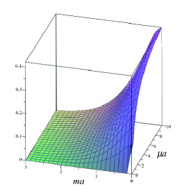
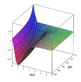
where we have a Coulombian behavior modulated by the expression inside brackets. The correction due to the Lorentz symmetry breaking is given by the functions ${\cal F}_{p}$ and ${\cal F}_{3}$, the first one is associated with the components of the background vector parallel to the mirror and the second one, with the component perpendicular to the mirror. ${\cal F}_{p}$ is positive in its domain and ${\cal F}_{3}$ assume positive and negative values, as shown in Fig. 1 and 2. Both functions vanish in the limit $\mu=0$, where we have no mirror present.

Figure 1: Function ${\cal F}_{p}$, appearing in the force described in Eq. (88), where the vertical axis is in arbitrary units.

Figure 2: Function ${\cal F}_{3}$, appearing in the force described in Eq. (88), where the vertical axis is in arbitrary units.

The second phenomena is obtained when we fix the distance between the charge and the mirror and vary the orientation of the whole system with respect to the background vector. In this case, we can show that a torque emerges on the system. In order to calculate this torque, we define as $0\leq\alpha\leq\pi$ the angle between the normal to the mirror ($\hat{x}^{3}$) and the background vector, in such a way that

$$(v^{3})^{2}={\bf v}^{2}\cos^{2}(\alpha)\ \ ,\ \ {\bf{v}}_{p}^{2}={\bf v}^{2}\sin^{2}(\alpha)\ ,$$ (89)

then the torque can be computed from Eq. (83) as follows,

$$\tau_{MC}=-\frac{\partial E_{MC}}{\partial\alpha}=-\frac{\mu\sigma^{2}{\bf v}^{2}}{16\pi}\sin(2\alpha)\left[\left(\mu a+\frac{1}{2}\right)e^{\mu a}Ei\left(1,2ma+\mu a\right)-\frac{(m+\mu)}{(2m+\mu)}e^{-2ma}\right]\thinspace.$$ (90)

Equation (90) is a new effect, which disappears in the $v=0$ limit. Defining the function

$${\cal T}(x,y)=x\left[\frac{(y+x)}{(2y+x)}e^{-2y}-\left(x+\frac{1}{2}\right)e^{x}Ei\left(1,2y+x\right)\right]\thinspace,$$ (91)

we can write Eq. (90) in the form

$$\tau_{MC}=\frac{\sigma^{2}{\bf v}^{2}}{16\pi}\frac{1}{a}\sin(2\alpha){\cal T}(\mu a,ma)\ .$$ (92)

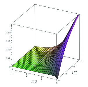
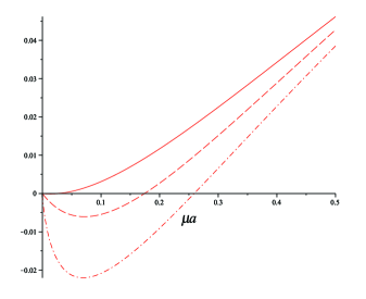
In Fig. (3), we show the behavior of ${\cal T}$ in terms of $\mu a$ and $ma$. The function is positive except in a very small region around $\mu a=ma=0$, and goes to zero if $ma$ is large or $\mu a$ approaches zero. This behavior can also be seen in Fig. (4), where we have three plots, with three different values for the mass, in the vicinity of $\mu a=0$. In the limit $\mu a\to 0$, the result in Eq. (91) vanishes, as expected. This torque and the force modulation contained in Eq. (88) are phenomenological signatures of the Lorentz violation introduced by the $v^{\mu}$, and might be relevant in experimental setups involving mirrors.

Figure 3: Function ${\cal T}$ of Eq. (91), where the vertical axis is in arbitrary units.

Figure 4: Graph of the function ${\cal T}$ for $ma=0$ (dash-point), $ma=0.1$ (dash) and $ma=0.2$ (solid) as a function of $\mu a$, where the vertical axis is in arbitrary units.

For the massless case, the energy (83) becomes

$$E_{MC}\left(m=0\right)=\frac{\mu\sigma^{2}}{16\pi}\Biggl{\{}e^{\mu a}Ei\left(1,\mu a\right)+\frac{{\bf{v}}_{p}^{2}}{2}e^{\mu a}Ei\left(1,\mu a\right)+(v^{3})^{2}\left[\left(\mu a+1\right)e^{\mu a}Ei\left(1,\mu a\right)-1\right]\Biggr{\}}\ .$$ (93)

The limit $\mu\rightarrow\infty$ is interesting, corresponding physically to the field subjected to Dirichlet boundary conditions in the plane. In this limit, we have a perfect two-dimensional mirror and, from Eq. (83), we obtain

$$E_{MC}\left(\mu\rightarrow\infty\right)=\frac{\sigma^{2}}{16\pi}\frac{e^{-2ma}}{a}\left(1+\frac{{\bf{v}}_{p}^{2}}{2}-ma(v^{3})^{2}\right)\ .$$ (94)

The first term on the right hand side is the three-dimensional Yukawa potential between two charges at a distance $2a$ apart. The second and third terms are corrections due to the Lorentz symmetry breaking up to second order in $v^{\mu}$. The corresponding interaction force between the point-like charge and the perfect mirror is given by

$$F_{MC}\left(\mu\rightarrow\infty\right)=-\frac{\partial E_{MC}\left(\mu\rightarrow\infty\right)}{\partial a}=\frac{\sigma^{2}}{8\pi}\frac{e^{-2ma}}{a}\left[\left(1+\frac{{\bf{v}}_{p}^{2}}{2}\right)\left(m+\frac{1}{2a}\right)-m^{2}a(v^{3})^{2}\right]\thinspace.$$ (95)

In Eq. (40) we have the interaction force between two point-like scalar charges for the model (1). Expanding this expression up to second order in $v^{\mu}$, we can obtain the interaction force for the special case where we have two opposite point-like charges, $\sigma_{1}=\sigma$ and $\sigma_{2}=-\sigma$, placed at a distance $2a$ apart. In this specific situation, this force turns out to be equivalent to Eq. (95). The interesting conclusion is that the image method is valid for the Lorentz violation theory (1) up to second order in $v^{\mu}$ for the Dirichlet boundary condition.

Taking the limit when $\mu\rightarrow\infty$ in Eq. (93) or equivalently putting $m=0$ in (94), we obtain the interaction energy between a point charge and a perfect mirror for the massless scalar field, and consequently the interaction force,

$$F_{MC}\left(\mu\rightarrow\infty,m=0\right)=\frac{\sigma^{2}}{16\pi a^{2}}\left(1+\frac{{\bf{v}}_{p}^{2}}{2}\right)\ ,$$ (96)

which is the usual Coulombian force with an overall minus sign between the scalar charge and its image, placed at a distance $2a$ apart. With the same analysis, one can argue that Eq. (96) is in agreement with Eq. (42), and again the validity of the image method is verified. In the same limit, from Eq. (90), we have

$$\tau_{MC}\left(\mu\rightarrow\infty,m=0\right)=-\frac{\partial E_{MC}\left(\mu\rightarrow\infty,m=0\right)}{\partial\alpha}=\frac{\sigma^{2}{\bf{v}}^{2}}{32\pi a}\sin(2\alpha)\ .$$ (97)

When $\alpha=0,\pi/2,\pi$, corresponding to the mirror being parallel, perpendicular or antiparallel to the background vector ${\bf v}$, the torque (97) vanishes. The configurations $\alpha=0,\pi$ are stable equilibrium situations, while for $\alpha=\pi/2$ we have an unstable equilibrium point. When $\alpha=\pi/4,3\pi/4$, the torque (97) exhibits its maximum and minimum values, respectively. The equilibrium situation is attained when the mirror is parallel or antiparallel to the background vector.

IV.2 Exact results

The first case in which we can provide exact results is when $v^{\mu}=v_{p}^{\mu}$, what leads to

$$E_{MC}=\frac{\mu\sigma^{2}}{8\pi^{2}}\int d^{2}{\bf{p}}_{p}\frac{e^{-2a\sqrt{{\bf{p}}_{p}^{2}-\left({\bf{p}}_{p}\cdot{\bf{v}}_{p}\right)^{2}+m^{2}}}}{2\sqrt{{\bf{p}}_{p}^{2}-\left({\bf{p}}_{p}\cdot{\bf{v}}_{p}\right)^{2}+m^{2}}\left(2\sqrt{{\bf{p}}_{p}^{2}-\left({\bf{p}}_{p}\cdot{\bf{v}}_{p}\right)^{2}+m^{2}}+\mu\right)}\ .$$ (98)

Performing a change in the integration variables similar to the one we have made in the Appendix, and then using polar coordinates, we have

$$E_{MC}=\frac{\mu\sigma^{2}}{4\pi\sqrt{1-{\bf{v}}_{p}^{2}}}\int_{0}^{\infty}dq\ q\frac{e^{-2a\sqrt{q^{2}+m^{2}}}}{2\sqrt{q^{2}+m^{2}}\left(2\sqrt{q^{2}+m^{2}}+\mu\right)}\ .$$ (99)

Now, carrying out the change of integration variable $y=2\sqrt{q^{2}+m^{2}}$, we obtain

$$E_{MC}=\frac{\mu\sigma^{2}}{16\pi\sqrt{1-{\bf{v}}_{p}^{2}}}e^{\mu a}Ei\left(1,2ma+\mu a\right)\ .$$ (100)

Equation (100) gives the exact expression for the interaction energy between a point-like current and a semi-transparent mirror for the special case where the background vector has only the parallel components to the mirror. We notice that (100) is the usual result found in standard scalar field theory with an effective coupling constant $\sigma\rightarrow\sigma\left(1-{\bf{v}}_{p}^{2}\right)^{-1/4}$. Taking the limit $\mu\rightarrow\infty$ in Eq. (100) and computing the interaction force, we arrive at

$$F_{MC}\left(\mu\rightarrow\infty\right)=\frac{\sigma^{2}}{16\pi\sqrt{1-{\bf{v}}_{p}^{2}}}\frac{e^{-2ma}}{a}\left(2m+\frac{1}{a}\right)\ ,$$ (101)

which is the interaction force characterized by the Dirichlet’s boundary condition.

In Eq. (40) we have the exact interaction force between two point-like currents. For the special situation where $v^{3}=0,\sigma_{1}=\sigma,\sigma_{2}=-\sigma$ and $a\to 2a$, this result turns out to be equivalent to Eq. (101). Thus, we again verify that for this special case, $(v^{3}=0)$, the image method is valid.

The second exact case we discuss is when only $v^{3}$ is nonzero, what leads to the result

$$E_{MC}=\frac{\sigma^{2}}{16\pi}\frac{\mu}{\left[1-(v^{3})^{2}\right]}e^{\mu a\left[1-(v^{3})^{2}\right]^{-1}}Ei\left(1,2ma\left[1-(v^{3})^{2}\right]^{-1}+\mu a\left[1-(v^{3})^{2}\right]^{-1}\right)\ .$$ (102)

Eq. (102) is equivalent to the result obtained in standard scalar field theory with an effective mass $m\rightarrow m\left[1-(v^{3})^{2}\right]^{-1}$ and an effective degree of transparency of the mirror $\mu\rightarrow\mu\left[1-(v^{3})^{2}\right]^{-1}$. From Eq. (102) we can compute the interaction force in the limit $\mu\rightarrow\infty$, resulting in

$$F_{MC}\left(\mu\rightarrow\infty\right)=\frac{\sigma^{2}}{16\pi}\frac{e^{-2m\left[1-(v^{3})^{2}\right]^{-1}a}}{a}\left(\frac{1}{a}+2m\left[1-(v^{3})^{2}\right]^{-1}\right)\ .$$ (103)

For the massless case, the interaction force (103) becomes the corresponding Coulombian interaction between two charges at a distance $2a$ apart with an overall minus sign. Thus, in this particular scenario, Lorentz violation effects disappear from the end result. As before, taking ${\bf{v}}_{p}^{\mu}=0,\sigma_{1}=\sigma,\sigma_{2}=-\sigma$ and $a\to 2a$ in Eq. (40), we reproduce the result in Eq. (103). Thus, the image method is also valid for the case where $v^{\mu}=\left(0,0,0,v^{3}\right)$.

It is important to mention that the validity of the image method in a Lorentz-violating scenario is a non-trivial result, since the presence of the LV background reduces the symmetry of the problem, which is a key element in the application of the method. This suggests that the presence of mirrors in Lorentz-violating scenarios is a subject which deserves more investigation.

V Final Remarks

In this paper, we investigated the interactions between external sources for a massive real scalar field in the presence of an aether-like CPT-even Lorentz symmetry breaking term. First we performed an analysis in $D_{\perp}+D+1$ dimensions where we considered steady field sources concentrated along parallel $D$-branes, without recourse to any approximation schemes. We discussed some particular instances of our general results and observed effects with no counterpart in the standard (Lorentz invariant) scalar field theory. For example, we have shown the emergence of an spontaneous torque on a classical scalar dipole which is an exclusive effect due to the Lorentz symmetry breaking, agreeing with results obtained in different, more complicated models such as borges1 .

Afterwards, some consequences of the Lorentz violation theory (1) due to the presence of a semi-transparent mirror were studied in $3+1$ dimensions. We considered different configurations of the background vector, starting by taking into account all the components of the background vector, and treating it perturbatively up to second order. Next, we provided exact results for two special cases, specifically when the background vector has only components parallel and perpendicular to the mirror. For all these configurations of the background vector, we obtained the propagator for the scalar field and the interaction force between the mirror and a point-like current. We showed that the image method is valid in the considered theory for Dirichlet boundary condition. We also showed that a new effect arises from the obtained results, a torque acting on the mirror according to its positioning with respect to the background vector.

These results suggest that the extension of these studies to more general LV models is a very interesting prospect. Despite not being directly applicable to the phenomenological search of Lorentz violation established within the formalism of the Standard Model extensionSME1 ; SME2 ; SME3 ; SME4 , the scalar field can still be explored as a prototype, establishing interesting effects of LV yet to be explored. A first natural extension of our results would be to more general LV backgrounds as described by Eq. (2). The extension of these studies for non-minimal (higher-derivative) LV models would also be of interest.

Acknowledgments. The authors would like to thank V. A. Kostelecky for reading the manuscript and providing important feedback. This work was partially supported by Conselho Nacional de Desenvolvimento Científico e Tecnológico (CNPq) and Fundação de Amparo à Pesquisa do Estado de São Paulo (FAPESP), via the following grants: CNPq 311514/2015-4, CNPq 313978/2018-2 (FAB), CNPq 304134/2017-1 and FAPESP 2017/13767-9 (AFF), FAPESP 2016/11137-5 (L.H.C.B.).

Appendix A The Eqs. (71) and (73)

In this appendix we provide additional details on the computation of Eqs. (71) and (73). We note that in some of the intermediate expressions that follow, the condition $v^{2}=0$ cannot be imposed to ensure the tracelessness of the LV coefficient $k^{\mu\nu}$ defined in Eq. (2); however, this condition can be safely imposed in the final result, from which one can obtain, in the proper limiting cases, the perturbative results previously obtained, thus ensuring the consistency of the calculation.

Starting from Eq. (4), in order to put $G_{0}\left(x,y\right)$ in an appropriated form, we have to carry out a change of the integration variables similar to the ones employed in references LHCFAB1 ; scalar3 . We split the four-vector momentum $p^{\mu}$ into two parts, one parallel, ${p}_{pa}^{\mu}$, and the other normal, ${p}_{no}^{\mu}$, to the Lorentz violation parameter $v^{\mu}$,

$${p}^{\mu}={p}_{no}^{\mu}+{p}_{pa}^{\mu}\ ,\ {p}=\Bigl{(}\frac{{v}\cdot{p}}{{v}^{2}}\Bigr{)}{v^{\mu}}\ ,\ {p}_{no}^{\mu}={p}^{\mu}-\Bigl{(}\frac{{v}\cdot{p}}{{v}^{2}}\Bigr{)}{v^{\mu}}\ ,$$ (104)

where ${p}_{no}\cdot{v}=0$ and $\left(p\cdot v\right)^{2}=p_{pa}^{2}v^{2}$ . Now, we define the four-vector ${q^{\mu}}$

$${q}^{\mu}={p}_{no}^{\mu}+{p}_{pa}^{\mu}\sqrt{1+{v}^{2}}={p}^{\mu}+\Bigl{(}\frac{{v}\cdot{p}}{{v}^{2}}\Bigr{)}(\sqrt{1+{v}^{2}}-1)v^{\mu}\ .$$ (105)

With definitions (104) and (105), we have

$${p}_{pa}^{\mu}=\frac{(v\cdot q)}{{v}^{2}}\frac{v^{\mu}}{\sqrt{1+{v}^{2}}}\ \ \ ,\ \ \ {p}_{no}^{\mu}=q^{\mu}-\frac{(v\cdot q)}{{v}^{2}}v^{\mu}\thinspace,$$ (106)

$${p}^{\mu}={q}^{\mu}+\frac{(v\cdot q)}{{v}^{2}}\left(\frac{1}{\sqrt{1+{v}^{2}}}-1\right)v^{\mu}\ ,$$

and

$${q}^{2}={p}^{2}+({p}\cdot{v})^{2}\thinspace.$$ (107)

With the aid of the definition

$${b}^{\mu}=\left({x^{\mu}-y^{\mu}}\right)+\left(\frac{1-\sqrt{1+{v}^{2}}}{\sqrt{1+{v}^{2}}}\right)\left(\frac{{v}\cdot\left({x-y}\right)}{{v}^{2}}\right)v^{\mu}\ ,$$ (108)

and Eq. (106), we obtain

$${p}\cdot{\left(x-y\right)}={b}\cdot{q}$$ (109)

The Jacobian of the transformation from ${p}^{\mu}$ to ${q}^{\mu}$ can be calculated from Eq. (106)

$$\det\left[\frac{\partial{p}^{\mu}}{\partial{q}_{\nu}}\right]=-\frac{1}{\sqrt{1+{v}^{2}}}\ .$$ (110)

Using these results, we obtain

$$G_{0}\left(x,y\right) =-\frac{1}{\sqrt{1+{v}^{2}}}\int\frac{d^{4}q}{\left(2\pi\right)^{4}}\frac{e^{ib\cdot q}}{(q^{2}-m^{2})}$$

$$=-\frac{1}{\sqrt{1+{v}^{2}}}\int\frac{d^{3}q_{p}}{\left(2\pi\right)^{3}}\ e^{ib_{p}\cdot q_{p}}\int\frac{dq^{3}}{2\pi}\frac{e^{-iq^{3}b^{3}}}{(q^{2}-m^{2})}\ .$$ (111)

The first integral in Eq. (111) is given by

$$\int\frac{d^{3}q_{p}}{\left(2\pi\right)^{3}}\ e^{ib_{p}\cdot q_{p}}=-\sqrt{1+v_{p}^{2}}\int\frac{d^{3}p_{p}}{\left(2\pi\right)^{3}}\ e^{ip_{p}\cdot\left(x_{p}-y_{p}\right)}\ ,$$ (112)

where we used the Eqs. (109) and (110), while the last integral is given by

$$\int\frac{dq^{3}}{2\pi}\frac{e^{-iq^{3}b^{3}}}{(q^{2}-m^{2})}=-\frac{e^{-L\mid b^{3}\mid}}{2L}\ ,$$ (113)

where $L=\sqrt{m^{2}-q_{p}^{2}}$ or, from Eq. (107), $L=\sqrt{m^{2}-\left[p_{p}^{2}+\left(p_{p}\cdot v_{p}\right)^{2}\right]}$, and $b^{3}$ is found by taking $\mu=3$ in (108), as follows,

$$b^{3}=\left(x^{3}-y^{3}\right)+\left(\frac{1-\sqrt{1+{v}^{2}}}{\sqrt{1+{v}^{2}}}\right)\left(\frac{{v}\cdot\left({x-y}\right)}{{v}^{2}}\right)v^{3}\ ,$$ (114)

Collecting terms, we write

$$G_{0}\left(x,y\right)=\int\frac{d^{3}p_{p}}{\left(2\pi\right)^{3}}\ e^{ip_{p}\cdot\left(x_{p}-y_{p}\right)}\left[-\frac{1}{2}\ \sqrt{\frac{1+v_{p}^{2}}{1+v^{2}}}\frac{e^{-L\mid b^{3}\mid}}{L}\right]\ .$$ (115)

Finally, taking $v^{3}=0$ in the term between brackets on the right-hand side of the Eq. (115), we obtain the Eq. (71). In the same way, taking $v_{p}^{\mu}=0$ , we obtain Eq. (73).

References

- (1) D. Colladay and V. A. Kostelecky, Phys. Rev. D 55, 6760 (1997).
- (2) D. Colladay and V. A. Kostelecky, Phys. Rev. D 58, 116002 (1998).
- (3) S. Coleman and S. L. Glashow, Phys. Lett. B 405, 249 (1997).
- (4) S. Coleman and S. L. Glashow, Phys. Rev. D 59, 116008 (1999).
- (5) G. P. de Brito, J. T. Guaitolini Junior, D. Kroff, P. C. Malta and C. Marques, Phys. Rev. D 94, 056005 (2016).
- (6) D. Colladay, V. A. Kostelecky, Phys. Lett. B 511, 209 (2001).
- (7) M. A. Hohensee, R. Lehnert, D. F. Phillips, R.L. Walsworth, Phys. Rev. D 80, 036010 (2009).
- (8) A. A. Andrianov, R. Soldati, L. Sorbo, Phys. Rev. D 59, 025002 (1998).
- (9) A. A. Andrianov, P. Giacconi, R. Soldati, J. High Energy Phys. 02, 030 (2002).
- (10) F. R. Klinkhamer, M. Schreck, Nucl. Phys. B 848, 90 (2011).
- (11) A.J.G.Carvalhoa, A.F.Ferrari, A.M.de Lima, J.R.Nascimento and A.Yu.Petrov 942, 393 (2019).
- (12) T. Mariz, R.V. Maluf, J.R. Nascimento and A. Yu. Petrov, Int. J. Mod. Phys. 33, 1850018 (2018).
- (13) T. Mariz, J.R. Nascimento and E. Passos, Braz. J. Phys. 36, 1171 (2006).
- (14) J. R. Nascimento, E. Passos, A. Yu. Petrov, and F. A. Brito, J. High Energy Phys. 0706, 016 (2007).
- (15) O. M. Del Cima, J. M. Fonseca, D. H. T. Franco, and O. Piguet, Phys. Lett. B 688, 258 (2010).
- (16) J. M. Chung and B. K. Chung, Phys. Rev. D 63, 105015 (2001).
- (17) L. H. C. Borges and F. A. Barone, Eur. Phys. J. C 693, 77 (2017).
- (18) L. H. C. Borges, F. A. Barone, J. A. Helayël-Neto, Eur. Phys. J. C 74, 2937 (2014).
- (19) R. Casana, M. M. Ferreira Jr., C. E. H. Santos, Phys. Rev. D 78, 105014 (2008).
- (20) R. Casana, M. M. Ferreira Jr., A. R. Gomes, P. R. D. Pinheiro, Eur. Phys. J. C 62, 573 (2009).
- (21) Q. G. Bailey, V. A. Kostelecky, Phys. Rev. D 70, 076006 (2004).
- (22) L.H.C. Borges and F.A. Barone, Braz. J. Phys. 49, 571 (2019).
- (23) H. Belich Jr., M.M. Ferreira Jr., J.A. Helayël-Neto and M.T.D. Orlando, Phys. Rev. D 68, 025005 (2003).
- (24) R. Casana, M.M. Ferreira Jr. and R.P.M. Moreira, Eur. Phys. J. C 72, 2070 (2012)
- (25) M.B. Cruz, E.R. Bezerra de Mello and A.Yu. Petrov, Phys. Rev. D 99, 085012 (2019).
- (26) A. Mojavezia, R. Moazzemib, M.E. Zomorrodian, Nucl. Phys. B 941 145 (2019).
- (27) M. Frank and I. Turan, Phys. Rev. D 74, 033016 (2006).
- (28) L.H.C. Borges and F.A. Barone, Eur. Phys. J. C 76, 64 (2016).
- (29) L.H.C. Borges, F.A. Barone and A.F. Ferrari, Europhys. Lett. 122, 31002 (2018).
- (30) R. Casana, M.M. Ferreira Jr., L. Lisboa-Santos, F.E.P. dos Santos and Marco Schreck, Phys. Rev. D 97, 115043 (2018).
- (31) F.E.P. dos Santos and M.M. Ferreira Jr., Symm. 10, 302 (2018).
- (32) Manoel M. Ferreira Jr., L. Lisboa-Santos, R.V. Maluf and Marco Schreck, [arXiv:1903.12507] (2019).
- (33) T. Mariz, J.R. Nascimento, A.Yu. Petrov, and C.M. Reyes, Phys. Rev. D 99, 096012 (2019).
- (34) J.R. Nascimento, A. Yu. Petrov and C.M. Reyes, J. Phys.: Conf. Ser. 952, 012017 (2018).
- (35) J.R. Nascimento1, A.Yu.Petrov and C.M. Reyes, Eur. Phys. J. C 78, 541 (2018).
- (36) M. S. Berger and V. A. Kostelecky, Phys. Rev. D 65, 091701(R) (2002).
- (37) M.N. Barreto, D. Bazeia, and R. Menezes, Phys. Rev. D 73, 065015 (2006).
- (38) B. Altschul, Phys. Lett. B 639, 679 (2006).
- (39) A. Ferrero and B. Altschul, Phys. Rev. D 84, 065030 (2011).
- (40) P.R.S. Carvalho, Phys. Lett. B 726, 850 (2013); Phys. Lett. B 730, 320 (2014).
- (41) B. Altschul, Phys. Rev. D 87, 045012 (2013).
- (42) R. Casana and K.A.T. da Silva, Mod. Phys. Lett. A 30, 1550037 (2015).
- (43) A.P. Baeta Scarpelli, L.C.T. Brito, J.C.C. Felipe, J.R. Nascimento, and A.Yu. Petrov, Eur. Phys. J. C 77, 850 (2017).
- (44) Z. Xiao, Phys. Rev. D 98, 035018 (2018).
- (45) T. de Paula Netto, Phys. Rev. D 97, 055048 (2018).
- (46) G.S. Silva and P.R.S. Carvalho, Int. J. Geom. Meth. Mod. Phys. 15, 1850086 (2018).
- (47) B. R. Edwards and V. A. Kostelecky, Phys. Lett. B 786, 319 (2018).
- (48) D.L. Anderson, M. Sher and I. Turan, Phys. Rev. D 70 016001 (2004).
- (49) R. Kamand, B. Altschul, and M.R. Schindler, Phys. Rev. D 95, 056005 (2017).
- (50) M. B. Cruz, E. R. Bezerra de Mello and A. Yu. Petrov, Phys. Rev. D 96, 045019 (2017).
- (51) M. B. Cruz, E. R. Bezerra de Mello and A. Yu. Petrov, Mod. Phys. Lett. A 33, 1850115 (2018).
- (52) V. A. Kostelecky, Phys. Rev. D 69, 105009 (2004) .
- (53) V. A. Kostelecky, J. D. Tasson, Phys. Rev. D, 83 016013 (2011).
- (54) F. A. Barone and G. Flores-Hidalgo, Phys. Rev. D 78, 125003 (2008).
- (55) F. A. Barone and G. Flores-Hidalgo, Braz. J. Phys. 40, 188 (2010).
- (56) G. B. Arfken and H. J. Weber, Mathematical Methods for Physicists, Academic Press (1995).
- (57) L. H. C. Borges, A. F. Ferrari and F. A. Barone, Eur. Phys. J. C 76, 599 (2016).
- (58) C. G. Shao, Y. J. Tan, W. H. Tan, S. Q. Yang, J. Luo and M. E. Tobar, Phys. Rev. D 91, 102007 (2015).
- (59) G. T. Camilo, F. A. Barone and F. E. Barone, Phys. Rev. D 87, 025011 (2013).
- (60) R. M. Cavalcanti, [arXiv:hep-th/0201150].
- (61) F.A. Barone and F.E. Barone, Phys. Rev. D 89, 065020 (2014).
- (62) F.A. Barone and F.E. Barone, Eur. Phys. J. C 74, 3113 (2014).
- (63) I.S. Gradshteyn and I.M. Ryzhik, Table of Integrals, Series, and Products, Academic Press (2000).