Unusual scaling in a discrete quantum walk with random long range steps

Abstract

A discrete time quantum walker is considered in one dimension, where at each step, the translation can be more than one unit length chosen randomly. In the simplest case, the probability that the distance travelled is $\ell$ is taken as $P(\ell)=\alpha\delta(\ell-1)+(1-\alpha)\delta(\ell-2^{n})$ with $n\geq 1$. Even the $n=1$ case shows a drastic change in the scaling behaviour for any $\alpha\neq 0,1$. Specifically, $\langle x^{2}\rangle\propto t^{3/2}$ for $0<\alpha<1$, implying the walk is slower compared to the usual quantum walk. This scaling behaviour, which is neither conventional quantum nor classical, can be justified using a simple form for the probability density. The decoherence effect is characterized by two parameters which vanish in a power law manner close to $\alpha=0$ and $1$ with an exponent $\approx 0.5$. It is also shown that randomness is the essential ingredient for the decoherence effect.

1 Introduction

Discrete time quantum walk (DTQW) is a phenomenon in which a random walker has a coin (also called chiral) degree of freedom which dictates the translational motion of the walker at each discrete time step [1, 2, 3, 4, 5, 6]. In contrast to the classical case, the walk may propagate in different directions simultaneously as the walker may exist in a superposition of coin states. The time dependence of the square of the displacement for a quantum walk is $\langle x^{2}\rangle\propto t^{2}$ showing it is much faster than the classical walker (where $\langle x^{2}\rangle\propto t$), and hence can play a key role in many dynamical processes. Apart from the discrete walk, the continuous time quantum walk has also been conceived [7] where the coin degree of freedom is not present. The speeding up over classical walk is noted in both discrete and continuous walks.

The quantum walk can be slowed down by decoherence effects [8]; in most cases this leads to a transition to a classical diffusive walk. Decoherence and subsequent localisation can take place due to several factors like randomness in the environment, defects in the embedding lattice or graphs, measurements of the position or chirality of the walk, inertia, etc. Decoherence has been studied in one dimensional [9, 10, 11, 12, 13, 14, 15, 16, 17, 18, 19, 20, 21, 22] and two dimensional [22, 23, 24, 25, 26, 27] discrete walks as well as in the continuous quantum walk [28, 29, 30]. Such noisy quantum walks can even be non-unitary [8, 31]. Experimentally, cases with both static and dynamic disorder have been studied [32] resulting in Anderson localization type phenomena and diffusive behaviour respectively. In the cases studied so far, the results are strongly dependent on the parameters controlling the decoherence.

In most of the earlier works in one dimension, the disorder has been incorporated through the coin operator in different ways. In certain cases, stochasticity in position space has also been considered, for example, by breaking links. In this work, we consider a discrete time quantum walk on a line with dynamic disorder in the translational motion.

Usually, it is assumed that the translation of the quantum walker is of equal length at each time step. We relax this condition by allowing the translation through a distance $\ell\geq 1$, chosen randomly, at each time step. Such long range hopping has been considered in quantum transport phenomena by including interaction with a thermal bath of oscillators in a tight binding model [33] to study decoherence effects. While the longer steps can make the transport faster, the randomness will also have its effect by slowing it down. In this paper, we intend to investigate the result of this competition in the quantum walk on a line. The probability distribution of the position of the quantum walker and its moments are calculated and the primary objective in the present paper is to compare the behaviour of these quantities with the conventional classical random and non-random quantum walks.

In section 2 we describe the quantum walk considered in the paper and the details of the quantities calculated. The results are presented and analysed in section 3. A concluding section is added in the end.

2 The random long ranged walk

In the quantum walk in one dimension, the state of the walker is expressed in the $|x\rangle\otimes|d\rangle$ basis, where $|x\rangle$ is the position (in real space) eigenstate and $|d\rangle$ is the chirality eigenstate (either left ($|L\rangle$) or right ($|R\rangle$)). The state of the particle, $\psi({x},t)$ can be written as

$$\psi({x},t)=\left[{\begin{array}[]{cc}\psi_{L}({x},t)\\ \psi_{R}({x},t)\end{array}}\right]$$ (1)

For the rotation in the chiral space, we have used the Hadamard coin [4, 5] unitary operator $H$ represented by

$$H=\frac{1}{\sqrt{2}}\left[{\begin{array}[]{cc}1&1\\ 1&-1\end{array}}\right]$$ (2)

The occupation probability of site $x$ at time $t$ is given by $f(x,t)=|\psi_{L}({x},t)|^{2}+|\psi_{R}({x},t)|^{2}$ ; sum of these probabilities over all $x$ is $1$ at each time step. The walk is initialized at the origin with $\psi_{L}(0,0)=a_{0},\psi_{R}(0,0)=b_{0};~{}~{}a_{0}^{2}+b_{0}^{2}=1$ and $\psi_{L}(x\neq 0,t=0)=\psi_{R}(x\neq 0,t=0)=0$.

As long as the displacement $\ell$ at each step is a constant, results are independent of $\ell$ apart from a trivial scaling factor. In the present case, the value of $\ell$ is chosen randomly from a distribution. The conditional translation operator at any time $t$ can then be written in a compact form:

$$T(t)=|R\rangle\langle R|\otimes\sum_{x}|x+\ell(t)\rangle\langle x|+|L\rangle\langle L|\otimes\sum_{x}|x-\ell(t)\rangle\langle x|.$$

The distribution of $\ell$ can be chosen in many ways, we choose one which introduces longer step lengths in the simplest possible manner. We consider only two possible step lengths: $\ell=1$ and $\ell=l_{max}=2^{n}$ with $n\geq 1$ ($n$ having a fixed value) and

$$P(\ell)=\alpha\delta(\ell-1)+(1-\alpha)\delta(\ell-2^{n}).$$ (3)

The limits $\alpha=1$ and $\alpha=0$ are equivalent to usual quantum walks and it is sufficient to consider the interval $0.5\leq\alpha<1.0$ due to symmetry; $\alpha=0.5$ is the case with maximum randomness and $\alpha=1$ corresponds to zero randomness. Note that in a classical walk one can also introduce such a variation, for finite values of $n$, the scaling of the moments will remain the same due to central limit theorem.

The walk is initialised with $a_{0}=\sqrt{\frac{1}{3}}$ and $b_{0}=\sqrt{\frac{2}{3}}$ such that in absence of disorder, an asymmetric probability density profile is obtained and one can study the scaling of both the first and second moments. The results are averaged over 1000 configurations.

We have evaluated $f(x,t)$ for the long ranged walk and studied the scaling behaviour of the first two moments. In the present work, only one parameter controlling the randomness has been used.

3 Results and analysis

3.1 Results for $n=1$

We first consider the case where step lengths are either 1 or 2 chosen according to eq. (3). We note that as soon as $\alpha$ deviates from unity, the shape of $f(x,t)$ assumes a completely different form. $f(x,t)$ shows two ballistic peaks and an additional peak around zero, the latter is absent for the quantum walker. It may be mentioned that this shape is not a result of averaging over different realisations, even a single configuration shows these features. Fig. 1 shows the distributions for $n=1$ with $\alpha=0.5$ and $\alpha=0.995$. The result for $\alpha=1$ (i.e., $l_{max}=1$, the usual case), is also shown for comparison. We also note that while asymmetry is maintained in the ballistic peaks, the centrally peaked part is symmetric. As $\alpha$ is increased from 0.5, the width of the distribution decreases as more steps with $\ell=1$ is taken compared to $\ell=2$. Although the range is almost same for $\alpha=1$ and $\alpha=0.995$, even the small deviation of $\alpha$ from unity is effective in making the distribution strikingly different from that at $\alpha=1$. As $\alpha$ approaches $1$, the peak value of $f(x,t)$ at $x=0$ becomes less compared to the ballistic peaks in height.

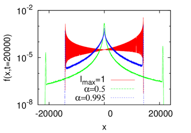
Figure 1: $f(x,t)$ for the quantum long ranged walk with step sizes 1 and 2 with probability $\alpha$ and $(1-\alpha)$ respectively. Results for $\alpha=0.995$ and $0.5$ are compared with the case $\alpha=1$ where the maximum step size $l_{max}=1$.

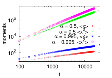
Figure 2: The first two moments of $f(x,t)$ for two extreme values of $\alpha$ are shown ($n=1$). The continuous lines are best fit curves obtained using the the form given in Equations 5 and 6.

Plotting the first two moments, $\langle x\rangle$ and $\langle x^{2}\rangle$, we note a drastic change in the scaling forms compared to $\alpha=1$. For any value of $\alpha\neq 1$, the asymptotic behaviour suggests $\langle x\rangle\propto t^{1/2}$ and $\langle x^{2}\rangle\propto t^{3/2}$ shown in Fig. 2. The scaling of the fluctuations $\langle x^{2}\rangle-\langle x\rangle^{2}$ follows the same scaling form as $\langle x^{2}\rangle$. This indicates that the quantum walker, when allowed to take long range steps randomly, ends up being slower than usual.

We also note that the two ballistic peaks of $f(x,t)$ occur approximately at $x=\pm(2-\alpha)t/\sqrt{2}$ which corresponds to a simple weighted linear superposition of the two cases for $\ell=1$ and $\ell=2$ for the usual DTQW. Hence the range decreases linearly with $\alpha$ which is to be expected. However, although $\langle x^{2}\rangle\propto t^{3/2}$ for all $\alpha<1$, the actual value of $\langle x^{2}\rangle$ varies non-monotonically with $\alpha$ (see Fig. 3); as $\alpha$ is increased from 0.5, it first shows a decrease but then increases beyond $\alpha\approx 0.8$. This indicates the walker is localised maximally for a value of $\alpha\simeq 0.8$ and not at $0.5$ as one would naively expect. We will get back to this point later.

Analysing the probability densities, one finds that $f(x,t)$ shows two distinct scaling behaviour: plotting $t^{\gamma}f(x,t)$ against the scaled variable $x/t^{\gamma}$, the central part collapses with $\gamma=0.5$, while with $\gamma=1$ the extreme values show a collapse; this happens for all values of $\alpha\neq 1$; data for two extreme values are shown in Fig. 4.

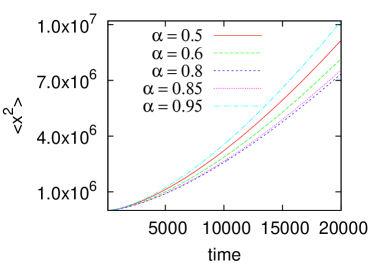
Figure 3: The second moment of the distribution $f(x,t)$ shown against time for different values of $\alpha$ (n=1). It shows a minimum value at $\alpha\simeq 0.8$.

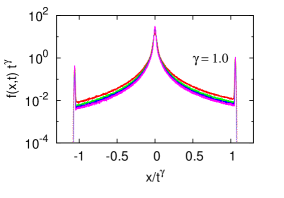
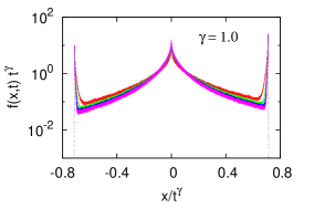
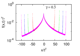
Figure 4: Data collapse of $f(x,t)$ for four different values of $t$ for the ballistic peaks and the central peak for $\alpha=0.5$ (top panel) and $\alpha=0.995$ (bottom panel). All data are for $n=1$.

In order to obtain an approximate estimate of the moments, the problem one faces is that no simple form of the distributions exists. Still, one can make a rather gross approximation by taking $f(x,t)$ (for $\alpha\neq 1$) to be a discrete function with non-zero values at three points only: $x=0$ (where the central peak occurs) and $x=\pm ct$ (where the ballistic peaks occur). Noting the peak values scale as $1/\sqrt{t}$ and $1/t$ at these three points, one can write $f(x,t)$ as

$$f(x,t)=a_{1}\frac{1}{t}\delta(x-ct)+a_{2}\frac{1}{t}\delta(x+ct)+a_{3}\frac{1}{\sqrt{t}}\delta(x).$$ (4)

In general, $a_{1}\neq a_{2}$ as the walk is asymmetric. From Eq. (4), one can estimate the first two moments as

$$\langle x\rangle=t/(b_{1}+{b_{2}}\sqrt{t})$$ (5)

and

$$\langle x^{2}\rangle=t^{2}/(b_{3}+b_{4}\sqrt{t}),$$ (6)

where $b_{i}$ are related to the constants $a_{i}$ and $c$.

The above forms of $\langle x\rangle$ and $\langle x^{2}\rangle$ are consistent with their asymptotic bahaviour obtained numerically. More importantly, fitting the moments using equations 5 and 6, we find excellent agreement over the entire time range with errors in the estimates less than one percent in general, shown in Fig. 2.

Mathematically, assuming Eq. (4) is correct, the change in behaviour in the scaling compared to the DTQW is obviously due to the existence of the central peak. The latter results in the terms proportional to $\sqrt{t}$ with coefficients $b_{2}$ and $b_{4}$ in the denominators of equations (5) and (6), in the absence of which one would recover the usual behaviour of the DTQW. For $\alpha=1$, both $b_{2}$ and $b_{4}$ should vanish. We identify the parameters $b_{2}$ and $b_{4}$ as decoherence parameters and study their behaviour with $\alpha$. Attempting a form $(1-\alpha)^{\beta}$, a good agreement with $\beta\approx 0.5$ is found for both $b_{2}$ and $b_{4}$ shown in Fig. 5. Of course, symmetry demands that $b_{2},b_{4}$ also vanish at $\alpha=0$ with the same exponent, this has been been verified. Clearly, there will be a peak value occurring for $b_{2}$ and $b_{4}$ for $0\leq\alpha\leq 1$. The peak values do not occur at $\alpha=0.5$; for $b_{4}$, the maximum is at $\alpha\approx 0.8$. This is consistent with the observation that at this point $\langle x^{2}\rangle$ has the minimum value. For $b_{2}$, the peak value is close to $\alpha=0.65$.

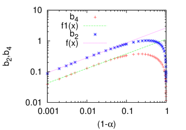
Figure 5: The decoherence parameters vanish following a power law close to $\alpha=1$. Here $f(x)=2.66(1-\alpha)^{0.487}$ and $f1(x)=1.14(1-\alpha)^{0.476}$. These data are for $n=1$.

As the centrally peaked region, assumed to behave as a delta function, is the key to the decoherence, we probe further into the region close $x=0$. Usually, decoherence effects show that the emerging centrally peaked part tends to a Gaussian form with time such that a classical behaviour (i.e. $\langle x^{2}\rangle\propto t$) is obtained at large times. (For cases where Anderson localisation takes place, the behaviour is exponential [32].) In this case, however, we find that the behaviour close to $x=0$ is definitely non-Gaussian. Rather, it shows a behaviour compatible with a power law decay for $\alpha\leq 0.9$ for $x/\sqrt{t}>1$ while for smaller values of $x/\sqrt{t}$ it is almost a constant. The curves also show negligible dependence on $\alpha$. However, the power law is valid only up to a finite value of $x/\sqrt{t}$, which depends on $\alpha$. For $\alpha$ values closer to unity, we observe that a slower stretched exponential decay fits a wider region of $x/\sqrt{t}$. These results are shown in Fig. 6. The change in behaviour from power law to stretched exponential may be an effect of the closeness to $\alpha=1$ point, where transition to a pure quantum walk occurs. The above observation shows that although the decay is power law for most values of $\alpha$, as the behaviour is limited to a finite region, and the associated exponent ($\simeq 1.7$) is not too small, the assumption that it is a delta function has worked well.

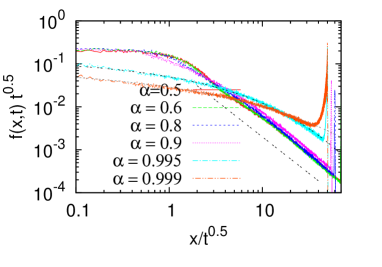
Figure 6: Behaviour of $f(x,t)$ shown for $x>0$ ($n=1$). The power law decay occurs for $x/\sqrt{t}>1$ over a finite region. The dashed line has slope equal to $-1.7$. The curves for $\alpha=0.995$ and $0.999$ are fitted to the functions $0.13\exp(-0.97x^{0.39})$ and $0.08\exp(-1.07x^{0.30})$ respectively.

3.2 Results for $n>1$

One difficulty is as $n$ increases, it is not possible to continue for very large times in the numerical simulations due to memory limitations. We have therefore considered up to $n=3$. For values of $n=2$ and $3$, $f(x,t)$ shows the existence of more peaks at intermediate points along with the two ballistic peaks and the central peak for all $0.5\leq\alpha<1$.The secondary peaks are however not as sharp as those obtained for $n=1$. Apparently, the sharpness decreases systematically with $n$. The number of secondary peaks on either sides also increases with $n$, for $n=1,2,3$ the number of prominent peaks appears to be equal to $n$ on each side.

As for $n=1$, here too we have attempted scaling collapses of $f(x,t)$ at short and long ranges (Fig. 7 shows some examples for $n=3$). While the collapse of the centrally peaked region is very good for $\alpha=0.5$, the collapse for the secondary peaks are not not so accurate in comparison; only the tips of the peaks seem to collapse. The quality of the collapses becomes poorer for $\alpha=0.995$.

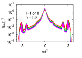
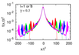
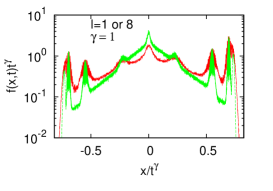
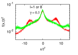
Figure 7: Scaled $f(x,t)$ for the quantum long ranged walk with step sizes 1 and 8 with probability $\alpha$ and $(1-\alpha)$. Results for $\alpha=0.5$ (top panel, with data for four $t$ values) and $0.995$ (bottom panel, with data for two $t$ values) are shown with two trial values of the scaling parameter $\gamma$.

Although the data collapses are not as good in quality as for $n=1$, $\langle x^{2}\rangle$ for $n=2$ and $3$ (shown in Fig. 8) again scale as $t^{3/2}$ asymptotically. For $\alpha=0.999$, which is very close to unity, the initial variation is like $t^{2}$ but it crosses over to a behaviour consistent with the exponent value equal to 1.5. This again shows that the minimum randomness drives the system to a novel scaling behaviour.

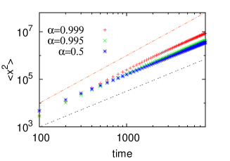
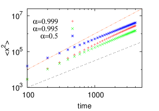
Figure 8: The second moment of $f(x,t)$ for $n=2$ (left) and $n=3$ (right) for several values of $\alpha$. The continuous lines have slopes 2 and 1.5.

.

3.3 Long ranged non-random walk

In the usual quantum walk (without randomness), the interference effects are responsible for the non-classical behaviour. To understand the present results, we argue that when the step lengths are randomly chosen, the interference effect is suppressed. For example there will be no interference when a step of unit length is followed by a step of length 2. Another reason may be that as longer steps are taken, the walker, as it moves both ways, can find itself closer to the origin with higher probability even at larger times. However, a different walk, discussed in this subsection, shows that this may be a necessary condition only and not sufficient.

In this walk, longer steps are allowed but there is no randomness. The steps here are taken in an ordered manner, for example, the walk may comprise of steps $1,2,1,2,\dots$. We note that this scheme does bring some changes in the probability density, as secondary peaks emerge (Fig. 9 shows some results for walks of different periodicities). However, the second moment still shows the conventional scaling; $\langle x^{2}\rangle\propto t^{2}$. The variation of $\langle x^{2}\rangle$ with time $t$ is shown in Fig. 10. For walks which are comparable to the $n=1,2$ and $3$ random cases, i.e., walks with periodicity 2 as steps alternate between 1 and $2^{n}$, the results are shown in the left panel. For walks of periodicity $>2$, the data plotted in the right panel of Fig. 10 show similar behaviour.

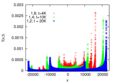
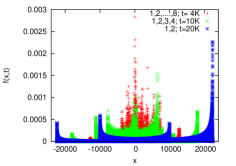
Figure 9: $f(x,t)$ for the long ranged walk without disorder shown for several cases. In the left panel, data for walks of periodicity 2 are shown while the data for periodicity $>2$ are shown in the right panel . The step lengths within one period are indicated in the key. The case for the walk 1,2,1,2…. is shown in both panels for a comparison.

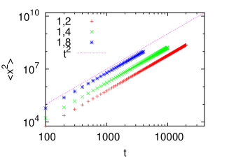
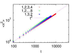
Figure 10: Second moments calculated for walks with long range steps but no randomness show usual scaling $\langle x^{2}\rangle\propto t^{2}$. Left panel - periodicity 2, right panel periodicity $>2$.

4 Summary and conclusions

A numerical study to investigate the effect of randomly chosen step lengths in a quantum walk in one dimension has been presented in this paper. The randomness introduced in the step length of the quantum walk drastically changes its nature. There is a decoherence effect but unlike in the cases studied so far, this effect does not drive it to a simple diffusive walk.

We find a new scaling behaviour $\langle x^{2}\rangle\propto t^{3/2}$ in the asymptotic limit. It is also observed that the minimum amount of disorder can drive the system to this sub-ballistic but super-diffusive scaling. The form of the distribution for $\ell$ given by eq. (3) ensures that the walker at the farthest position from the origin will not suffer any interference and hence one can expect a non-diffusive behaviour. In fact the ballistic peaks of $f(x,t)$, arising out of this dynamics show a collapse when $x$ is scaled by $t$. On the other hand, a non-Gaussian peaked region close to the origin, which collapses when $x$ is scaled by $t^{1/2}$, is also present. The result of the two effects is the novel scaling behaviour. One can compare this with the case encountered in [14], where a similar peak around the origin was noted, but in that case, it was not strong enough to affect the scaling asymptotically.

An approximate form for the moments are derived by assuming a simple form of the density profile. Two decoherence parameters are defined which vanish in a power law manner at extreme values of the disorder parameter $\alpha$ where the usual DTQW is recovered. The above observations suggest the existence of a continuous phase transition taking place at $\alpha=0$ or $1$.

Another interesting point to note is the universality of the scaling behaviour, the scaling exponent $3/2$ for $\langle x^{2}\rangle$ and $1/2$ for $\langle x\rangle$ are independent of $\alpha$, the parameter responsible for the localisation. This is in contrast to previous works where the scaling behaviour was found to depend on the disorder parameter.

Randomness is expected to localise the system, however, the simultaneous lengthening of the steps could have played a counter-role. As we note from the case without randomness, making the step lengths larger does affect the behaviour of $f(x,t)$ substantially, however, the scaling behaviour remains same. Thus one can conclude that randomness is the key ingredient responsible for the novel scaling behaviour.

While the slowing down of the walker may not be surprising in presence of the randomness, a number of other results obtained in the study are not that obvious. The form of the distribution, especially the non-Gaussian behaviour close to the origin, is not entirely predictable. The exponent $1.5$ for $\langle x^{2}\rangle$ similarly cannot be straight forwardly guessed. The universality of the exoponent value for any $\alpha\neq 0,1$ is also an interesting observation. Although the scaling exponent is not dependent on $\alpha$, its effect is present in the decoherence parameters $b_{2}$ and $b_{4}$. The results for $\langle x^{2}\rangle$ for different $\alpha$ as well as the behaviour of $b_{4}$ indicate the walker is maximally localised at $\alpha\simeq 0.8$.

A more general walk with two independent parameters where a wider spectrum of step lengths is considered also shows very similar results, a detailed study is in progress.

In the present paper, the emphasis is on the behaviour of the probability distribution $f(x,t)$ and its moments. The results already show significant departure from the conventional classical random and quantum walks. We believe these studies will inspire further characterization of the walk by addressing the issue of ‘quantumness’ of the walk [34] using other measurements.

Acknowledgement: The author thanks Charles Bennett for a very important suggestion. Financial support from SERB project, Government of India, is acknowledged.

References

- [1] R. P. Feynman and A. R. Hibbs. Quantum mechanics and path integrals. International series in pure and applied physics. McGraw-Hill, New York, (1965).
- [2] Y. Aharonov, L. Davidovich, and N. Zagury, Phys. Rev. A 48, 1687 (1993).
- [3] J. Kempe, Contemp. Phys. 44, 307 (2003).
- [4] A. Nayak and A. Vishwanath, DIAMCS Technical Report 2000-43 and Los Alamos preprint archive, quant-ph/0010117.
- [5] A. Ambainis, E. Bach, A. Nayak, A. Vishwanath, and J. Watrous, Proceedings 33rd STOC New York (͑ACM, New York, 2001).
- [6] S. E. Venegas-Andraca, Quantum Information Processing 11, 1015 (2012).
- [7] E. Farhi and S. Gutmann, Phys. Rev. A, 58, 915 (1998).
- [8] V. Kendon, Math. Struct. Comput. Sci. 17, 1169 (2007).
- [9] V. Kendon and B. Tregenna in Quantum Communication, Measureme nt and Computing (QCMC’02), Rinton Press, Princeton, NJ. Eds: J. H. Shapiro, and O. Hirota (2002); Phys. Rev. A 67, 042315 (2003).
- [10] T. A. Brun, H. A. Carteret, and A. Ambainis, Phys. Rev. Lett. 91, 130602 (2003).
- [11] T. A. Brun, H. A. Carteret, and A. Ambainis, Phys. Rev. A 67, 032304 (2003).
- [12] D. Shapira, O. Biham, A. J. Bracken and M. Hackett, Phys. Rev. A 68, 062315 (2003).
- [13] A. Romanelli, R. Siri, G. Abal, A. Auyuanet and R. Donangelo, Physica A 347, 137 (2005).
- [14] N. V. Prokof’ev and P. C. E. Stamp, Phys. Rev. A 74, R020102 (2006).
- [15] L. Ermann, J. P. Paz and M. Saraceno, Phys. Rev. A 73, 012302 (2006).
- [16] A. Romanelli, R. Siri and V. Micenmacher, Phys. Rev. E 76, 037202 (2007).
- [17] G. Abala, R. Donangeloa, F. Severoa and R. Siria, Physica A 387, 335 (2008).
- [18] A. Romanelli, Phys. Rev. A 80, 042332 (2009).
- [19] M. Annabestani, S. J. Akhtarshenas and M. R. Abolhassani, Phys. Rev. A 81, 032321 (2010).
- [20] A. Romanelli, G. Hernández, Physica A 390, 1209 (2011).
- [21] S. Fan, Z. Feng, S. Xiong and W-S. Yang, Phys. Rev. A 84, 042317 (2011).
- [22] T. Chen, Xong Zhang and Xiangdong Zhang, Sci. Rep. 7, Article number 4962 (2017).
- [23] J. Kosik, V. Buzek, and M. Hillery, Phys. Rev. A 74, 022310 (2006).
- [24] A. C. Oliveira, R. Portugal, and R. Donangelo Phys. Rev. A 74, 012312 (2006).
- [25] M. Gonulol, E. Aydiner and O. E. Mustecaplioglu, Phys. Rev. A 80, 022336 (2009).
- [26] C M Chandrashekar, and T Busch, J. Phys. A: Math. Theor. 46 105306 (2013).
- [27] T. Chen and Xangdong Zhang, Phys. Rev. A 94, 012316 (2016).
- [28] J. P. Keating, N. Linden, J. C. F. Matthews, and A. Winter, Phys. Rev. A 76, 012315 (2007).
- [29] Y. Yin, D. E. Katsanos, and S. N. Evangelou, Phys. Rev. A 77, 022302 (2008).
- [30] S Salimi and R Radgohar, J. Physics A: Math. Theor. 42, 475302 (2009).
- [31] S. Xiong and W-S Yang, J. Stat. Phys. 152, 473 (2013).
- [32] A. Schreiber, K. N. Cassemiro, V. Potocek, A. Gabris, I. Jex, and Ch. Silberhorn, Phys. Rev. Lett. 106, 180403 (2011).
- [33] M. O. Cáceres and M. Nizama, J. Phys. A: Math. Theor. 43, 455306 (2010).
- [34] R. Srikanth, S. Banerjee and C.M. Chandrashekar, Phys. Rev. A, 81, 062123 (2010).