On three genetic repressilator topologies

Abstract

Novel mathematical models of three different repressilator topologies are introduced. As designable transcription factors have been shown to bind to DNA non-cooperatively, we have chosen models containing non-cooperative elements. The extended topologies involve three additional transcription regulatory elements—which can be easily implemented by synthetic biology—forming positive feedback loops. This increases the number of variables to six, and extends the complexity of the equations in the model. To perform our analysis we had to use combinations of modern symbolic algorithms of computer algebra systems Mathematica and Singular. The study shows that all the three models have simple dynamics what can also be called regular behaviour: they have a single asymptotically stable steady state with small amplitude oscillations in the 3D case and no oscillation in one of the 6D cases and damping oscillation in the second 6D case. Using the program QeHopf we were able to exclude the presence of Hopf bifurcation in the 3D system.

1 Introduction

To understand complex biological systems such as tissues and cells, extensive knowledge of molecular interactions and mechanisms is necessary. However, an important part of understanding biological complexity is also mathematical modeling, which allows researchers to investigate connections between cellular processes and to develop hypotheses for the design of new experiments.

Jacob and Monod jacobmonod were the first to present a model of the regulation of the synthesis of a structural protein. In this model enzyme levels are regulated at the level of transcription. Specific proteins are produced which repress the transcription of the DNA to its product (mRNA – messenger ribonucleic acid), which is translated into $\beta$-galactosidase, an enzyme for degradation of galactose into simple sugars.

Shortly after Jacob and Monod, Goodwin goodwin proposed the first mathematical model of a more complex biological system, a genetic oscillator. The simplest formulation of the Goodwin model involves a single gene that represses its own transcription via a negative feedback loop and uses three variables, $x,y$ and $z$, where $x$ denotes the quantity of mRNA, $y$ stands for the quantity of the repressor protein, and $z$ is the quantity of the product, which acts as a corepressor and generates the feedback loop by negative control of mRNA production:

$$\frac{\mathrm{d}x}{\mathrm{d}t}=\frac{k_{1}}{k_{2}+z^{n}}-k_{3}x\quad\frac{\mathrm{d}y}{\mathrm{d}t}=k_{4}x-k_{5}y\quad\frac{\mathrm{d}z}{\mathrm{d}t}=k_{6}y-k_{7}z$$ (1)

All synthesis and degradation rates in the model (represented by coefficients $k_{1}$ to $k_{7}$) are linear, with the exception of the repression, which takes the form of a sigmoidal Hill curve. Here $n$ denotes the Hill exponent, which may be interpreted in biological systems as the number of ligand molecules that a receptor can bind. At the level of transcriptional regulation, this can be explained by cooperative binding of the repressor protein to DNA (formation of protein-DNA complexes). It has been demonstrated by Griffith griffith that limit cycle oscillations can only be obtained when $n>8$, which is unrealistic in terms of transcriptional regulation, where Hill exponents are rarely higher than 3 or 4.

A repressilator is a network of several genes and can be thought of as an extension of the Goodwin oscillator, which is a one-gene repressilator linked by mutual repression in a cyclic topology. Models of cycles of 2–5 genes have first been studied by Fraser and Tiwari frasertiwari , while the first experimental implementation of a 3-gene repressilator in a biological system along with a refined model was demonstrated by Elowitz and Leibler elowitzleibler . Let $X_{i}$ denote the quantity of mRNA and $Y_{i}$ the quantity of the repressor protein and let $\alpha_{0},\alpha$ and $\beta$ represent the transcription rate of a repressed promoter, the maximal transcription rate of a free promoter and the ratio of protein and mRNA decay rate, respectively. Then the model is given by the equations:

$$\frac{\mathrm{d}X_{i}}{\mathrm{d}t}= \alpha_{0}+\frac{\alpha}{1+Y_{i-1}^{n}}-X_{i}$$ (2)

$$\frac{\mathrm{d}Y_{i}}{\mathrm{d}t}= -\beta(Y_{i}-X_{i})\quad(i=1,2,3),$$

where the indices 0 and 3 are identified. (Let us note that Elowitz and Leibler write $j$ instead of $i-1$, still they speak about 6 equations. However, if $i$ and $j$ run independently, then we have $3\times 3+3=12$ equations. Our modification is also in accordance with our model below.) In the paper mentioned above Elowitz and Leibler also determine the unique positive stationary point, and the parameters when the stationary point looses its stability. They map part of the parameter space, and find oscillations numerically. In the Goodwin model, undamped oscillations can only occur when repression is accomplished by the co-repressor $Z$ and never directly by the protein $Y$ griffith , probably due to the increased time delay. In the cyclic repressilator by Elowitz and Leibler, oscillations can occur without co-repressors and for Hill exponents $n$ as low as 2, which is more applicable to biological systems. It also takes into consideration the production of mRNA with a constant rate.

A theoretical solution for the introduction of non-linearity to non-cooperative biological systems by using transcription factors, where the same proteins are able to repress one gene and activate another gene has been proposed by Müller et al. mullerhofbauerendlerflammwidderschuster and Widder et al. widdermaciasole . Tyler et al. tylershiuwalton continue the work by mullerhofbauerendlerflammwidderschuster with biologically less restrictive assumptions. However, such transcription factors are extremely rare in nature and would also be hard to design by directed evolution. Recently, Lebar et al. lebarbezeljakgolobjeralakaduncpirsstrazarvuckozupancicbencinaforstnericgaberlonzaricmajerleoblaksmolejerala have shown that non-linearity can be introduced into a biological system, by introduction of non-cooperative repressors in combination with activators, competing for binding to the same DNA sequence, thus creating a positive feedback loop. In principle, positive feedback loops could be introduced—based on the same DNA binding domain—to build functional repressilator circuits, consisting of non-cooperative repressors.

The above described oscillator circuit was experimentally constructed using three natural repressor proteins, the TetR, LacI and CI repressors. However, construction of functional biological circuits using such natural repressors requires fine-tuning due to their diverse biochemical properties. Furthermore, the low number of well-characterized natural repressor proteins does not enable construction of multiple circuits in a single cell, a fact that may support the use of stochastic models, cf. e.g. aranyitoth ; erdilente ; tothnagypapp . With the developments in the field of synthetic biology in the recent years, the use of designable repressors has become more and more frequent qilarsongilbertdoudnaweissmanarkinlim ; kianibealebrahimkhanihuhhallxieliweiss ; lohmuellerarmelsilve ; garglohmuellersilverarmel ; congzhoukuocunniffzhang ; gaberlebarmajerlesterdobnikarbencinajerala ; lebarbezeljakgolobjeralakaduncpirsstrazarvuckozupancicbencinaforstnericgaberlonzaricmajerleoblaksmolejerala ; lebarjerala ; nissimprtlifridkinperezpineralu . Such repressors can be designed to bind any DNA sequence due to their modular structure, which can be exploited to eliminate interactions with the cells’ genome. Furthermore, they can be designed in almost unlimited numbers and the biochemical properties of individual repressors are very similar, making construction and modeling of synthetic circuits easier. However, the main disadvantage of designable repressors is that they are monomeric, meaning that their binding to DNA is non-cooperative and the Hill exponent $n$ is equal to 1. Under those conditions, the above described models are not expected to produce oscillations. This poses a challenge of introducing non-linearity in complex biological systems, consisting of such repressors.

Equations describing the model of the repressilator by Elowitz and Leibler with only two variables are easy to handle. However, addition of activators to the model increases the number of variables, thus expanding the complexity of the model. Mathematical analysis of systems of equations with a large number of variables is harder, and can be investigated using deterministic approach based on ordinary differential equations (ODEs) with kinetics which can be either of the mass action type or other, and use the qualitative theory of ordinary differential equations to find bistability, oscillation etc., or calculating solutions numerically. The stochastic description (erditoth, , Chapter 5),(tothnagypapp, , Chapter 10) or erdilente usually does not allow to make symbolic calculations because of the complexity of the model. However, in this case one also may turn to the computer to do simulations sipostotherdi ; nagypapptoth .

In this work, we compare deterministic mathematical models of three different repressilator topologies based on non-cooperative repressors, which can be implemented in biological systems based on designed DNA binding domains such as zinc fingers, TALEs or dCas9/CRISPR fused to activation or repression domains. The models are simplified and consider reactions only at the protein level. The concentration of each repressor and activator over time is described in a separate equation in a system of equations. In the 3D model, we perform the singular point analysis of the 3-variable equation system for the basic repressilator topology, consisting of 3 repressors. In the 6D models we expand the complexity by addition of 3 variables, representing activators. The study of the system is non-trivial since there are no efficient methods for determining singular points of polynomial or rational systems of ODEs of high dimension and depending on parameters. We perform our analysis using the combinations of modern symbolic algorithms of computer algebra systems Mathematica mathematica and Singular deckergreuelpfisterschonemann , which has not yet been covered in the literature and represents a novel approach in analysis of biological circuits.

Extensive theoretical studies have already been done on the 3D repressilator circuit. kuznetsovafraimovich only treat the special case $\alpha_{0}=0$ of our model. In a nonlinear model such a seemingly slight difference may cause qualitative differences. They also treat saturable degradation, i.e. cases when instead of $-k_{\mathrm{deg}}x$ one has a term $\frac{-k_{\mathrm{deg}}x}{1+x}.$ They have shown the connection between the evolution of the oscillatory solution and formation of a heteroclinic cycle at infinity. dilao also deals with the $\alpha_{0}=0$ case, but he derives the usual nonlinear term starting from a mass action model, and using the Michaelis–Menten type approximation. That author is mainly interested in models with delay. guantespoyatos again assumes $\alpha_{0}=0,$ and the rational functions are such that both the denominator and the numerator are second degree polynomials. The paper contains no general mathematical statements, only numerical simulations. On the other hand, the mathematically correct paper mullerhofbauerendlerflammwidderschuster treats a large class of models including the model by Elowitz and Leibler (but not our models) and give a detailed description of the attractors. Summarizing, none of the models in the literature cover the classes of models we are interested in, and also, the present approach seems to be a novel one from the mathematical point of view and uses models based on recent experiments in synthetic biology.

Note also that tiggesmarquezlagostellingfussenegger consider a much more complicated process, no formulae can be found in the paper itself. However, its Supplement contains models, delay, stochastic effects, and no qualitative analysis at all. They estimate the parameters of the model. thieffrythomas use the heuristic ideas (kinetic logic) of Thomas without a mathematical treatment.

2 A 3D model

First we model the basic repressilator circuit based on non-cooperative repressors, similar to the Elowitz repressilator. The difference compared to the original repressilator model is that here the Hill exponent $n$ is always equal to 1, due to the non-cooperative nature of the repressors. We consider a symmetrical system, where the biochemical properties of all repressors are similar, as expected with designed transcription factors (and not to simplify mathematics). We simplify the system to only consider reactions on the protein level. The variables $x,$ $y$ and $z$ represent the concentrations of each of the repressors, while the parameters $\alpha_{0},\alpha$ and $k_{\mathrm{deg}}$ represent the rate of protein synthesis when the promoter is repressed, the maximal rate of protein synthesis from the free promoter and protein degradation rate, respectively (Figure 1).

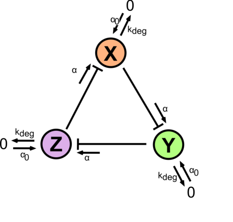
Figure 1: The 3D repressilator topology

We assume equal rates of synthesis and degradation for all three repressor proteins. Then the concentration of each repressor over time is described by the following equations:

$$\frac{dx}{dt}= \alpha_{0}+\frac{\alpha}{1+z}-k_{\mathrm{deg}}x$$ (3)

$$\frac{dy}{dt}= \alpha_{0}+\frac{\alpha}{1+x}-k_{\mathrm{deg}}y$$

$$\frac{dz}{dt}= \alpha_{0}+\frac{\alpha}{1+y}-k_{\mathrm{deg}}z,$$

To simplify the notation we denote

$$\ s=\alpha_{0},\ b=\alpha,\ g=k_{\mathrm{deg}},$$

where the parameters $s$, $b$ and $g$ are positive real numbers, and the dot denotes the derivative with respect to time.

With this notation system (3) is written as

$$\dot{x}= s+\frac{b}{1+z}-gx$$ (4)

$$\dot{y}= s+\frac{b}{1+x}-gy$$

$$\dot{z}= s+\frac{b}{1+y}-gz.$$

We are interested in the behavior of trajectories of system (4) in the region

$$D=\{(x,y,z):x>0,\ y>0,\ z>0\}.$$

System (4) has two singular points whose coordinates contain the expression $u=\sqrt{4bg+(g+s)^{2}}.$ With this we have

$$b=\frac{u^{2}-(g+s)^{2}}{4g}{\quad{\rm and}\quad u>g+s.}$$ (5)

Then the steady states of the system are

$$A=(x_{0},y_{0},z_{0})=\left(\frac{s-g-u}{2g},\frac{s-g-u}{2g},\frac{s-g-u}{2g}\right)$$

and

$$B=(x_{1},y_{1},z_{1})=\left(\frac{s+u-g}{2g},\frac{s+u-g}{2g},\frac{s+u-g}{2g}\right).$$

The eigenvalues of the Jacobian matrix of system (4) at $A$ are

$$\kappa_{1}=\frac{2gu}{g+s-u},\quad\kappa_{2,3}=-\frac{g(3g+3s-u)}{2(g+s-u)}\pm i\frac{\sqrt{3}g(g+s+u)}{2(g+s-u)}$$

and the eigenvalues at $B$ are given by

$$\lambda_{1}=-\frac{2gu}{g+s+u},\quad\lambda_{2,3}=-\frac{g(3g+3s+u)}{2(g+s+u)}\pm i\frac{\sqrt{3}g\left(g+s-u\right)}{2(g+s+u)}.$$ (6)

We can expect chemically relevant non-trivial behavior of trajectories in the domain $D$ if both singular points of the system are located in $D$. The necessary and sufficient condition for this is

$$x_{0}>0,\ x_{1}>0.$$ (7)

From $u=\sqrt{4bg+(g+s)^{2}}$, one gets both $u>g$ and $u>s$ (since $b,g$ and $s$ are positive). As a consequence, $s-g-u=(s-u)-g<0$ since $s<u.$ Thus, $A$ can be discarded. Moreover, $s+u-g=s+(u-g)>0$ since $u>g,$ so $B$ is always in the domain $D$. Thus, in this case $B$ is in $D$ and $A$ has negative coordinates. For the eigenvalues (6) of the matrix of the linear approximation of (4) at $B$ we have $\lambda_{1}<0$, $\mathrm{Re}\,\lambda_{2,3}<0$, that is, $B$ is asymptotically stable.

To conclude, in the domain $D=\{(x,y,z):x>0,\ y>0,\ z>0\}$ the system can have only one steady state (point $B$), which is a (locally) asymptotically stable attractor and the trajectories (exponentially) fast approach a neighborhood of the steady state. In a small neighborhood of it there are damping oscillations, however the amplitude of oscillations is very small. Why? Because to obtain oscillations with a large amplitude we need to have at the point $B$ in $D$ the eigenvalues with $\mathrm{Abs(Re}\,\lambda_{2,3})$ small and $\mathrm{Abs(Im}\,\lambda_{2,3})$ large. However, it can be shown easily that $\mathrm{Abs(Re}\,\lambda_{2,3})<\mathrm{Abs(Im}\,\lambda_{2,3})$ cannot occur. Thus, this is difficult to achieve in our system, while it would probably be facilitated in the system with high Hill exponent $n$. In Fig. 2 we have chosen the parameters so as to make the difference between $\mathrm{Abs(Re}\,\lambda_{2,3})$ and $\mathrm{Abs(Im}\,\lambda_{2,3})$ as small as possible. Fig. 2 shows the behaviour of the model for a single, specific set of the parameters, but the argument above is symbolic, i.e. valid for all sets of the parameters.

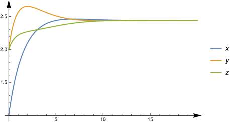
Figure 2: Damping oscillation (overshoot) in the 3D model. $s=0.3,b=4,g=0.6,$ initial concentrations: $(1,2,2).$

Our calculations above provided an alternative proof of a part of the statement by Allwright allwright who has obtained stronger results: he has shown for a class of more general class of models including our one the existence, uniqueness and global asymptotic stability of the stationary point. In order to apply Allwright’s results to our model one has to calculate a few quantities, this we will do in the Appendix 7.5.

3 The forward feedback repressilator 6D model

By a similar principle that was demonstrated to introduce a non-linear response into a non-cooperative system lebarbezeljakgolobjeralakaduncpirsstrazarvuckozupancicbencinaforstnericgaberlonzaricmajerleoblaksmolejerala , we devise a more complex repressilator topology (Figure 3). The new system consists of the same repressor topology as the 3D model, but also includes three transcriptional activators, binding to the same DNA targets as the repressors. Each of the activators drives the synthesis of itself and of the next repressor in the cycle. This topology can be implemented in biological systems using a set of three DNA binding domains (X, Y, Z), their combination with an activator (a) or a repressor (r) domain and appropriate binding sites within the three operons.

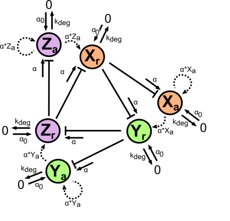
Figure 3: A repressilator topology, involving activators, driving the synthesis of the next repressor in the cycle.

The new topology therefore includes 6 variables: the concentration—denoted by the corresponding lowercase letters—of the 3 repressors ($X_{r},Y_{r}$ and $Z_{r}$) and 3 activators ($X_{a},Y_{a}$ and $Z_{a}$). The Hill exponent $n$ is always equal to 1, the parameters $\alpha_{0},\alpha$ and $k_{\mathrm{deg}}$ represent the rate of protein synthesis when the promoter is repressed, the rate of protein synthesis from the free promoter and protein degradation rate, respectively. We assume equal rates of synthesis and degradation for all repressor and activator proteins. In this case, the protein synthesis rate is considered maximal when the activator is bound to the promoter, so concentration of repressors and activators over time is given as:

$$\frac{dx_{r}}{dt}= \alpha_{0}+\alpha z_{a}/(1+z_{r}+z_{a})-k_{\mathrm{deg}}x_{r},$$ (8)

$$\frac{dz_{a}}{dt}= \alpha_{0}+\alpha z_{a}/(1+z_{r}+z_{a})-k_{\mathrm{deg}}z_{a},$$

$$\frac{dy_{r}}{dt}= \alpha_{0}+\alpha x_{a}/(1+x_{r}+x_{a})-k_{\mathrm{deg}}y_{r}$$

$$\frac{dx_{a}}{dt}= \alpha_{0}+\alpha x_{a}/(1+x_{r}+x_{a})-k_{\mathrm{deg}}x_{a},$$

$$\frac{dz_{r}}{dt}= \alpha_{0}+\alpha y_{a}/(1+y_{r}+y_{a})-k_{\mathrm{deg}}z_{r},$$

$$\frac{dy_{a}}{dt}= \alpha_{0}+\alpha y_{a}/(1+y_{r}+y_{a})-k_{\mathrm{deg}}y_{a}.$$

Introducing the notation

$$x_{1}=x_{r},\ x_{2}=z_{a},x_{3}=y_{r},\ x_{4}=x_{a},\ x_{5}=z_{r},\ x_{6}=y_{a},\ s=\alpha_{0},\ b=\alpha,\ g=k_{\mathrm{deg}}$$

where $b,g,s>0$ we rewrite system (8) in the form

$$\dot{x}_{1}= s-gx_{1}+\frac{bx_{2}}{1+x_{2}+x_{5}}=X(x_{1},x_{2},x_{5})$$ (9)

$$\dot{x}_{2}= s-gx_{2}+\frac{bx_{2}}{1+x_{2}+x_{5}}=X(x_{2},x_{2},x_{5})$$

$$\dot{x}_{3}= s-gx_{3}+\frac{bx_{4}}{1+x_{1}+x_{4}}=X(x_{3},x_{4},x_{1})$$

$$\dot{x}_{4}= s-gx_{4}+\frac{bx_{4}}{1+x_{1}+x_{4}}=X(x_{4},x_{4},x_{1})$$

$$\dot{x}_{5}= s-gx_{5}+\frac{bx_{6}}{1+x_{3}+x_{6}}=X(x_{5},x_{6},x_{3})$$

$$\dot{x}_{6}= s-gx_{6}+\frac{bx_{6}}{1+x_{3}+x_{6}}=X(x_{6},x_{6},x_{3})$$

with

$$X(u,v,w):=s-gu+\frac{bv}{1+v+w}.$$ (10)

From the first two equations of (9) we obtain that for any steady state $(x_{1},x_{2},\dots,x_{6})$ of the system it should be that $x_{1}=x_{2}$. Similarly, two other pairs of equations (9) yield that $x_{3}=x_{4},x_{5}=x_{6}.$ Thus, the simplified stationary point equations are:

$$0 = s-gx_{1}+\frac{bx_{1}}{1+x_{1}+x_{5}}=X(x_{1},x_{1},x_{5})$$ (11)

$$0 = s-gx_{3}+\frac{bx_{3}}{1+x_{1}+x_{3}}=X(x_{3},x_{3},x_{1})$$ (12)

$$0 = s-gx_{5}+\frac{bx_{5}}{1+x_{3}+x_{5}}=X(x_{5},x_{5},x_{3}).$$ (13)

We first look for steady states of system (9) using the routine Solve of Mathematica and we find 8 steady states. Two of them are

$$F=(f,f,f,f,f,f),\quad{\rm where\quad}f=\frac{\sqrt{(b-g+2s)^{2}+8gs}+b-g+2s}{4g}$$ (14)

and

$$H=(h,h,h,h,h,h),\quad{\rm where\quad}h=-\frac{\sqrt{(b-g+2s)^{2}+8gs}-b+g-2s}{4g}.$$ (15)

However, coordinates of the other steady states are given by long cumbersome expressions which are not convenient to analyse. (If one applies Simplify or even FullSimplify the result of LeafCount is more than thirteen thousand.) Thus, we choose another approach to finish.

Chemically relevant steady states should satisfy the conditions

$$X(x_{1},x_{1},x_{5})=X(x_{3},x_{3},x_{1})=X(x_{5},x_{5},x_{3})=0,\\ s>0,\ g>0,\ b>0,\ x_{1}>0,\ x_{3}>0,\ x_{5}>0.$$ (16)

System (16) is a so-called semi-algebraic system (since it contains not only algebraic equations $X(x_{1},x_{1},x_{5})=X(x_{3},x_{3},x_{1})=X(x_{5},x_{5},x_{3})=0$, but also inequalities). Nowadays powerful algorithms to solve such systems have been developed and implemented in many computer algebra systems. In particular, in Mathematica the routine Reduce can be applied to finding solutions of semi-algebraic systems. For algebraic functions Reduce constructs equivalent purely polynomial systems and then uses cylindrical algebraic decomposition (CAD) introduced by Collins in collins for real domains and Gröbner basis methods for complex domains.

To simplify computations we first clear the denominators on the right hand side of (11)–(13) obtaining the polynomials

$$f_{1} := s+bx_{1}-gx_{1}+sx_{1}-gx_{1}^{2}+sx_{5}-gx_{1}x_{5}$$

$$f_{1} := s+sx_{1}+bx_{3}-gx_{3}+sx_{3}-gx_{1}x_{3}-gx_{3}^{2}$$

$$f_{1} := s+sx_{3}+bx_{5}-gx_{5}+sx_{5}-gx_{3}x_{5}-gx_{5}^{2}0$$

Solving with Reduce of Mathematica the semi-algebraic system

$$f_{1}=f_{3}=f_{5}=0,x_{1}>0,x_{3}>0,x_{5}>0,s>0,g>0,b>0,$$ (17)

with respect to $x_{1},x_{3},x_{5},s,b,g$ we obtain the solution

$$x_{1}>0,x_{1}=x_{3}=x_{5},s>0,b>0,g=\frac{s}{x_{1}}+\frac{b}{1+x_{1}+x_{5}}.$$ (18)

The input command and the output are given in Appendix 7.3. The exact result may slightly differ depending on the version you use, but nevertheless, it always implies the essential relation that $x_{1}=x_{3}=x_{5}.$

Solving the last equation for $x_{1}$ we obtain two solutions:

$$\frac{\sqrt{(b-g+2s)^{2}+8gs}+b-g+2s}{4g}\mathrm{and}\frac{-\sqrt{(b-g+2s)^{2}+8gs}+b-g+2s}{4g}.$$

However in the second case $x_{1}$ is negative, so the only steady state whose coordinates satisfy (16) is the point $F$ defined by (14).

Computing the eigenvalues of the Jacobian matrix of system (9) at $F$ we find that they are

$$\kappa_{1,2,3} = -g,\quad\kappa_{4}=-g+\frac{b}{(1+2f)^{2}}$$

$$\kappa_{5,6} = -g+\frac{b(2+3f)}{2(1+2f)^{2}}\pm i\frac{\sqrt{3}bf}{2(1+2f)^{2}},$$

where $f$ is defined by (14). A short calculation shows that all eigenvalues of the Jacobian matrix have negative real parts yielding that $F$ is asymptotically stable. Thus, we have proven the following result.

Theorem 3.1

Point $F$ is the only positive stationary point of system (9) and it is asymptotically stable.

4 The backward feedback repressilator 6D model

Due to the absence of oscillations in the above described model we next consider a repressilator topology with activators wired to activate transcription of the previous repressor in the cycle (Figure 4). The notations of the variables and the constants are the same as in the previous 6D model. Therefore, the concentrations of repressors and activators over time are as follows:

$$\dot{x}_{1}= s-gx_{1}+bx_{4}/(1+x_{4}+x_{5})=X(x_{1},x_{4},x_{5})$$ (19)

$$\dot{x}_{2}= s-gx_{2}+bx_{4}/(1+x_{4}+x_{5})=X(x_{2},x_{4},x_{5})$$

$$\dot{x}_{3}= s-gx_{3}+bx_{6}/(1+x_{1}+x_{6})=X(x_{3},x_{6},x_{1})$$

$$\dot{x}_{4}= s-gx_{4}+bx_{6}/(1+x_{1}+x_{6})=X(x_{4},x_{6},x_{1})$$

$$\dot{x}_{5}= s-gx_{5}+bx_{2}/(1+x_{2}+x_{3})=X(x_{5},x_{2},x_{3})$$

$$\dot{x}_{6}= s-gx_{6}+bx_{2}/(1+x_{2}+x_{3})=X(x_{6},x_{2},x_{3})$$

with $X(u,v,w):=s-gu+\frac{bv}{1+v+w}$, that is, $X$ is again defined by (10), but the right-hand-sides do depend on three variables, differently form the previous case.

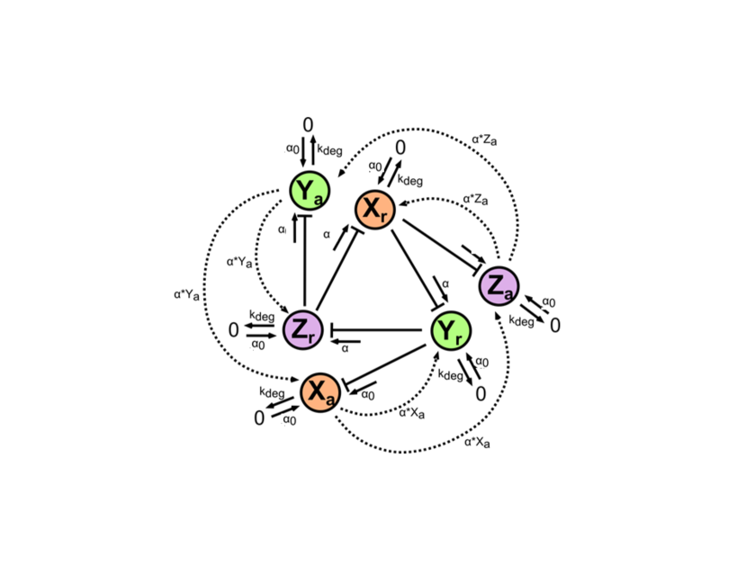
Figure 4: The backward feedback repressilator 6D model: repressilator topology including transcriptional activators, driving the synthesis of the previous repressor in the cycle.

4.1 Steady states of the model

From (19) it is easily seen that any stationary point of (19) should fulfil $x_{2}=x_{1},x_{4}=x_{3},x_{6}=x_{5}$. Then, similarly as in the case of system (9), computing with Mathematica we find that the system has singular points $F$ and $H$ defined by (14) and (15) and a few other singular points whose coordinates are given by cumbersome expressions, which are not suitable for further analysis. Therefore, again we proceed using the previous ideas.

The chemically relevant steady states of system (19) are solutions to the semi-algebraic system

$$f_{1}=f_{2}=f_{3}=0,\ s>0,\ g>0,\ b>0,\ x_{1}>0,x_{3}>0,x_{5}>0$$ (20)

where

$$f_{1}= s-gx_{1}+bx_{3}+sx_{3}-gx_{1}x_{3}+sx_{5}-gx_{1}x_{5},$$

$$f_{2}= s+sx_{1}-gx_{3}-gx_{1}x_{3}+bx_{5}+sx_{5}-gx_{3}x_{5},$$

$$f_{3}= s+bx_{1}+sx_{1}+sx_{3}-gx_{5}-gx_{1}x_{5}-gx_{3}x_{5}$$

(that is, $f_{1}=X(x_{1},x_{3},x_{5})(1+x_{3}+x_{5}),f_{2}=X(x_{3},x_{5},x_{1})(1+x_{1}+x_{5}),\ f_{3}=X(x_{5},x_{1},x_{3})(1+x_{1}+x_{3})$). But unlike the case of the previous model, we were able to solve system (20) neither with Reduce nor Solve of Mathematica. (Solve provides five roots, most of them in uselessly complicated form.) It appears that the reason is that in the previous model the steady states were determined from the system

$$X(x_{1},x_{1},x_{5})=X(x_{3},x_{3},x_{1})=X(x_{5},x_{5},x_{3})=0,$$

where each equation depended only on two variables, whereas in the present case they are to be determined from the system

$$X(x_{1},x_{3},x_{5})=X(x_{3},x_{5},x_{1})=X(x_{5},x_{1},x_{3})=0,$$

where each equation depends on three variables, so the latter system is more complicated.

To find the steady states of system (19) we use the computer algebra system Singular deckerlaplagnepfisterschonemann ; deckergreuelpfisterschonemann . We look for solutions of system

$$f_{1}(x_{1},x_{3},x_{5},s,g,b)=f_{2}(x_{1},x_{3},x_{5},s,g,b)=f_{3}(x_{1},x_{3},x_{5},s,g,b)=0.$$ (21)

The polynomials $f_{1},f_{2},f_{3}$ are polynomials of six variables with rational coefficients, that is, they are polynomials of the ring $\mathbb{Q}[s,b,g,x_{1},x_{3},x_{5}]$. In Singular the ring of such polynomials can be declared as

ring r=0,(s,b,g,x1,x3,x5),(lp)),

where r is the name of the ring, $0$ is the characteristic of the field of rational numbers $\mathbb{Q}$, and lp means that Gröbner basis calculations should be performed using the lexicographic ordering.

Let $I$ be the ideal generated by $f_{1},f_{2},f_{3}$ in $\mathbb{Q}[s,b,g,x_{1},x_{3},x_{5}]$, that is,

$$I=\langle f_{1},f_{2},f_{3}\rangle.$$ (22)

The set of solutions of system (21) is the variety $V(I)$ of $I$ (the zero set of all polynomials from $I$). (We give definitions and some facts about polynomial ideals and their varieties in Appendix 7.2.) Then, applying the routine minAssGTZ of deckergreuelpfisterschonemann , which computes minimal associate primes of polynomial ideals using the algorithm of giannitragerzacharias , we find that the variety of $I$ consists of three components,

$${\bf V}(I)={\bf V}(I_{1})\cup{\bf V}(I_{2})\cup{\bf V}(I_{3}),$$ (23)

where $I_{1},I_{2},I_{3}$ are the ideals written under [1]:, [2]: and [3]:, respectively, in Appendix 7.4.

Since $I_{1}=\langle x_{3}-x_{5},x_{1}-x_{5},2sx_{5}+s+bx_{5}-2gx_{5}^{2}-gx_{5}\rangle$ it is easily seen that the variety ${\bf V}(I_{1})$ consists of two points $F$ and $H$ defined by (14) and (15), respectively. From the equations for the third component we have $s=g=b=0$, so the system degenerates.

However, the polynomials defining the second component are complicated and difficult to analyse, so we are unable to extract useful description of the component from these polynomials.

Fortunately, there is a slightly different way to treat the problem of solving system (21). Namely, we can treat polynomials

$$f_{1}(x_{1},x_{3},x_{5},s,g,b),\ f_{2}(x_{1},x_{3},x_{5},s,g,b),\ f_{3}(x_{1},x_{3},x_{5},s,g,b)$$

as polynomials of $x_{1},x_{2},x_{3}$ depending on parameters $s,g,b$ (which is in agreement with the meaning of $s,g,b$ in differential system (19)).

To do so, we declare the ring as

ring r=(0,s,b,g),(x1,x3,x5),(lp),

where r is the name of the ring, (0,s,b,g) means that the computations should be performed in the field of characteristic 0 and s,b,g should be treated as parameters, and, as above, lp means that Gröbner basis calculations should be performed using the lexicographic ordering.

Computing with minAssGTZ the minimal associate primes of the ideal $J=\langle f_{1},f_{2},f_{3}\rangle$ (which looks as $I$ but now it is considered as the ideal of the ring $\mathbb{Q}(s,b,g)[x_{1},x_{3},x_{5}]$) we obtain that they are

$$J_{1}=\langle h_{1},h_{2},h_{3}\rangle$$

with

$$h_{1}= (2sg^{3}+bg^{3}+g^{4})x_{5}^{3}+(2s^{2}g^{2}+2sbg^{2}+5sg^{3}+2b^{2}g^{2}+2bg^{3}+2g^{4})x_{5}^{2}$$ (24)

$$+(-2s^{3}g-3s^{2}bg-s^{2}g^{2}-3sb^{2}g-2sbg^{2}+2sg^{3}-b^{3}g+g^{4})x_{5}$$

$$+(-2s^{4}-4s^{3}b-5s^{3}g-5s^{2}b^{2}-8s^{2}bg-4s^{2}g^{2}-3sb^{3}-7sb^{2}g$$

$$-5sbg^{2}-sg^{3}-b^{4}-2b^{3}g-2b^{2}g^{2}-bg^{3}),$$

$$h_{2}= (2sbg+b^{2}g+bg^{2})x_{3}+(-2sg^{2}-bg^{2}-g^{3})x_{5}^{2}$$

$$+(sbg-2sg^{2}-b^{2}g-g^{3})x_{5}$$

$$+(2s^{3}+4s^{2}b+3s^{2}g+4sb^{2}+6sbg+sg^{2}+2b^{3}+2b^{2}g+2bg^{2})$$

$$h_{3}= (2sbg+b^{2}g+bg^{2})x_{1}+(2sg^{2}+bg^{2}+g^{3})x_{5}^{2}$$

$$+(sbg+2sg^{2}+2b^{2}g+bg^{2}+g^{3})x_{5}$$

$$+(-2s^{3}-2s^{2}b-3s^{2}g-2sb^{2}-sbg-sg^{2})$$

and

$$J_{2}=\langle 2gx_{5}^{2}+(g-2s-b)x_{5}-s,x_{1}-x_{5},x_{3}-x_{5}\rangle.$$

So the variety of the ideal consists of two components

$${\bf V}(J)={\bf V}(J_{1})\cup{\bf V}(J_{2}).$$

Clearly, the variety ${\bf V}(J_{2})$ considered as a variety in $\mathbb{R}^{3}$ consists of two points $F$ and $H$ defined by (14) and (15).

Chemically relevant steady states in the component ${\bf V}(J_{1})$ are determined from the semi-algebraic system

$$b>0,\ g>0,\ s>0,x_{1}>0,x_{3}>0\ x_{5}>0,h_{1}=0,h_{2}=0,h_{3}=0.$$ (25)

Solving system (25) with Reduce we find that it has no solution (the command Reduce returns False as the output).

Using the analysis performed above we can prove the following result.

Theorem 4.1

The only steady state of system (9) with positive coordinates is the point $F$ defined by (14).

Proof

As we have shown above the only point from the variety ${\bf V}(J)$ satisfying the condition

$$b>0,\ g>0,\ s>0,x_{1}>0,x_{3}>0\ x_{5}>0$$ (26)

is the point $F$ defined by (14).

However, the complete set of steady states of system (19) is determined from the variety ${\bf V}(I)$ of the ideal $I$ defined by (22). Thus to prove the theorem it is sufficient to show that ${\bf V}(I)$ is a subset of ${\bf V}(J)$. The first components of ${\bf V}(I)$ and the second component of ${\bf V}(J)$ are the same, the third component of ${\bf V}(I)$ is the variety ${\bf V}(I_{3})$ of the ideal $I_{3}=\langle s,b,g\rangle$. Obviously, if $s=b=g=0$ then all polynomials $h_{1},h_{2},h_{3}$ vanish, that means, ${\bf V}(I_{3})$ is subset of ${\bf V}(J)$. So, we have to compare the second components of the decompositions of ${\bf V}(I)$ and ${\bf V}(J)$, that is, ${\bf V}(H)$ and ${\bf V}(G)$, where $H=\langle h_{1},h_{2},h_{3}\rangle$ with $h_{1},h_{2},h_{3}$ defined by (24) and $G=\langle g_{1},\dots,g_{11}\rangle$ where by $g_{1},\dots,g_{11}$ we denote polynomials of the second minimal associate prime given in Appendix 7.4.

First, with the command std of Singular we compute Gröbner bases of $H$ and $G$, denoting them $H_{s}$ and $G_{s}$, respectively. Then with reduce of Singular we check that $H\subset G$ (since reduce($H_{s}$,$G_{s}$) returns $0$) yielding ${\bf V}(H)\subset{\bf V}(G)$. $\square$

Remark 1

Applying the command reduce($G_{s},H_{s}$) we obtain that $H\subsetneq G$ yielding ${\bf V}(H)\subset{\bf V}(G)$, and ${\bf V}(H)$ is a strict subset of ${\bf V}(G)$ (as varieties in $\mathbb{C}^{6}$).

We also can find the precise difference of ${\bf V}(H)$ and ${\bf V}(G)$, the set ${\bf V}(H)\setminus{\bf V}(G)$. To this end, we use the fact that

$${\bf V}(H)\setminus{\bf V}(G)={\bf V}(H:G),$$

where $H:G$ is the quotient of ideals $H$ and $G$ (see e.g. coxlittleshea or romanovskishafer ). In Singular we compute the ideal $H:G$ with the command quotient(H,G) and then with minAssGTZ we compute the minimal associate primes of $H:G$ finding that the variety of $H:G$ consists of 5 components:

1) $g=s^{2}+sb+b^{2}=0$

2) $b=2s+g=0$

3) $3b-g=3s+2g=0$

4) $b=gx_{5}-s=0$,

5) $b=gx_{5}+s+g=0$

Thus, we see that the varieties ${\bf V}(H)$ and ${\bf V}(G)$ differ only for the set of parameters which are not relevant for our study: $g=0$ in case 1), $b=0$ in cases 2), 4), 5) and in case 3) $s=-2/3g$ which is impossible since $s$ and $g$ are positive.

4.2 Stability of the positive steady state

To study the stability properties of system (19) near the point $F$ we compute the characteristic polynomial $p$ of the Jacobian matrix of system (19) at $F$ and we find that it is given as

$$p(u) = \frac{(g+u)^{3}}{(1+2f)^{6}}\left(-b+g(1+2f)^{2}+u(1+2f)^{2}\right)$$

$$\left(u^{2}(1+2f)^{4}+u(1+2f)^{2}(b+2g(1+2f)^{2})\right.$$

$$+ \left.g^{2}(1+2f)^{4}+bg(1+2f)^{2}+b^{2}(1+3f+3f^{2})\right).$$

where $f$ is defined by (14). In order to prove that all the roots of the characteristic polynomial have a negative real part it is enough to show that $-b+g(1+2f)^{2}>0,$ which can be easily proven, e.g. using Reduce.

To sum up, for any $s,b,g>0$ all roots of $p$ have negative real parts. Therefore, we have proven the following statement.

Theorem 4.2

The only positive steady state $F$ of system (19) is asymptotically stable.

We can get a more precise conclusion about the eigenvalues of $F$. Computing the discriminant of the second degree factor of the above polynomial we find that it is $-3b^{2}(1+2f)^{6}<0,$ which means that the polynomial $p$ always has a pair of complex conjugate eigenvalues.

Thus, the matrix of the linear approximation of (19) at $F$ always has four negative real eigenvalues and a pair of complex conjugate eigenvalues with negative real parts. Consequently Hopf bifurcation is not possible in the system. We can expect to observe strong damping oscillations near the steady states if the absolute value of the real parts of the complex eigenvalues are much less than their imaginary parts. However our numerical experiments show that the situation appears to be just the opposite: the real parts of the complex eigenvalues are much larger than their imaginary parts. So we can observe only oscillations which quickly goes to the steady state (see Fig. 5).

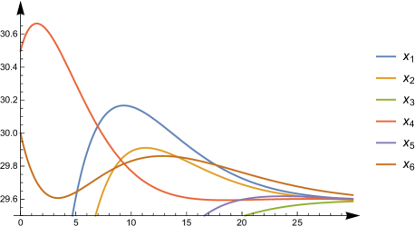
Figure 5: Damping oscillation in the 6D model. $s=1,b=10,g=0.2,$ initial concentrations: $(25,23,25,30.5,21,30)$

5 Excluding Hopf Bifurcations by Fully Algorithmic Methods

We also looked for Hopf bifurcations in the 3D and 6D models using the software package QeHopf which uses the method of the semi-algebraic characterization of Hopf bifurcation described in elkahouiweber (the package is available by request to the authors). To detect Hopf bifurcation in the models we first generate from the symbolic description of the respective ordinary differential equation a first-order formula in the language of ordered fields, where our domain is the real numbers. Specifically, for a parametrized vector field $f(u,x)$ and the autonomous ordinary differential system associated with it this semi-algebraic description can be expressed by the following first-order formula:

$$\exists x(f_{1}(u,x)=0\,\land\,f_{2}(u,x)=0\,\land\,\cdots\,\land\,f_{n}(u,x)=0$$ (27)

$$\,\land\,a_{n}>0\,\land\,\Delta_{n-1}(u,x)=0\,\land\,\Delta_{n-2}(u,x)>0\,\land\,\cdots\,\land\,\Delta_{1}(u,x)>0).$$

In this formula $a_{n}$ is $(-1)^{n}$ times the determinant of the Jacobian matrix $Df(u,x)$, and $\Delta_{i}(u,x)$ is the $i^{\rm th}$ Hurwitz determinant of the characteristic polynomial of the same matrix $Df(u,x)$. Constraints on parameters are added, and for the rational systems we are considering one is using the common numerators (adding the condition of non-vanishing denominators). QeHopf is implemented in Maple, and the input for the 3D model is as follows:

PP:=diff(x(t),t)= s-g*x(t)+b/(1+z(t)) ;
QQ:=diff(y(t),t)= s-g*y(t) +b/(1+x(t));
RR:=diff(z(t),t)= s-g*z(t)+b/(1+y(t));
fcns:={x(t), y(t) ,z(t)};
params:=[s, g, b];
paramcondlist:=[s>0, g>0, b>0];
funccondlist:=[x(t)>0, y(t)>0, z(t)>0];

DEHopfexistence({PP,QQ,RR}, fcns, params, funccondlist, paramcondlist);

For the 3D model the generated first-order formula is as follows

informula :=
 ex (vv3,  ex (vv2,  ex (vv1,  ( ( ( 0 < vv1 and  0 < vv2 ) and  0 < vv3 ) and
( ( ( ( ( ( ( s > 0 and b > 0 and g > 0 and
-g*vv1*vv3-g*vv1+s*vv3+b+s = 0 ) and
1+vv3 <> 0 ) and
-g*vv1*vv2-g*vv2+s*vv1+b+s = 0 ) and
1+vv1 <> 0 ) and
-g*vv2*vv3-g*vv3+s*vv2+b+s = 0 ) and
1+vv2 <> 0 ) and
( ( ( 0 < g^3*vv1^2*vv2^2*vv3^2+2*g^3*vv1^2*vv2^2*vv3+2*g^3*vv1^2*vv2*vv3^2
+2*g^3*vv1*vv2^2*vv3^2+g^3*vv1^2*vv2^2
+4*g^3*vv1^2*vv2*vv3+g^3*vv1^2*vv3^2+4*g^3*vv1*vv2^2*vv3
+4*g^3*vv1*vv2*vv3^2+g^3*vv2^2*vv3^2
+2*g^3*vv1^2*vv2+2*g^3*vv1^2*vv3+2*g^3*vv1*vv2^2+8*g^3*vv1*vv2*vv3
+2*g^3*vv1*vv3^2
+2*g^3*vv2^2*vv3+2*g^3*vv2*vv3^2+g^3*vv1^2+4*g^3*vv1*vv2+4*g^3*vv1*vv3
+g^3*vv2^2 +4*g^3*vv2*vv3+g^3*vv3^2+2*g^3*vv1
+2*g^3*vv2+2*g^3*vv3+b^3+g^3 and
0 < (1+vv2)^2*(1+vv3)^2*(1+vv1)^2 ) and
8*g^3*vv1^2*vv2^2*vv3^2+16*g^3*vv1^2*vv2^2*vv3+16*g^3*vv1^2*vv2*vv3^2
+16*g^3*vv1*vv2^2*vv3^2+8*g^3*vv1^2*vv2^2+32*g^3*vv1^2*vv2*vv3
+8*g^3*vv1^2*vv3^2+32*g^3*vv1*vv2^2*vv3+32*g^3*vv1*vv2*vv3^2
+8*g^3*vv2^2*vv3^2+16*g^3*vv1^2*vv2+16*g^3*vv1^2*vv3+16*g^3*vv1*vv2^2
+64*g^3*vv1*vv2*vv3+16*g^3*vv1*vv3^2+16*g^3*vv2^2*vv3+16*g^3*vv2*vv3^2
+8*g^3*vv1^2+32*g^3*vv1*vv2+32*g^3*vv1*vv3+8*g^3*vv2^2
+32*g^3*vv2*vv3+8*g^3*vv3^2
+16*g^3*vv1+16*g^3*vv2+16*g^3*vv3-b^3+8*g^3 = 0 ) and
(1+vv2)^2*(1+vv3)^2*(1+vv1)^2 <> 0 ) ) ) )  )  ) ;

The system variables became quantified variables and have been renamed to vv1, vv2, and vv3, and the existential quantification is expressed using the syntax of the package Redlog dolzmannsturm ; sturmredlog , which had been originally driven by the efficient implementation of quantifier elimination based on virtual substitution methods. Applying quantifier elimination to the formula yields in principle a quantifier-free semi-algebraic description of the parameters for which Hopf bifurcation fixed points exist.

If one suspects that there is no Hopf bifurcation fixed point or one just wants to assert that there is one, then one can apply quantifier elimination to the existential closure of our generated formula. If all variables and parameters are known to be positive, the technique of positive quantifier elimination can be used sturmweberabdelrahmanelkahoui . QeHopf uses for the quantifier elimination Redlog, which can use QEPCAD B brown for formula simplification and as fallback method. However, for the 3D model already Redlog reduces this formula to the equivalent formula false, i.e. for no parameters (obeying the positivity condition) a Hopf bifurcation fixed point exists (for positive values). The needed computation time was less than 20 ms.

For the 6D model the fully algorithmic method was not successful, as already the generation of the formula using Maple failed.

6 Discussion

Synthetic biology is one of the most rapidly developing fields of biology. Synthetic genetic circuits are of high interest due to their possible applications in biosensing, bioremediation, diagnostics, therapeutics, etc. Genetic oscillators are some of the most studied circuits due to their complexity and the possibility of many different topologies. Building synthetic genetic oscillators with controllable periods and amplitudes would be of great interest to the synthetic biology field as they could for example potentially be used for treatment of diseases related to the circadian cycle.

The experimental validation of complex systems, such as oscillators, can be technically demanding and time consuming. To this day, there has been only few experimental implementations of synthetic oscillators (elowitzleibler ; tiggesmarquezlagostellingfussenegger ). Hence, mathematical modeling of such systems is highly desirable to reduce the experimental workload. Here, we focus on mathematical modeling of 3-cycle genetic repressilators, which have been extensively studied before. However, our study is focused on models based on non-cooperative transcriptional repressors, meaning that all Hill coefficients are always equal to 1. Different studies have already demonstrated that cooperative binding is necessary to obtain oscillations in repressilator systems (elowitzleibler ; bratsunvolfsontsimringhasty ; mullerhofbauerendlerflammwidderschuster ; wangjingchen ). Our 3D model confirms that oscillations in such a system are indeed absent. However, a theoretical study by tsaichoimapomereningtangferrell has shown that the range of parameters in which the system produces oscillations can be expanded by including positive interactions, facilitated by transcriptional activators. We additionally model two repressilator topologies, involving 3 transcriptional activators, driving transcription of either the next or the previous repressor in the cycle. (Let us mention that Allwright’s results cannot be applied for our 6D models.)

What do offer the general results of formal reaction kinetics for the treatment our models? The differential equations of each of the models can be considered as induced kinetic differential equations of a reversible reaction, therefore existence of the positive stationary state follows from general results boroswrexistence ; tothnagypapp , see the details in 7.6.

To summarize our mathematical results, we have shown that for all positive values of parameters $b,g,s$ system (4) has a single positive stationary point which is a globally asymptotically stable attractor. Furthermore, (9) and (19) have a single stationary state (point $F$ defined by (14)) in the domain $x_{i}>0,\ (i=1,\dots,6)$, which is a locally asymptotically stable attractor.

Comparing the 3D and 6D models we see that the properties of solutions in the domains, where all phase variables are positive, are similar. For all the three systems in these domains there is a unique singular point which is a strong attractor. In the 3D system, a small overshoot is possible near the steady state, whereas no oscillations appear in the first 6D model near the steady state.

In both 6D models the steady state is an attractor: in both cases all eigenvalues of the steady state have negative real parts, however two eigenvalues are always complex conjugate, so it is possible to observe damping oscillations near the steady state, see Fig. 5. Thus, the 6D models demonstrate richer dynamics than the 3D models, including the possibility of damped oscillations.

We can also note that these models, as many others arising in the studying of biochemical phenomena, exhibit rather simple dynamics. It was somewhat surprising because the models are given by systems of differential equations depending on few parameters, and there are systems which look simpler, but exhibit rather complicate, even chaotic, dynamics. It can be a challenging problem to understand the reasons for such simple dynamics. One source of argument may originate in the fact the models’ stationary states are so closely related to stationary states of one linkage class reversible reactions as described in 7.6.

From the biochemical point of view, the probable reason for the absence of oscillations in the first 6D model is the strength of the activator feedback, which forms a negative feedback loop despite the positive interaction. Nevertheless, different combinations of activators and repressors could result in topologies that produce regular oscillations. Due to the stochasticity of biological systems, stochastic modeling and algorithms could be used to further analyze these topologies.

As to the computational methods: they are based on recent mathematical and algorithmic developments, and can be applied to many different similar problems frequently arising in biochemical studies. Note that theory makes it possible to turn to simpler polynomials than those at the beginning, and also that it is not the same to have a six variable polynomial and to have a three variable polynomial with three parameters.

7 Appendix

7.1 On the nonlinear term

The term $\frac{k_{1}}{k_{2}+z^{n}}$ in (1) is (from the point of calculations) similar to the one obtained when the Michaelis–Menten kinetics is approximated by Tikhonov method, or to the Holling type kinetics which is often used in population dynamics kisstoth . Therefore the methods used above may have applications in reaction kinetics and population biology, as well. The main difference between this term and the reaction rates usually used is that although this rate is always positive, it is not zero if $z$ or $x$ is zero, a general requirement quite often assumed, (volperthudjaev, , p. 613).

7.2 Solving systems of polynomial equations

We give a short summary on the topics of solving polynomial systems. The interested reader may consult coxlittleshea ; romanovskishafer for more details.

Let $k[x_{1},\ldots,x_{n}]$ denote the ring of polynomials in $n$ indeterminates with coefficients in the field $k$, which is typically the set $\mathbb{R}$ of real numbers or $\mathbb{C}$ of complex numbers.

The problem of finding solutions to a system of polynomials

$$f_{1}(x_{1},\dots,x_{n}) = 0,$$

$$\qquad\quad\ \vdots$$ (28)

$$f_{m}(x_{1},\dots,x_{n}) = 0$$

is a challenging mathematical problem. Such systems often have infinitely many solutions, and it is simply impossible to find them all numerically. Even if system (7.2) has a finite number of solutions, it is still very difficult and often impossible to find all of them numerically without applying methods of computational algebra.

In fact, no regular methods for solving system (7.2) were known until the mid-sixties of the last century when Bruno Buchberger buchberger invented the theory of Gröbner bases, which is now the cornerstone of modern computational algebra. We shall recall briefly the notion of a Gröbner basis. Let $I=\langle f_{1},f_{2},\dots,f_{s}\rangle$ denote the ideal generated by polynomials $f_{1}(x_{1},\dots,x_{n})$, $\ldots$, $f_{m}(x_{1},\dots,x_{n})$, that is, the set of all sums $\{h_{1}f_{1}+h_{2}f_{2}+\dots+h_{s}f_{s}\},$ where $f_{k},h_{k}$ are polynomials.

A Gröbner basis of a given ideal $I$ depends on a term ordering of monomials of $k[x_{1},\dots,x_{n}]$. The two most commonly used term orders are lexicographic order (lex) and degree reverse lexicographic order (degrev), defined as follows. Let ${\boldsymbol{\alpha}}=(\alpha_{1},\dots,\ \alpha_{n})$ and ${\boldsymbol{\beta}}=(\beta_{1},\dots,\beta_{n})$ be elements of $\mathbb{N}_{0}^{n}$ ($\mathbb{N}_{0}=\mathbb{N}\cup 0$). We say that ${\boldsymbol{\alpha}}>_{\rm lex}{\boldsymbol{\beta}}$ with respect to lexicographic order if and only if, reading from left to right, the first nonzero entry in the $n$-tuple ${\boldsymbol{\alpha}}-{\boldsymbol{\beta}}\in\mathbb{Z}^{n}$ is positive; we say that ${\boldsymbol{\alpha}}>_{\rm degrev}{\boldsymbol{\beta}}$   with respect to degree reverse lexicographic order if and only if $|{\boldsymbol{\alpha}}|=\sum_{j=1}^{n}\alpha_{j}>|{\boldsymbol{\beta}}|=\sum_{j=1}^{n}\beta_{j}$ or $|{\boldsymbol{\alpha}}|=|{\boldsymbol{\beta}}|\$ and, reading from right to left, the first nonzero entry in the $n$-tuple ${\boldsymbol{\alpha}}-{\boldsymbol{\beta}}\in\mathbb{Z}^{n}$ is negative. For $\gamma\in\mathbb{N}_{0}$ let ${\bf x}^{\gamma}$ denote the monomial $x_{1}^{\gamma_{1}}x_{2}^{\gamma_{2}}\cdots x_{n}^{\gamma_{n}}$. Fixing a term order on $k[x_{1},\dots,x_{n}]$, any $f\in k[x_{1},\dots,x_{n}]$ may be reordered in the standard form with respect to the order, that is,

$$f=a_{1}{\bf x}^{\alpha_{1}}+a_{2}{\bf x}^{\alpha_{2}}+\dots+a_{s}{\bf x}^{\alpha_{s}},$$ (29)

where $\alpha_{i}\neq\alpha_{j}$ for $i\neq j$ and $1\leq i,j\leq s$, and where, with respect to the specified term order, $\alpha_{1}>\alpha_{2}>\cdots>\alpha_{s}$. The leading term $LT(f)$ of $f$ is the term $LT(f)=a_{1}{\bf x}^{\alpha_{1}}$.

Let $f$ and $g$ be from $k[x_{1},\dots,x_{n}]$ with $LT(f)=a{\bf x}^{\boldsymbol{\alpha}}$ and $LT(g)=b{\bf x}^{\boldsymbol{\beta}}$. The least common multiple of ${\bf x}^{\boldsymbol{\alpha}}$ and ${\bf x}^{\boldsymbol{\beta}}$, denoted $LCM({\bf x}^{\boldsymbol{\alpha}},{\bf x}^{\boldsymbol{\beta}})$, is the monomial ${\bf x}^{\gamma}=x_{1}^{\gamma_{1}}\cdots x_{n}^{\gamma_{n}}$ such that $\gamma_{j}=\max(\alpha_{j},\beta_{j})$, $1\leq j\leq n$, and the $S$-polynomial of $f$ and $g$ is the polynomial

$$S(f,g)=\frac{{\bf x}^{\gamma}}{LT(f)}f-\frac{{\bf x}^{\gamma}}{LT(g)}g.$$

The following algorithm due to Buchberger buchberger produces a Gröbner basis for the ideal $I=\langle f_{1},\dots,f_{s}\rangle\in k[x_{1},\dots,x_{n}]$.

• $G:=\{f_{1},\dots,f_{s}\}$.

• For each pair $g_{i},g_{j}\in G$, $i\neq j$, compute the $S$-polynomial $S(g_{i},g_{j})$ and compute the remainder $r_{ij}$ of the division $S(g_{i},g_{j})$ by $G$.

• If all $r_{ij}$ are equal to zero, output $G$, else add all nonzero $r_{ij}$ to $G$ and return to Step 2.

Nowadays, all major computer algebra systems (Mathematica, Maple, REDUCE, Singular, Macaulay  and many others) have routines to compute Gröbner bases.

A Gröbner basis $G=\{g_{1},\dots,g_{m}\}$ is called reduced if for all $i$, $1\leq i\leq m$, the coefficient of the leading term is 1 and no term of $g_{i}$ is divisible by any $LT(g_{j})$ for $j\neq i$.

It is well-known (see e.g. coxlittleshea ) that system (7.2) has a solution over $\mathbb{C}$ if and only if the reduced Gröbner basis $G$ for $\langle f_{1},\dots,f_{s}\rangle$ with respect to any term order on $\mathbb{C}[x_{1},\dots,x_{n}]$ is different from $\{1\}$. The Gröbner basis theory allows to find all solutions of system (7.2) when the system has only finitely many solutions. In such case a Gröbner basis with respect to the lexicographic order is always in a “triangular” form (like the Gauss row-echelon form in the case of linear systems) which means that one has an equation in a single variable, and having solved it one can substitute the roots into an equation in two variables, solve it, etc.

For a field $k$ an affine variety is a subset of $k^{n}$ that is the solution set of a system of equations of the form (7.2), where $f_{i}$ are polynomials with coefficients in $k$. It is denoted by ${\bf V}(I)$, where $I$ is the ideal generated by $f_{1},\ldots,f_{m}$, $I:=\langle f_{1},f_{2},\dots,f_{m}\rangle$. A variety is irreducible if it is not the union of finitely many proper subsets, each of which is itself a variety. Every affine variety $V$ can be decomposed into finitely many irreducible components, that is $V$ is expressible as

$$V=V_{1}\cup\dots\cup V_{s},$$ (30)

where each $V_{j}$ is irreducible and $V_{j}\not\subset V_{k}$ if $j\neq k$, and in fact this decomposition is unique up to the ordering of the components $V_{j}$. Thus to solve (7.2) we have to find the decomposition (30) for $V={\bf V}(I)$.

A radical of the ideal $I$ is the set of polynomials $\sqrt{I}:=\{f:f^{p}\in I\text{ for some }p\in\mathbb{N}\}.$

An ideal $I\subset k[x_{1},\dots,x_{n}]$ is called a primary ideal if for any pair $f,g\in k[x_{1},\dots,x_{n}]$, $fg\in I$ only if either $f\in I$ or $g^{p}\in I$ for some $p\in\mathbb{N}$. An ideal $I$ is primary if and only if $\sqrt{I}$ is prime; $\sqrt{I}$ is called the associated prime ideal of $I$. A primary decomposition of an ideal $I\subset k[x_{1},\dots,x_{n}]$ is a representation of $I$ as a finite intersection of primary ideals $Q_{j}$, $I=\cap_{j=1}^{s}Q_{j}$ . The decomposition is called a minimal primary decomposition if the associated prime ideals $\sqrt{Q_{j}}$ are all distinct and $\cap_{i\neq j}Q_{i}\not\subset Q_{j}$ for any $j$. A minimal primary decomposition of a polynomial ideal always exists, but it is not necessarily unique.

Every ideal $I$ in $k[x_{1},\dots,x_{n}]$ has a minimal primary decomposition according to the Lasker–Noether Decomposition Theorem. All such decompositions have the same number $m$ of primary ideals and the same collection of associated prime ideals.

Minimal associate primes of a polynomial ideal $I=\langle f_{1},f_{2},\dots,f_{m}\rangle$ can be computed using the algorithm proposed by giannitragerzacharias , and the varieties of the minimal associate primes give then the irreducible decomposition of the variety $V(I)$ (so give the ”solution” to the system $f_{1}=f_{2}=\dots f_{m}=0$).

7.3 Solving Eq. (18)

Input is system (17), and the output is its solution (18).

In[20]:= Reduce[{f1 == 0 && f3 == 0 && f5 == 0 && x1 > 0 &&
    x3 > 0 && x5 > 0 && s > 0 && g > 0 && b > 0},
    {x1, x3, x5, s, b, g}] // FullSimplify

Out[20]= {x1 > 0 && x1 == x3 && x3 == x5 && s > 0 && b > 0 &&
    g == s/x1 + b/(1 + x1 + x5)}

7.4 Minimal associate primes

Minimal associate primes of ideal (22) defining the ideals $J_{1},J_{2},J_{3}$ of the decomposition (23) are:

 [1]:
   _[1]=x3-x5
   _[2]=x1-x5
   _[3]=2*s*x5+s+b*x5-2*g*x5^2-g*x5
[2]:
   _[1]=x1^3*x3+x1^3*x5+x1^3-2*x1^2*x3*x5+x1^2*x5+x1^2+x1*x3^3
   -2*x1*x3^2*x5+x1*x3^2-2*x1*x3*x5^2-6*x1*x3*x5-x1*x3+x1*x5^3
   -x1*x5+x3^3*x5+x3^3+x3^2+x3*x5^3+x3*x5^2-x3*x5+x5^3+x5^2
   _[2]=b*x3^3+b*x3^2+b*x3*x5+b*x3-b*x5^3-2*b*x5^2-b*x5
   -g*x1^2*x3^2-2*g*x1^2*x3*x5-2*g*x1^2*x3-g*x1^2*x5^2
   -2*g*x1^2*x5-g*x1^2-g*x1*x3^3+g*x1*x3^2*x5-g*x1*x3^2
   +g*x1*x3*x5^2-g*x1*x3-g*x1*x5^3-3*g*x1*x5^2-3*g*x1*x5
   -g*x1+g*x3^3*x5+2*g*x3^2*x5^2+4*g*x3^2*x5+g*x3^2+g*x3*x5^3
   +4*g*x3*x5^2+4*g*x3*x5+g*x3
   _[3]=b*x1*x5+b*x1-b*x3^2-b*x3+g*x1^2*x3+g*x1^2*x5+g*x1^2
   +g*x1*x3^2+2*g*x1*x3-g*x1*x5^2+g*x1-g*x3^2*x5-g*x3*x5^2
   -2*g*x3*x5-g*x5^2-g*x5
   _[4]=b*x1*x3+b*x3-b*x5^2-b*x5-g*x1^2*x3-g*x1^2*x5-g*x1^2
   +g*x1*x3^2-g*x1*x5^2-2*g*x1*x5-g*x1+g*x3^2*x5+g*x3^2
   +g*x3*x5^2+2*g*x3*x5+g*x3
   _[5]=b*x1^2+b*x1-b*x3*x5-b*x5+g*x1^2*x3-g*x1^2*x5+g*x1*x3^2
   +2*g*x1*x3-g*x1*x5^2-2*g*x1*x5+g*x3^2*x5+g*x3^2-g*x3*x5^2
   +g*x3-g*x5^2-g*x5
   _[6]=b^2*x3^2+b^2*x3*x5+b^2*x3+b^2*x5^2+2*b^2*x5+b^2
   +b*g*x3^2*x5+2*b*g*x3^2-b*g*x3*x5^2+b*g*x3*x5+2*b*g*x3
   +b*g*x5^2+2*b*g*x5+b*g+2*g^2*x1*x3^3+2*g^2*x1*x3^2*x5
   +3*g^2*x1*x3^2+2*g^2*x1*x3*x5^2+4*g^2*x1*x3*x5+2*g^2*x1*x3
   +2*g^2*x1*x5^3+5*g^2*x1*x5^2+4*g^2*x1*x5+g^2*x1
   +2*g^2*x3^3*x5+2*g^2*x3^3+4*g^2*x3^2*x5^2+8*g^2*x3^2*x5
   +4*g^2*x3^2+2*g^2*x3*x5^3+8*g^2*x3*x5^2+9*g^2*x3*x5
   +3*g^2*x3+2*g^2*x5^3+5*g^2*x5^2+4*g^2*x5+g^2
   _[7]=2*s*x5+s-b*x1+b*x3+b*x5-2*g*x1*x3-g*x1-g*x3+g*x5
   _[8]=2*s*x3+s+b*x1+b*x3-b*x5-2*g*x1*x5-g*x1+g*x3-g*x5
   _[9]=2*s*x1+s+b*x1-b*x3+b*x5+g*x1-2*g*x3*x5-g*x3-g*x5
   _[10]=s*b+b^2*x1+b^2*x3+b^2*x5+2*b^2+b*g*x1+b*g*x3+b*g*x5
   +2*b*g+2*g^2*x1^2*x3+2*g^2*x1^2*x5+2*g^2*x1^2+2*g^2*x1*x3^2
   +4*g^2*x1*x3*x5+6*g^2*x1*x3+2*g^2*x1*x5^2+6*g^2*x1*x5
   +4*g^2*x1+2*g^2*x3^2*x5+2*g^2*x3^2+2*g^2*x3*x5^2
   +6*g^2*x3*x5+4*g^2*x3+2*g^2*x5^2+4*g^2*x5+2*g^2
   _[11]=s^2+s*g-b^2*x1-b^2*x3-b^2*x5-b^2-b*g*x1-b*g*x3
   -b*g*x5-b*g-2*g^2*x1^2*x3-2*g^2*x1^2*x5-2*g^2*x1^2
   -2*g^2*x1*x3^2-4*g^2*x1*x3*x5-5*g^2*x1*x3-2*g^2*x1*x5^2
   -5*g^2*x1*x5-3*g^2*x1-2*g^2*x3^2*x5-2*g^2*x3^2
   -2*g^2*x3*x5^2-5*g^2*x3*x5-3*g^2*x3-2*g^2*x5^2-3*g^2*x5-g^2
[3]:
   _[1]=g
   _[2]=b
   _[3]=s

7.5 Checking the conditions of Allwright’s theorem in the 3D case

Here we strongly rely on the paper allwright : we use the definitions and notations of that paper.

His equations (5) specialize into our Eq. (4) with the following cast: $n=3$, and for $j=1,2,3:T_{j}=0,h_{j}(x)=s+\frac{b}{1+x},k_{j}(x)=-gx.$ The quantities and functions defined in this way fulfil conditions (6)–(8) in his paper. As the inverse of $k$ is $y\mapsto-y/g$ the function $\Phi$ in (9) can be calculated as

$$\frac{b^{2}g+u\left(-bg^{2}+2bgs-g^{2}s+2gs^{2}-s^{3}\right)-bg^{2}+3bgs-bs^{2}-g^{2}s+2gs^{2}-s^{3}}{gu\left(-bg+g^{2}-2gs+s^{2}\right)+g\left(-2bg+bs+g^{2}-2gs+s^{2}\right)}.$$

The derivative of $\Phi$ is negative for nonnegative arguments $u$ in accordance with the fact that the function is decreasing. Thus we have Case I with the notation of the paper. Further—lengthy—calculations show that the equation $\Phi(\Phi(u))=u$ has one positive (and one negative) real root:

$$u_{1}=\frac{-g+s+\sqrt{(g+s)^{2}+4bg}}{2g}>0,\quad u_{2}=\frac{-g+s-\sqrt{(g+s)^{2}+4bg}}{2g}<0,$$ (31)

therefore case (i) of Theorem 1 of the paper applies stating the global asymptotic stability of the unique stationary point.

7.6 Realizations with reversible reactions

Consider the equation (32) for the stationary points of the first 6D model:

$$s+bx_{1}-gx_{1}+sx_{1}-gx_{1}^{2}+sx_{5}-gx_{1}x_{5} = 0$$

$$s+sx_{1}+bx_{3}-gx_{3}+sx_{3}-gx_{1}x_{3}-gx_{3}^{2} = 0$$ (32)

$$s+sx_{3}+bx_{5}-gx_{5}+sx_{5}-gx_{3}x_{5}-gx_{5}^{2} = 0.$$

Let us note that the mass action type induced kinetic differential equation of the reaction in Fig. 6 is has exactly the right hand side equal to the left hand sides of the sbove equations if the reaction rate coefficients have appropriately been chosen. Therefore, based on the results by Orlov and Rozonoer orlovrozonoer2 ; tothnagypapp (or using the recent generalization by Boros boroswrexistence ) one can conclude that there exists a positive stationary point of the reaction, and thus, of the original (first) 6D model also has one.

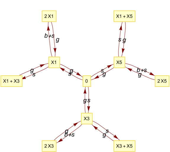
Figure 6: Feinberg–Horn–Jackson graph of a reaction leading to the stationary point of th first 6D model

The same argument can be applied in the case of the other two models.

References

- (1) Allwright, D.J.: A global stability criterion for simple control loops. J. Math. Biol. 4(4), 363–373 (1977)
- (2) Arányi, P., Tóth, J.: A full stochastic description of the Michaelis–Menten reaction for small systems. Acta Biochimica et Biophysica Academiae Scientiarum Hungaricae 12(4), 375–388 (1977)
- (3) Boros, B.: Existence of positive steady states for weakly reversible mass-action systems. arXiv preprint arXiv:1710.04732 (2017)
- (4) Bratsun, D., Volfson, D., Tsimring, L.S., Hasty, J.: Delay-induced stochastic oscillations in gene regulation. Proc. Natl. Acad. Sci. USA 102(41), 14593–14598 (2005)
- (5) Brown, C.W.: QEPCAD B: a system for computing with semi-algebraic sets via cylindrical algebraic decomposition. ACM SIGSAM Bulletin 38(1), 23–24 (2004)
- (6) Buchberger, B.: Bruno Buchberger’s PhD thesis 1965: An algorithm for finding the basis elements of the residue class ring of a zero dimensional polynomial ideal. The Journal of Symbolic Computation 41(3-4), 475–511 (2006)
- (7) Collins, G.E.: Quantifier elimination for the elementary theory of real closed fields by cylindrical algebraic decomposition. Lecture Notes in Computer Science 33, 134–183 (1975). Second GI Conference, Automata Theory and Formal Languages
- (8) Cong, L., Zhou, R., Kuo, Y., Cunniff, M., Zhang, F.: Comprehensive interrogation of natural TALE DNA-binding modules and transcriptional repressor domains. Nature Communications 3, 968 (2012)
- (9) Cox, D., Little, J., O’shea, D.: Ideals, Varieties, and Algorithms, vol. 3. Springer, New York (2007)
- (10) Decker, W., Laplagne, S., Pfister, G., Schonemann, H.A.: SINGULAR 3-1 library for computing the prime decomposition and radical of ideals, primdec.lib (2010)
- (11) Decker, W., Laplagne, S., Pfister, G., Schönemann, H.A.: SINGULAR 3-1-6—a computer algebra system for polynomial computations (2012). http://www.singular.uni-kl.de
- (12) Dilão, R.: The regulation of gene expression in eukaryotes: bistability and oscillations in repressilator models. J. Theor. Biol. 340, 199–208 (2014)
- (13) Dolzmann, A., Sturm, T.: Redlog: Computer algebra meets computer logic. ACM Sigsam Bulletin 31(2), 2–9 (1997)
- (14) El Kahoui, M., Weber, A.: Deciding Hopf bifurcations by quantifier elimination in a software-component architecture. The Journal of Symbolic Computation 30(2), 161–179 (2000)
- (15) Elowitz, M.B., Leibler, S.: A synthetic oscillatory network of transcriptional regulators. Nature 403(6767), 335–338 (2000)
- (16) Érdi, P., Lente, G.: Stochastic Chemical Kinetics. Theory and (Mostly) Systems Biological Applications. Springer Verlag (2016). Springer Series in Synergetics
- (17) Érdi, P., Tóth, J.: Mathematical Models of Chemical Reactions. Theory and Applications of Deterministic and Stochastic Models. Princeton University Press, Princeton, New Jersey (1989)
- (18) Fraser, A., Tiwari, J.: Genetical feedback-repression: II. Cyclic genetic systems. J. Theor. Biol. 47(2), 397–412 (1974)
- (19) Gaber, R., Lebar, T., Majerle, A., Šter, B., Dobnikar, A., Benčina, M., Jerala, R.: Designable DNA-binding domains enable construction of logic circuits in mammalian cells. Nature Chemical Biology 10(3), 203–208 (2014)
- (20) Garg, A., Lohmueller, J.J., Silver, P.A., Armel, T.Z.: Engineering synthetic TAL effectors with orthogonal target sites. Nucleic Acids Research 40(15), 7584–7595 (2012)
- (21) Gianni, P., Trager, B., Zacharias, G.: Gröbner bases and primary decomposition of polynomial ideals. Journal of Symbolic Computation 6(2-3), 149–167 (1988)
- (22) Goodwin, B.C.: Oscillatory behavior in enzymatic control processes. Advances in Enzyme Rregulation 3, 425–437 (1965)
- (23) Griffith, J.S.: Mathematics of cellular control processes I. Negative feedback to one gene. J. Theor. Biol. 20(2), 202–208 (1968)
- (24) Guantes, R., Poyatos, J.F.: Dynamical principles of two-component genetic oscillators. PLoS Computational Biology 2(3), e30 (2006)
- (25) Jacob, F., Monod, J.: Genetic regulatory mechanisms in the synthesis of proteins. Journal of Molecular Biology 3(3), 318–356 (1961)
- (26) Kiani, S., Beal, J., Ebrahimkhani, M.R., Huh, J., Hall, R.N., Xie, Z., Li, Y., Weiss, R.: CRISPR transcriptional repression devices and layered circuits in mammalian cells. Nature Methods 11(7), 723–726 (2014)
- (27) Kiss, K., Tóth, J.: -Dimensional ratio-dependent predator-prey systems with memory. Differential Equations and Dynamical Systems 17(1-2), 17–35 (2009)
- (28) Kuznetsov, A., Afraimovich, V.: Heteroclinic cycles in the repressilator model. Chaos, Solitons & Fractals 45(5), 660–665 (2012)
- (29) Lebar, T., Bezeljak, U., Golob, A., Jerala, M., Kadunc, L., Pirš, B., Stražar, M., Vučko, D., Zupančič, U., Benčina, M., Forstnerič, V., Gaber, R., Lonzarić, J., Majerle, A., Oblak, A., Smole, A., Jerala, R.: A bistable genetic switch based on designable DNA-binding domains. Nature Communications 5, 5007 (2014)
- (30) Lebar, T., Jerala, R.: Benchmarking of TALE-and CRISPR/dCas9-based transcriptional regulators in mammalian cells for the construction of synthetic genetic circuits. ACS Synthetic Biology 5(10), 1050–1058 (2016)
- (31) Lohmueller, J.J., Armel, T.Z., Silver, P.A.: A tunable zinc finger-based framework for boolean logic computation in mammalian cells. Nucleic Acids Research 40(11), 5180–5187 (2012)
- (32) Müller, S., Hofbauer, J., Endler, L., Flamm, C., Widder, S., Schuster, P.: A generalized model of the repressilator. J. Math. Biol. 53(6), 905–937 (2006)
- (33) Nagy, A.L., Papp, D., Tóth, J.: ReactionKinetics–A Mathematica package with applications. Chem. Eng. Sci. 83, 12–23 (2012)
- (34) Nissim, L., Perli, S.D., Fridkin, A., Perez-Pinera, P., Lu, T.K.: Multiplexed and programmable regulation of gene networks with an integrated RNA and CRISPR/Cas toolkit in human cells. Molecular Cell 54(4), 698–710 (2014)
- (35) Orlov, V.N., Rozonoer, L.I.: The macrodynamics of open systems and the variational principle of the local potential II. Applications. Journal of the Franklin Institute 318(5), 315–347 (1984)
- (36) Qi, L.S., Larson, M.H., Gilbert, L.A., Doudna, J.A., S., W.J., P., A.A., Lim, W.A.: Repurposing CRISPR as an RNA-guided platform for sequence-specific control of gene expression. Cell 152(5), 1173–1183 (2013)
- (37) Romanovski, V., Shafer, D.: The center and cyclicity problems: a computational algebra approach. Birkhäuser, Boston, Basel, Berlin (2009)
- (38) Sipos, T., Tóth, J., Érdi, P.: Stochastic simulation of complex chemical reactions by digital computer, I. The model. React. Kinet. Catal. Lett. 1(1), 113–117 (1974)
- (39) Sturm, T.: Redlog online resources for applied quantifier elimination. Acta Academiae Aboensis, Ser. B 67(2), 177–191 (2007)
- (40) Sturm, T., Weber, A., Abdel-Rahman, E.O., M., E.K.: Investigating algebraic and logical algorithms to solve Hopf bifurcation problems in algebraic biology. Mathematics in Computer Science 2(3), 493–515 (2009)
- (41) Thieffry, D., Thomas, R.: Qualitative analysis of gene networks. In: Biocomputing’98-Proceedings of The Pacific Symposium, pp. 77–88 (1997)
- (42) Tigges, M., Marquez-Lago, T.T., Stelling, J., Fussenegger, M.: A tunable synthetic mammalian oscillator. Nature 457(7227), 309–312 (2009)
- (43) Tóth, J., Nagy, A.L., Papp, D.: Reaction Kinetics: Exercises, Programs and Theorems. Springer Nature, Berlin, Heidelberg, New York (2018). In press
- (44) Tsai, T.Y., Choi, Y.S., Ma, W., Pomerening, J.R., Tang, C., Ferrell, J.E.J.: Robust, tunable biological oscillations from interlinked positive and negative feedback loops. Science 321(5885), 126–129 (2008)
- (45) Tyler, J., Shiu, A., Walton, J.: Revisiting a synthetic intracellular regulatory network that exhibits oscillations. arxiv.org (arXiv preprint arXiv:1808.00595), 1–25 (2018)
- (46) Vol’pert, A.I., Hudjaev, S.I.: Analysis in classes of discontinuous functions and the equations of mathematical physics. Martinus Nijhoff Publishers, Dordrecht, Boston, Lancaster (1985). In Russian: Nauka, Moscow, 1975
- (47) Wang, R., Jing, Z., Chen, L.: Modelling periodic oscillation in gene regulatory networks by cyclic feedback systems. Bull. Math. Biol. 67(2), 339–367 (2005)
- (48) Widder, S., Macía, J., Solé, R.: Monomeric bistability and the role of autoloops in gene regulation. PloS One 4(4), e5399 (2009)
- (49) WRI: Mathematica 11.3 (2018). http://www.wolfram.com