Mathematical analysis of transmission properties of electromagnetic meta-materials

Abstract. We study time-harmonic Maxwell’s equations in meta-materials that use either perfect conductors or high-contrast materials. Based on known effective equations for perfectly conducting inclusions, we calculate the transmission and reflection coefficients for four different geometries. For high-contrast materials and essentially two-dimensional geometries, we analyze parallel electric and parallel magnetic fields and discuss their potential to exhibit transmission through a sample of meta-material. For a numerical study, one often needs a method that is adapted to heterogeneous media; we consider here a Heterogeneous Multiscale Method for high contrast materials. The qualitative transmission properties, as predicted by the analysis, are confirmed with numerical experiments. The numerical results also underline the applicability of the multiscale method.

AMS subject classifications. 35B27, 35Q61, 65N30, 78M40

1 Introduction

Motivation. We study the transmission and reflection properties of meta-materials, i.e., of periodic microstructures of a composite material with two components. The interest in meta-materials has immensely grown in the last years as they exhibit astonishing properties such as band gaps or negative refraction; see [22, 34, 29]. The propagation of electromagnetic waves in such materials is modelled by time-harmonic Maxwell’s equations for the electric field $E$ and the magnetic field $H$:

$$\operatorname{curl}E =\phantom{-}i\omega\mu_{0}\mu H\,,$$ (1.1a)

$$\operatorname{curl}H =-i\omega\varepsilon_{0}\varepsilon E\,.$$ (1.1b)

We use the standard formulation with $\mu_{0},\varepsilon_{0}>0$ the permeability and permittivity of vacuum, $\mu$ and $\varepsilon$ the corresponding relative parameters, and $\omega>0$ the imposed frequency. While most materials are non-magnetic, i.e., $\mu=1$, the electric permittivity $\varepsilon$ covers a wide range. In this paper, we study meta-materials consisting of air (i.e., $\varepsilon=1$) and a (metal) microstructure $\Sigma_{\eta}$. The microstructure is assumed to be an $\eta$-periodic repetition of scaled copies of some geometry $\Sigma$. In the present study, we investigate in detail four different geometries: $\Sigma$ can be a metal cylinder (in two rotations), a metal plate, or the complement of an air cylinder; see Fig. 2.2 and (2.6)–(2.9) for a detailed definition. For the electric permittivity in the microstructure $\Sigma_{\eta}$, we consider two different cases: perfect conductors that are formally obtained by setting $\varepsilon=\infty$, and high-contrast materials with $\varepsilon=\varepsilon_{1}\eta^{-2}$, where $\varepsilon_{1}\in\mathbb{C}$ is some complex number with $\operatorname{Im}(\varepsilon_{1})>0$. In both cases, our study is based on the effective equations for the electric and magnetic field in the limit $\eta\to 0$.

The numerical simulation of electromagnetic wave propagation in such meta-materials is very challenging because of the rapid variations in the electric permittivity. Standard methods require the resolution of the $\eta$-scale, which often becomes infeasible even with today’s computational resources. Instead, we resort to homogenization and multiscale methods to extract macroscopic features and the behaviour of the solution. The effective equations obtained by homogenization can serve as a good motivation and starting point in this process.

Literature. Effective equations for Maxwell’s equations in meta-materials are obtained in several different settings with various backgrounds in mind: Dielectric bulk inclusions with high-contrast media [6, 7, 13] can explain the effect of artificial magnetism and lead to unusual effective permeabilities $\mu$, while long wires [5] lead to unusual effective permittivities. A combination of both structures is used to obtain a negative-index meta-material in [27]. Topological changes in the material in the limit $\eta\to 0$, such as found in split rings [10], also incite unusual effective behaviour. Perfect conductors were recently studied as well: split rings in [28] and different geometries in [36]. Finally, we briefly mention that the Helmholtz equation—as the two-dimensional reduction of Maxwell’s equations—is often studied as the first example for unusual effective properties: high-contrast inclusions in [8] or high-contrast layer materials in [11], just to name a few. An overview on this vast topic is provided in [35].

Concerning the numerical treatment, we focus on the Heterogeneous Multiscale Method (HMM) [19, 20]. For the HMM, first analytical results concerning the approximation properties for elliptic problems have been derived in [1, 21, 32] and then extended to other problems, such as time-harmonic Maxwell’s equations [25] and the Helmholtz equation and Maxwell’s equations with high-contrast [33, 37]. Another related work is the multiscale asymptotic expansion for Maxwell’s equations [12]. For further recent contributions to HMM approximations for Maxwell’s equations we refer to [16, 26]. Sparse tensor product finite elements for multiscale Maxwell-type equations are analyzed in [14] and an adaptive generalized multiscale finite element method is studied in [15].

Main results. We perform an analytical and a numerical study of transmission properties of meta-materials that contain either perfect conductors or high-contrast materials. The main results are the following:

1.) Using the effective equations of [36], we calculate the reflection and transmission coefficients for four microscopic geometries $\Sigma$. Few geometrical parameters are sufficient to fully describe the effective coefficients. We show that only certain polarizations can lead to transmission.

2.) For the two geometries that are invariant in the $\operatorname{e}_{3}$-direction, we study the limit behaviour of the electromagnetic fields for high-contrast media. When the electric field is parallel to $\operatorname{e}_{3}$, all fields vanish in the limit. Instead, when the magnetic field is parallel to $\operatorname{e}_{3}$, transmission cannot be excluded due to resonances.

3.) Extensive numerical experiments for high-contrast media confirm the analytical results. The numerical experiments underline the applicability of the Heterogeneous Multiscale Method to these challenging setting.

Some further remarks on 2.) are in order. The results are related to homogenization results of [7, 13], but we study more general geometries, since the highly conducting material can be connected. Furthermore, the results are related to [8, 11], where connected structures are investigated, but in a two-dimensional formulation. We treat here properties of the three-dimensional solutions. We emphasize that the transmission properties of a high-contrast medium cannot be captured in the framework of perfect conductors, since the latter excludes resonances on the scale of the periodicity (except if three different length-scales are considered as in [28]).

Organization of the paper. The paper is organized as follows: In Section 2, we detail the underlying problem formulations and revisit existing effective equations. In Section 3, we compute the transmission coefficients for perfect conductors and derive effective equations for high-contrast media. In Section 4, we briefly introduce the Heterogeneous Multiscale Method. Finally, in Section 5 we present several numerical experiments concerning the transmission properties of our geometries for high-contrast materials.

2 Problem formulation and effective equations

This section contains the precise formulation of the problem, including the description of the four microscopic geometries. We summarize the relevant known homogenization results and apply them to the cases of interest.

2.1 Geometry and material parameters

We study the time-harmonic Maxwell equations with linear material laws. The geometry is periodic with period $\eta>0$; solutions depend on this parameter and are therefore indexed with $\eta$. On a domain $G\subset\mathbb{R}^{3}$, the problem is to find $E^{\eta},H^{\eta}:G\to\mathbb{C}^{3}$, such that

$$\operatorname{curl}E^{\eta} =\phantom{-}i\omega\mu_{0}H^{\eta}\,,$$ (2.1a)

$$\operatorname{curl}H^{\eta} =-i\omega\varepsilon_{0}\varepsilon_{\eta}E^{\eta}\,,$$ (2.1b)

subject to appropriate boundary conditions. In the following, we will give details on the geometry $G$ and on the choice of the material parameter $\varepsilon_{\eta}$, the relative permittivity. Note that the system allows to eliminate one unknown. Indeed, if we insert $H^{\eta}$ from (2.1a) into (2.1b), we obtain

$$\operatorname{curl}\operatorname{curl}E^{\eta}=\omega^{2}\mu_{0}\varepsilon_{0}\varepsilon_{\eta}E^{\eta}\,.$$ (2.2)

Alternatively, substituting $E^{\eta}$ from (2.1b) into (2.1a), we obtain

$$\operatorname{curl}\varepsilon_{\eta}^{-1}\operatorname{curl}H^{\eta}=\omega^{2}\mu_{0}\varepsilon_{0}H^{\eta}\,.$$ (2.3)

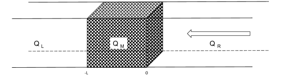
Figure 2.1: Waveguide domain $G$ with periodic scatterer $\Sigma_{\eta}$ contained in the middle part $Q_{M}$ and incident wave from the right.

Geometry. As sketched in Fig. 2.1, with positive numbers $\ell_{2},\ell_{3}>0$, the unbounded macroscopic domain is the waveguide domain

$$G\coloneqq\big{\{}x=(x_{1},x_{2},x_{3})\in\mathbb{R}^{3}\colon x_{2}\in(-\ell_{2},\ell_{2})\text{ and }x_{3}\in(-\ell_{3},\ell_{3})\big{\}}\,.$$ (2.4)

With another positive number $L>0$, the domain is divided into three parts (left, middle, right) as

$$Q_{L}\coloneqq\big{\{}x\in G\colon x_{1}\leq-L\big{\}}\,,\ Q_{M}\coloneqq\big{\{}x\in G\colon x_{1}\in(-L,0)\big{\}}\,,\ \text{ and }\ Q_{R}\coloneqq\{x\in G\colon x_{1}\geq 0\}\,.$$

The scatterer $\Sigma_{\eta}$ is contained in the middle part $Q_{M}$. For the boundary conditions, we consider an incident wave from the right that travels along the $x_{1}$-axis to the left. We restrict ourselves here to normal incidence. For the analysis, we impose periodic boundary conditions on the lateral boundaries of the domain $G$. For the numerics, we will modify the boundary conditions slightly: we truncate $G$ in $x_{1}$-direction (to obtain a bounded domain) and consider impedance boundary conditions (with the incident wave as data) on the whole boundary of $G$.

(a)

(b)

(c)

Figure 2.2: The cube shows the periodicity cell $Y$. The microstructures $\Sigma_{1}$, $\Sigma_{3}$, and $\Sigma_{4}$ are shown in dark grey. (a) The metal cylinder $\Sigma_{1}$. (b) The metal plate $\Sigma_{3}$. (c) The metal part $\Sigma_{4}$ is the complement of a cylinder.

The scatterer $\Sigma_{\eta}$ is given as an $\eta$-periodic structure. We use the periodicity cell $Y\coloneqq[-\frac{1}{2},\frac{1}{2}]^{3}$ and introduce the set $I_{\eta}$ of all vectors such that a scaled and shifted copy of $Y$ is contained in $Q_{M}$, $I_{\eta}\coloneqq\{j\in\mathbb{Z}^{3}|\eta(j+Y)\subset Q_{M}\}$. A set $\Sigma\subset Y$ specifies the meta-material, which is defined as

$$\Sigma_{\eta}\coloneqq\bigcup_{j\in I_{\eta}}\ \eta\,(j+\Sigma)\,.$$ (2.5)

For the microscopic structure $\Sigma$ we consider the following four examples. The metal cylinder (see Fig. 2.2(a)) is defined for $r\in(0,1/2)$ as

$$\Sigma_{1}\coloneqq\big{\{}y=(y_{1},y_{2},y_{3})\in Y\colon y_{1}^{2}+y_{2}^{2}<r^{2}\big{\}}\,.$$ (2.6)

The set $\Sigma_{2}$ is obtained by a rotation which aligns the cylinder with the $\operatorname{e}_{1}$-axis,

$$\Sigma_{2}\coloneqq\big{\{}y=(y_{1},y_{2},y_{3})\in Y\colon y_{2}^{2}+y_{3}^{2}<r^{2}\big{\}}\,.$$ (2.7)

To define the metal plate (see Fig. 2.2(b)), we fix $r\in(0,1/2)$ and set

$$\Sigma_{3}\coloneqq\big{\{}y=(y_{1},y_{2},y_{3})\in Y\colon y_{2}\in(-r,r)\big{\}}\,.$$ (2.8)

The fourth geometry is obtained by removing an “air cylinder” from the unit cube (see Fig. 2.2(c)); for $r\in(0,1/2)$ we set

$$\Sigma_{4}\coloneqq Y\setminus\big{\{}y=(y_{1},y_{2},y_{2})\in Y\colon y_{2}^{2}+y_{3}^{2}<r^{2}\big{\}}\,.$$ (2.9)

Material parameters. We recall that all materials are non-magnetic, the relative magnetic permeability is $\mu\equiv 1$. Outside the central region, there is no scatterer; we hence set $\varepsilon_{\eta}=1$ in $Q_{L}$ and $Q_{R}$. The middle part $Q_{M}$ contains $\Sigma_{\eta}$. We set $\varepsilon_{\eta}=1$ in $Q_{M}\setminus\Sigma_{\eta}$. It remains to specify the electric permittivity $\varepsilon_{\eta}$ in $\Sigma_{\eta}$. We consider two different settings.

(PC) In the case of perfect conductors, we set, loosely speaking, $\varepsilon_{\eta}=+\infty$ in $\Sigma_{\eta}$. More precisely, we require that $E^{\eta}$ and $H^{\eta}$ satisfy (2.1) in $G\setminus\overline{\Sigma}_{\eta}$ and $E^{\eta}=H^{\eta}=0$ in $\Sigma_{\eta}$. Boundary conditions are induced on $\partial\Sigma_{\eta}$: The magnetic field $H^{\eta}$ has a vanishing normal component and the electric field $E^{\eta}$ has vanishing tangential components on $\partial\Sigma_{\eta}$.

(HC) In the case of high-contrast media, we define the permittivity as

$$\varepsilon_{\eta}(x)\coloneqq\begin{dcases}\frac{\varepsilon_{1}}{\eta^{2}}&\text{ if }x\in\Sigma_{\eta}\,,\\ 1&\text{ if }x\in G\setminus\Sigma_{\eta}\,,\end{dcases}$$ (2.10)

where $\varepsilon_{1}\in\mathbb{C}$ with $\operatorname{Re}(\varepsilon_{1})>0$, $\operatorname{Im}(\varepsilon_{1})>0$. Physically speaking, this means that the scatterer $Q_{M}$ consists of periodically disposed metal inclusions $\Sigma_{\eta}$ embedded in vacuum. The scaling with $\eta^{2}$ means that the optical thickness of the inclusions remains constant; see [7].

In both settings and throughout this paper, we consider sequences of solutions $(E^{\eta},H^{\eta})_{\eta}$ to (2.1) which are bounded in $L^{2}(G;\mathbb{C}^{3})$,

$$\sup_{\eta>0}\int_{G}\lvert E^{\eta}\rvert^{2}+\lvert H^{\eta}\rvert^{2}<\infty\,.$$ (2.11)

Let us remark that the specific geometry of the microstructures $\Sigma_{1},\Sigma_{2}$, and $\Sigma_{4}$ is not important; the cylinders could as well be cuboids.

2.2 Effective equations

Homogenization theory allows to consider the limit $\eta\to 0$. One identifies limiting fields $\hat{E}$ and $\hat{H}$ (the latter does not coincide with the weak limit of $H^{\eta}$) and limiting equations for these fields. Using the tool of two-scale convergence, such results have been obtained for perfect conductors as well as for high-contrast materials. We briefly summarize the main findings here; analysis and numerics below are built upon these results.

Perfect conductors (PC). The homogenization analysis for this case has been performed in [36]. Since the parameters of vacuum are used outside the scatterer, the original Maxwell equations describe the limiting fields in $Q_{L}$ and $Q_{R}$. In the meta-material $Q_{M}$, however, different equations hold. There holds $E^{\eta}\operatorname*{\rightharpoonup}\hat{E}$ and $H^{\eta}\operatorname*{\rightharpoonup}\hat{\mu}\hat{H}$ in $L^{2}(G)$ and the fields $\hat{E}$ and $\hat{H}$ solve

$$\operatorname{curl}\hat{E} =\phantom{-}i\omega\mu_{0}\hat{\mu}\hat{H} \text{ in }G\,,$$ (2.12a)

$$\operatorname{curl}\hat{H} =-i\omega\varepsilon_{0}\hat{\varepsilon}\hat{E} \text{ in }G\setminus Q_{M}\,,$$ (2.12b)

$$(\operatorname{curl}\hat{H})_{k} =-i\omega\varepsilon_{0}(\hat{\varepsilon}\hat{E})_{k} \text{ in }G\,,\text{ for every }k\in\mathcal{N}_{\Sigma}\,,$$ (2.12c)

$$\hat{E}_{k} =0 \text{ in }Q_{M}\,,\text{ for every }k\in\mathcal{L}_{\Sigma}\,,$$ (2.12d)

$$\hat{H}_{k} =0 \text{ in }Q_{M}\,,\text{ for every }k\in\mathcal{N}_{Y\setminus\overline{\Sigma}}\,.$$ (2.12e)

The effective coefficients $\hat{\mu}$ and $\hat{\varepsilon}$ are determined by cell-problems. For the cell-problems, details on the index sets, and the derivation of system (2.12), we refer to [36]. The index sets $\mathcal{N}_{\Sigma}$, $\mathcal{L}_{\Sigma}$, and $\mathcal{N}_{Y\setminus\overline{\Sigma}}$ are subsets of $\{1,2,3\}$ and can be determined easily from topological properties of $\Sigma$. Loosely speaking: An index $k$ is in the set $\mathcal{L}_{\Sigma}$, if there is a curve (loop) that runs in $\Sigma$ and connects opposite faces of $Y$ in direction $\operatorname{e}_{k}$. An index $k$ is in $\mathcal{N}_{\Sigma}$, if there is no loop of that kind. We collect the index sets $\mathcal{N}_{\Sigma}$, $\mathcal{L}_{\Sigma}$, and $\mathcal{N}_{Y\setminus\overline{\Sigma}}$ for the geometries $\Sigma_{1}$ to $\Sigma_{4}$ in Table 2.1.

Table 2.1: Index sets $\mathcal{N}_{\Sigma}$, $\mathcal{L}_{\Sigma}$, and $\mathcal{N}_{Y\setminus\overline{\Sigma}}$ for microstructures $\Sigma_{1}$ to $\Sigma_{4}$ of (2.6)–(2.9).

geometry	metal cylinder $\Sigma_{1}$	metal cylinder $\Sigma_{2}$	metal plate $\Sigma_{3}$	air cylinder $\Sigma_{4}$
$\mathcal{N}_{\Sigma}$	$\{1,2\}$	$\{2,3\}$	$\{2\}$	$\emptyset$
$\mathcal{L}_{\Sigma}$	$\{3\}$	$\{1\}$	$\{1,3\}$	$\{1,2,3\}$
$\mathcal{N}_{Y\setminus\overline{\Sigma}}$	$\emptyset$	$\emptyset$	$\{2\}$	$\{2,3\}$

We will specify equations (2.12c)–(2.12e) for the four chosen geometries in Section 3.1. With the effective equations for the perfect conductors at hand, one can ask for the transmission and reflection coefficients of the meta-material. This is the goal of our analysis in Section 3.1.

high-contrast media (HC). Homogenization results for high-contrast media are essentially restricted to the case of non-connected metal parts, i.e., to geometries that are obtained by $\Sigma$ which is compactly embedded in $Y$ (it does not touch the boundary of the cube); see, e.g., [6, 10, 7]. The few exceptions are mentioned below.

For such geometries, the limit equations have again the form of Maxwell’s equations,

$$\operatorname{curl}\hat{E} =\phantom{-}i\omega\mu_{0}\hat{\mu}\hat{H} \text{ in }G\,,$$ (2.13a)

$$\operatorname{curl}\hat{H} =-i\omega\varepsilon_{0}\hat{\varepsilon}\hat{E} \text{ in }G.$$ (2.13b)

In $Q_{L}\cup Q_{R}$, the effective fields coincide with the weak limits of the original fields, and the effective relative coefficients are unit tensors. In the meta-material $Q_{M}$, however, the high-contrast in the definition of the permittivity $\varepsilon_{\eta}$ in (2.10) leads to non-trivial limit equations. The effective material parameters $\hat{\varepsilon}$ and $\hat{\mu}$ are obtained via cell problems and they can take values that are not to be expected from the choice of the material parameters in the $\eta$-problem.

As discussed in Section 2.1, time-harmonic Maxwell’s equations can equivalently be written as a single second order PDE for the $H$-field or the $E$-field. For the $H$-field we obtain

$$\operatorname{curl}\widehat{\varepsilon^{-1}}\operatorname{curl}\hat{H}=\omega^{2}\varepsilon_{0}\mu_{0}\hat{\mu}\hat{H}\qquad\text{in}\quad G\,.$$ (2.14)

Again, the effective material parameters $\widehat{\varepsilon^{-1}}$ and $\hat{\mu}$ are defined via solutions of cell problems and we refer to [13, 37] for details. We remark that the equivalence of the two formulations (2.13) and (2.14) has been shown in [37]. In particular, the effective permeability $\hat{\mu}$ agrees between both formulations and we have the relation $\widehat{\varepsilon^{-1}}=(\hat{\varepsilon})^{-1}$.

The effective equations (2.13) or (2.14) mean that, in the limit $\eta\to 0$, the meta-material $Q_{M}$ with high-contrast permittivity $\varepsilon_{\eta}$ behaves like a homogeneous material with permittivity $\hat{\varepsilon}$ and permeability $\hat{\mu}$. The occurrence of a permeability $\hat{\mu}$ in the effective equations is striking and this effect is known as artificial magnetism; see [8]. Moreover, $\hat{\mu}$ depends on the frequency $\omega$ and it can have a negative real part for certain frequencies. Negative values of the permeability are caused by (Mie) resonances in the inclusions $\Sigma$ and are studied in detail in [7, 37].

As mentioned, a crucial assumption for the homogenization analysis in [7, 13] is that $\Sigma$ is compactly contained in the unit cube. For the four geometries $\Sigma_{1}$ to $\Sigma_{4}$, this assumption is clearly not met; we therefore ask whether certain components of the effective fields $\hat{E}$ and $\hat{H}$ vanish in this case as in the case of perfect conductors. This motivates our analysis in Section 3.2 as well as the numerical experiments in Section 5.

Regarding known results on non-compactly contained inclusions we mention the thin wires in [9] and [27], and the dimensionally reduced analysis of the metal plates $\Sigma_{3}$ in [11].

3 Analysis of the microscopic geometries $\Sigma_{1}$ to $\Sigma_{4}$

In Section 3.1, we treat the case of perfect conductors and compute the transmission coefficients from the effective equations (2.12). In Section 3.2, we treat the case of high-contrast media and discuss the possibility of nontrivial transmission coefficients.

3.1 Transmission and reflection coefficients for perfect conductors

We compute the transmission and reflection coefficients for four different geometries: metal cylinders, metal plate, and air cylinder. We consider the wave guide $G=Q_{L}\cup\bar{Q}_{M}\cup Q_{R}$ of Section 2.1 and impose periodic boundary conditions on the lateral boundary of $G$. We recall that the four microscopic structures $\Sigma_{1}$ to $\Sigma_{4}$ are defined in (2.6)–(2.9). Based on the effective equations (2.12) for the perfect conductors, we compute the transmission and reflection coefficients for these geometries.

Results for perfect conductors. Before we discuss the examples in detail, we present an overview of the results. The propagation of the electromagnetic wave in vacuum is described by the time-harmonic Maxwell equations

$$\operatorname{curl}\hat{E} =\phantom{-}i\omega\mu_{0}\hat{H}\quad \text{ in }Q_{L}\cup Q_{R}\,,$$ (3.1a)

$$\operatorname{curl}\hat{H} =-i\omega\varepsilon_{0}\hat{E} \text{ in }Q_{L}\cup Q_{R}\,.$$ (3.1b)

For the electromagnetic fields, we use the time-convention $\operatorname{e}^{-i\omega t}$. From (3.1) we deduce that both fields are divergence-free in $Q_{L}\cup Q_{R}$. We shall assume that the electric field $\hat{E}\colon G\to\mathbb{C}^{3}$ in $Q_{R}$ is the superposition of a normalized incoming wave with normal incidence and a reflected wave:

$$\hat{E}(x)\coloneqq\big{(}\operatorname{e}^{-ik_{0}x_{1}}+R\operatorname{e}^{ik_{0}x_{1}}\big{)}\operatorname{e}_{k}\,,$$ (3.2)

for $x=(x_{1},x_{2},x_{3})\in Q_{R}$ and $k\in\{2,3\}$. Here, $R\in\mathbb{C}$ is the reflection coefficient and $k_{0}=\omega\sqrt{\varepsilon_{0}\mu_{0}}$. Note that the electric field $\hat{E}$ in (3.2) travels along the $x_{1}$-axis from right to left.

Due to (3.1a), the effective magnetic field $\hat{H}\colon G\to\mathbb{C}^{3}$ is given by

$$\hat{H}(x)=(-1)^{l}\frac{k_{0}}{\omega\mu_{0}}\big{(}\operatorname{e}^{-ik_{0}x_{1}}-R\operatorname{e}^{ik_{0}x_{1}}\big{)}\operatorname{e}_{l}\,,$$ (3.3)

where $l=2$ if $k=3$ and $l=3$ if $k=2$ and $x\in Q_{R}$. Equation (3.1b) is satisfied in $Q_{R}$ by our choice of $k_{0}$.

On the other hand, for the transmitted electromagnetic wave in the left domain $Q_{L}$, we make the ansatz

$$\hat{E}(x)=T\operatorname{e}^{-ik_{0}(x_{1}+L)}\operatorname{e}_{k}\quad\text{ and }\quad\hat{H}(x)=(-1)^{l}\frac{k_{0}}{\omega\mu_{0}}T\operatorname{e}^{-ik_{0}(x_{1}+L)}\operatorname{e}_{l}\,,$$ (3.4)

where $T\in\mathbb{C}$ is the transmission coefficient. We recall that $L>0$ is the width of the meta-material $Q_{M}$ and $\{x_{1}=-L\}$ is the interface between left and middle domain. Since the meta-material in $Q_{M}$ can lead to reflections, the transmission coefficient $T\in\mathbb{C}$ does not necessarily satisfy $\lvert T\rvert=1$; by energy conservation there always holds $\lvert T\rvert=1-\lvert R\rvert$.

Our results are collected in Table 3.1. The table lists transmission coefficients for the four geometries in the case that the incoming magnetic field $H$ is parallel to $\operatorname{e}_{3}$.

microstructure $\Sigma$	transmission coefficient $T$
metal cylinder $\Sigma_{1}$	$T=4p_{1}\sqrt{\alpha\gamma}\Big{[}(\alpha+\gamma)(1-p_{1}^{2})+2\sqrt{\alpha\gamma}(1+p_{1}^{2})\Big{]}^{-1}$
metal cylinder $\Sigma_{2}$	$T=4p_{2}\sqrt{\gamma}\Big{[}(1+\gamma)(1-p_{2}^{2})+2\sqrt{\gamma}(1+p_{2}^{2})\Big{]}^{-1}$
metal plate $\Sigma_{3}$	$T=4p_{0}\alpha\Big{[}(1+\alpha^{2})(1-p_{0}^{2})+2\alpha(1+p_{0}^{2})\Big{]}^{-1}$
air cylinder $\Sigma_{4}$	$T=0$

Table 3.1: Overview of the transmission coefficients $T$ when $H$ is parallel to $\operatorname{e}_{3}$. We see, in particular, that $T$ is vanishing for the structure $\Sigma_{4}$, but it is nonzero for the other micro-structures. The constant $\gamma\in\mathbb{C}$ depends on the microstructure and on solutions to cell problems, and is defined in the subsequent sections, $\alpha\coloneqq\lvert Y\setminus\Sigma\rvert$ is the volume fraction of air, $L>0$ is the width of the meta-material $Q_{M}$. We use $k_{0}=\omega\sqrt{\varepsilon_{0}\mu_{0}}$ and the numbers $p_{0}\coloneqq\operatorname{e}^{ik_{0}L}$, $p_{1}\coloneqq p_{0}\operatorname{e}^{i\sqrt{\alpha\gamma}L}$, and $p_{2}\coloneqq p_{0}\operatorname{e}^{i\sqrt{\gamma}L}$.

In the remainder of this section we compute the transmission coefficient $T$ and the reflection coefficient $R$ for the four microscopic geometries and verify, in particular, the formulas of Table 3.1. Moreover, the effective fields in the meta-material $Q_{M}$ are determined.

3.1.1 The metal cylinder $\Sigma_{1}$

The metal cylinder $\Sigma_{1}$ has a high symmetry, which allows to compute the effective permeability $\hat{\mu}$. To do so, we define the projection $\pi\colon Y\to\mathbb{R}^{2}$ onto the first two components, i.e., $\pi(y_{1},y_{2},y_{3})\coloneqq(y_{1},y_{2})$. Moreover, we set $Y^{2}\coloneqq\pi(Y)$ and $\Sigma^{2}_{1}\coloneqq\pi(\Sigma_{1})$.

Choose $l\in\{1,2\}$ and denote by $H^{l}\in L^{2}(Y;\mathbb{C}^{3})$ the distributional periodic solution of

$$\operatorname{curl}H^{l} =0 \text{ in }Y\setminus\overline{\Sigma}_{1}\,,$$ (3.5a)

$$\operatorname{div}H^{l} =0 \text{ in }Y\,,$$ (3.5b)

$$H^{l} =0 \text{ in }\Sigma_{1}\,,$$ (3.5c)

with

$$\oint H^{l}=\operatorname{e}_{l}\,.$$ (3.5d)

The normalization of the last equation is defined in [36]; loosely speaking, the left hand collects values of line integrals of $H^{l}$, where the lines are curves in $Y\setminus\Sigma$ and connect opposite faces of $Y$. Problem (3.5) is uniquely solvable by [36, Lemma 3.5]. Given the field $H^{l}=(H^{l}_{1},H^{l}_{2},H^{l}_{3})$ we define the field $h^{l}\colon Y^{2}\to\mathbb{C}^{2}$ as

$$h^{l}(y_{1},y_{2})\coloneqq\int_{0}^{1}(-H^{l}_{2},H^{l}_{1})(y_{1},y_{2},y_{3}){\,\operatorname{d}}y_{3}\,.$$ (3.6)

Lemma 3.1.

Let $H^{l}\in L^{2}(Y;\mathbb{C}^{3})$ be the solution of (3.5). Then $h^{l}\in L^{2}(Y^{2};\mathbb{C}^{2})$ of (3.6) is a distributional periodic solution to the two-dimensional problem

$$\operatorname{div}h^{l} =0 \text{ in }Y^{2}\setminus\Sigma_{1}^{2}\,,$$ (3.7a)

$$\nabla^{\bot}\cdot h^{l} =0 \text{ in }Y^{2}\,,$$ (3.7b)

$$h^{l} =0 \text{ in }\Sigma_{1}^{2}\,.$$ (3.7c)

Moreover, there exists a potential $\psi\in H_{\sharp}^{1}(Y^{2};\mathbb{C})$ such that $h^{l}=\nabla\psi-\delta_{2l}\operatorname{e}_{1}+\delta_{1l}\operatorname{e}_{2}$.

Proof.

The proof consists of a straightforward calculation. ∎

The decomposition of $h^{l}$ allows to determine the effective permeability $\hat{\mu}$, which, by [36], is given as

$$\hat{\mu}(x)\coloneqq\mu_{\operatorname{eff}}\mathds{1}_{Q_{M}}(x)+\operatorname{Id}\mathds{1}_{G\setminus\overline{Q_{M}}}(x)\,,$$ (3.8)

where

$$(\mu_{\operatorname{eff}})_{kl}\coloneqq\int_{Y}H^{l}\cdot\operatorname{e}_{k}\,.$$ (3.9)

Lemma 3.2 (Effective permeability for the metal cylinder).

For the microstructure $\Sigma=\Sigma_{1}$ the permeability $\mu_{\operatorname{eff}}$ is given by

$$\mu_{\operatorname{eff}}=\operatorname{diag}\big{(}1,1,\lvert Y\setminus\Sigma_{1}\rvert\big{)}\,.$$ (3.10)

Proof.

To shorten the notation, we write $y^{\prime}\coloneqq(y_{1},y_{2})\in Y^{2}$. Applying Fubini’s theorem and using the decomposition of $h^{1}$, we find that

$$(\mu_{\operatorname{eff}})_{11}=\int_{Y}H^{1}\cdot\operatorname{e}_{1}=\int_{Y^{2}}h^{1}_{2}(y^{\prime}){\,\operatorname{d}}y^{\prime}=\int_{Y^{2}}\partial_{2}\psi(y^{\prime}){\,\operatorname{d}}y^{\prime}+\lvert Y^{2}\rvert=1\,,$$

where, in the last equality, we exploited that $\psi$ is $Y^{2}$-periodic and that $\lvert Y^{2}\rvert=1$. A similar computation shows that ${(\mu_{\operatorname{eff}})}_{22}=1$.

To compute ${(\mu_{\operatorname{eff}})}_{12}$, we note that $h^{1}_{1}(y^{\prime})=\partial_{1}\psi(y^{\prime})$. Applying Fubini’s theorem, we find

$${(\mu_{\operatorname{eff}})}_{12}=\int_{Y}H^{1}\cdot\operatorname{e}_{2}=-\int_{Y^{2}}h^{1}_{1}(y^{\prime}){\,\operatorname{d}}y^{\prime}=-\int_{Y^{2}}\partial_{1}\psi(y^{\prime}){\,\operatorname{d}}y^{\prime}=0\,.$$

As $h^{2}_{2}(y^{\prime})=\partial_{2}\psi(y^{\prime})$, we can proceed as before and find ${(\mu_{\operatorname{eff}})}_{21}=0$.

One readily checks that $H^{3}(y)\coloneqq\mathds{1}_{Y\setminus\Sigma_{1}}(y)\operatorname{e}_{3}$ is the solution of the cell problem (3.5) with $\oint H^{3}=\operatorname{e}_{3}$. The missing entries of the effective permeability matrix $\mu_{\operatorname{eff}}$ can now be computed using the formula for $H^{3}$ and the definition of $\mu_{\operatorname{eff}}$ in (3.9). ∎

Besides $\hat{\mu}$, we also need the effective permittivity $\hat{\varepsilon}$. For $l\in\{1,2,3\}$ we denote by $E^{l}\in L^{2}(Y;\mathbb{C}^{3})$ the weak periodic solution to

$$\operatorname{curl}E^{l} =0 \text{ in }Y\,,$$ (3.11a)

$$\operatorname{div}E^{l} =0 \text{ in }Y\setminus\overline{\Sigma}_{1}\,,$$ (3.11b)

$$E^{l} =0 \text{ in }\Sigma_{1}\,,$$ (3.11c)

with

$$\int_{Y}E^{l}=\operatorname{e}_{l}\,.$$ (3.11d)

Problem (3.11) is uniquely solvable by [36, Lemma 3.1]. Consequently, the solutions to (3.11) are real vector fields. Indeed, for each index $l\in\{1,2,3\}$ the vector field $\operatorname{Im}(E^{l})\colon Y\to\mathbb{R}^{3}$ is a weak solution to (3.11) with $\int_{Y}\operatorname{Im}(E^{l})=0$ and hence $\operatorname{Im}(E^{l})=0$ in $Y$.

As in [36] we set

$$\hat{\varepsilon}(x)\coloneqq\varepsilon_{\operatorname{eff}}\mathds{1}_{Q_{M}}(x)+\operatorname{Id}\mathds{1}_{G\setminus\overline{Q_{M}}}(x)\,,$$ (3.12)

where

$$(\varepsilon_{\operatorname{eff}})_{kl}\coloneqq\int_{Y}E^{k}\cdot E^{l}\,.$$ (3.13)

Lemma 3.3 (Effective permittivity for the metal cylinder).

For the microstructure $\Sigma=\Sigma_{1}$, the permittivity $\varepsilon_{\operatorname{eff}}$ is given by

$$\varepsilon_{\operatorname{eff}}=\operatorname{diag}(\gamma,\gamma,0)\,,$$ (3.14)

where $\gamma\coloneqq({\varepsilon}_{\operatorname{eff}})_{1,1}$.

Proof.

As shown in Table 2.1, we find that $\mathcal{N}_{\Sigma_{1}}=\{1,2\}$. From [36, Lemma 3.2] we hence deduce that $(\varepsilon_{\operatorname{eff}})_{k,3}$ as well as $(\varepsilon_{\operatorname{eff}})_{3,k}$ vanish for all $k\in\{1,2,3\}$. We claim that the matrix $\varepsilon_{\operatorname{eff}}$ is symmetric. Because of $(\varepsilon_{\operatorname{eff}})_{k,3}=(\varepsilon_{\operatorname{eff}})_{3,k}=0$ we only have to prove that $(\varepsilon_{\operatorname{eff}})_{1,2}=(\varepsilon_{\operatorname{eff}})_{2,1}$. As the solutions $E^{1}$ and $E^{2}$ of the cell problem (3.11) are real vector fields, we compute that

$$(\varepsilon_{\operatorname{eff}})_{1,2}=\int_{Y}E^{1}\cdot E^{2}=\int_{Y}E^{2}\cdot E^{1}=(\varepsilon_{\operatorname{eff}})_{2,1}\,.$$

To show that $(\varepsilon_{\operatorname{eff}})_{1,2}=(\varepsilon_{\operatorname{eff}})_{2,1}=0$, we consider the map $M\colon Y\to Y$ that is defined by the diagonal matrix $\operatorname{diag}(-1,1,1)$. Note that $M(\Sigma_{1})=\Sigma_{1}$. To shorten the notation, we set $E\coloneqq E^{1}$. Consider the vector field $F\colon Y\to\mathbb{R}^{3}$,

$$F(x)\coloneqq ME(Mx)=\begin{pmatrix}-E_{1}\\ E_{2}\\ E_{3}\end{pmatrix}(-x_{1},x_{2},x_{3})\,.$$

One readily checks that $F$ is a solution to the cell problem (3.11) with $\int_{Y}F=-\operatorname{e}_{1}\,.$ Due to the unique solvability of the cell problem (3.11), we conclude that that $F=-E$. Similarly, we find that $ME^{2}\circ M=E^{2}$. Thus

$$(\varepsilon_{\operatorname{eff}})_{1,2}=\int_{Y}E^{1}\cdot E^{2}=-\int_{Y}ME^{1}(My)\cdot ME^{2}(My){\,\operatorname{d}}y=-\int_{Y}E^{1}\cdot E^{2}=-(\varepsilon_{\operatorname{eff}})_{1,2}\,.$$

Hence $(\varepsilon_{\operatorname{eff}})_{1,2}=(\varepsilon_{\operatorname{eff}})_{2,1}=0$.

We are left to prove $(\varepsilon_{\operatorname{eff}})_{2,2}=(\varepsilon_{\operatorname{eff}})_{1,1}$. To do so, we consider the rotation map $R\colon Y\to Y$ which is defined by the matrix

$$\begin{pmatrix}0&-1&0\\ 1&0&0\\ 0&0&1\end{pmatrix}\,.$$

Then $R(\Sigma_{1})=\Sigma_{1}$. Moreover, as the cell problem (3.11) is uniquely solvable, we find that $RE^{2}\circ R=-E^{1}$. Thus

$$(\varepsilon_{\operatorname{eff}})_{1,1}=\int_{Y}E^{1}\cdot E^{1}=\int_{Y}RE^{2}(Ry)\cdot RE^{2}(Ry){\,\operatorname{d}}y=\int_{Y}E^{2}\cdot E^{2}=(\varepsilon_{\operatorname{eff}})_{2,2}\,.$$

This proves the claim. ∎

By Theorem 4.1 of [36], the microstructure $\Sigma_{1}$ together with the effective permittivity from (3.14) and permeability from (3.10) implies that the effective equations are

$$\partial_{2}\hat{H}_{3}-\partial_{3}\hat{H}_{2} =-i\omega\varepsilon_{0}(\hat{\varepsilon}\hat{E})_{1} \text{ in }G\,,$$ (3.15a)

$$\partial_{3}\hat{H}_{1}-\partial_{1}\hat{H}_{3} =-i\omega\varepsilon_{0}(\hat{\varepsilon}\hat{E})_{2} \text{ in }G\,,$$ (3.15b)

$$\hat{E}_{3} =0 \text{ in }Q_{M}\,.$$ (3.15c)

The equations (3.15) do not repeat (2.12a) and (2.12b). Due to (2.12a), the effective electric field is divergence-free. As we assume that $\hat{E}$ travels along the $x_{1}$-axis, the first component $\hat{E}_{1}$ vanishes. Due to (3.15c) we expect no transmission if the effective electric field is polarized in $\operatorname{e}_{3}$-direction. For nontrivial transmission, we may therefore make the following ansatz for the effective electric field $\hat{E}\colon G\to\mathbb{C}^{3}$,

$$\hat{E}(x)\coloneqq\big{(}\operatorname{e}^{-ik_{0}x_{1}}+R\operatorname{e}^{ik_{0}x_{1}}\big{)}\operatorname{e}_{2}\quad\text{ for }x=(x_{1},x_{2},x_{3})\in Q_{R}\,.$$

Thanks to (2.12b) the magnetic field $\hat{H}$ is given by

$$\hat{H}(x)=-\frac{k_{0}}{\omega\mu_{0}}\big{(}\operatorname{e}^{-ik_{0}x_{1}}-R\operatorname{e}^{ik_{0}x_{1}}\big{)}\operatorname{e}_{3}\quad\text{ for }x=(x_{1},x_{2},x_{3})\in Q_{R}\,.$$

In the meta-material $Q_{M}$ we write

$$\hat{E}(x)=\big{(}T_{M}\operatorname{e}^{-ik_{1}x_{1}}+R_{M}\operatorname{e}^{ik_{1}x_{1}}\big{)}\operatorname{e}_{2}\text{ and }\hat{H}(x)=-\frac{k_{1}}{\omega\mu_{0}\alpha}\big{(}T_{M}\operatorname{e}^{-ik_{1}x_{1}}-R_{M}\operatorname{e}^{ik_{1}x_{1}})\operatorname{e}_{3}$$

for $x\in Q_{M}$, where we used equation (2.12a) and (3.10) to determine the magnetic field with $\alpha\coloneqq\lvert Y\setminus\Sigma_{1}\rvert$. To compute the value of $k_{0}$ we use equation (2.12b) and we find that $k_{0}=\omega\sqrt{\varepsilon_{0}\mu_{0}}$. From (3.15b) we deduce that $k_{1}=k_{0}\sqrt{\alpha\gamma}$. In $Q_{L}$ we choose (3.4) as the ansatz for $\hat{E}$ and $\hat{H}$, where $k=2$ and $l=3$.

Lemma 3.4 (Transmission and reflection coefficients).

Given the electric and magnetic fields $\hat{E}$ and $\hat{H}$ as described above. Set $\alpha\coloneqq\lvert Y\setminus\Sigma_{1}\rvert$, $k_{1}=\omega\sqrt{\varepsilon_{0}\mu_{0}\alpha\gamma}$, and $p_{1}\coloneqq\operatorname{e}^{ik_{1}L}$. The coefficients are then given by

$$R =\frac{(\alpha-\gamma)(1-p_{1}^{2})}{(\alpha+\gamma)(1-p_{1}^{2})+2\sqrt{\alpha\gamma}(1+p_{1}^{2})}\,,\quad T_{M} =\frac{2\sqrt{\alpha}(\sqrt{\alpha}+\sqrt{\gamma})}{(\alpha+\gamma)(1-p_{1}^{2})+2\sqrt{\alpha\gamma}(1+p_{1}^{2})}\,,$$

$$R_{M} =-\frac{2\sqrt{\alpha}p_{1}^{2}(\sqrt{\alpha}-\sqrt{\gamma})}{(\alpha+\gamma)(1-p_{1}^{2})+2\sqrt{\alpha\gamma}(1+p_{1}^{2})}\,,\quad T =\frac{4\sqrt{\alpha\gamma}p_{1}}{(\alpha+\gamma)(1-p_{1}^{2})+2\sqrt{\alpha\gamma}(1+p_{1}^{2})}\,.$$

Proof.

By (2.12a) the tangential trace of $\hat{E}$ has no jump across the surfaces $\{x\in G\colon x_{1}=0\}$ and $\{x\in G\colon x_{1}=-L\}$. Thus

$$T_{M}+R_{M}=1+R\quad\text{ and }\quad T=p_{1}T_{M}+\frac{1}{p}_{1}R_{M}\,.$$ (3.16)

The effective field $\hat{H}$ is parallel to $\operatorname{e}_{3}$ and hence, by (3.15b), the third component $\hat{H}_{3}$ does not jump across the surfaces $\{x\in G\colon x_{1}=0\}$ and $\{x\in G\colon x_{1}=-L\}$. We may therefore conclude that

$$\sqrt{\frac{\gamma}{\alpha}}\big{(}T_{M}-R_{M}\big{)}=1-R\quad\text{ and }\quad T=\sqrt{\frac{\gamma}{\alpha}}\bigg{(}p_{1}T_{M}-\frac{1}{p}_{1}R_{M}\bigg{)}\,.$$ (3.17)

Here we used that $k_{0}=\omega\sqrt{\mu_{0}\varepsilon_{0}}$ and $k_{1}=k_{0}\sqrt{\alpha\gamma}$. Solving the equations on the left-hand side in (3.16) and (3.17) for $R$ and the other two equations for $T$, we find that

$$T_{M}+R_{M}-1 =R=1-\sqrt{\frac{\gamma}{\alpha}}(T_{M}-R_{M})$$ (3.18)

and

$$p_{1}T_{M}+\frac{1}{p_{1}}R_{M} =T=\sqrt{\frac{\gamma}{\alpha}}\bigg{(}p_{1}T_{M}-\frac{1}{p_{1}}R_{M}\bigg{)}\,.$$ (3.19)

Setting $d_{+}\coloneqq 1+\sqrt{\gamma/\alpha}$ and $d_{-}\coloneqq 1-\sqrt{\gamma/\alpha}$, equations (3.18) and (3.1.1) can be written as

$$d_{+}T_{M}=2-d_{-}R_{M}\quad\text{ and }\quad p_{1}d_{-}T_{M}=-\frac{1}{p_{1}}d_{+}R_{M}\,.$$ (3.20)

Solving each of the two equations in (3.20) for $R_{M}$ and then equating the two expressions for $R_{M}$, we obtain

$$T_{M} =\frac{2d_{+}}{d_{+}^{2}-d_{-}^{2}p_{1}^{2}}=\frac{2(1+\sqrt{\gamma/\alpha})}{(1+\sqrt{\gamma/\alpha})^{2}-(1-\sqrt{\gamma/\alpha})^{2}p_{1}^{2}}=\frac{2\sqrt{\alpha}(\sqrt{\alpha}+\sqrt{\gamma})}{(\sqrt{\alpha}+\sqrt{\gamma})^{2}-(\sqrt{\alpha}-\sqrt{\gamma})^{2}p_{1}^{2}}\,.$$

Note that $(\sqrt{\alpha}+\sqrt{\gamma})^{2}-(\sqrt{\alpha}-\sqrt{\gamma})^{2}p_{1}^{2}=(\alpha+\gamma)(1-p_{1}^{2})+2\sqrt{\alpha\gamma}(1+p_{1}^{2})$, which yields the formula for $T_{M}$. From the second equation in (3.20), we deduce that

$$R_{M}=-p_{1}^{2}\frac{d_{-}}{d_{+}}T_{M}=-p_{1}^{2}\frac{\sqrt{\alpha}-\sqrt{\gamma}}{\sqrt{\alpha}+\sqrt{\gamma}}T_{M}=-\frac{2\sqrt{\alpha}p_{1}^{2}(\sqrt{\alpha}-\sqrt{\gamma})}{(\alpha+\gamma)(1-p_{1}^{2})+2\sqrt{\alpha\gamma}(1+p_{1}^{2})}\,.$$

By (3.18), we have that

$$R =T_{M}+R_{M}-1=\frac{2\sqrt{\alpha}(\sqrt{\alpha}+\sqrt{\gamma})-2\sqrt{\alpha}p_{1}^{2}(\sqrt{\alpha}-\sqrt{\gamma})}{(\alpha+\gamma)(1-p_{1}^{2})+2\sqrt{\alpha\gamma}(1+p_{1}^{2})}-1$$

$$=\frac{(\alpha-\gamma)(1-p_{1}^{2})}{(\alpha+\gamma)(1-p_{1}^{2})+2\sqrt{\alpha\gamma}(1+p_{1}^{2})}\,.$$

To compute the coefficient $T$ we use equation (3.16) and find that

$$T =\frac{2\sqrt{\alpha}(\sqrt{\alpha}+\sqrt{\gamma})p_{1}-2\sqrt{\alpha}(\sqrt{\alpha}-\sqrt{\gamma})p_{1}}{(\alpha+\gamma)(1-p_{1}^{2})+2\sqrt{\alpha\gamma}(1+p_{1}^{2})}=\frac{4\sqrt{\alpha}\sqrt{\gamma}p_{1}}{(\alpha+\gamma)(1-p_{1}^{2})+2\sqrt{\alpha\gamma}(1+p_{1}^{2})}\,.$$

This proves the claim. ∎

3.1.2 The metal cylinder $\Sigma_{2}$

Similar to the previous section, we shall determine the transmission and reflection coefficients for a metal cylinder, considering the microstructure $\Sigma_{2}$. We define the effective permeability and the effective permittivity $\hat{\mu},\hat{\varepsilon}\colon G\to\mathbb{C}^{3}$ as in (3.8) and (3.12). Following the reasoning of Section 3.1.1, we find that the $\mu_{\operatorname{eff}}$ and $\varepsilon_{\operatorname{eff}}$ are given by

$$\mu_{\operatorname{eff}}=\operatorname{diag}\big{(}\lvert Y\setminus\Sigma_{2}\rvert,1,1\big{)}\quad\text{ and }\quad\varepsilon_{\operatorname{eff}}=\operatorname{diag}(0,\gamma,\gamma)\,,$$

where $\gamma\in\mathbb{C}$ is defined as $\gamma\coloneqq\int_{Y}E^{2}\cdot E^{2}$. The effective equations for the microstructure $\Sigma_{2}$ are

$$\partial_{3}\hat{H}_{1}-\partial_{1}\hat{H}_{3} =-i\omega\varepsilon_{0}(\hat{\varepsilon}\hat{E})_{2} \text{ in }G\,,$$ (3.21a)

$$\partial_{1}\hat{H}_{2}-\partial_{2}\hat{H}_{1} =-i\omega\varepsilon_{0}(\hat{\varepsilon}\hat{E})_{3} \text{ in }G\,,$$ (3.21b)

$$\hat{E}_{1} =0 \text{ in }Q_{M}\,.$$ (3.21c)

We may take a similar ansatz for the effective fields as in Section 3.1.1 and obtain the following transmission and reflection coefficients. Note that $k_{1}$ in Section 3.1.1 has to be replaced by $k_{2}\coloneqq k_{0}\sqrt{\gamma}$.

Lemma 3.5 (Transmission and reflection coefficients).

Within the setting of Section 3.1.1, we set $k_{2}=\omega\sqrt{\varepsilon_{0}\mu_{0}\gamma}$ and $p_{2}\coloneqq e^{ik_{2}L}$. The reflection and transmission coefficients for $\Sigma_{2}$ are given by

$$R =\frac{(1-\gamma)(1-p_{2}^{2})}{(1+\gamma)(1-p_{2}^{2})+2\sqrt{\gamma}(1+p_{2}^{2})}\,, T_{M} =\frac{2(1+\sqrt{\gamma})}{(1+\gamma)(1-p_{2}^{2})+2\sqrt{\gamma}(1+p_{2}^{2})}\,,$$

$$R_{M} =-\frac{2p_{2}^{2}(1-\sqrt{\gamma})}{(1+\gamma)(1-p_{2}^{2})+2\sqrt{\gamma}(1+p_{2}^{2})}\,, T =\frac{4p_{2}\sqrt{\gamma}}{(1+\gamma)(1-p_{2}^{2})+2\sqrt{\gamma}(1+p_{2}^{2})}\,.$$

Note that in the above transmission and reflection coefficients the volume fraction of air $\alpha=\lvert Y\setminus\Sigma_{2}\rvert$ does not appear. This is different for the metal cylinder $\Sigma_{1}$; see Lemma 3.4.

Proof.

Thanks to (2.12a) we know that the tangential components of $\hat{E}$ do not jump across the surfaces $\{x\in G\colon x_{1}=0\}$ and $\{x\in G\colon x_{1}=-L\}$. Hence

$$1+R=T_{M}+R_{M}\quad\text{ and }T=p_{2}T_{M}+\frac{1}{p_{2}}R_{M}\,.$$ (3.22)

The effective field $\hat{H}$ is parallel to $\operatorname{e}_{3}$ and hence, due to (3.21a), the third component $\hat{H}_{3}$ does neither jump across $\{x\in G\colon x_{1}=0\}$ nor across $\{x\in G\colon x_{1}=-L\}$. We may therefore conclude that

$$1-R=\sqrt{\gamma}(T_{M}-R_{M})\quad\text{ and }\quad T=\sqrt{\gamma}\bigg{(}p_{2}T_{M}-\frac{1}{p_{2}}R_{M}\bigg{)}\,.$$ (3.23)

Here we used that $k_{2}=k_{0}\sqrt{\gamma}=\omega\sqrt{\varepsilon_{0}\mu_{0}\gamma}$.

Solving the equations on the left-hand side in (3.22) and (3.23) for $R$ and the other two for $T$, we find that

$$T_{M}+R_{M}-1=R=1-\sqrt{\gamma}(T_{M}-R_{M})\>\text{ and }\>p_{2}T_{M}+\frac{1}{p_{2}}R_{M}=T=\sqrt{\gamma}\bigg{(}p_{2}T_{M}-\frac{1}{p_{2}}R_{M}\bigg{)}\,.$$

Setting $c_{+}\coloneqq 1+\sqrt{\gamma}$ and $c_{-}\coloneqq 1-\sqrt{\gamma}$, these two equations can be re-written as

$$c_{+}T_{M}=2-c_{-}R_{M}\quad\text{ and }\quad c_{-}p_{2}T_{M}=-\frac{1}{p_{2}}c_{+}R_{M}\,.$$ (3.24)

We can solve for $T_{M}$ and obtain

$$T_{M}=\frac{2c_{+}}{c_{+}^{2}-c_{-}^{2}p_{2}^{2}}=\frac{2(1+\sqrt{\gamma})}{(1+\sqrt{\gamma})^{2}-(1-\sqrt{\gamma})^{2}p_{2}^{2}}\,.$$

Note that $(1+\sqrt{\gamma})^{2}-(1-\sqrt{\gamma})^{2}p_{2}^{2}=(1+\gamma)(1-p_{2}^{2})+2\sqrt{\gamma}(1+p_{2}^{2})$, which proves the formula for $T_{M}$. By (3.24) we then conclude that

$$R_{M}=-p_{2}^{2}\frac{c_{-}}{c_{+}}T_{M}=-p_{2}^{2}\frac{1-\sqrt{\gamma}}{1+\sqrt{\gamma}}T_{M}=-\frac{2p_{2}^{2}(1-\sqrt{\gamma})}{(1+\gamma)(1-p_{2}^{2})+2\sqrt{\gamma}(1+p_{2}^{2})}\,.$$

To determine the coefficient $R$ we recall from above that $R=T_{M}+R_{M}-1$ and hence

$$R=\frac{2(1+\sqrt{\gamma})-2p_{2}^{2}(1-\sqrt{\gamma})-(1+\sqrt{\gamma})^{2}+(1-\sqrt{\gamma})^{2}p_{2}^{2}}{(1+\gamma)(1-p_{2}^{2})+2\sqrt{\gamma}(1+p_{2}^{2})}=\frac{(1-\gamma)(1-p_{2}^{2})}{(1+\gamma)(1-p_{2}^{2})+2\sqrt{\gamma}(1+p_{2}^{2})}\,.$$

As $T=p_{2}T_{M}+1/p_{2}R_{M}$, we find that

$$T=\frac{2p_{2}(1+\sqrt{\gamma})-2p_{2}(1-\sqrt{\gamma})}{(1+\gamma)(1-p_{2}^{2})+2\sqrt{\gamma}(1+p_{2}^{2})}=\frac{4p_{2}\sqrt{\gamma}}{(1+\gamma)(1-p_{2}^{2})+2\sqrt{\gamma}(1+p_{2}^{2})}\,.$$

This proves the claim. ∎

We chose the same polarization for the electric and the magnetic field as in Section 3.1.1. By symmetry of the microstructure, we may as well assume that $\hat{E}$ is parallel to $\operatorname{e}_{3}$ and $\hat{H}$ is parallel to $\operatorname{e}_{2}$ and obtain the same reflection and transmission coefficients.

3.1.3 The metal plate

We consider the microstructure $\Sigma_{3}$; that is, a metal plate which is perpendicular to $\operatorname{e}_{2}$. Following the reasoning in Section 5.2 in [36], we determine the effective equations and obtain:

$$\partial_{3}\hat{H}_{1}-\partial_{1}\hat{H}_{3} =-i\omega\varepsilon_{0}\alpha^{-1}\hat{E}_{2} \text{ in }Q_{M}\,,$$ (3.25a)

$$\hat{E}_{1} =\hat{E}_{3}=0 \text{ in }Q_{M}\,,$$ (3.25b)

$$\hat{H}_{2} =0 \text{ in }Q_{M}\,,$$ (3.25c)

where $\alpha\coloneqq\lvert Y\setminus\Sigma_{3}\rvert$.

The electromagnetic wave is assumed to travel in $\operatorname{e}_{1}$-direction from right to left. Moreover, by (2.12a), the electric field is divergence free. Hence, the first component $\hat{E}_{1}$ vanishes. Because of (3.25b) we expect no transmission if the electric field is polarized in $\operatorname{e}_{3}$-direction. We may therefore make the following ansatz for the effective electric field $\hat{E}\colon G\to\mathbb{C}^{3}$,

$$\hat{E}(x)\coloneqq\big{(}\operatorname{e}^{-ik_{0}x_{1}}+R\operatorname{e}^{ik_{0}x_{1}}\big{)}\operatorname{e}_{2}\quad\text{ for }x=(x_{1},x_{2},x_{3})\in Q_{R}\,.$$

Thanks to (2.12b), the magnetic field $\hat{H}$ is given by

$$\hat{H}(x)=-\frac{k_{0}}{\omega\mu_{0}}\big{(}\operatorname{e}^{-ik_{0}x_{1}}-R\operatorname{e}^{ik_{0}x_{1}}\big{)}\operatorname{e}_{3}\quad\text{ for }x\in Q_{R}\,.$$

By equation (3.25b), the first and the third component of the effective electric field are trivial; from this and equation (2.12a), we deduce that

$$\hat{E}(x)=\big{(}T_{M}\operatorname{e}^{-ik_{3}x_{1}}+R_{M}\operatorname{e}^{ik_{3}x_{1}}\big{)}\operatorname{e}_{2}\quad\text{ and }\quad\hat{H}(x)=-\frac{k_{3}}{\omega\mu_{0}\alpha}\big{(}T_{M}\operatorname{e}^{-ik_{3}x_{1}}-R_{M}\operatorname{e}^{ik_{3}x_{1}}\big{)}\operatorname{e}_{3}\>\text{ in }Q_{M}\,.$$

The value of $k_{3}$ can be determined by (3.25a) and we find that $k_{3}=k_{0}=\omega\sqrt{\varepsilon_{0}\mu_{0}}$. In $Q_{L}$, we choose (3.4) as the ansatz for $\hat{E}$ and $\hat{H}$, where $k=2$ and $l=3$.

Lemma 3.6 (Transmission and reflection coefficients).

Given the effective fields $\hat{E}$ and $\hat{H}$ as described above. Set $\alpha\coloneqq\lvert Y\setminus\Sigma_{3}\rvert$ and $p_{0}\coloneqq\operatorname{e}^{i\omega\sqrt{\varepsilon_{0}\mu_{0}}L}$. The reflection and transmission coefficients are given by

$$R =\frac{(\alpha^{2}-1)(1-p_{0}^{2})}{(1+\alpha^{2})(1-p_{0}^{2})+2\alpha(1+p_{0}^{2})}\,, T_{M} =\frac{2\alpha(\alpha+1)}{(1+\alpha^{2})(1-p_{0}^{2})+2\alpha(1+p_{0}^{2})}\,,$$ (3.26)

$$R_{M} =-\frac{2\alpha p_{0}^{2}(\alpha-1)}{(1+\alpha^{2})(1-p_{0}^{2})+2\alpha(1+p_{0}^{2})}\,, T =\frac{4p_{0}\alpha}{(1+\alpha^{2})(1-p_{0}^{2})+2\alpha(1+p_{0}^{2})}\,.$$ (3.27)

Proof.

From (2.12a) we deduce that $\operatorname{curl}\hat{E}$ has no singular part and hence the tangential trace of $\hat{E}$ along the surfaces $\{x\in G\colon x_{1}=0\}$ and $\{x\in G\colon x_{1}=-L\}$ does not jump. Thus

$$T_{M}+R_{M}=1+R\quad\text{ and }\quad T=p_{0}T_{M}+\frac{1}{p_{0}}R_{M}\,.$$ (3.28)

As $\hat{H}$ is parallel to $\operatorname{e}_{3}$, we deduce from (3.25a) that $\hat{H}_{3}$ does not jump across the surfaces $\{x\in G\colon x_{1}=0\}$ and $\{x\in G\colon x_{1}=-L\}$. This implies that

$$1-R=\frac{1}{\alpha}\big{(}T_{M}-R_{M}\big{)}\quad\text{ and }\quad T=\frac{1}{\alpha}\Big{(}p_{0}T_{M}-\frac{1}{p_{0}}R_{M}\Big{)}\,.$$ (3.29)

Here we used that $k_{0}=k_{3}=\omega\sqrt{\varepsilon_{0}\mu_{0}}$. Note that $\alpha>0$ and hence we find $a>0$ such that $\sqrt{a}=1/\alpha$. With this new parameter $a$, the equations in (3.29) read

$$\sqrt{a}(T_{M}-R_{M})=1-R\quad\text{ and }\quad T=\sqrt{a}\bigg{(}p_{0}T_{M}-\frac{1}{p_{0}}R_{M}\bigg{)}\,.$$ (3.30)

Thus the equations in (3.28) and (3.30) have the same structure as the equations in (3.22) and (3.23). We may therefore use the formulas for $R,T,R_{M}$, and $T_{M}$ derived in Section 3.1.2. Note that

$$1+\sqrt{a}=\frac{\alpha+1}{\alpha}\,\quad 1-\sqrt{a}=\frac{\alpha-1}{\alpha}\,,\quad\text{ and }\quad 1-a=\frac{\alpha^{2}-1}{\alpha^{2}}\,.$$

Thus

$$T_{M} =\frac{2(1+\sqrt{a})}{(1+\sqrt{a})^{2}-(1-\sqrt{a})^{2}p_{0}^{2}}=\frac{2\alpha(\alpha+1)}{(\alpha+1)^{2}-(\alpha-1)^{2}p_{0}^{2}}=\frac{2\alpha(\alpha+1)}{(1+\alpha^{2})(1-p_{0}^{2})+2\alpha(1+p_{0}^{2})}\,,$$

$$R_{M} =-\frac{2p_{0}^{2}(1-\sqrt{a})}{(1+\sqrt{a})-(1-\sqrt{a})p_{0}^{2}}=-\frac{2\alpha p_{0}^{2}(\alpha-1)}{(\alpha+1)^{2}-(\alpha-1)^{2}p_{0}^{2}}=-\frac{2\alpha p_{0}^{2}(\alpha-1)}{(1+\alpha^{2})(1-p_{0}^{2})+2\alpha(1+p_{0}^{2})}\,,$$

$$R =\frac{(1-a)(1-p_{0}^{2})}{(1+\sqrt{a})-(1-\sqrt{a})p_{0}^{2}}=\frac{(\alpha^{2}-1)(1-p_{0}^{2})}{(\alpha+1)^{2}-(\alpha-1)^{2}p_{0}^{2}}=\frac{(\alpha^{2}-1)(1-p_{0}^{2})}{(1+\alpha^{2})(1-p_{0}^{2})+2\alpha(1+p_{0}^{2})}\,,$$

and

$$T =\frac{4p_{0}\sqrt{\alpha}}{(1+\sqrt{\alpha})^{2}-(1-\sqrt{\alpha})^{2}p_{0}^{2}}=\frac{4p_{0}\alpha}{(\alpha+1)^{2}-(\alpha-1)^{2}p_{0}^{2}}=\frac{4p_{0}\alpha}{(1+\alpha^{2})(1-p_{0}^{2})+2\alpha(1+p_{0}^{2})}\,.$$

This proves the claim. ∎

3.1.4 The air cylinder

We consider the microstructure $\Sigma_{4}$; that is, an air cylinder with symmetry axis parallel to $\operatorname{e}_{1}$ (see Fig. 2.2(c)). Combining the effective equations (2.12) with the index sets in Table 2.1, we obtain the effective system for this case:

$$\hat{E} =0 \text{ in }Q_{M}\,,$$ (3.31a)

$$\hat{H}_{2} =\hat{H}_{3}=0 \text{ in }Q_{M}\,.$$ (3.31b)

As in the previous sections, we choose the following ansatz for the effective fields $\hat{E},\hat{H}\colon G\to\mathbb{C}^{3}$,

$$\hat{E}(x)\coloneqq\big{(}\operatorname{e}^{-ik_{0}x_{1}}+R\operatorname{e}^{ik_{0}x_{1}}\big{)}\operatorname{e}_{2}\quad\text{ and }\quad\hat{H}(x)=-\big{(}\operatorname{e}^{ik_{0}x_{1}}-R\operatorname{e}^{-ik_{0}x_{1}}\big{)}\operatorname{e}_{3}\quad\text{ for }x\in Q_{R}\,.$$

Equation (2.12b) determines the wave number and we find that $k_{0}=\omega\sqrt{\varepsilon_{0}\mu_{0}}$. The effective electric field $\hat{E}$ vanishes in the meta-material $Q_{M}$ and hence, by (2.12a) and (3.31b), there is also no effective magnetic field in $Q_{M}$. So $\hat{E}=\hat{H}=0$ in $Q_{M}$. Equation (2.12a) implies that the tangential trace of $\hat{E}$ does not jump across the surface $\{x\in G\colon x_{1}=0\}$. Thus

$$R=-1\,.$$

As no field is transmitted through the meta-material $Q_{M}$, there is neither an electric nor an magnetic field in $Q_{L}$. In other words, $\hat{E}=\hat{H}=0$ in $Q_{L}$. We have thus shown that

$$R=-1\quad\text{ and }\quad T=0\,.$$

3.2 Vanishing limiting fields in high-contrast media, 2D-analysis

In this section, we perform an analysis of high-contrast media. Of the four geometries $\Sigma_{1}$ to $\Sigma_{4}$, we study the two $\operatorname{e}_{3}$-invariant geometries: the metal cylinder $\Sigma_{1}$ and the metal plate $\Sigma_{3}$, compare Fig. 2.2. We analyze the time-harmonic Maxwell equations (2.1) with the high-contrast permittivity $\varepsilon_{\eta}$ of (2.10). We recall that the sequence of solutions $(E^{\eta},H^{\eta})_{\eta}$ is assumed to satisfy the $L^{2}(G)$-bound (2.11). We are interested in the limit behaviour of $(E^{\eta},H^{\eta})_{\eta}$ as $\eta\to 0$.

When we consider perfect conductors, the effective equations (2.12) imply that some components of $E^{\eta}$ or $H^{\eta}$ converge weakly to $0$ in the meta-material $Q_{M}$. For media with high-contrast, we do not have such a result (we recall that homogenization usually considers compactly contained geometries $\Sigma\subset Y$). In this section we ask for $\Sigma_{1}$ and $\Sigma_{3}$: do the electric fields $(E^{\eta})_{\eta}$ converge weakly in $L^{2}(Q_{M};\mathbb{C}^{3})$ to $0$ as $\eta\to 0$? Is this weak convergence in fact a strong convergence? The same questions are considered for the magnetic fields $(H^{\eta})_{\eta}$.

Let us point out that $E^{\eta}\cdot\mathds{1}_{\Sigma_{\eta}}\to 0$ in $L^{2}(Q_{M};\mathbb{C}^{3})$. Indeed, the $L^{2}$-estimate (2.11) can be improved to

$$\sup_{\eta>0}\int_{G}\Big{(}\lvert\varepsilon_{\eta}\rvert\,\lvert E^{\eta}\rvert^{2}+\lvert H^{\eta}\rvert^{2}\Big{)}<\infty\,,$$ (3.32)

as was shown in [10, Section 3.1]. Thus

$$\frac{\varepsilon_{1}}{\eta^{2}}\int_{\Sigma_{\eta}}\lvert E^{\eta}\rvert^{2}=\int_{G}\lvert\varepsilon_{\eta}\rvert\,\lvert E^{\eta}\rvert^{2}\mathds{1}_{\Sigma_{\eta}}\leq\int_{G}\Big{(}\lvert\varepsilon_{\eta}\rvert\,\lvert E^{\eta}\rvert^{2}+\lvert H^{\eta}\rvert^{2}\Big{)}\leq C\,.$$ (3.33)

So we have that $\left\|E^{\eta}\mathds{1}_{\Sigma_{\eta}}\right\|_{L^{2}(G)}^{2}\leq\eta^{2}C$ which implies that $E^{\eta}\mathds{1}_{\Sigma_{\eta}}\to 0$ in $L^{2}(Q_{M};\mathbb{C}^{3})$ as $\eta\to 0$.

We recall that the two geometries of interest are $x_{3}$-independent. We therefore consider two different cases: In Section 3.2.1, we study electric fields $E^{\eta}$ that are parallel to $\operatorname{e}_{3}$. In Section 3.2.2, we study magnetic fields $H^{\eta}$ that are parallel to $\operatorname{e}_{3}$. By linearity of the equations, superpositions of these two cases provide the general behaviour of the material.

We will assume that the fields are $x_{3}$-independent. This is a strong assumption, which can be justified for $x_{3}$-independent incoming fields with a uniqueness property of solutions. In the rest of this section the fields $E^{\eta}(x)$ and $H^{\eta}(x)$ depend only on $(x_{1},x_{2})$.

Results for high-contrast media. In the $E$-parallel setting, the electric fields $(E^{\eta})_{\eta}$ converge strongly to $0$ in $L^{2}(Q_{M};\mathbb{C}^{3})$, the magnetic fields converge weakly to $0$ in $L^{2}(Q_{M};\mathbb{C}^{3})$. On the other hand, when the magnetic fields $H^{\eta}$ are parallel to $\operatorname{e}_{3}$, we can neither expect the electric fields nor the magnetic fields to converge weakly to $0$ in $L^{2}(Q_{M};\mathbb{C}^{3})$.

3.2.1 Parallel electric field

We consider here the case of parallel electric fields, i.e., $E^{\eta}(x)\coloneqq(0,0,u^{\eta}(x))$ with $u^{\eta}=u^{\eta}(x_{1},x_{2})$. By abuse of notation, we will consider $G$ also as a domain in $\mathbb{R}^{2}$ and write $(x_{1},x_{2})\in G$ when $(x_{1},x_{2},0)\in G$; similarly for $\Sigma_{\eta}$. In this setting, the magnetic field $H^{\eta}$ has no third component, $H^{\eta}(x)=(H_{1}^{\eta}(x_{1},x_{2}),H_{2}^{\eta}(x_{1},x_{2}),0)$, and Maxwell’s equations (2.1) reduce to the two-dimensional system

$$-\nabla^{\perp}u^{\eta} =\phantom{-}i\omega\mu_{0}(H_{1}^{\eta},H_{2}^{\eta}) \text{ in }G\,,$$ (3.34a)

$$\nabla^{\perp}\cdot(H^{\eta}_{1},H^{\eta}_{2}) =-i\omega\varepsilon_{0}\varepsilon_{\eta}u^{\eta} \text{ in }G\,,$$ (3.34b)

where we used the two-dimensional orthogonal gradient, $\nabla^{\perp}u\coloneqq(-\partial_{2}u,\partial_{1}u)$, as well as the two-dimensional curl, $\nabla^{\perp}\cdot(H_{1},H_{2})\coloneqq-\partial_{2}H_{1}+\partial_{1}H_{2}$. The system (3.34) can equivalently be written as a scalar Helmholtz equation

$$-\Delta u^{\eta}=\omega^{2}\varepsilon_{0}\mu_{0}\varepsilon_{\eta}u^{\eta}\quad\text{ in }G\subset\mathbb{R}^{2}\,.$$ (3.35)

A solution of this Helmholtz equation provides the fields in the form $E^{\eta}=(0,0,u^{\eta})$ and $H^{\eta}=i(\omega\mu_{0})^{-1}(\nabla^{\perp}u^{\eta},0)$.

Lemma 3.7 (Trivial limits for $E^{\eta}\parallel\operatorname{e}_{3}$).

For $\eta>0$ small, let $\Sigma_{\eta}\subset G\subset\mathbb{R}^{2}$ be a microscopic geometry that is given by $\Sigma_{1}$ or $\Sigma_{3}$, and let the permittivity $\varepsilon_{\eta}\colon G\to\mathbb{C}$ be defined by (2.10). Let $E^{\eta},H^{\eta}\colon G\to\mathbb{C}^{3}$ be solutions with $E^{\eta}(x)=(0,0,u^{\eta}(x_{1},x_{2}))$ that satisfy the estimate (2.11). Then

$$E^{\eta}\to 0\quad\text{ and }\quad H^{\eta}\rightharpoonup 0\quad\text{ in }L^{2}(Q_{M})\text{ as }\eta\to 0\,.$$

Proof.

The $L^{2}$-boundedness of $E^{\eta}$ implies the $L^{2}$-boundedness of $u^{\eta}$, and the $L^{2}$-boundedness of $H^{\eta}$ implies the $L^{2}$-boundedness of $\nabla u^{\eta}$. Therefore, the sequence $(u^{\eta})_{\eta}$ is bounded in $H^{1}(G)$, and we find a limit function $u\in H^{1}(G)$ such that $u^{\eta}\rightharpoonup u$ in $H^{1}(G)$ and $u^{\eta}\to u$ in $L^{2}(G)$ as $\eta\to 0$.

We write

$$u^{\eta}\mathds{1}_{Q_{M}}=u^{\eta}\mathds{1}_{Q_{M}\setminus\Sigma_{\eta}}+u^{\eta}\mathds{1}_{\Sigma_{\eta}}\,.$$ (3.36)

The left hand side converges strongly to $u\mathds{1}_{Q_{M}}$. The first term on the right hand side of (3.36) is the product of a strongly $L^{2}(Q_{M})$-convergent sequence and a weakly $L^{2}(Q_{M})$-convergent sequence: $\mathds{1}_{Q_{M}\setminus\Sigma_{\eta}}\rightharpoonup\alpha$ in $L^{2}(Q_{M})$, where $\alpha\in(0,1)$ is the volume fraction of $Y\setminus\Sigma$. We find that the first term on the right hand side converges in the sense of distributions to $\alpha u$. The estimate (3.33) provides the strong convergence of the second term on the right hand side of (3.36) to zero. The distributional limit of (3.36) provides

$$u\mathds{1}_{Q_{M}}=\alpha u\mathds{1}_{Q_{M}}+0\,,$$ (3.37)

and hence $u=0$, since $\alpha\neq 0$. We have therefore found

$$E^{\eta}=(0,0,u^{\eta})\to 0\quad\text{ and }\quad H^{\eta}=(\nabla^{\perp}u^{\eta},0)\rightharpoonup 0\quad\text{ in }L^{2}(Q_{M};\mathbb{C}^{3})\text{ as }\eta\to 0\,,$$

which was the claim. ∎

3.2.2 Parallel magnetic field

We now consider a magnetic field that is parallel to $\operatorname{e}_{3}$, $H^{\eta}(x)=(0,0,u^{\eta}(x_{1},x_{2}))$, with all quantities being $x_{3}$-independent. This $H$-parallel case is the interesting case for homogenization and it has the potential to generate magnetically active materials. It was analyzed e.g. in [6, 7, 11, 23]. In this setting, Maxwell’s equations (2.1) reduce to

$$\nabla^{\perp}\cdot(E_{1}^{\eta},E_{2}^{\eta}) =\phantom{-}i\omega\mu_{0}u^{\eta} \quad\text{ in }G\,,$$ (3.38a)

$$-\nabla^{\perp}u^{\eta} =-i\omega\varepsilon_{0}\varepsilon_{\eta}(E_{1}^{\eta},E_{2}^{\eta}) \quad\text{ in }G\,.$$ (3.38b)

System (3.38) can equivalently be written as a scalar Helmholtz equation:

$$-\nabla\cdot\bigg{(}\frac{1}{\varepsilon_{\eta}}\nabla u^{\eta}\bigg{)}=\omega^{2}\varepsilon_{0}\mu_{0}u^{\eta}\quad\text{ in }G\,.$$ (3.39)

In (3.35), the high-contrast coefficient is outside the differential operator, which induces a trivial limit behaviour of solutions. Instead, (3.39) has the high-contrast coefficient inside the differential operator, which leads to a much richer behaviour of solutions.

The case $\Sigma=\Sigma_{3}$ is the metal plate (see Fig. 2.2(b)) that was studied in [11]. The result of [11] is the derivation of a limit system with nontrivial solutions. In particular, the weak limit of $(u^{\eta})_{\eta}$ can be non-trivial. Similar results are available for metallic wires $\Sigma=\Sigma_{1}$ (see Fig. 2.2(a)); the results of [7] imply that also in this case the weak limit of $(u^{\eta})_{\eta}$ can be non-trivial.

We therefore observe that the $H$-parallel case does not allow to conclude $H^{\eta}\rightharpoonup 0$ in $L^{2}(Q_{M};\mathbb{C}^{3})$. We note that $H^{\eta}=(0,0,u^{\eta})\not\rightharpoonup 0$ implies, by boundedness of the magnetic field and equation (3.38a), also $E^{\eta}\not\rightharpoonup 0$.

4 Finite element based multiscale approximation

In this section, we present numerical multiscale methods that are used to study Maxwell’s equations in high-contrast media from a numerical point of view. We introduce the necessary notation for finite element discretisations and briefly discuss the utilized approaches. Based on these methods, numerical experiments illustrating the transmission properties of the microstructures are presented in Section 5.

4.1 Variational problem for the second order formulation

We study time-harmonic Maxwell’s equations in their second-order formulation for the magnetic field $H$ (2.3). The macroscopic domain $\tilde{G}$ is assumed to be bounded and we impose impedance boundary conditions on the Lipschitz boundary $\partial\tilde{G}$ with the outer unit normal $n$:

$$\operatorname{curl}H\times n-ik_{0}(n\times H)\times n=g,$$

where $g\in L^{2}(\partial\tilde{G})$ with $g\cdot n=0$ is given and $k_{0}=\omega\sqrt{\varepsilon_{0}\mu_{0}}$ is the wavenumber. These boundary conditions can be interpreted as first-order approximation to the Silver-Müller radiation conditions (used for the full space $\mathbb{R}^{3}$); the data $g$ are usually computed from an incident wave. For the material parameters, we choose $\mu=1$ and $\varepsilon_{\eta}$ as specified in 2.10. Multiplying with a test function and integrating by parts results in the following variational formulation: Find $H^{\eta}\in H_{\operatorname{imp}}(\tilde{G})$ such that

$$\int_{G}\varepsilon_{\eta}^{-1}\operatorname{curl}H^{\eta}\cdot\operatorname{curl}\psi-k_{0}^{2}H^{\eta}\cdot\psi\,dx-ik_{0}\int_{\partial G}H^{\eta}_{T}\cdot\psi_{T}\,d\sigma=\int_{\partial G}g\cdot\psi_{T}\qquad\forall\psi\in H_{\operatorname{imp}}(\tilde{G}),$$ (4.1)

where $H_{\operatorname{imp}}(\tilde{G}):=\{v\in L^{2}(\tilde{G};\mathbb{C}^{3})|\operatorname{curl}v\in L^{2}(\tilde{G};\mathbb{C}^{3}),\,v_{T}\in L^{2}(\partial\tilde{G})\}$ and $v_{T}:=v-(v\cdot n)n$ denotes the tangential component. Existence and uniqueness of the solution to this problem for fixed $\eta$ is shown, for instance, in [31].

4.2 Traditional finite element discretisation

The standard finite element discretisation of (4.1) is a Galerkin procedure with a finite-dimensional approximation space $V_{h}\subset H_{\operatorname{imp}}(\tilde{G})$ which consists of piecewise polynomial functions on a (tetrahedral) mesh of $\tilde{G}$. In detail, we denote by $\mathcal{T}_{h}=\{T_{j}|j\in J\}$ a partition of $\tilde{G}$ into tetrahedra. We assume that $\mathcal{T}_{H}$ is regular (i.e., no hanging nodes or edges occur), shape regular (i.e., the minimal angle stays bounded under mesh refinement), and that it resolves the partition into the meta-material $Q_{M}$ and air $\tilde{G}\setminus\overline{Q}_{M}$. To allow for such a partition, we implicitly assume $\tilde{G}$ and $Q_{M}$ to be Lipschitz polyhedra. Otherwise, boundary approximations have to used which only makes the following description more technical. We define the local mesh size $h_{j}:=\operatorname{diam}(T_{j})$ and the global mesh size $h:=\max_{j\in J}h_{j}$. As conforming finite element space for $H_{\operatorname{imp}}(G)$, we use the lowest order edge elements introduced by Nédélec, i.e.,

$$V_{h}:=\{v_{h}\in H_{\operatorname{imp}}(\tilde{G})|v_{h}|_{K}(x)=a+b\times x\text{ with }a,b\in\mathbb{C}^{3},\;\forall K\in\mathcal{T}_{h}\}.$$

It is well known (see [31], for instance), that the finite element method with this test and trial space in (4.1) yields a well-posed discrete solution $H_{h}$. Furthermore, the following a priori error estimate holds

$$\|H^{\eta}-H_{h}\|_{H(\operatorname{curl})}\leq Ch(\|H^{\eta}\|_{H^{1}(\tilde{G})}+\|\operatorname{curl}H^{\eta}\|_{H^{1}(\tilde{G})}).$$

For the setting of (4.1) as discussed in this paper, however, two major problems arise. First, due to the discontinuities of the electric permittivity $\varepsilon^{-1}_{\eta}$ the necessary regularity of $H^{\eta}$ is not available, see [4, 18, 17]. Second, even in the case of sufficient regularity the right-hand side of the error estimate experiences a blow-up with $\|H^{\eta}\|_{H^{1}(\tilde{G})}+\|\operatorname{curl}H^{\eta}\|_{H^{1}(\tilde{G})}\to\infty$ for $\eta\to 0$. In other words, a typical solution of (4.1) is subject to (strong) oscillations in $\eta$ such that its derivative does not remain bounded for the periodicity length tending to zero. As a consequence, the error estimate has a $\eta$-dependent right-hand side of the type $h\eta^{-1}$. Therefore, convergence of standard finite element discretisations is only to be expected in the asymptotic regime when $h\ll\eta$, i.e., the mesh has to resolve the oscillations in the PDE coefficients. As discussed in the introduction, this can become prohibitively expensive.

4.3 Heterogeneous Multiscale Method

As a remedy to these limitations of the standard finite element method, we consider a specific multiscale method. The idea is to extract macroscopic properties of the solution with $\eta$-independent complexity or computational effort, respectively. The basic idea directly comes up from the effective equation (2.14): Since this effective equation is independent of $\eta$, it can be discretised on a rather coarse mesh $\mathcal{T}_{h}$ without the need to resolve the $\eta$-scale, i.e., we can have $h>\eta$. This results in an approximation of the homogenized solution $\hat{H}$, which contains important macroscopic information of $H^{\eta}$. However, for the discretisation of the homogenized equation, the effective material parameters $\hat{\varepsilon}$ and $\hat{\mu}$ need to be known, at least at the (macroscopic) quadrature points. This can be achieved by introducing another, again $\eta$-independent, mesh $\mathcal{T}_{h_{Y}}=\{S_{l}|l\in I\}$ of the unit cube $Y$ with maximal mesh size $h_{Y}=\max_{l\in I}\operatorname{diam}(S_{l})$. We assume that $\mathcal{T}_{h_{Y}}$ is regular and shape regular and resolves the partition of $Y$ into $\Sigma$ and $Y\setminus\overline{\Sigma}$. Furthermore, $\mathcal{T}_{h_{Y}}$ has to be periodic in the sense that it can be wrapped to a regular triangulation of the torus, i.e., no hanging nodes or edges over the periodic boundary. Note that $h_{Y}$ denotes the mesh size of the triangulation of the unit cube. Thus, it is in no way related to $\eta$ and can be of the same order as $h$. Based on this mesh, the cell problems occurring in the definition of $\hat{\varepsilon}$ and $\hat{\mu}$ can be discretised with standard (Lagrange and Nédélec) finite element spaces. For details we refer to [37]. All in all, we can now compute the homogenized solution $\hat{H}$ of (2.14) as follows: 1. Compute discrete solutions of the cell problems (see [7] or[37]) using the mesh $\mathcal{T}_{h_{Y}}$ and the associated standard finite element spaces. 2. Compute the effective parameters $\hat{\varepsilon}$ (or $\widehat{\varepsilon^{-1}}$) and $\hat{\mu}$ approximatively with the discrete cell problems solutions. 3. Compute the discrete homogenized solution of (2.14) with the approximated effective coefficients and using the mesh $\mathcal{T}_{h}$ with the associated finite element space $V_{h}$ as introduced above.

This (naive) discretisation scheme for the effective equation (2.14) in fact can be interpreted as a specification of the Heterogeneous Mutliscale Method (HMM) in the perfectly periodic case. The Finite Element Heterogeneous Multiscale Method, introduced by E and Enguist [19, 20], sets up a macroscopic sesquilinear form to compute the HMM solution $H_{h}$, which is an approximation of the homogenized solution $\hat{H}$. The macroscopic sesquilinear form is very similar to the effective sesquilinear form associated with the left-hand side of (2.14), but the effective material parameters are not computed a priori. Instead local variants of the cell problems are set up on $\eta$-scaled cubes $Y_{j}^{\eta}=\eta Y+x_{j}$ around macroscopic quadrature points $x_{j}$. We can still use the mesh $\mathcal{T}_{h_{Y}}$ of the unit cube $Y$ and transform it to a partition $\mathcal{T}_{h_{Y}}(Y_{j}^{\eta})$ of the scaled unit cell $Y_{j}^{\eta}$. Similarly, also the finite element spaces associated with $\mathcal{T}_{h_{Y}}$ can be transferred to spaces on $\mathcal{T}_{h_{Y}}(Y_{j}^{\eta})$ using a suitable affine mapping. The finescale computations result in so called local reconstructions, which consist of the macroscopic basis functions and the corresponding (discrete) cell problem solutions. Averages (over $Y_{j}^{\eta}$) of these local reconstructions then enter the macroscopic sesquilinear form. A detailed definition of the HMM for Maxwell’s equations in high-contrast media is presented in [37], where also the connection to analytical homogenization as well as the possibility to treat more general than purely periodic problems are discussed. We only want to emphasize one important feature of the HMM in [37]: Apart from the (macroscopic) approximation $H_{h}$, discrete correctors $H_{h_{Y},1}$, $H_{h_{Y},2}$, and $H_{h_{Y},3}$ can be determined from the discrete cell problems (in a second post-processing step). Via these correctors, we can define the zeroth order $L^{2}$-approximation $H^{0}_{\operatorname{HMM}}:=H_{h}+\nabla_{y}H_{h_{Y},2}(\cdot,\frac{\cdot}{\eta})+H_{h_{Y},3}(\cdot,\frac{\cdot}{\eta})$, which corresponds to the first term of an asymptotic expansion and is used to approximate the true solution $H^{\eta}$. We again refer to [37] for details and note that it has been observed in several numerical examples that these correctors are a vital part of the HMM-approximation, see [25, 24, 33, 37]. We close by remarking that in Section 5 below, we extend the described HMM of [37] to general microstructures although the validity of the homogenized models in these cases is not shown so far, see the discussion in Sections 2.2 and 3.2.

5 Numerical study of transmission properties for high-contrast inclusions

In this section, we numerically study the transmission properties in the case of high-contrast for the three micro-geometries: the metal cylinder, the metal plate, and the air cylinder. Since the aim of this paper is a better understanding of the different microstructures and their effect, we focus on the qualitative behaviour rather than explicit convergence rates. The implementation was done with the module dune-gdt [30] of the DUNE software framework [3, 2].

Setting. We consider Maxwell’s equations in the second-order formulation for the $H$-field (4.1) with a high-contrast medium as defined in (2.10). It remains to specify the macroscopic geometry, the boundary date $g$, the material parameter $\varepsilon_{1}$, and the frequency. We use a slab-like macroscopic geometry similar to Section 2.1, but we truncate $G$ also in the $x_{1}$-direction to have a finite computational domain $\tilde{G}$, as described in the previous section. We choose $\tilde{G}=(0,1)^{3}$ with the meta-material located in $Q_{M}=\{x\in G|0.25\leq x_{1}\leq 0.75\}$. Note that $Q_{M}$ is translated in $x_{1}$-direction compared to Section 2.1, but this does not influence the qualitative results of the analysis. As in Section 2.1, we assume that an incident wave $H_{\mathrm{inc}}$ from the right travels along the $x_{1}$-axis to the left, i.e., $H_{\mathrm{inc}}=\exp(-ikx_{1})p$ with a normalized polarization vector $p\perp\mathbf{e}_{1}$. This incident wave is used to compute the boundary data $g$ as $g=\operatorname{curl}H_{\mathrm{inc}}\times n-ik_{0}n\times(H_{\mathrm{inc}}\times n)$. We choose the inverse permittivity as $\varepsilon_{1}^{-1}=1.0-0.01i$ and note that $\varepsilon_{1}$ is only slightly dissipative. In all experiments, we choose the same wavenumber $k_{0}=12$ and the periodicity parameter $\eta=1/8$.

As explained in the previous section, we want to use the Heterogeneous Multiscale Method to obtain good approximations with reasonable computational effort. We use the mesh sizes $h_{y}=h=\sqrt{3}\cdot 1/16$ and compute the macroscopic HMM-approximation $H_{h}$ as well as the zeroth order approximation $H_{\operatorname{HMM}}^{0}$, which also utilizes information of the discrete correctors. To demonstrate the validity of the HMM, we use two different reference solutions. First, the homogenized reference solution $\hat{H}$ is computed as solution to (2.14) on a mesh with size $h=\sqrt{3}\cdot 1/48$, where the effective material parameters are calculated approximatively using a discretisation of the unit cube with mesh size $h_{Y}=\sqrt{3}\cdot 1/24$. Second, the (true) reference solution $H^{\eta}$ is computed as direct finite element discretisation of (4.1) on a fine grid with $h_{\mathrm{ref}}=\sqrt{3}\cdot 1/64$.

Table 5.1: Summary of analytical predictions of the transmission properties and references to numerical results. The first row provides the geometry. The second row indicates possible transmission polarizations (of $H$) according to the theory of perfect conductors of Section 3.1. The third row indicates the possibility of transmission based on Section 3.2: We mention cases in which we cannot derive weak convergence to $0$. An entry “-” indicates that no analytical result can be applied. The last row provides the reference to the visualization of the numerical calculation for high-contrast media.

geometry	metal cylinder $\Sigma_{1}$	metal cylinder $\Sigma_{2}$	metal plate $\Sigma_{3}$	air cyl. $\Sigma_{4}$
transmission (PC)	$\mathbf{e}_{3}$-polarized	$\mathbf{e}_{2}$ and $\mathbf{e}_{3}$-polarized	$\mathbf{e}_{3}$-polarized	no
nontriv. limit (HC)	$\mathbf{e}_{3}$-polarized	-	$\mathbf{e}_{3}$-polarized	-
numerical example	Fig. 5.1	Fig. 5.3	Fig. 5.4	Fig. 5.5

Main results. Before we discuss the examples in detail, we present an overview of the results. The qualitative transmission properties of the meta-material are in good agreement with the theory of Section 3.1, although the numerical examples consider high-contrast media instead of perfect conductors. The predictions and the corresponding numerical examples are summarized in Table 5.1. In contrast to perfect conductors, the high-contrast medium leads to rather high intensities and amplitudes of the $H$-field inside the inclusions $\Sigma_{\eta}$. Depending on the chosen wavenumber, Mie-resonances inside the inclusions can occur for high-contrast media; see Section 3.2 and [7, 37]. Our numerical experiments also show that the HMM yields (qualitatively) good approximations, although the validity of the underlying effective models is not proved for the studied geometries.

5.1 Metal cuboids $\tilde{\Sigma}_{1}$ and $\tilde{\Sigma}_{2}$

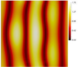
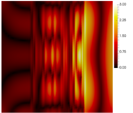
Figure 5.1: Metal cuboid $\tilde{\Sigma}_{1}$, the magnitude of $\operatorname{Re}(\hat{H})$ is plotted. Left: The $H$-field is $\operatorname{e}_{3}$-polarized and the plot shows values in the plane $x_{3}=0.5$. The analysis of both, (PC) and (HC) yields: transmission is possible. Right: The $H$-field is $\operatorname{e}_{2}$-polarized and the plot shows values in the plane $x_{2}=0.545$. Since the $H$-field is not parallel to $\operatorname{e}_{3}$, the analysis of (PC) and (HC) predicts that no transmission is possible. Inlet in the middle: Microstructure in the unit cube.

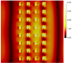
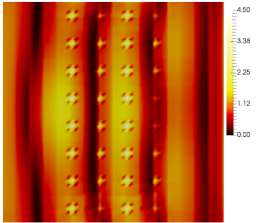
Figure 5.2: Test of numerical schemes for the metal cuboid $\tilde{\Sigma}_{1}$. We consider an $\operatorname{e}_{3}$-polarized incoming $H$-field and plot the solution in the plane $x_{3}=0.5$; the colors indicate the magnitude of the reference solution $\operatorname{Re}(H^{\eta})$ (left) and the zeroth order approximation $\operatorname{Re}(H^{0}_{\operatorname{HMM}})$ (right). Inlet in the center: Microsctructure in the unit cube with visualization plane in red.

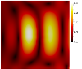
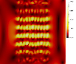
Figure 5.3: Metal cuboid $\tilde{\Sigma}_{2}$. We study an $\operatorname{e}_{3}$-polarized incident $H$-field and plot the magnitude of $\operatorname{Re}(\hat{H})$ (left) and $\operatorname{Re}(H^{\eta})$ (right) in the plane $x_{2}=0.545$. The analysis (PC) predicts transmission in this case, the analysis (HC) does not exclude transmission. Middle: Microstructure in the unit cube with visualization plane in red.

Instead of metal cylinders with circular base we study metal cuboids with square base, so that we do not have to deal with boundary approximations in our numerical method. We choose $\tilde{\Sigma}_{1}=(0.25,0.75)^{2}\times(0,1)$ and $\tilde{\Sigma}_{2}=(0,1)\times(0.25,0.75)^{2}$. Note that this choice influences the value of $\gamma$, but not the other results of Sections 3.1.1 and 3.1.2. Due to the symmetry of the microstructure, the effective material parameters are diagonal matrices with $a_{11}=a_{22}$, but with a different value $a_{33}$; see the analytical computations in Section 3.1.1. Up to numerical errors, we obtain the same structure for the computed approximative effective parameters.

Comparing the homogenized reference solution $\hat{H}$ for $\operatorname{e}_{2}$- and $\operatorname{e}_{3}$-polarized incoming waves for $\tilde{\Sigma}_{1}$ in Fig. 5.1, we observe that the $\operatorname{e}_{3}$-polarized wave is transmitted almost undisturbed through the meta-material. For the $\operatorname{e}_{2}$-polarization, however, the field intensity in $Q_{L}\coloneqq\{x\in G\colon x\leq 0.25\}$ is very low, corresponding to small transmission factors. This matches the analytical predictions of Section 3.1.1, which yields transmission only for $\operatorname{e}_{3}$-parallel $H$-fields. The same effect is predicted for high-contrast media by the analysis of Section 3.2.1.

The HMM can reproduce the behaviour of the homogenized and of the heterogeneous solution. For the comparison, we only consider the $\operatorname{e}_{3}$-polarized incoming wave in Fig. 5.2 and compare the zeroth order approximation $H_{\operatorname{HMM}}^{0}$ (right) to the (true) reference solution $H^{\eta}$ (left). Errors are still visible, but the qualitative agreement is good, even for the coarse mesh size of $h=h_{Y}=\sqrt{3}\cdot 1/16$ chosen for the HMM. In particular, the rather cheaply computable zeroth order approximation $H^{0}_{\operatorname{HMM}}$ can capture most of the important features of the true solution, even for inclusions of high-contrast. This clearly underlines the potential of the HMM. Moreover, Fig. 5.2 underlines the specific behaviour of $H^{\eta}$ in the inclusions $\tilde{\Sigma}_{\eta}$ for high-contrast media. As analyzed in Section 3.2.2, $H^{\eta}$ cannot be expected to vanish in the inclusions in the limit $\eta\to 0$ due to possible resonances; see [6]. We observe rather high field intensities in the inclusions; see also [37] for a slightly different inclusion geometry.

We also study the rotated metal cuboid $\tilde{\Sigma}_{2}$. In correspondence to the analysis of Section 3.1.2, we observe transmission for an $\operatorname{e}_{3}$-polarized incident wave; see Fig. 5.3. Note that the homogenized reference solution looks different to $\tilde{\Sigma}_{1}$ because of the rotation of the geometry, which is also reflected in the different structure and values of the reflection and transmission coefficients. The (true) reference solution in Fig. 5.4 shows the high field intensities in the metal cuboids induced by the high-contrast permittivity.

5.2 Metal plate $\Sigma_{3}$

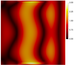
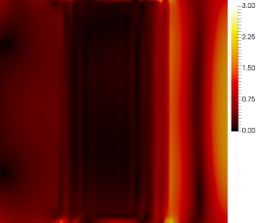
Figure 5.4: Metal plate $\Sigma_{3}$. The colors indicate the magnitude of $\operatorname{Re}(\hat{H})$ in the plane $x_{3}=0.5$. Left: The $H$-field is $\operatorname{e}_{3}$-polarized. The analysis (PC) predicts transmission, the analysis (HC) cannot exclude transmission. Right: The $H$-field is $\operatorname{e}_{2}$-polarized. The analysis (PC and HC) predicts that no transmission is possible.

As in Section 3.1.3, we choose a metal plate perpendicular to $\operatorname{e}_{2}$ of width $0.5$, i.e. $\Sigma_{3}=(0,1)\times(0.25,0.75)\times(0,1)$. Discretising the cell problems with mesh size $h_{Y}=\sqrt{3}\cdot 1/24$, we obtain—up to numerical errors—the effective material parameters as diagonal matrices with

$$\widehat{\varepsilon^{-1}} \approx\operatorname{diag}(10^{-4},0.5,10^{-4})\,,$$

$$\operatorname{Re}\hat{\mu} \approx\operatorname{diag}(0.228303,-0.044672,0.228303)\,.$$

Although we consider high-contrast media, this correspond astonishingly well to the analytical results for perfect conductors of Section 3.1.3: The structure of the matrices agrees and the non-zero value of $\widehat{\varepsilon^{-1}}=|Y\setminus\overline{\Sigma}|$ is as expected from the theory of perfect conductors. Due to the contributions of the inclusions, the values of $\mu_{\hom}$ are different from the case of perfect conductors.

Section 3.1.3 shows that, for perfect conductors, only an $H$-field polarized in $\operatorname{e}_{3}$-direction can be transmitted through the meta-material. Our numerical experiments allow a similar observation for high-contrast media in Fig. 5.4: The homogenized reference solution only shows a non-negligible intensity in the domain $Q_{L}=\{x\in G|x_{3}\leq 0.25\}$ left of the scatterer if the incident wave is polarized in $\operatorname{e}_{3}$ direction. Note that we have some reflections from the boundary in Fig. 5.4 since we do not use perfectly matched layers as boundary conditions. The observed transmission properties for high-contrast media are in accordance with the theory in Section 3.2: For an $\operatorname{e}_{3}$-polarized $H$-field as in the left figure, we cannot expect a (weak) convergence to zero. This corresponds to the observed non-trivial transmission. By contrast, in the right figure, the $H$-field is $\operatorname{e}_{2}$-polarized and no transmission can be observed. This corresponds to the analysis of Section 3.2.1, which shows that $H^{\eta}$ converges to zero, weakly in $L^{2}(Q_{M})$.

5.3 Air cuboid $\tilde{\Sigma}_{4}$

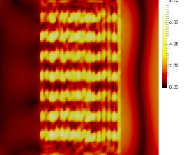
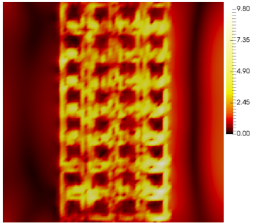
Figure 5.5: Metal block with holes. Left: The structure $\tilde{\Sigma}_{4}$, we plot the magnitude of $\operatorname{Re}(H^{\eta})$ in the plane $x_{3}=0.545$ for $\operatorname{e}_{3}$-polarized incoming $H$-field. The analysis (PC) predicts no transmission, the analysis (HC) cannot exclude transmission. Right: A geometry in which the cylinders $\tilde{\Sigma}_{4}$ are rotated in $\operatorname{e}_{3}$-direction. We plot the magnitude of $\operatorname{Re}(H^{\eta})$ in the plane $x_{3}=0.5$ for $\operatorname{e}_{3}$-polarized incoming $H$-field. Small pictures show the microstructures in the unit cube and the visualization planes in red.

As with the metal cylinder, we equip the air cylinder of Section 3.1.4 with a square base in order to have a geometry-fitting mesh. To be precise, we define the microstructure $\tilde{\Sigma}_{4}=(0,1)^{3}\setminus((0,1)\times(0.25,0.75)^{2})$. The effective permittivity $\widehat{\varepsilon^{-1}}$ vanishes almost identically for this setting; numerically we obtain only entries of order $10^{-5}$ for a discretisation of the corresponding cell problem with mesh size $h_{Y}=\sqrt{3}\cdot 1/24$. As discussed in Section 3.1.4, no transmission through this meta-material is expected for the high conductors. We observe the same for high-contrast media in Fig. 5.5: The (true) reference solution (almost) vanishes in the left part $Q_{L}$ in all situations. Here, we only depict $\operatorname{e}_{3}$-polarized incident waves, once for $\tilde{\Sigma}_{4}$ as described and once for the rotated air cuboid with main axis in $\operatorname{e}_{3}$-direction (this is the setting of Section 3.1.1 with interchanged roles of metal and air). Note that inside the microstructure, high intensities and amplitudes of the $H^{\eta}$-field occur due to resonances in the high-contrast medium.

Conclusion

We analyzed the transmission properties of meta-materials consisting of perfect conductors or high-contrast materials. Depending on the geometry of the microstructure, certain entries in the effective material parameters vanish, which induces that also certain components of the solution vanish. This influences the transmission properties of the material. Transmission is possible only for certain polarizations of the incoming wave. For perfect conductors, we derived closed formulas for the reflection and transmission coefficients. Using the Heterogeneous Multiscale Method, the homogenized solution as well as some features of the exact solution can be approximated on rather coarse meshes and, in particular, with a cost that is independent of the periodicity length. Our numerical experiments of three representative geometries with high-contrast materials confirm the theoretical predictions of their transmission properties.

References

- [1] A. Abdulle. On a priori error analysis of fully discrete heterogeneous multiscale FEM. Multiscale Model. Simul., 4:447–459, 2005.
- [2] P. Bastian, M. Blatt, A. Dedner, C. Engwer, R. Klöfkorn, R. Kornhuber, M. Ohlberger, and O. Sander. A generic grid interface for parallel and adaptive scientific computing. II. Implementation and tests in DUNE. Computing, 82(2-3):121–138, 2008.
- [3] P. Bastian, M. Blatt, A. Dedner, C. Engwer, R. Klöfkorn, M. Ohlberger, and O. Sander. A generic grid interface for parallel and adaptive scientific computing. I. Abstract framework. Computing, 82(2-3):103–119, 2008.
- [4] A. Bonito, J.-L. Guermond, and F. Luddens. Regularity of the Maxwell equations in heterogeneous media and Lipschitz domains. J. Math. Anal. Appl., 408(2):498–512, 2013.
- [5] G. Bouchitté and C. Bourel. Multiscale nanorod metamaterials and realizable permittivity tensors. Commun. Comput. Phys., 11(2):489–507, 2012.
- [6] G. Bouchitté, C. Bourel, and D. Felbacq. Homogenization of the 3D Maxwell system near resonances and artificial magnetism. C. R. Math. Acad. Sci. Paris, 347(9–10):571–576, 2009.
- [7] G. Bouchitté, C. Bourel, and D. Felbacq. Homogenization near resonances and artificial magnetism in three dimensional dielectric metamaterials. Arch. Ration. Mech. Anal., 225(3):1233–1277, 2017.
- [8] G. Bouchitté and D. Felbacq. Homogenization near resonances and artificial magnetism from dielectrics. C. R. Math. Acad. Sci. Paris, 339(5):377–382, 2004.
- [9] G. Bouchitté and D. Felbacq. Homogenization of a wire photonic crystal: the case of small volume fraction. SIAM J. Appl. Math., 66(6):2061–2084, 2006.
- [10] G. Bouchitté and B. Schweizer. Homogenization of Maxwell’s equations in a split ring geometry. Multiscale Model. Simul., 8(3):717–750, 2010.
- [11] G. Bouchitté and B. Schweizer. Plasmonic waves allow perfect transmission through sub-wavelength metallic gratings. Netw. Heterog. Media, 8(4):857–878, 2013.
- [12] L. Cao, Y. Zhang, W. Allegretto, and Y. Lin. Multiscale asymptotic method for Maxwell’s equations in composite materials. SIAM J. Numer. Anal., 47(6):4257–4289, 2010.
- [13] K. Cherednichenko and S. Cooper. Homogenization of the system of high-contrast Maxwell equations. Mathematika, 61(2):475–500, 2015.
- [14] V. T. Chu and V. H. Hoang. High-dimensional finite elements for multiscale maxwell-type equations. IMA Journal of Numerical Analysis, 38(1):227–270, 2018.
- [15] E. T. Chung and Y. Li. Adaptive generalized multiscale finite element methods for H(curl)-elliptic problems with heterogeneous coefficients. J. Comput. Appl. Math., 345:357–373, 2019.
- [16] P. Ciarlet Jr., S. Fliss, and C. Stohrer. On the approximation of electromagnetic fields by edge finite elements. Part 2: A heterogeneous multiscale method for Maxwell’s equations. Comput. Math. Appl., 73(9):1900–1919, 2017.
- [17] M. Costabel and M. Dauge. Singularities of electromagnetic fields in polyhedral domains. Arch. Ration. Mech. Anal., 151:221–276, 2000.
- [18] M. Costabel, M. Dauge, and S. Nicaise. Singularities of Maxwell interface problems. M2AN Math. Model. Numer. Anal., 33(3):627–649, 1999.
- [19] W. E and B. Engquist. The heterogeneous multiscale methods. Commun. Math. Sci., 1(1):87–132, 2003.
- [20] W. E and B. Engquist. The heterogeneous multi-scale method for homogenization problems. In Multiscale methods in science and engineering, volume 44 of Lect. Notes Comput. Sci. Eng., pages 89–110. Springer, Berlin, 2005.
- [21] W. E, P. Ming, and P. Zhang. Analysis of the heterogeneous multiscale method for elliptic homogenization problems. J. Amer. Math. Soc., 18:121–156, 2005.
- [22] A. Efros and A. Pokrovsky. Dielectroc photonic crystal as medium with negative electric permittivity and magnetic permeability. Solid State Communications, 129(10):643–647, 2004.
- [23] D. Felbacq and G. Bouchitté. Homogenization of a set of parallel fibres. Waves Random Media, 7(2):245–256, 1997.
- [24] D. Gallistl, P. Henning, and B. Verfürth. Numerical homogenization of H(curl)-problems. SIAM J. Numer. Anal., 56(3):1570–1596, 2018.
- [25] P. Henning, M. Ohlberger, and B. Verfürth. A new Heterogeneous Multiscale Method for time-harmonic Maxwell’s equations. SIAM J. Numer. Anal., 54(6):3493–3522, 2016.
- [26] M. Hochbruck and C. Stohrer. Finite element heterogeneous multiscale method for time-dependent Maxwell’s equations. In M. Bittencourt, N. Dumont, and J. Hesthaven, editors, Spectral and High Order Methods for Partial Differential Equations ICOSAHOM 2016, volume 119 of Lect. Notes Comput. Sci. Eng., pages 269–281. Springer, Cham, 2017.
- [27] A. Lamacz and B. Schweizer. A negative index meta-material for Maxwell’s equations. SIAM J. Math. Anal., 48(6):4155–4174, 2016.
- [28] R. Lipton and B. Schweizer. Effective Maxwell’s equations for perfectly conducting split ring resonators. Arch. Ration. Mech. Anal., 229(3):1197–1221, 2018.
- [29] C. Luo, S. G. Johnson, J. Joannopolous, and J. Pendry. All-angle negative refraction without negative effective index. Phys. Rev. B, 65(2001104), 2002.
- [30] R. Milk and F. Schindler. dune-gdt, 2015. dx.doi.org/10.5281/zenodo.35389.
- [31] P. Monk. Finite element methods for Maxwell’s equations. Numerical Mathematics and Scientific Computation. Oxford University Press, New York, 2003.
- [32] M. Ohlberger. A posteriori error estimates for the heterogeneous multiscale finite element method for elliptic homogenization problems. Multiscale Model. Simul., 4(1):88–114 (electronic), 2005.
- [33] M. Ohlberger and B. Verfürth. A new Heterogeneous Multiscale Method for the Helmholtz equation with high contrast. Mulitscale Model. Simul., 16(1):385–411, 2018.
- [34] A. Pokrovsky and A. Efros. Diffraction theory and focusing of light by a slab of left-handed material. Physica B: Condensed Matter, 338(1-4):333–337, 2003. Proceedings of the Sixth International Conference on Electrical Transport and Optical Properties of Inhomogeneous Media.
- [35] B. Schweizer. Resonance meets homogenization: construction of meta-materials with astonishing properties. Jahresber. Dtsch. Math.-Ver., 119(1):31–51, 2017.
- [36] B. Schweizer and M. Urban. Effective Maxwell’s equations in general periodic microstructures. Applicable Analysis, 97(13):2210–2230, 2017.
- [37] B. Verfürth. Heterogeneous Multiscale Method for the Maxwell equations with high contrast. arXiv preprint, 2017.