Coherent Compton scattering from hydrogen and helium atoms

Abstract

We develop an approach to describing coherent Compton scattering of photons in the keV energy range from hydrogen and helium atoms based on a relativistic version of the AA-approximation within the standard perturbative S-matrix formalism. The resulting formulas for the cross section take into account the effects of the electron boundness and correctly reproduce the behavior of the cross section at large photon energies, where it goes to Thomson formula, which coincides with the Klein-Nishina-Tamm formula for the cross section in the non-relativistic limit.

• September 2018

1 Introduction

Compton scattering is (quasi)elastic scattering of photons by electrons, which takes place for both free and bound electrons and is well studied in the former case. The cross section of this process in the case of free electrons is given by the famous Klein-Nishina-Tamm formula [1, 2]. However, Compton scattering by bound electrons is much less studied both experimentally and theoretically.

It is a common knowledge that the interaction of photons with atoms at energies above their ionization energy and below 1 MeV goes due to two processes. The first one is photoelectric emission, which takes place only for bound electrons. At the energies of the order of the electron binding energy photoelectric emission is the dominating process with a large cross section proportional to Bohr’s radius squared. However, the cross section of this process rapidly goes down with increasing photon energy and at larger energies the process of Compton scattering becomes the dominating one. For light atoms the boundary lies in the keV energy range.

In the perturbative approach, Compton scattering is described by the second Born approximation [3, 4]. In the non-relativistic description of the process, as well as in the relativistic one, exact Green’s function entering the amplitude of the process involves the summation over the intermediate electron eigenstates in the field of a nucleus. This summation is the most difficult problem in the calculations, which makes it necessary to develop various approximate summation methods. For example, this problem is discussed in detail in book [5]. For non-relativistic processes with relatively small energy transferred by a photon to the atom, the sum is dominated by the electron states from the continuum in the Coulomb field of the nucleus, which are often replaced by plane waves. This is the so-called non-relativistic AA-approximation.

In the relativistic description a similar approximation consists in replacing exact Green’s function of electron in the external Coulomb field by free Green’s function of electron. Then, in the perturbative S-matrix formalism, Compton scattering from bound electrons can be viewed as photoelectric emission of an off-shell electron, which then emits a photon. It looks as if the electron absorbs a part of the photon energy and increases its mass, thus transforming the process to photoelectric emission of a heavier electron by a less energetic photon, which leads to an increase of the cross section. This picture gives reason to expect that the cross section of Compton scattering from bound electrons should include a term that behaves similar to the cross section of photoelectric emission, takes into account the effects of boundness and falls off with growing energy. However, Compton scattering can take place also at free electrons, and with the growth of the photon energy the electrons in the atoms can be approximately considered to be free. For this reason the cross section of Compton scattering from bound electrons in the limit of high photon energy should be given by the Klein-Nishina-Tamm formula somehow modified by the electron wave function. However, this description is used for all photon energies in the majority of papers dealing with Compton scattering by bound electrons [6, 7, 8].

Since the ionization energy is different for the electrons of different shells, Compton scattering by bound electrons is a coherent process only for the electrons of the same shell. Here we develop an approach to describing coherent Compton scattering of photons by the electrons bound in hydrogen and helium atoms, which have only one electron shell. The generalization to atoms with a larger number of electron shells is straightforward and consists in summing the cross sections of Compton scattering from the electrons of different shells.

The experimental situation in Compton scattering looks as follows. Nowadays there is a great demand for coincidental experiments, where the angles and energies of the outgoing electron and photon (more precisely, of the ion-residue) are measured simultaneously. Such experiments allow one to get a deeper insight into the picture of the momentum distributions in target atoms and, probably, to expand and to complement the information obtained from other coincidental experiments, for example, from EIS (electron impulse approximation) [9, 10]. However, the differential cross section measured in such experiments is 5-7 orders of magnitude lass than the typical cross section of photoelectric emission, which is a serious problem. Nevertheless, such experiments are carried out (see, for example, [11, 12]) and, to the best of our knowledge, new experiments are planned. It is worth noting that such experiments usually deal with photons in the energy range of several keV.

In the present paper we consider Compton scattering by electrons in the ground states of hydrogen and helium atoms in a relativistic version of the AA-approximation. The process of Compton scattering by bound electrons is characterized by thee parameters of the dimension of energy: the bound state energy $\varepsilon<0$, the photon energy $\omega_{1}$, and the electron mass $m$. We will consider the process in the most interesting energy range of several keV, where the dimensionless quantities $|\varepsilon|/\omega_{1}\ll 1$ and $\omega_{1}/m\ll 1$ can be neglected. However, the ratio of these quantities $m|\varepsilon|/\omega_{1}^{2}$ can be of the order of unity and should be kept in the formulas. It turns out that the corrections due to this ratio are significant and take into account the electron boundness.

The approach is based on the standard S-matrix formalism, which seems to be most suitable for describing this process. This is due to the fact that the standard perturbative S-matrix formalism naturally considers this process as photoelectric emission of off-shell electrons, which then emit a photon and return to the mass shell. Since the process takes place in the Coulomb field of the nucleus, it turns out to be convenient to use the S-matrix formalism in the Furry representation.

Throughout the paper we will follow the conventions of textbook [3] and use the Gauss system of units adopted in atomic physics, as well as the relation $\hbar=c=1.$

2 Theory

2.1 Compton scattering by hydrogen atoms

In order to make the presentation clearer, first we will calculate Compton scattering by electrons in the ground state of hydrogen atoms in the second order of perturbation theory. Compton scattering from electrons in helium atoms differs from it only in two aspects that will be discussed later. The relevant part of the second order S-matrix in the Furry representation looks like

$$S^{(2)}=i\,e^{2}N\int\bar{\psi}(x_{2})\hat{A}(x_{2})S_{e}(x_{2},x_{1})\hat{A}(x_{1})\psi(x_{1})dx_{1}dx_{2},$$ (1)

where N denotes the normal ordering of the operators, $\hat{A}(x)=\gamma^{\mu}A_{\mu}(x)$, and $S_{e}(x_{2},x_{1})$ is Green’s function of electron in an external Coulomb field. The field $\psi(x)$ should also be expanded in the electron eigenstates in this external field, and $\bar{\psi}(x_{2})$ denotes the Dirac conjugate of $\psi(x_{2})$.

The processes of scattering, corresponding to this S-matrix term, are represented by the diagrams depicted in Figure 1.

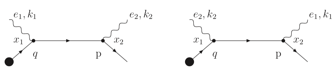
Figure 1: Scattering diagrams.

Here the incoming photon is the one with the polarization and momentum $e_{1},k_{1}$ and the scattered photon is the one with the polarization and momentum $e_{2},k_{2}$. Below we will denote the photon energies $k_{1}^{0}=\omega_{1}$ and $k_{2}^{0}=\omega_{2}$.

As we have explained in the Introduction, we will use the following approximation: we will assume that the incoming electron line marked by the filled circle corresponds to the electron ground state wave function $e^{-i(m+\varepsilon)t_{1}}\psi_{0}(\vec{x}_{1})$ with the energy $\varepsilon=-13.62\,$eV in the Coulomb field of proton, whereas the two other electron lines correspond to Green’s function $S(x_{2}-x_{1})$ of the free electron field and to the electron plane wave with momentum $\vec{p}$. Substituting the corresponding wave and Green’s functions into (1), integrating with respect to $x_{1}$ and $x_{2}$, denoting $m+\varepsilon=q^{0}$ and dropping the delta function $2\pi\delta(k_{1}^{0}+q^{0}-k_{2}^{0}-p^{0})$ of energy conservation, we get the following amplitude of the process:

$$M = -4\pi e^{2}e_{2}^{*\mu}e_{1}^{\nu}\left(\bar{u}(p)Q_{\mu\nu}\tilde{\psi}_{0}(\vec{q})\right)$$ (2)

$$Q_{\mu\nu} = \gamma_{\mu}\frac{\hat{q}+\hat{k}_{1}+m}{(q+k_{1})^{2}-m^{2}}\gamma_{\nu}+\gamma_{\nu}\frac{\hat{q}-\hat{k}_{2}+m}{(q-k_{2})^{2}-m^{2}}\gamma_{\mu},$$ (3)

where $\hat{q}=\gamma_{\mu}q^{\mu},\,\,q=(m+\varepsilon,\vec{q}),\,\,\vec{q}=\vec{p}+\vec{k}_{2}-\vec{k}_{1}$, $\bar{u}(p)$ is the Dirac conjugate of the spinor $u(p)$, and the Fourier transform of the wave function is defined as

$$\tilde{\psi}_{0}(\vec{q})=\int e^{-i\vec{q}\vec{x}}\psi_{0}(\vec{x})d\vec{x}.$$ (4)

This amplitude implies that we have to use a relativistic wave function of the hydrogen ground state $\psi_{0}(\vec{x})$, which is a Dirac spinor. However, for our purpose it is sufficient to take the non-relativistic hydrogen wave function with the first relativistic correction. Thus, the wave function $\psi_{0}(\vec{x})$ will be taken in the form (see [3], §57)

$$\psi_{0}(\vec{x})=\left(1-\frac{i\gamma^{0}\vec{\gamma}\vec{\nabla}}{2m}\right)\frac{u}{\sqrt{2m}}\psi_{nr}(\vec{x}),$$ (5)

where $u$ is a solution of the Dirac equation for the electron at rest normalized by the condition $\bar{u}u=2m,$ and $\psi_{nr}(\vec{x})$ is the non-relativistic wave function of the ground state of the hydrogen atom. The wave function $\psi_{0}(\vec{x})$ is normalized to unity up to a term of the order of $|\varepsilon|/m$, which is negligibly small. Such terms will be always dropped in our calculations.

Now to find the cross section of the Compton scattering process, first we have to calculate the squared amplitude. According to the general rules, the common factor in front of the squared amplitude will be

$$2\pi\delta(k_{1}^{0}+q^{0}-k_{2}^{0}-p^{0}).$$ (6)

Here we will calculate the cross section of the process with unpolarized particles. To this end, we have to average the squared amplitude over the polarizations of the incoming particles and to sum it over the polarizations of the outgoing particles. The summations over the polarizations of the photons and the outgoing electron are standard. The summation over the polarizations of the incoming bound electron gives

$$\left(1+\frac{\gamma^{0}\vec{\gamma}\vec{q}}{2m}\right)\frac{\sum_{s}u^{s}\bar{u}^{s}}{{2m}}\left(1-\frac{\gamma^{0}\vec{\gamma}\vec{q}}{2m}\right)=\left(1+\frac{\gamma^{0}\vec{\gamma}\vec{q}}{2m}\right)\frac{\gamma^{0}+1}{{2}}\left(1-\frac{\gamma^{0}\vec{\gamma}\vec{q}}{2m}\right)$$

$$= \frac{1}{2m}\left((\hat{q}+m)+\gamma^{0}(\frac{\vec{q}^{\,2}}{4m}-\varepsilon)-\frac{\vec{q}^{\,2}}{4m}\right).$$

The terms $\frac{\vec{q}^{\,2}}{m}$ and $|\varepsilon|$ are negligibly small compared to $m$ and can be dropped. This means that the squared amplitude of Compton scattering from electrons bound in hydrogen atoms averaged over the polarizations of the incoming photon and electron and summed over the polarizations of the outgoing particles can be written as

$$\overline{{|M|}^{\,2}}=\frac{16\pi^{2}e^{4}}{8m}|\tilde{\psi}_{nr}(\vec{q})|^{2}tr\left((\hat{q}+\hat{k}_{1}-\hat{k}_{2}+m)Q_{\mu\nu}(\hat{q}+m)Q^{\mu\nu}\right),$$ (7)

and in calculating the numerator of this amplitude we can put $q^{\,2}=m^{2}$, i.e. put the incoming electron on the mass shell, which is equivalent to neglecting the terms $\frac{\vec{q}^{\,2}}{m}$ and $|\varepsilon|$ everywhere in the numerator. The validity of this approximation has been checked by direct calculations of the squared amplitude, which turned out to be rather complicated.

It is convenient to represent the trace in formula (7) as [4]

$$tr\left((\hat{q}+\hat{k}_{1}-\hat{k}_{2}+m)Q_{\mu\nu}(\hat{q}+m)Q^{\mu\nu}\right)=32F,$$ (8)

where $F$ is a scalar function of the momenta $q,k_{1},k_{2}$ and the electron mass $m$. In the approximation we use this function is given by the standard expression, which can be found in §86 of textbook [3]:

$$F = \left(\frac{m^{2}}{(q+k_{1})^{2}-m^{2}}+\frac{m^{2}}{(q-k_{2})^{2}-m^{2}}\right)^{2}$$

$$+ \left(\frac{m^{2}}{(q+k_{1})^{2}-m^{2}}+\frac{m^{2}}{(q-k_{2})^{2}-m^{2}}\right)$$

$$- \frac{1}{4}\left(\frac{(q+k_{1})^{2}-m^{2}}{(q-k_{2})^{2}-m^{2}}+\frac{(q-k_{2})^{2}-m^{2}}{(q+k_{1})^{2}-m^{2}}\right).$$

Now we can write the following expression for the differential cross section of Compton scattering from hydrogen atom

$$d\sigma=2\pi\delta(k_{1}^{0}+q^{0}-k_{2}^{0}-p^{0})\frac{32\pi^{2}e^{4}}{m\omega_{1}}F|\tilde{\psi}_{nr}(\vec{q})|^{2}\frac{d\vec{k}_{2}}{(2\pi)^{3}2k_{2}^{0}}\,\frac{d\vec{p}}{(2\pi)^{3}2p^{0}},$$ (10)

where $\vec{q}=\vec{p}+\vec{k}_{2}-\vec{k}_{1}$. The fully differential cross section of the process is obtained by integrating this expression with respect to $|\vec{k}_{2}|$:

$$\frac{d\sigma}{d\Omega_{\vec{k}_{2}}d\Omega_{e}dE_{e}}=\frac{r_{0}^{2}m|\vec{p}|}{4\pi^{3}}\frac{\omega_{2}}{\omega_{1}}F\ |\tilde{\psi}_{nr}(\vec{q})|^{2}.$$ (11)

Here $r_{0}=\frac{e^{2}}{m}$ is the classical radius of the electron, $E_{e}$ is kinetic energy of the scattered electron and $\omega_{2}=\omega_{1}+\varepsilon-\frac{\vec{p}^{2}}{2m}$ is defined by energy conservation.

Now we have to calculate the scalar function $F$ in our approximation. To this end, let us consider energy-momentum conservation for the scattering process:

$$q+k_{1}-k_{2}=p.$$ (12)

Squaring both sides of the equation gives

$$2m\varepsilon-\vec{q}^{\,2}+\varepsilon^{2}+2(m+\varepsilon)(\omega_{1}-\omega_{2})-2\vec{q}(\vec{k}_{1}-\vec{k}_{2})-2\omega_{1}\omega_{2}+2\omega_{1}\omega_{2}\cos\theta=0,$$ (13)

where $\theta$ is the angle between the momenta $\vec{k}_{1}$ and $\vec{k}_{2}$ of the incoming and the outgoing photons, and we have dropped the term $\varepsilon^{2}$. As we have already explained in the Introduction, we will always assume that the conditions $|\varepsilon|/\omega_{1}\ll 1$ and $\omega_{1}/m\ll 1$ are fulfilled, which means that the photon energy is in the keV energy range. Then dividing equation (13) by $2\omega_{1}\omega_{2}$ and neglecting the terms $|\varepsilon|/\omega_{1},\,|\varepsilon|/\omega_{2}$ and $\varepsilon^{2}/\omega_{1}\omega_{2}$, we get

$$\frac{m}{\omega_{2}}-\frac{m}{\omega_{1}}+\frac{m\varepsilon}{\omega_{1}\omega_{2}}-\frac{\vec{q}^{\,2}}{2\omega_{1}\omega_{2}}-\frac{\vec{q}(\vec{k}_{1}-\vec{k}_{2})}{\omega_{1}\omega_{2}}=1-\cos\theta.$$ (14)

We emphasize that the terms in this equation containing $\varepsilon$ and $\vec{q}$ can be of the order of unity and cannot be dropped here, as well as in eq. (13).

Now we need to find the factor $F$ in the approximation we use. To this end, we have to calculate the denominators in expression (2.1) for $F$. The first denominator is

$$(q+k_{1})^{2}-m^{2}\simeq 2m\omega_{1}-2\vec{q}\vec{k}_{1}+2m\varepsilon-\vec{q}^{\,2},$$ (15)

where we have dropped the term $\varepsilon^{2}$. Unlike the numerator, in the denominator we cannot neglect the small terms $\vec{q}^{\,2}$ and $2m|\varepsilon|$, because the deviation of the virtual electrons from the mass shell is very small. Then we get

$$\frac{m^{2}}{(q+k_{1})^{2}-m^{2}}\simeq\frac{1}{2}\left(\frac{m}{\omega_{1}}+\frac{\vec{q}\vec{k}_{1}}{\omega_{1}^{2}}+\frac{m\varepsilon}{\omega_{1}^{2}}+\frac{\vec{q}^{\,2}}{2\omega_{1}^{2}}\right).$$ (16)

Analogously, we find

$$\frac{m^{2}}{(q-k_{2})^{2}-m^{2}}\simeq-\frac{1}{2}\left(\frac{m}{\omega_{2}}+\frac{\vec{q}\vec{k}_{2}}{\omega_{2}^{2}}+\frac{m\varepsilon}{\omega_{2}^{2}}-\frac{\vec{q}^{\,2}}{2\omega_{2}^{2}}\right).$$ (17)

The first terms in the right hand sides of formulas (16), (17) are the standard terms for Compton scattering from electrons at rest, whereas the other terms are the corrections due to the electrons being bound in a hydrogen atom.

Thus, the expression in the first bracket in formula (2.1) turns out to be

$$\frac{m^{2}}{(q+k_{1})^{2}-m^{2}}+\frac{m^{2}}{(q-k_{2})^{2}-m^{2}}\simeq$$ (18)

$$\frac{1}{2}\left(\frac{m}{\omega_{1}}-\frac{m}{\omega_{2}}-\frac{m\varepsilon}{\omega_{1}^{2}}-\frac{m\varepsilon}{\omega_{2}^{2}}+\frac{\vec{q}^{\,2}}{2\omega_{1}^{2}}+\frac{\vec{q}^{\,2}}{2\omega_{2}^{2}}+\frac{\vec{q}\vec{k}_{1}}{\omega_{1}^{2}}-\frac{\vec{q}\vec{k}_{2}}{\omega_{2}^{2}}\right).$$

Here, with the accuracy up to terms of the order of $|\varepsilon|/\omega_{1}$ and $\omega_{1}/m$, we can replace

$$\frac{\vec{q}\vec{k}_{1}}{\omega_{1}^{2}}-\frac{\vec{q}\vec{k}_{2}}{\omega_{2}^{2}} \rightarrow \frac{\vec{q}(\vec{k}_{1}-\vec{k}_{2})}{\omega_{1}\omega_{2}},$$ (19)

$$-\frac{m\varepsilon}{\omega_{2}^{2}}+\frac{\vec{q}^{\,2}}{2\omega_{2}^{2}} \rightarrow -\frac{m\varepsilon}{\omega_{1}\omega_{2}}+\frac{\vec{q}^{\,2}}{2\omega_{1}\omega_{2}}$$ (20)

and then use relation (14) for the photon energies. As a result, we get

$$\frac{m^{2}}{(q+k_{1})^{2}-m^{2}}+\frac{m^{2}}{(q-k_{2})^{2}-m^{2}}\simeq\frac{1}{2}\left(-\frac{m\varepsilon}{\omega_{1}^{2}}+\frac{\vec{q}^{\,2}}{2\omega_{1}^{2}}-(1-cos^{2}\theta)\right).$$ (21)

In a similar way one can find that the third term in formula (2.1) is reduced, up to terms of the order of $|\varepsilon|/m$, to

$$-\frac{1}{4}\left(\frac{(q+k_{1})^{2}-m^{2}}{(q-k_{2})^{2}-m^{2}}+\frac{(q-k_{2})^{2}-m^{2}}{(q+k_{1})^{2}-m^{2}}\right)\approx\frac{1}{4}\left(\frac{\omega_{1}}{\omega_{2}}+\frac{\omega_{2}}{\omega_{1}}\right),$$ (22)

which, up to terms of the order of $(\varepsilon/\omega_{1})^{2}$, is equal to $1/2$.

Based on these results, it is not difficult to find an expression for $F$ in our approximation:

$$F=\frac{1}{4}\left(\left(-\frac{m\varepsilon}{\omega_{1}^{2}}+\frac{\vec{q}^{\,2}}{2\omega_{1}^{2}}\right)^{2}+2\left(-\frac{m\varepsilon}{\omega_{1}^{2}}+\frac{\vec{q}^{\,2}}{2\omega_{1}^{2}}\right)\cos\theta+(1+\cos^{2}\theta)\right).$$ (23)

Then the fully differential cross section (FDCS) can be written as

$$\frac{d^{3}\sigma}{d\Omega_{\vec{k}_{2}}d\Omega_{e}dE_{e}}=\frac{r_{0}^{2}m|\vec{p}|}{2(2\pi)^{3}}\times$$

$$\left(\left(-\frac{m\varepsilon}{\omega_{1}^{2}}+\frac{\vec{q}^{\,2}}{2\omega_{1}^{2}}\right)^{2}+2\left(-\frac{m\varepsilon}{\omega_{1}^{2}}+\frac{\vec{q}^{\,2}}{2\omega_{1}^{2}}\right)\cos\theta+(1+\cos^{2}\theta)\right)|\tilde{\psi}_{nr}(\vec{q})|^{2},$$ (24)

where $\vec{q}=\vec{p}+\vec{k}_{2}-\vec{k}_{1}$ and we have put the ratio of the photon energies equal to unity in the approximation we use. We see that the fully differential cross section depends on the squared wave function of the electron. Thus, measuring this fully differential cross section can give information on the momentum distribution of the electrons in hydrogen atom, which is to be compared with the distribution given by the electron wave function of the ground state.

It is interesting to find the single differential cross section (SDCS) $\frac{d\sigma}{d\Omega_{\vec{k}_{2}}}$, which generalizes the Klein-Nishina-Tamm formula to the case of the scattering from bound electrons in the energy range under consideration and could be obtained by integrating formula (2.1) with respect to $\vec{p}$. However, the straightforward integration turns out to be inconvenient. To find this differential cross section we return to formula (10) and identically rewrite it as follows:

$$d\sigma=\frac{32\pi^{2}e^{4}}{m\omega_{1}}\frac{d\vec{k}_{2}}{(2\pi)^{3}2k_{2}^{0}}\,\frac{d\vec{p}}{(2\pi)^{3}2p^{0}}\times$$

$$\int|\tilde{\psi}_{nr}(\vec{q})|^{2}\frac{d\vec{q}}{(2\pi)^{3}}\,(2\pi)^{4}\delta^{(4)}(k_{1}+q-k_{2}-p)F,$$ (25)

where the delta function is now four-dimensional, i.e. it includes the delta function of the particle momenta $\delta(\vec{k}_{1}+\vec{q}-\vec{k}_{2}-\vec{p})$. We see that the differential cross section looks like the cross section of Compton scattering from an off-shell electron with four-momentum $q=(m+\varepsilon,\vec{q})$ averaged over the momenta with the weight $|\tilde{\psi}_{nr}(\vec{q})|^{2}/{(2\pi)^{3}}$.

It is convenient to write SDCS in the form

$$\frac{d\sigma}{d\Omega_{\vec{k}_{2}}}=\frac{2e^{4}}{m\omega_{1}}\int\frac{d\vec{q}}{(2\pi)^{3}}|\tilde{\psi}_{nr}(\vec{q})|^{2}\int\int\frac{\omega_{2}d\omega_{2}d\vec{p}}{p^{0}}\delta^{(4)}(q+k_{1}-k_{2}-p)F.$$ (26)

The integration with respect to $\vec{p}$ is done with the help of the delta function $\delta(\vec{q}+\vec{k}_{1}-\vec{k}_{2}-\vec{p})$, which gives $\vec{p}=\vec{q}+\vec{k}_{1}-\vec{k}_{2}$. Since $\vec{p}^{2}/m^{2}\ll 1$, we can put $p^{0}=m$ in the denominator and get the following expression for the cross section

$$\frac{d\sigma}{d\Omega_{\vec{k}_{2}}}=\frac{2r_{0}^{2}}{\omega_{1}}\int\frac{d\vec{q}}{(2\pi)^{3}}|\tilde{\psi}_{nr}(\vec{q})|^{2}\int\omega_{2}d\omega_{2}\delta(\omega_{1}+\varepsilon-\omega_{2}-\frac{\vec{p}^{\,2}}{2m})F,$$ (27)

where $r_{0}=e^{2}/m$ is the classical radius of the electron.

The integration with respect to $\omega_{2}$ is done with the help of the delta function of energy conservation. It results in relation (14) for the photon energies and in the multiplication of the function $F$ by a factor, which differs from unity in terms of the order of $\omega_{1}/m$ and can be dropped.

It remains to integrate the cross section with respect to $\vec{q}$, i.e. to average over the momentum of the bound electron, as well as to average over the momentum the other relations. Averaging relation (14) gives

$$\frac{m}{\omega_{2}}-\frac{m}{\omega_{1}}+\frac{2m\varepsilon}{\omega_{1}\omega_{2}}=1-\cos\theta,$$ (28)

or, equivalently,

$${\omega_{2}}=\frac{\omega_{1}-2|\varepsilon|}{1+\frac{\omega_{1}}{m}(1-\cos\theta)},$$ (29)

which generalizes the well-known formula for Compton scattering from free electrons to the case of bound electrons. However, unlike in the case of free electrons, since the energy of the scattered photons ${\omega_{2}}$ is found by averaging formula (14), it should be viewed as the mean energy of the scattered photon beam. The broadening of the energy spectrum of the scattered photons due to the motion of electrons in hydrogen atoms is given by

$$\sqrt{\left<\left(\frac{\vec{q}^{\,2}}{2m}+\frac{\vec{q}(\vec{k}_{1}-\vec{k}_{2})}{m}\right)^{2}\right>-\left<\frac{\vec{q}^{\,2}}{2m}+\frac{\vec{q}(\vec{k}_{1}-\vec{k}_{2})}{m}\right>^{2}}\simeq\sqrt{\varepsilon^{2}(\beta-1)}=2|\varepsilon|,$$

where $\beta=\langle(\vec{q}^{\,2})^{2}\rangle/\langle\vec{q}^{\,2}\rangle^{2}=5$ is a parameter that depends only on the wave function of the electrons in hydrogen atom.

Similarly, averaging the factor $F$ gives

$$\overline{F}=\frac{1}{4}\left((3+\beta)\left(\frac{m\varepsilon}{\omega_{1}^{2}}\right)^{2}-4\left(\frac{m\varepsilon}{\omega_{1}^{2}}\right)\cos\theta+(1+\cos^{2}\theta)\right).$$ (30)

Correspondingly, the differential cross section is found to be

$$\frac{d\sigma}{d\Omega_{\vec{k}_{2}}}=\frac{r_{0}^{2}}{2}\left(8\left(\frac{m\varepsilon}{\omega_{1}^{2}}\right)^{2}+4\left(\frac{m|\varepsilon|}{\omega_{1}^{2}}\right)\cos\theta+(1+\cos^{2}\theta)\right),$$ (31)

where we have put $\beta=5.$ The first term in the brackets can be brought to the form

$$4{r_{0}^{2}}\left(\frac{m\varepsilon}{\omega_{1}^{2}}\right)^{2}=4{a_{0}^{2}}\left(\frac{\varepsilon}{\omega_{1}}\right)^{4},$$

where $a_{0}=1/me^{2}$ is Bohr’s radius. The formula is somewhat similar to the cross section of photoelectric emission due to its dependence on the ratio of the binding energy to the photon energy and to the factor $a_{0}^{2}$. This term takes into account the boundness of the electrons in hydrogen atoms. The term $\frac{r_{0}^{2}}{2}\left(1+\cos^{2}\theta\right)$ corresponds to Thomson scattering, to which Compton scattering from free electrons is reduced in the energy range under consideration, and the term $2r_{0}^{2}\left(\frac{m|\varepsilon|}{\omega_{1}^{2}}\right)\cos\theta=2r_{0}a_{0}\left(\frac{\varepsilon}{\omega_{1}}\right)^{2}\cos\theta$ can be considered as an interference term.

It is necessary to note that the description of the outgoing electron in the Coulomb field by the plane wave can fail at small momenta of the electron. This is not critical for the differential cross section given by formula (31), where we have integrated over this energy range. However, in formula (2.1) for the fully differential cross section it can be of importance.

This flaw can be amended as follows. We observe that the squared absolute value of the Fourier transform of the electron ground state wave function enters the expression for the fully differential cross section as a factor. The Fourier transform can be viewed as the matrix element

$$\tilde{\psi}_{nr}(\vec{q})=\int\psi_{\vec{p}}^{*}(\vec{x})e^{i\vec{Q}\vec{x}}\psi_{nr}(\vec{x})d\vec{x},$$

where the transferred momentum $\vec{Q}=\vec{k}_{1}-\vec{k}_{2}$ and the initial and the final electron states are

$$\psi_{nr}(\vec{x})=\sqrt{\frac{(me^{2})^{3}}{\pi}}\ e^{-me^{2}|\vec{x}|},\quad\psi_{\vec{p}}(\vec{x})=e^{i\vec{p}\vec{x}}.$$

Thus, to take into account the Coulomb field, we can replace the plane wave $\psi_{\vec{p}}(\vec{x})$ of the escaped electron by the Coulomb wave function $\psi_{\vec{p}}^{(-)}(\vec{x})$ in this matrix element without loss of generality of the previous exposition. Omitting the details of bulky calculations we obtain

$$\left|\int{\psi_{\vec{p}}^{(-)}}^{*}(\vec{x})e^{i\vec{Q}\vec{x}}\psi_{nr}(\vec{x})d\vec{x}\right|^{2}=$$

$$512\pi^{2}\frac{(me^{2})^{6}Q^{2}}{p}\left(\frac{\exp\left[-\frac{2me^{2}}{p}\arctan\frac{2me^{2}p}{Q^{2}-p^{2}+(me^{2})^{2}}\right]}{1-e^{-2\pi me^{2}/p}}\right)\times$$ (32)

$$\frac{(Q-p\cos\chi)^{2}+(me^{2})^{2}\cos^{2}\chi}{[(Q^{2}-p^{2}+(me^{2})^{2})^{2}+4p^{2}(me^{2})^{2}][Q^{2}+p^{2}+(me^{2})^{2}-2Qp\cos\chi]^{4}},$$

where $Q=|\vec{Q}|,\,\,p=|\vec{p}|$ and $\chi$ denotes the angle between the vectors $\vec{Q}$ and $\vec{p}$. If we formally take the limit $\ me^{2}/p\rightarrow 0$, we reproduce the explicit expression for $|\tilde{\psi}_{nr}(\vec{q})|^{2},$

$$|\tilde{\psi}_{nr}(\vec{q})|^{2}=\frac{64\pi(me^{2})^{5}}{[(\vec{Q}-\vec{p})^{2}+(me^{2})^{2}]^{4}},$$

as it should be.

The expression in eq. (2.1) should be substituted in formula (2.1) instead of the factor $|\tilde{\psi}_{nr}(\vec{q})|^{2}.$

2.2 Compton scattering by helium atoms

The approach under consideration can be applied to helium atoms only if we assume that the electrons are independent and described by a wave function of Hartree-Fock type. To be specific, we will describe the electrons in the ground state of the helium atom by the non-relativistic hydrogen wave function with the effective charge $Z^{*}=27/16$ and the relativistic correction defined in eq. (5). Although this wave function is known to give a rather rough approximation for the binding energy, it has the advantage that all the calculations can be carried out analytically. Since the corrections to the cross sections depend on the ratio of the binding energy to the energy of the incoming photon, this deviation changes the final results very little.

We will denote the ground state energy of a single electron in helium atom for our choice of the wave function by $\varepsilon_{s}\approx-38.8\,eV$ and its wave function by $e^{-i(m+\varepsilon_{s})t_{1}}{\psi}_{0}(\vec{x}_{1})$, and the ground state energy of the electron in the helium ion by $\varepsilon_{hi}=-54.4\,eV$ and its wave function by $e^{-i(m+\varepsilon_{hi})t_{1}}{\psi}_{i0}(\vec{x}_{1})$. The ionization potential of a single electron is $|\varepsilon_{i}|=-2\varepsilon_{s}+\varepsilon_{hi}\approx 23.2\,$ eV, which is somewhat less the the experimental value.

It turns out that the Furry representation is not convenient for describing Compton scattering from helium atoms because it is not capable of taking into account the electron rearrangement in this process, which leads to the change of the background Coulomb field. However, we can use the developed description in terms of free Green’s function for the active electron and take into account the second electron that remains in the helium ion by the standard quantum-mechanical recipe. First, this means that we have to take into account the electron rearrangement in the energy conservation equation, which reads

$$\omega_{1}+2(m+\varepsilon_{s})-\omega_{2}-(m+\varepsilon_{hi})-p^{0}=\omega_{1}+(m-|\varepsilon_{i}|)-\omega_{2}-p^{0}=0.$$ (33)

Therefore, the energy of the active electron, i.e. the one to be emitted, should be put equal to $q^{0}=m-|\varepsilon_{i}|$, and the delta function of energy conservation is $2\pi\delta(k_{1}^{0}+q^{0}-k_{2}^{0}-p^{0}).$ Second, amplitude (2) should be multiplied by the overlap integral

$$\int{\bar{\psi}}_{0}(\vec{x}){\psi}_{i0}(\vec{x})d\vec{x},$$

where ${\bar{\psi}}_{0}(\vec{x})$ is the Dirac conjugate of ${\psi}_{0}(\vec{x})$. Thus, the amplitude of the process of Compton scattering from helium atom can be written as

$$M=-4\pi e^{2}e_{2}^{*\mu}e_{1}^{\nu}\left(\bar{u}(p)Q_{\mu\nu}\tilde{\psi}_{0}(\vec{q})\right)\int{\bar{\psi}}_{0}^{\prime}(\vec{x}){\psi}_{i0}(\vec{x})d\vec{x},$$ (34)

where $q=(m-|\varepsilon_{i}|,\vec{q}),\,\vec{q}=\vec{p}+\vec{k}_{2}-\vec{k}_{1}$, $Q_{\mu\nu}$ and the Fourier transform of the wave function are still given by (3), (4), and the wave functions $\tilde{\psi}_{0}(\vec{q})$ and ${\psi}_{0}^{\prime}(\vec{x})$ correspond to opposite values of the spin projections.

Now we have to calculate the squared amplitude averaged over the polarizations of the incoming particles and summed over the polarizations of the outgoing particles. Taking into account that the ground state electrons in a helium atom have opposite spin projections, we get

$$\overline{{|M|}^{\,2}}=\frac{128\pi^{2}e^{4}}{m}F|\tilde{\psi}_{0}(\vec{q})|^{2}C,$$ (35)

where

$$C=\left|\int{\bar{\psi}}_{0}(\vec{x}){\psi}_{i0}(\vec{x})d\vec{x}\right|^{2}=\frac{512Z^{*3}}{(Z^{*2}+2)^{6}}$$

has been calculated with the non-relativistic wave functions entering formula (5) and neglecting the terms of the order $\varepsilon/m$, and $F$ is given by (2.1). This expression for $F$ and energy-momentum conservation equation (12) are the same as in the case of hydrogen atom with the replacement of the ionization potential of hydrogen atom $|\varepsilon|$ by the single ionization potental of helium atom $|\varepsilon_{i}|.$ Thus, we can repeat all the calculations of the previous subsection and obtain the following expression for $F$ in the case of helium atom

$$F=\frac{1}{4}\left(\left(\frac{m|\varepsilon_{i}|}{\omega_{1}^{2}}+\frac{\vec{q}^{\,2}}{2\omega_{1}^{2}}\right)^{2}+2\left(\frac{m|\varepsilon_{i}|}{\omega_{1}^{2}}+\frac{\vec{q}^{\,2}}{2\omega_{1}^{2}}\right)\cos\theta+(1+\cos^{2}\theta)\right).$$ (36)

Then the fully differential cross section of Compton scattering from helium atom is given by

$$\frac{d^{3}\sigma}{d\Omega_{\vec{k}_{2}}d\Omega_{e}dE_{e}}=C\frac{r_{0}^{2}m|\vec{p}|}{(2\pi)^{3}}\times$$

$$\left(\left(\frac{m|\varepsilon_{i}|}{\omega_{1}^{2}}+\frac{\vec{q}^{\,2}}{2\omega_{1}^{2}}\right)^{2}+2\left(\frac{m|\varepsilon_{i}|}{\omega_{1}^{2}}+\frac{\vec{q}^{\,2}}{2\omega_{1}^{2}}\right)\cos\theta+(1+\cos^{2}\theta)\right)|\tilde{\psi}_{0}(\vec{q})|^{2},$$ (37)

which differs from the case of hydrogen atom in the factor $2C$.

The single differential cross section can be found by averaging over $\vec{q}$ the cross section of Compton scattering of an electron with 4-momentum $q=(m-|\varepsilon_{i}|,\vec{q})$ in the same way, as it was done for the hydrogen atom:

$$\frac{d\sigma}{d\Omega_{\vec{k}_{2}}}=C{r_{0}^{2}}\left(\left(\frac{m(|\varepsilon_{s}|+|\varepsilon_{i}|)}{\omega_{1}^{2}}\right)^{2}+\right.$$

$$\left.(\beta-1)\left(\frac{m\varepsilon_{s}}{\omega_{1}^{2}}\right)^{2}+2\left(\frac{m(|\varepsilon_{s}|+|\varepsilon_{i}|)}{\omega_{1}^{2}}\right)\cos\theta+(1+\cos^{2}\theta)\right),$$ (38)

where $\beta=5$ for our choice of the ground state wave function. The relation between the energies of the incoming and the outgoing photons is now given by

$$\frac{m}{\omega_{2}}-\frac{m}{\omega_{1}}-\frac{m(|\varepsilon_{s}|+|\varepsilon_{i}|)}{\omega_{1}\omega_{2}}=1-\cos\theta,$$ (39)

or, equivalently,

$${\omega_{2}}=\frac{\omega_{1}-(|\varepsilon_{s}|+|\varepsilon_{i}|)}{1+\frac{\omega_{1}}{m}(1-\cos\theta)}.$$ (40)

The broadening of the energy spectrum of the scattered photons due to the motion of electrons in helium atoms is given by $\sqrt{\varepsilon_{s}^{2}(\beta-1)}=2|\varepsilon_{s}|$ for our choice of the helium wave function.

Similar to the case of hydrogen atom, formula (2.2) can be improved by replacing

$$\tilde{\psi}_{0}(\vec{q})\rightarrow\int{\psi_{\vec{p}}^{(-)}}^{*}(\vec{x})e^{i\vec{Q}\vec{x}}\psi_{0}(\vec{x})d\vec{x},$$

where the function $\psi_{0}(\vec{x})$ corresponds to $Z^{*}=27/15$ and the function $\psi_{\vec{p}}^{(-)}(\vec{x})$ corresponds to $Z=1.$ As a rule, the further standard orthogonalization of these functions is useful.

3 Results and discussion

In this section we will present the results of cross section calculations. We start with the single differential cross section for the hydrogen atom, which is given by formula (31). It is worth noting once again that formulas (29), (31) are valid only in the energy range, where the conditions $|\epsilon|/\omega_{1}\ll 1$ and $\omega_{1}/m\ll 1$ are fulfilled, the actual accuracy of the formulas being defined by the larger of the two ratios. Thus, for Compton scattering from hydrogen, the best accuracy of about 1% is expected to be achieved for the photon energy $\omega_{1}\simeq\sqrt{m|\epsilon|}$, which is approximately 2.64 keV in this case. In Fig. 2 the single differential cross section for the hydrogen atom for the photon energies 3, 5 and 7 keV is presented, as well as the Thomson differential cross section for the electron. The accuracy of formula (31) in this energy range is expected to be about 2%.

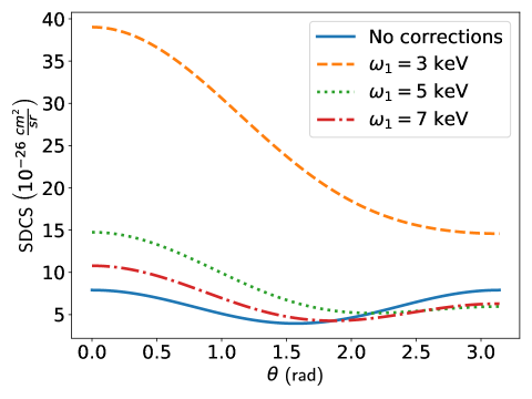
Figure 2: (Color online) SDCS in the case of hydrogen atom eq. (31) for three photon energies: 3 keV (dashed orange line), 5 keV (dotted green line) and 7 keV (dash-dotted red line). Blue solid line is the Thomson limit.

We see that the single differential cross section for the hydrogen atom at 3 keV is essentially larger than the Thomson cross section and behaves rather differently from it. However, this cross section falls rapidly with the growth of the photon energy. The single differential cross section at 5 keV has a minimum, which approaches the minimum of the Thomson cross section as the photon energy goes to 7 keV. At the photon energy of about 25 keV the inaccuracy of formula (31) for the hydrogen atom becomes larger than its deviation from the Thomson cross section, and in the energy range above it the Klein-Nishina-Tamm formula for Compton scattering at free electron can be used to describe Compton scattering from hydrogen atoms with a high accuracy.

Compton scattering from helium atoms is described by formula (2.2) and is very similar to that of hydrogen. The best accuracy of this formula is expected to be achieved for the photon energy $\omega_{1}\simeq\sqrt{m|\epsilon_{s}|}\simeq 4.45$ keV and is also about 1%. The single differential cross section for the helium atom for the photon energies 6, 9 and 12 keV, together with the doubled Thomson differential cross section for the electron, is presented in Fig. 3.

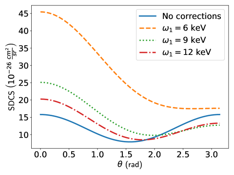
Figure 3: (Color online) SDCS in the case of helium atom eq. (2.2) for three photon energies: 6 keV (dashed orange line), 9 keV (dotted green line) and 12 keV (dash-dotted red line). Blue solid line is the Thomson limit.

Again we see that the single differential cross section at 6 keV is much larger than the Thomson cross section and has a rather different shape. We also see that, with the growth of the photon energy, the single differential cross section develops a minimum and becomes more similar to the Thomson cross section. At the photon energy of about 32 keV the inaccuracy of formula (2.2) for the helium atom becomes larger than its deviation from the doubled Thomson cross section, which means that in the energy range above it the Klein-Nishina-Tamm formula for Compton scattering at free electrons can be used to describe Compton scattering from helium atoms.

Next we pass to calculating the fully differential cross section of Compton scattering from hydrogen. To calculate this cross section it is convenient to introduce dimensionless variables in accordance with the following notations:

$$\gamma=a_{0}\omega_{1}=\frac{\omega_{1}}{me^{2}}=\frac{1}{\alpha}\left(\frac{\omega}{m}\right)=0.27\ \omega(keV),\quad\mu=a_{0}Q\approx\gamma\sqrt{2(1-\cos\theta)},$$

$$\quad x=a_{0}p=\frac{1}{\alpha}\sqrt{\frac{2E_{e}}{m}}\approx 0.27\sqrt{E_{e}(eV)},\quad e^{2}=\alpha=\frac{1}{137}.$$

Substituting Coulomb correction (2.1) into fully differential cross section (FDCS) (2.1) we get the following expression for the FDCS in terms of the dimensionless variables

$$\frac{d^{3}\sigma}{d\Omega_{\vec{k}_{2}}d\Omega_{e}dE_{e}}=\frac{32}{\pi}(\alpha a_{0})^{3}\mu^{2}\left(\frac{\exp\left[-\frac{2}{x}\arctan\frac{x}{\mu^{2}-x^{2}+1}\right]}{1-e^{-2\pi/x}}\right)$$

$$\times\left[\left(\frac{1+\mu^{2}+x^{2}-2\mu x\cos\chi}{2\gamma^{2}}+\cos\theta\right)^{2}+1\right]$$

$$\times\frac{(\mu-x\cos\chi)^{2}+\cos^{2}\chi}{[(\mu^{2}-x^{2}+1)^{2}+4x^{2}][\mu^{2}+x^{2}+1-2\mu x\cos\chi]^{4}}.$$ (41)

Next we observe that $(\alpha a_{0})^{3}=(1/m)^{2}(1/m)=1.491\cdot 10^{-21}(cm^{2})\times(1/5.11\cdot 10^{5}(eV))=0.29\cdot 10^{-26}(cm^{2}/eV)$. Thus, we obtain the cross section in $cm^{2}/sr^{2}\cdot eV$.

Integrating formula (3) with respect to $\chi$ gives us double differential cross section (DDCS), or the energy spectrum of electrons in the case, where the vectors $\vec{k}_{1},\vec{k}_{2},\vec{p}$   lie in the same plane (in the scattering plane)

$$\frac{d^{2}\sigma}{d\Omega_{\vec{k}_{2}}dE_{e}}=(2\pi)\int_{0}^{\pi}\ \frac{d^{3}\sigma}{d\Omega_{\vec{k}_{2}}d\Omega_{e}dE_{e}}\ \sin\chi\ d\chi.$$ (42)

The results of calculating the DDCS with the help of this formula are presented in Fig. 4 for the scattering angle $\theta=0.1$ rad and in Fig. 5 for the scattering angle $\theta=\pi/4$.

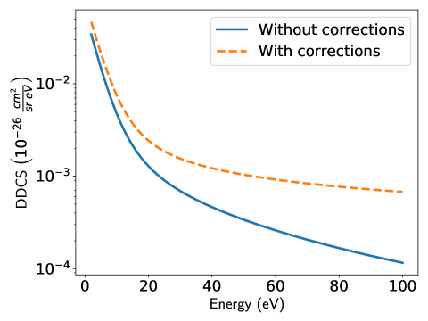
Figure 4: (Color online) DDCS eq. (42) versus the energy of the escaped electron in the case of hydrogen atom. The orange dashed curve corresponds to eq. (3) with the correction terms in the big square brackets. The solid blue line corresponds to eq. (3) without these terms. The photon energy $\omega_{1}=5$ keV, the scattering angle $\theta=0.1$ rad.

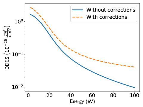
Figure 5: (Color online) The same as in Fig. 4 for the scattering angle $\theta=\pi/4$.

We see that the higher the electron energy is, the larger is the difference between the curves both in Fig. 4 and Fig. 5. However, in this energy range the DDCS is extremely small (we note that the DDCS is presented in the logarithmic scale).

For small electron energies the difference between the curves is not so noticeable. Besides, we see that larger momentum transfers $Q$ (big angles $\theta<\pi/2$) increase the absolute value of DDCS. Thus, we can conclude that, at relatively large momentum transfers, Compton scattering from hydrogen is accessible for experimental studies. Figs. 2 and 3 suggest that the DDCS of Compton scattering from helium atoms should be even larger. A detailed study of this case will be carried out in a separate paper.

4 Conclusions

In the present paper we have put forward a new approach to describing Compton scattering by bound electrons and applied it to the hydrogen and helium atoms. The approach is based on a relativistic version of the AA-approximation in the standard perturbative S-matrix formalism and allows one to describe this process consistently in the range of the photon energy $\omega_{1}$ satisfying the conditions $|\varepsilon|/\omega_{1}\ll 1$ and $\omega_{1}/m\ll 1$. For the hydrogen and helium atoms this is the energy range of several keV.

The obtained formulas for the cross section take into account the effects of boundness and correctly reproduce the high photon energy behavior, which is just the Klein-Nishina-Tamm cross section.

In the present paper we have considered only the case of unpolarized photons. However, the results can be easily generalized to the case of polarized incoming and outgoing photons. In the case of helium, the formulas can also be improved by taking realistic wave functions for the helium ground state. However, this will result in much more complicated calculations and will be discussed separately.

5 Acknowledgements

The authors thank Prof. R. Dörner and Dr. M. Schöffler for presenting some materials, which motivated us to carry out this investigation. We also thank Prof. O. Chuluunbaatar for some help in numerical calculations. Y.P. is grateful to the Russian Foundation for Basic Research (RFBR) for financial support under Grant 16-02-00049-a.

References

- [1] O. Klein and Y. Nishina “Über die Streuung von Strahlung durch freie Elektronen nach der neuen relativistischen Quantendynamik von Dirac” In Zeitschrift für Physik 52.11-12 Springer, 1929, pp. 853–868
- [2] I. Tamm “Über die Wechselwirkung der freien Elektronen mit der Strahlung nach der Diracsehen Theorie des Elektrons und nach der Quantenelektrodynamik” In Zeitschrift für Physik 62.7-8 Springer, 1930, pp. 545–568
- [3] V.. Berestetskii, L.. Landau, E.. Lifshitz and L.. Pitaevskii “Quantum electrodynamics” Butterworth-Heinemann, 1982
- [4] A.. Akhiezer and V.. Berestetskii “Quantum electrodynamics” John Wiley & Sons, 1965
- [5] A.. Dykhne and G.. Yudin “Sudden perturbations and quantum evolution” In Uspekhi Fiz. Nauk, 1996
- [6] Z. Kaliman, T. Surić, K. Pisk and R.. Pratt “Triply differential cross section for Compton scattering” In Physical Review A 57.4 APS, 1998, pp. 2683
- [7] R.. Pratt, L.. LaJohn, V. Florescu, T. Surić, B.. Chatterjee and S.. Roy “Compton scattering revisited” In Radiation Physics and Chemistry 79.2 Elsevier, 2010, pp. 124–131
- [8] K. Pisk, Z. Kaliman and N. Erceg “Wave–particle duality of radiation in Compton scattering” In Journal of Physics B: Atomic, Molecular and Optical Physics 49.23 IOP Publishing, 2016, pp. 235004
- [9] V.. Neudachin, Y.. Popov and Y.. Smirnov “Electron momentum spectroscopy of atoms, molecules, and thin films” In Physics-Uspekhi 42.10 Turpion Ltd, 1999, pp. 1017–1044
- [10] E. Weigold and I. McCarthy “Electron momentum spectroscopy” Kluwer, New York, 1999
- [11] F. Bell, A.. Rollason, J.. Schneider and W. Drube “Determination of electron momentum densities by a (, e) experiment” In Physical Review B 41.8 APS, 1990, pp. 4887
- [12] F. Bell, Th. Tschentscher, J.. Schneider and A.. Rollason “The triple differential cross section for deep inelastic photon scattering: a (gamma, e gamma’) experiment” In Journal of Physics B: Atomic, Molecular and Optical Physics 24.22 IOP Publishing, 1991, pp. L533