Abstract

Given $0<\alpha<1$, the Beatty sequence of density $\alpha$ is the sequence $B_{\alpha}=(\lfloor n/\alpha\rfloor)_{n\in\mathbb{N}}$. Beatty’s theorem states that if $\alpha,\beta$ are irrational numbers with $\alpha+\beta=1$, then the Beatty sequences $B_{\alpha}$ and $B_{\beta}$ partition the positive integers; that is, each positive integer belongs to exactly one of these two sequences. On the other hand, Uspensky showed that this result breaks down completely for partitions into three (or more) sequences: There does not exist a single triple $(\alpha,\beta,\gamma)$ such that the Beatty sequences $B_{\alpha},B_{\beta},B_{\gamma}$ partition the positive integers.

In this paper we consider the question of how close we can come to a three-part Beatty partition by considering “almost” Beatty sequences, that is, sequences that represent small perturbations of an “exact” Beatty sequence. We first characterize all cases in which there exists a partition into two exact Beatty sequences and one almost Beatty sequence with given densities, and we determine the approximation error involved. We then give two general constructions that yield partitions into one exact Beatty sequence and two almost Beatty sequences with prescribed densities, and we determine the approximation error in these constructions. Finally, we show that in many situations these constructions are best-possible in the sense that they yield the closest approximation to a three-part Beatty partition.

1 Introduction

A Beatty sequence is a sequence of the form $B_{\alpha}=({\lfloor n/\alpha\rfloor})_{n\in\mathbb{N}}$, where $0<\alpha<1$ is a real number and the bracket notation denotes the floor (or greatest integer) function. Beatty sequences arise in a variety of areas, from diophantine approximation and dynamical systems to theoretical computer science and the theory of quasicrystals. They have a number of remarkable properties, the most famous of which is the following theorem. Here, and in the sequel, $\mathbb{N}=\{1,2,3,\dots\}$ denotes the set of positive integers, and by a partition of $\mathbb{N}$ we mean a collection of subsets of $\mathbb{N}$ such that every element of $\mathbb{N}$ belongs to exactly one of these subsets.

Theorem A (Beatty’s theorem, [4]).

Two Beatty sequences $B_{\alpha}$ and $B_{\beta}$ partition $\mathbb{N}$ if and only if $\alpha$ and $\beta$ are positive irrational numbers with $\alpha+\beta=1$.

This result was posed in 1926 by Samuel Beatty as a problem in the American Mathematical Monthly [4], though it had appeared some 30 years earlier in a book by Rayleigh on the theory of sound [22, p. 123]. The result has been rediscovered multiple times since (e.g., [3, 24]), and it also appeared as a problem in the 1959 Putnam Competition [5]. The theorem has been variably referred to as Beatty’s theorem [13], Rayleigh’s theorem [23], and the Rayleigh-Beatty theorem [20]. For more about Beatty’s theorem, we refer to the paper by Stolarsky [26] and the references cited therein. Recent papers on the topic include Ginosar and Yona [11] and Kimberling and Stolarsky [16].

A notable feature of Beatty’s theorem is its generality: the only assumptions needed to ensure that two Beatty sequences form a partition of $\mathbb{N}$ are (1) the obvious requirement that the two densities add up to $1$, and (2) the (slightly less obvious, but not hard to verify) condition that the numbers $\alpha$ and $\beta$ be irrational.

As effective as Beatty’s theorem is in producing partitions of $\mathbb{N}$ into two Beatty sequences, the result breaks down completely for partitions into three (or more) such sequences:

Theorem B (Uspensky’s theorem, [29]).

There exists no partition of $\mathbb{N}$ into three or more Beatty sequences.

This result was first proved in 1927 by Uspensky [29]. Other proofs have been given by Skolem [24] and Graham [12]. As with Beatty’s theorem, Uspensky’s theorem eventually made its way into the Putnam, appearing as Problem B6 in the 1995 William Lowell Putnam Competition.

The theorems of Beatty and Uspensky can be stated in the following equivalent fashion, which highlights the complete breakdown of the partition property when more than two Beatty sequences are involved:

Theorem A^∗ (Complement version of Beatty’s theorem).

The complement of a Beatty sequence with irrational density is always another Beatty sequence.

Theorem B^∗ (Complement version of Uspensky’s theorem).

The complement of a union of two or more pairwise disjoint Beatty sequences is never a Beatty sequence.

In light of the results of Beatty and Uspensky on the existence (resp., non-existence) of partitions into two (resp., three) Beatty sequences it is natural to ask how close we can come to a partition of $\mathbb{N}$ into three Beatty sequences. Specifically, given irrational densities $\alpha,\beta,\gamma\in(0,1)$ that sum to $1$, can we obtain a proper partition of $\mathbb{N}$ by slightly “perturbing” one or more of the Beatty sequences $B_{\alpha},B_{\beta},B_{\gamma}$? If so, how many of the sequences $B_{\alpha},B_{\beta},B_{\gamma}$ do we need to perturb and what is the minimal amount of perturbation needed?

In this paper we seek to answer such questions by constructing partitions into “almost” Beatty sequences that approximate, in an appropriate sense, “exact” Beatty sequences. We call such partitions “almost Beatty partitions.”

Since, by Uspensky’s theorem, partitions into three Beatty sequences do not exist, the best we can hope for is partitions into two exact Beatty sequences, $B_{\alpha}$ and $B_{\beta}$, and an almost Beatty sequence $\widetilde{B_{\gamma}}$. In Theorem 1 we characterize all triples $(\alpha,\beta,\gamma)$ of irrational numbers for which such a partition exists, and we determine the precise “distance” (in the sense of (2) below) between the almost Beatty sequence $\widetilde{B_{\gamma}}$ and the corresponding exact Beatty sequence $B_{\gamma}$ in such a partition.

In Theorems 3, 4, and 6 we consider partitions into one exact Beatty sequence, $B_{\alpha}$, and two almost Beatty sequences, $\widetilde{B_{\beta}}$ and $\widetilde{B_{\gamma}}$, with given densities $\alpha$, $\beta$, and $\gamma$. In Theorem 3 we give a general construction of such partitions based on iterating the two-part Beatty partition process, and we determine the approximation errors involved. In Theorem 4 we present a different construction that requires a condition on the relative size of the densities $\alpha,\beta,\gamma$, but leads to a better approximation. In Theorem 6 we consider the special case when two of the three densities $\alpha,\beta,\gamma$ are equal, say $\alpha=\beta$. We show that in this case we can always obtain an almost Beatty partition from the Beatty sequences $B_{\alpha}$, $B_{\beta}(=B_{\alpha})$, and $B_{\gamma}$, by shifting all elements of $B_{\beta}$ and selected elements of $B_{\gamma}$ down by exactly $1$.

As special cases of the above results we recover, or improve on, some particular three-part almost Beatty partitions of $\mathbb{N}$ that have been mentioned in the literature; see Examples 2, 5, and 7. We emphasize that, while these particular partitions involve sequences with densities related to the golden ratio or other “special” irrational numbers, our results show that almost Beatty partitions of similar quality exist for any triple of irrational densities that sum up to $1$, with the quality of the approximation tied mainly to the size of these densities, and not their arithmetic nature.

Our final result, Theorem 8, is a non-existence result showing that the almost Beatty partitions obtained through the construction of Theorem 4 represent, in many situations, the closest approximation to a partition into three Beatty sequences that can be obtained by any method. Specifically, Theorem 8 shows that, for “generic” densities $\alpha,\beta,\gamma$ with $\alpha>1/3$, there does not exist an almost Beatty partition $\mathbb{N}=B_{\alpha}\cup\widetilde{B_{\beta}}\cup\widetilde{B_{\gamma}}$ in which the elements of the almost Beatty sequences $\widetilde{B_{\beta}}$ and $\widetilde{B_{\gamma}}$ differ from the corresponding elements of the exact Beatty sequences $B_{\beta}$ and $B_{\gamma}$ by at most $1$.

The remainder of this paper is organized as follows: In Section 2 we state our main results, Theorems 1–8, along with some examples illustrating these results. In Section 3 we gather some auxiliary results, while Sections 4–8 contain the proofs of our main results. We conclude in Section 9 with some remarks on related questions, extensions and generalizations of our results, and directions for future research.

2 Statement of Results

2.1 Notation and conventions

Given a real number $x$, we let ${\lfloor x\rfloor}$ denote its floor, defined as the largest integer $n$ such that $n\leq x$, and $\{x\}=x-{\lfloor x\rfloor}$ its fractional part.

We let $\mathbb{N}$ denote the set of positive integers, and we use capital letters $A,B,\dots$, to denote subsets of $\mathbb{N}$ or, equivalently, strictly increasing sequences of positive integers. We denote the $n$th elements of such sequences by $a(n)$, $b(n)$, etc.

It will be convenient to extend the definition of a sequence $(a(n))_{n\in\mathbb{N}}$ indexed by the natural numbers to a sequence indexed by the nonnegative integers by setting $a(0)=0$. For example, this convention allows us to consider the “gaps” $a(n)-a(n-1)$ for all $n\in\mathbb{N}$, with the initial gap, $a(1)-a(0)$, having the natural interpretation as the first element of the sequence.

Given a set $A\subset\mathbb{N}$, we denote by

$$A(n)=\#\{m\leq n:m\in A\}$$ (1)

the counting function of $A$, i.e., the number of elements of $A$ that are $\leq n$.

We measure the “closeness” of two sequences $(a(n))_{n\in\mathbb{N}}$ and $(b(n))_{n\in\mathbb{N}}$ by the sup-norm

$$\|a-b\| =\sup\{|a(n)-b(n)|:n\in\mathbb{N}\}.$$ (2)

Thus, $\|a-b\|<\infty$ holds if and only if one sequence can be obtained from the other by “perturbing” each element by a bounded quantity. For integers sequences the norm $\|a-b\|$ is attained and represents the maximal amount by which one sequence needs to be perturbed in order to obtain the other sequence.

2.2 Beatty sequences and almost Beatty sequences

Given $\alpha\in(0,1)$, we define the Beatty sequence of density $\alpha$ as

$$B_{\alpha} =(a(n))_{n\in\mathbb{N}},\quad a(n)={\lfloor n/\alpha\rfloor}.$$ (3)

We call a sequence $\widetilde{B_{\alpha}}=(\widetilde{a}(n))_{n\in\mathbb{N}}$ an almost Beatty sequence of density $\alpha$ if it satisfies $\|\widetilde{a}-a\|<\infty$, where $a(n)={\lfloor n/\alpha\rfloor}$ is the $n$th term of the Beatty sequence $B_{\alpha}$. Thus, an almost Beatty sequence is a sequence that can be obtained by perturbing the elements of a Beatty sequence by a bounded amount. Equivalently, an almost Beatty sequence of density $\alpha$ is a sequence $\widetilde{B_{\alpha}}$ satisfying

$$\widetilde{B_{\alpha}}(N)=\#\{n\leq N:n\in\widetilde{B_{\alpha}}\}=\alpha N+O(1)\quad(N\to\infty).$$

We use the analogous notation

$$B_{\beta} =({\lfloor n/\beta\rfloor})_{n\in\mathbb{N}}=(b(n))_{n\in\mathbb{N}},\quad\widetilde{B_{\beta}}=(\widetilde{b}(n))_{n\in\mathbb{N}},$$ (4)

$$B_{\gamma} =({\lfloor n/\gamma\rfloor})_{n\in\mathbb{N}}=(c(n))_{n\in\mathbb{N}},\quad\widetilde{B_{\gamma}}=(\widetilde{c}(n))_{n\in\mathbb{N}},$$ (5)

to denote Beatty sequences and almost Beatty sequences of densities $\beta$ and $\gamma$.

In the sequel, the notations $a(n)$, $b(n)$, and $c(n)$ will always refer to the elements of the Beatty sequences $B_{\alpha},B_{\beta},B_{\gamma}$ as defined in (3), (4), and (5), and $\widetilde{a}(n)$, $\widetilde{b}(n)$, and $\widetilde{c}(n)$ will refer to the elements of almost Beatty sequences $\widetilde{B_{\alpha}}$, $\widetilde{B_{\beta}}$, and $\widetilde{B_{\gamma}}$, of densities $\alpha$, $\beta$, and $\gamma$, respectively.

2.3 Partitions into two exact Beatty sequences and one almost Beatty sequence

We assume that we are given arbitrary positive real numbers $\alpha$, $\beta$, and $\gamma$ subject only to the conditions

$$\alpha,\beta,\gamma\in\mathbb{R}^{+}\setminus\mathbb{Q},\quad\alpha+\beta+\gamma=1,$$ (6)

which are analogous to the conditions in Beatty’s theorem (Theorem A). Our goal is to construct a partition of $\mathbb{N}$ into almost Beatty sequences $\widetilde{B_{\alpha}},\widetilde{B_{\beta}},\widetilde{B_{\gamma}}$ that are as close as possible to the exact Beatty sequences $B_{\alpha},B_{\beta},B_{\gamma}$, where “closeness” is measured by the distance (2).

By Uspensky’s theorem (Theorem B), a partition of $\mathbb{N}$ into three exact Beatty sequences is impossible, so the best we can hope for is a partition into two exact Beatty sequences $B_{\alpha}$ and $B_{\beta}$ and one almost Beatty sequence $\widetilde{B_{\gamma}}$. Our first theorem shows that such partitions do exist, it gives necessary and sufficient conditions on the densities $\alpha,\beta,\gamma$ under which such a partition exists, and it shows exactly how close the almost Beatty sequence $\widetilde{B_{\gamma}}$ is to the exact Beatty sequence $B_{\gamma}$.

Theorem 1 (Partition into two exact Beatty sequences and one almost Beatty sequence).

Let $\alpha,\beta,\gamma$ satisfy (6). Then there exists a partition $\mathbb{N}=\widetilde{B_{\alpha}}\cup\widetilde{B_{\beta}}\cup\widetilde{B_{\gamma}}$ with $\widetilde{B_{\alpha}}=B_{\alpha}$, $\widetilde{B_{\beta}}=B_{\beta}$ if and only if

$$r\alpha+s\beta=1\quad\text{for some $r,s\in\mathbb{N}$.}$$ (7)

If this condition is satisfied, then $B_{\alpha}$ and $B_{\beta}$ are disjoint and $\widetilde{B_{\gamma}}=\mathbb{N}\setminus(B_{\alpha}\cup B_{\beta})$ is an almost Beatty sequence satisfying

$$\|\widetilde{c}-c\| =\max\left(\left\lfloor\frac{2-\alpha}{1-\alpha}\right\rfloor,\left\lfloor\frac{2-\beta}{1-\beta}\right\rfloor\right),$$ (8)

where $c(n)={\lfloor n/\gamma\rfloor}$, resp., $\widetilde{c}(n)$, denote the $n$th elements of $B_{\gamma}$, resp., $\widetilde{B_{\gamma}}$. More precisely, we have

$$0\leq c(n)-\widetilde{c}(n)\leq\max\left(\left\lfloor\frac{2-\alpha}{1-\alpha}\right\rfloor,\left\lfloor\frac{2-\beta}{1-\beta}\right\rfloor\right)\quad(n\in\mathbb{N}),$$ (9)

where the upper bound is attained for infinitely many $n$. In particular, if $\alpha$ and $\beta$ satisfy

$$\max(\alpha,\beta)<1/2,$$ (10)

then we have

$$c(n)-\widetilde{c}(n)\in\{0,1,2\}\quad(n\in\mathbb{N}).$$ (11)

The error bound (9) in this theorem is best-possible in the strongest possible sense: There does not exist a single triple $(\alpha,\beta,\gamma)$ of irrational densities satisfying the assumptions of Theorem 1 for which this bound can be improved. In particular, since

$$\left\lfloor\frac{2-t}{1-t}\right\rfloor=\left\lfloor 1+\frac{1}{1-t}\right\rfloor\geq 2\quad(0<t<1),$$

it follows that there exists no partition into two exact Beatty sequences and an almost Beatty sequence whose elements differ from the elements of the corresponding exact Beatty sequence by at most $1$. Put differently, if only one of the three Beatty sequences is perturbed, the minimal amount of perturbation (in the sense of the distance (2)) needed in order to obtain a partition of $\mathbb{N}$ is $2$. Moreover, by Theorem 1 a perturbation by at most $2$ is sufficient if and only if the conditions (6) and (7) are satisfied and $\max(\alpha,\beta)<1/2$.

Example 2.

Let $\alpha=1/\Phi^{3}$, $\beta=1/\Phi^{4}$, $\gamma=1/\Phi$, where $\Phi=(\sqrt{5}+1)/2=1.61803\dots$ is the golden ratio. Using the relation $\Phi^{2}=\Phi+1$ one can check that $1/\Phi^{3}+1/\Phi^{4}+1/\Phi=1$ and $3/\Phi^{3}+2/\Phi^{4}=1$, so conditions (6) and (7) of Theorem 1 hold. Moreover, since $\max(\alpha,\beta)<1/2$, by the last part of the theorem the perturbation errors $c(n)-\widetilde{c}(n)$ are in $\{0,1,2\}$. Table 1 shows the partition $\mathbb{N}=B_{\alpha}\cup B_{\beta}\cup\widetilde{B_{\gamma}}$ obtained from the theorem, along with the perturbation errors. The two exact Beatty sequences $B_{\alpha}$ and $B_{\beta}$ in this partition are the sequences A004976 and A004919 in OEIS [25], while the almost Beatty sequence $\widetilde{B_{\gamma}}$ is a perturbation of the sequence A000201, obtained by subtracting an appropriate amount in $\{0,1,2\}$ from the elements in A000201.

$a(n)$	4	8	12	16	21	25	29	33	38	42	46	50	55	59	63
$b(n)$	6	13	20	27	34	41	47	54	61	68	75	82	89	95	102
$c(n)$	1	3	4	6	8	9	11	12	14	16	17	19	21	22	24
$\widetilde{c}(n)$	1	2	3	5	7	9	10	11	14	15	17	18	19	22	23
Error	0	1	1	1	1	0	1	1	0	1	0	1	2	0	1

Table 1: An almost Beatty partition with $\alpha=1/\Phi^{3}$, $\beta=1/\Phi^{4}$, $\gamma=1/\Phi$. (The three highlighted rows form the partition.)

2.4 Partitions into one exact Beatty sequence and two almost Beatty sequences

We next consider partitions into one exact Beatty sequence and two almost Beatty sequences. In contrast to the situation in Theorem 1, here the two almost Beatty sequences are not uniquely determined. We give two constructions that lead to different partitions. Our first approach is based on iterating the two-part Beatty partition process and leads to the following result.

Theorem 3 (Partition into one exact Beatty sequence and two almost Beatty sequences—Construction I).

Let $\alpha,\beta,\gamma$ satisfy (6) and suppose

$$\frac{\beta}{\gamma}\not\in\mathbb{Q}.$$ (12)

Let

$$\widetilde{b}(n)={\left\lfloor{\left\lfloor\frac{1-\alpha}{\beta}n\right\rfloor}\frac{1}{1-\alpha}\right\rfloor},\quad\widetilde{c}(n)={\left\lfloor{\left\lfloor\frac{1-\alpha}{\gamma}n\right\rfloor}\frac{1}{1-\alpha}\right\rfloor}.$$ (13)

Then the sequences $B_{\alpha}$, $\widetilde{B_{\beta}}=(\widetilde{b}(n))_{n\in\mathbb{N}}$, and $\widetilde{B_{\gamma}}=(\widetilde{c}(n))_{n\in\mathbb{N}}$ form an almost Beatty partition of $\mathbb{N}$ satisfying

$$\|\widetilde{b}-b\| \leq\left\lfloor\frac{2-\alpha}{1-\alpha}\right\rfloor,\quad\|\widetilde{c}-c\|\leq\left\lfloor\frac{2-\alpha}{1-\alpha}\right\rfloor.$$ (14)

In particular, if $\alpha$ satisfies

$$\alpha<1/2,$$ (15)

then we have

$$\|\widetilde{b}-b\|\leq 2,\quad\|\widetilde{c}-c\|\leq 2.$$ (16)

Our second construction consists of starting out with two exact Beatty sequences $B_{\alpha}$ and $B_{\beta}$, and then shifting those elements of $B_{\beta}$ that also belong to $B_{\alpha}$ to get a sequence $\widetilde{B_{\beta}}$ that is disjoint from $B_{\alpha}$.

Theorem 4 (Partition into one exact Beatty sequence and two almost Beatty sequences—Construction II).

Let $\alpha,\beta,\gamma$ satisfy (6) and suppose

$$\max(\alpha,\beta)<\gamma.$$ (17)

Let $\widetilde{B_{\beta}}=(\widetilde{b}(n))_{n\in\mathbb{N}}$ be defined by

$$\widetilde{b}(n)=\begin{cases}b(n),&\text{if $b(n)\not\in B_{\alpha}$;}\\ b(n)-1,&\text{if $b(n)\in B_{\alpha}$,}\end{cases}$$ (18)

and let $\widetilde{B_{\gamma}}=\mathbb{N}\setminus(B_{\alpha}\cup\widetilde{B_{\beta}})=(\widetilde{c}(n))_{n\in\mathbb{N}}$. Then the sequences $B_{\alpha}$, $\widetilde{B_{\beta}}$, and $\widetilde{B_{\gamma}}$ form an almost Beatty partition of $\mathbb{N}$ satisfying

$$\|\widetilde{b}-b\| \leq 1,\quad\|\widetilde{c}-c\|\leq 2.$$ (19)

More precisely, we have

$$b(n)-\widetilde{b}(n) \in\{0,1\}\quad(n\in\mathbb{N}),$$ (20)

$$c(n)-\widetilde{c}(n) \in\{0,1,2\}\quad(n\in\mathbb{N}).$$ (21)

Our proof will yield a more precise result that gives necessary and sufficient conditions for each of the three possible values in (21), and which allows one, in principle, to determine the relative frequencies of these values.

Example 5.

Let $\tau=1.83929\dots$ be the Tribonacci constant, defined as the positive root of $1/\tau+1/\tau^{2}+1/\tau^{3}=1$, and let $\alpha=1/\tau^{3}$, $\beta=1/\tau^{2}$, $\gamma=1/\tau$. Then $\alpha,\beta,\gamma$ satisfy the conditions (6) and (17) of Theorem 4. Thus, Theorem 4 can be applied to yield a partition of $\mathbb{N}$ into the exact Beatty sequence $B_{\alpha}=B_{1/\tau^{3}}$ and two almost Beatty sequences $\widetilde{B_{\beta}}$ and $\widetilde{B_{\gamma}}$ of densities $1/\tau^{2}$ and $1/\tau$, respectively, with perturbation errors in $\{0,1\}$ for the former sequence, and in $\{0,1,2\}$ for the latter sequence. The resulting partition is shown in Table 2 below.

The sequences $B_{\alpha},B_{\beta},B_{\gamma}$ are the OEIS sequences A277723, A277722, A158919, respectively, while sequence A277728 represents the numbers not in any of these sequences. The OEIS entry for the latter sequence mentions three related sequences, A003144, A003145, and A003146, that do form a partition of $\mathbb{N}$ and which differ from $B_{\alpha}$, $B_{\beta}$, and $B_{\gamma}$ by at most $3$. The partition obtained by Theorem 4 is different from this partition, and it yields a better approximation to a proper Beatty partition, with perturbation errors of $2$ in the case of $\widetilde{B_{\gamma}}$, and $1$ in the case of $\widetilde{B_{\beta}}$.

$a(n)$	6	12	18	24	31	37	43	49	56	62	68	74	80	87	93
$b(n)$	3	6	10	13	16	20	23	27	30	33	37	40	43	47	50
$\widetilde{b}(n)$	3	5	10	13	16	20	23	27	30	33	36	40	42	47	50
Error	0	1	0	0	0	0	0	0	0	0	1	0	1	0	0
$c(n)$	1	4	6	7	10	13	13	14	17	19	21	23	24	25	28
$\widetilde{c}(n)$	1	3	5	7	9	11	12	14	16	18	20	22	23	25	27
Error	0	1	1	0	1	2	1	0	1	1	1	1	1	0	1

Table 2: An almost Beatty partition with $\alpha=1/\tau^{3}$, $\beta=1/\tau^{2}$, $\gamma=1/\tau$.

It is interesting to compare the constructions of Theorem 3 and Theorem 4. Both constructions are applicable under slightly different additional conditions beyond (6): Theorem 3 requires that $\beta/\gamma$ be irrational, while Theorem 4 requires that $\gamma>\max(\alpha,\beta)$. Thus, the results are not directly comparable. However, in cases where both constructions can be applied, the construction of Theorem 4 yields stronger bounds than those that can be obtained from Theorem 3, namely $\|\widetilde{b}-b\|\leq 1$ and $\|\widetilde{c}-c\|\leq 2$ instead of $\|\widetilde{b}-b\|\leq 2$ and $\|\widetilde{c}-c\|\leq 2$.

2.5 Partitions into one exact Beatty sequence and two almost Beatty sequences: The case of two equal densities

In the case when the densities $\alpha$ and $\beta$ are equal, we can improve on the bounds (19) of Theorem 4.

Theorem 6 (Partition into one exact Beatty sequence and two almost Beatty sequences—Special case).

Let $\alpha,\beta,\gamma$ satisfy (6), and suppose $\beta=\alpha$. Let $\widetilde{B_{\beta}}=(\widetilde{b}(n))_{n\in\mathbb{N}}$ be defined by

$$\widetilde{b}(n)=b(n)-1\quad(n\in\mathbb{N}),$$ (22)

and let $\widetilde{B_{\gamma}}=\mathbb{N}\setminus(B_{\alpha}\cup\widetilde{B_{\beta}})=(\widetilde{c}(n))_{n\in\mathbb{N}}$. Then the sequences $B_{\alpha}$, $\widetilde{B_{\beta}}$, and $\widetilde{B_{\gamma}}$ form an almost Beatty partition of $\mathbb{N}$ satisfying

$$\|\widetilde{b}-b\|=1,\quad\|\widetilde{c}-c\|\leq 1.$$ (23)

More precisely, we have

$$b(n)-\widetilde{b}(n) =1\quad(n\in\mathbb{N}),$$ (24)

$$c(n)-\widetilde{c}(n) \in\{0,1\}\quad(n\in\mathbb{N}).$$ (25)

Example 7.

Let $\alpha=\beta=1/\Phi^{2}$ and $\gamma=1/\Phi^{3}$, where $\Phi$ is the golden ratio. Since $1/\Phi^{3}=1/\Phi-1/\Phi^{2}$, we have $\alpha+\beta+\gamma=1/\Phi^{2}+1/\Phi=1$, so the density condition (6) is satisfied and Theorem 6 yields an almost Beatty partition consisting of the sequences $B_{\alpha}=({\lfloor\Phi^{2}n\rfloor})_{n\in\mathbb{N}}$, $B_{\beta}=B_{\alpha}-1=({\lfloor\Phi^{2}n\rfloor}-1)_{n\in\mathbb{N}}$, and $\widetilde{B_{\gamma}}$, where the elements of $\widetilde{B_{\gamma}}$ differ from those of $B_{\gamma}=({\lfloor\Phi^{3}n\rfloor})_{n\in\mathbb{N}}$ by at most $1$. In fact, the elementary identity ${\lfloor\Phi^{2}n\rfloor}-1={\lfloor\Phi{\lfloor\Phi n\rfloor}\rfloor}$ shows that this partition is the same as that obtained by Theorem 3, namely

$$\mathbb{N}=({\lfloor\Phi^{2}n\rfloor})_{n\in\mathbb{N}}\cup({\lfloor\Phi{\lfloor\Phi n\rfloor}\rfloor})_{n\in\mathbb{N}}\cup({\lfloor\Phi{\lfloor\Phi^{2}n\rfloor}\rfloor})_{n\in\mathbb{N}}.$$

This particular partition is known. It was mentioned in Skolem [24, p. 68], and it can be interpreted in terms of Wythoff sequences; see the OEIS sequence A003623.

We remark that, while the identity ${\lfloor\Phi^{2}n\rfloor}-1={\lfloor\Phi{\lfloor\Phi n\rfloor}\rfloor}$, and hence the connection with the iterated Beatty partition construction, is closely tied to properties of the golden ratio, Theorem 6 shows that almost Beatty partitions of the same quality (i.e., with one exact Beatty sequence and two almost Beatty sequences with perturbation errors at most $1$) exist whenever two of the densities $\alpha,\beta,\gamma$ are equal.

The constructions of both Theorem 6 and Theorem 1 can be viewed as special cases of the construction of Theorem 4. Indeed, if $B_{\alpha}=B_{\beta}$, then the formula for $\widetilde{b}(n)$ of Theorem 4 reduces to $\widetilde{b}(n)=b(n)-1$ for all $n$, while in the case when $B_{\alpha}$ and $B_{\beta}$ are disjoint, this formula yields $\widetilde{b}(n)=b(n)$ for all $n$ and thus $\widetilde{B_{\beta}}=B_{\beta}$. We note, however, that Theorems 1 and 6 are more general in one respect: they do not require the condition (17) of Theorem 4.

2.6 A non-existence result

As mentioned in the remarks following Theorem 1, the bounds on the perturbation errors in this result are best-possible. As a consequence, there exists no partition $\mathbb{N}=\widetilde{B_{\alpha}}\cup\widetilde{B_{\beta}}\cup\widetilde{B_{\gamma}}$ such that $\widetilde{B_{\alpha}}=B_{\alpha}$ and $\widetilde{B_{\beta}}=B_{\beta}$ are exact Beatty sequences and $\widetilde{B_{\gamma}}$ is an almost Beatty sequence satisfying $\|\widetilde{c}-c\|\leq 1$.

A similarly universal optimality result does not hold for the bound $\|c-\widetilde{c}\|\leq 2$ in Theorem 4. Indeed, as Theorem 6 shows, in the case of two equal densities this bound can be improved to $\|c-\widetilde{c}\|\leq 1$. In the following theorem we show that, for “generic” densities $\alpha,\beta,\gamma$ with $\alpha>1/3$, the error bound $\|c-\widetilde{c}\|\leq 2$ is indeed best-possible.

Theorem 8 (Non-existence of partitions into an exact Beatty sequence and two almost Beatty sequences with perturbation errors $\leq 1$).

Let $\alpha,\beta,\gamma$ satisfy (6) and suppose that

$$\alpha>1/3,$$ (26)

$$1,\alpha,\beta \mathbb{Q}$$ are linearly independent over . (27)

There exists no partition $\mathbb{N}=\widetilde{B_{\alpha}}\cup\widetilde{B_{\beta}}\cup\widetilde{B_{\gamma}}$ such that $\widetilde{B_{\alpha}}=B_{\alpha}$ is an exact Beatty sequence and $\widetilde{B_{\beta}}=(\widetilde{b}(n))_{n\in\mathbb{N}}$ and $\widetilde{B_{\gamma}}=(\widetilde{c}(n))_{n\in\mathbb{N}}$ are almost Beatty sequences of densities $\beta$ and $\gamma$, respectively, satisfying $\|\widetilde{b}-b\|\leq 1$ and $\|\widetilde{c}-c\|\leq 1$.

3 Lemmas

We begin by stating, without proof, some elementary relations involving the floor and fractional part functions.

Lemma 9 (Floor and fractional part function identities).

For any real numbers $x,y$ we have

$${\lfloor x+y\rfloor} ={\lfloor x\rfloor}+{\lfloor y\rfloor}+\delta(\{x\},\{y\}),$$

$${\lfloor x-y\rfloor} ={\lfloor x\rfloor}-{\lfloor y\rfloor}-\delta(\{x-y\},\{y\}),$$

$$\{x+y\} =\{x\}+\{y\}-\delta(\{x\},\{y\}),$$

$$\{x-y\} =\{x\}-\{y\}+\delta(\{x-y\},\{y\}),$$

where

$$\delta(s,t)=\begin{cases}1,&\text{if $s+t\geq 1$;}\\ 0,&\text{if $s+t<1$.}\end{cases}$$ (28)

In the following lemma we collect some elementary properties of Beatty sequences. We will provide proofs for the sake of completeness.

Lemma 10 (Elementary properties of Beatty sequences).

Let $\alpha\in(0,1)$ be irrational, and let $B_{\alpha}=(a(n))_{n\in\mathbb{N}}=({\lfloor n/\alpha\rfloor})_{n\in\mathbb{N}}$ be the Beatty sequence of density $\alpha$.

• Membership criterion: For any $m\in\mathbb{N}$ we have

  $$m\in B_{\alpha}\Longleftrightarrow\{(m+1)\alpha\}<\alpha\Longleftrightarrow\{m\alpha\}>1-\alpha.$$

• Counting function formula: For any $m\in\mathbb{N}$ we have

  $$B_{\alpha}(m)={\lfloor\alpha(m+1)\rfloor}=\alpha m+\alpha-\{\alpha(m+1)\},$$

  where $B_{\alpha}(m)$ is the counting function of $B_{\alpha}$, as defined in (1).

• Gap formula: Let $k={\lfloor 1/\alpha\rfloor}$. For any $n\in\mathbb{N}$ we have

  $$a(n+1)-a(n)=\begin{cases}k+1,&\text{if $\{n/\alpha\}\geq 1-\{1/\alpha\}$;}\\ k,&\text{otherwise.}\end{cases}$$

• Gap criterion: Given $m\in B_{\alpha}$, let $m^{\prime}$ denote the successor to $m$ in the sequence $B_{\alpha}$, so that, by (iii), $m^{\prime}=m+k$ or $m^{\prime}=m+k+1$, where $k={\lfloor 1/\alpha\rfloor}$. Then we have, for any $m\in\mathbb{N}$,

  $$m\in B_{\alpha}\text{ and }m^{\prime}=m+k \Longleftrightarrow\{1/\alpha\}\alpha<\{(m+1)\alpha\}<\alpha,$$

  $$m\in B_{\alpha}\text{ and }m^{\prime}=m+k+1 \Longleftrightarrow\{(m+1)\alpha\}<\{1/\alpha\}\alpha.$$

Remark 11.

Our assumption that $\alpha$ is irrational ensures that equality cannot hold in any of the above relations.

Proof.

(i) We have

$$m\in B_{\alpha} \Longleftrightarrow m={\lfloor n/\alpha\rfloor}\text{ for some $n\in\mathbb{N}$}$$

$$\Longleftrightarrow m<n/\alpha<m+1\text{ for some $n\in\mathbb{N}$}$$

$$\Longleftrightarrow m\alpha<n<(m+1)\alpha\text{ for some $n\in\mathbb{N}$}$$

$$\Longleftrightarrow\{(m+1)\alpha\}<\alpha$$

$$\Longleftrightarrow\{m\alpha\}>1-\alpha.$$

(ii) We have

$$B_{\alpha}(m)=n \Longleftrightarrow{\lfloor n/\alpha\rfloor}\leq m\leq{\lfloor(n+1)/\alpha\rfloor}-1$$

$$\Longleftrightarrow n/\alpha<m+1<(n+1)/\alpha$$

$$\Longleftrightarrow n<(m+1)\alpha<n+1$$

$$\Longleftrightarrow n={\lfloor(m+1)\alpha\rfloor}=(m+1)\alpha-\{(m+1)\alpha\}.$$

(iii) By Lemma 9 we have

$$a(n+1)-a(n)={\left\lfloor\frac{n+1}{\alpha}\right\rfloor}-{\left\lfloor\frac{n}{\alpha}\right\rfloor}={\left\lfloor\frac{1}{\alpha}\right\rfloor}+\delta\left(\left\{\frac{1}{\alpha}\right\},\left\{\frac{n}{\alpha}\right\}\right),$$

where the last term is equal to $1$ if $\{1/\alpha\}+\{n/\alpha\}\geq 1$, and $0$ otherwise.

(iv) Note that

$$k\alpha=\left(\frac{1}{\alpha}-\left\{\frac{1}{\alpha}\right\}\right)\alpha=1-\left\{\frac{1}{\alpha}\right\}\alpha.$$

Thus, using the results of part (i) and (iii) we have

$$m\in B_{\alpha}\text{ and }m^{\prime}=m+k \Longleftrightarrow m\in B_{\alpha}\text{ and }m+k\in B_{\alpha}$$

$$\Longleftrightarrow\{(m+1)\alpha\}<\alpha\text{ and }\{(m+1)\alpha+k\alpha\}<\alpha$$

$$\Longleftrightarrow\{(m+1)\alpha\}<\alpha\text{ and }\{(m+1)\alpha-\{1/\alpha\}\alpha\}<\alpha$$

$$\Longleftrightarrow\{1/\alpha\}\alpha<\{(m+1)\alpha\}<\alpha.$$

This proves the first of the asserted equivalences in (iv). The second equivalence, asserting that $m\in B_{\alpha}$ and $m^{\prime}=m+k+1$ holds if and only if $\{(m+1)\alpha\}<\{1/\alpha\}\alpha$, follows from this on observing that, by (i), $m\in B_{\alpha}$ is equivalent to $\{(m+1)\alpha\}\in(0,\alpha)$, and by (iii) for any $m\in B_{\alpha}$, we have either $m^{\prime}=m+k$ or $m^{\prime}=m+k+1$. ∎

For our next lemma we assume that $\alpha,\beta,\gamma$ are irrational numbers satisfying (6), so that, in particular,

$$\gamma=1-\alpha-\beta,$$ (29)

and we define

$$u_{m}=\{(m+1)\alpha\},\quad v_{m}=\{(m+1)\beta\},\quad w_{m}=\{(m+1)\gamma\}.$$ (30)

Using (29), the latter quantity, $w_{m}$, can be expressed in terms of $u_{m}$ and $v_{m}$:

$$w_{m} =\{(m+1)(1-\alpha-\beta)\}=\{-(m+1)(\alpha+\beta)\}$$ (31)

$$=1-\{(m+1)\alpha+(m+1)\beta\}=1-\{u_{m}+v_{m}\}.$$

Lemma 12 (Counting function identity).

Let $\alpha,\beta,\gamma$ satisfy (6), and let $u_{m}$ and $v_{m}$ be as in (30). Then we have, for any $m\in\mathbb{N}$,

$$B_{\alpha}(m)+B_{\beta}(m)+B_{\gamma}(m)=m-\delta(u_{m},v_{m}),$$ (32)

where $\delta(s,t)\in\{0,1\}$ is given by (28).

Proof.

Using Lemma 10(ii) together with (29) and (31) we obtain

$$B_{\alpha}(m)+B_{\beta}(m)+B_{\gamma}(m) =(m+1)(\alpha+\beta+\gamma)-u_{m}-v_{m}-w_{m}$$

$$=m-u_{m}-v_{m}+\{u_{m}+v_{m}\}.$$

Since $u_{m},v_{m}\in(0,1)$, Lemma 9 yields $\{u_{m}+v_{m}\}=u_{m}+v_{m}-\delta(u_{m},v_{m})$. The desired identity now follows. ∎

The remaining lemmas in this section are deeper results which we quote from the literature. The first of these results characterizes disjoint Beatty sequences; see Theorem 3.11 in Niven [19].

Lemma 13 (Disjointness criterion).

Let $\alpha,\beta$ be irrational numbers in $(0,1)$. Then the Beatty sequences $B_{\alpha}$ and $B_{\beta}$ are disjoint if and only if there exist positive integers $r$ and $s$ such that

$$r\alpha+s\beta=1.$$ (33)

The next lemma is a special case of Weyl’s Theorem in the theory of uniform distribution modulo $1$; see Examples 2.1 and 6.1 in Chapter 1 of Kuipers and Niederreiter [18].

Lemma 14 (Weyl’s Theorem).

• Let $\theta$ be an irrational number. Then the sequence $(n\theta)_{n\in\mathbb{N}}$ is uniformly distributed modulo $1$; that is, we have

  $$\lim_{N\to\infty}\frac{1}{N}\#\{n\leq N:\{n\theta\}<t\}=t\quad(0\leq t\leq 1).$$

• Let $\theta_{1},\dots,\theta_{k}$ be real numbers such that the numbers $1,\theta_{1},\dots,\theta_{k}$ are linearly independent over $\mathbb{Q}$. Then the $k$-dimensional sequence $\{(n\theta_{1},\dots,n\theta_{k})\}$ is uniformly distributed modulo $1$ in $\mathbb{R}^{k}$; that is, we have

  $$\lim_{N\to\infty}\frac{1}{N}\#\{n\leq N:\{n\theta_{i}\}<t_{i}\text{ for $i=1,\dots,k$}\}=t_{1}\dots t_{k}\quad(0\leq t_{i}\leq 1).$$

4 Proof of Theorem 3

Let $\alpha,\beta,\gamma$ satisfy (6) and (12). Thus, $\alpha,\beta,\gamma$ are positive irrational numbers with $\alpha+\beta+\gamma=1$ and $\beta/\gamma$ irrational.

Since $\alpha$ is irrational, we can apply Beatty’s theorem (Theorem A) to the pair of densities $(\alpha,1-\alpha)$ to obtain a partition $\mathbb{N}=B_{\alpha}\cup B_{1-\alpha}$, where $B_{\alpha}$ is the exact Beatty sequence in the three-part partition we are trying to construct and

$$B_{1-\alpha}=\left({\left\lfloor n\frac{1}{1-\alpha}\right\rfloor}\right)_{n\in\mathbb{N}}.$$

We partition the latter sequence by partitioning the index set $\mathbb{N}$ into two Beatty sequences with densities $\beta/(1-\alpha)$ and $1-\beta/(1-\alpha)=\gamma/(1-\alpha)$. These densities sum to $1$, and our assumption that $\beta/\gamma$ is irrational ensures that both densities are irrational. Thus Beatty’s theorem can be applied again, yielding the partition

$$B_{1-\alpha}=\left({\left\lfloor{\left\lfloor\frac{1-\alpha}{\beta}n\right\rfloor}\frac{1}{1-\alpha}\right\rfloor}\right)_{n\in\mathbb{N}}\cup\left({\left\lfloor{\left\lfloor\frac{1-\alpha}{\gamma}n\right\rfloor}\frac{1}{1-\alpha}\right\rfloor}\right)_{n\in\mathbb{N}}.$$

The two sequences in this partition are exactly the sequences $\widetilde{B_{\beta}}=(\widetilde{b}(n))_{n\in\mathbb{N}}$ and $\widetilde{B_{\gamma}}=(\widetilde{c}(n))_{n\in\mathbb{N}}$ defined in Theorem 3. Thus, it remains to show that these sequences satisfy the bounds (14). By symmetry, it suffices to prove the first of these bounds, $\|\widetilde{b}-b\|\leq{\lfloor(2-\alpha)/(1-\alpha)\rfloor}$.

Using elementary properties of the floor and fractional part functions we have, for all $n\in\mathbb{N}$,

$$\widetilde{b}(n) ={\left\lfloor{\left\lfloor\frac{1-\alpha}{\beta}n\right\rfloor}\frac{1}{1-\alpha}\right\rfloor}\leq{\left\lfloor\frac{n}{\beta}\right\rfloor}=b(n)$$

and

$$\widetilde{b}(n) ={\left\lfloor\frac{n}{\beta}-\left\{\frac{1-\alpha}{\beta}n\right\}\frac{1}{1-\alpha}\right\rfloor}\geq{\left\lfloor\frac{n}{\beta}\right\rfloor}-{\left\lfloor\frac{1}{1-\alpha}\right\rfloor}-1$$

$$=b(n)-{\left\lfloor\frac{1}{1-\alpha}\right\rfloor}-1.$$

Hence

$$0\leq b(n)-\widetilde{b}(n)\leq{\left\lfloor\frac{1}{1-\alpha}\right\rfloor}+1={\left\lfloor\frac{2-\alpha}{1-\alpha}\right\rfloor}$$

for all $n\in\mathbb{N}$. It follows that $\|\widetilde{b}-b\|\leq{\lfloor(2-\alpha)/(1-\alpha)\rfloor}$, which is the asserted bound (14) for $\|\widetilde{b}-b\|$. This completes the proof of Theorem 3.

5 Proof of Theorem 4

Let $\alpha,\beta,\gamma$ satisfy the conditions (6) and (17) of Theorem 4. Thus, $\alpha,\beta,\gamma$ are positive irrational numbers satisfying $\alpha+\beta+\gamma=1$ and $\gamma>\max(\alpha,\beta)$. The latter two conditions imply

$$\alpha<1/2,\quad\beta<1/2,\quad\gamma>1/3.$$ (34)

Let $\widetilde{B_{\beta}}=\{\widetilde{b}(n)\}$ and $\widetilde{B_{\gamma}}=\mathbb{N}\setminus(B_{\alpha}\cup\widetilde{B_{\beta}})$ be the sequences defined in Theorem 4.

5.1 Proof of the partition property

We first show that the sequences $\widetilde{B_{\beta}}$ and $B_{\alpha}$ are disjoint. Consider an element $m=\widetilde{b}(n)\in\widetilde{B_{\beta}}$. By definition, we have $m=b(n)$ if $b(n)\not\in B_{\alpha}$, and $m=b(n)-1$ if $b(n)\in B_{\alpha}$. In the former case, we immediately get $m\not\in B_{\alpha}$, while in the latter case we have $m+1\in B_{\alpha}$, which by Lemma 10(iii) and the above assumption $\alpha<1/2$ implies $m\not\in B_{\alpha}$. Thus the sequences $B_{\alpha}$ and $\widetilde{B_{\beta}}$ are disjoint.

Since $\widetilde{B_{\gamma}}$ is defined as the complement of the sequences $B_{\alpha}$ and $\widetilde{B_{\beta}}$, it follows that the three sequences $B_{\alpha}$, $\widetilde{B_{\beta}}$, $\widetilde{B_{\gamma}}$ form a partition of $\mathbb{N}$, as claimed. ∎

5.2 Proof of the bounds (19) and (21)

The norm estimates (19) obviously follow from the definition of $\widetilde{b}(n)$ and (21), so it suffices to prove the latter relation, i.e.,

$$c(n)-\widetilde{c}(n)\in\{0,1,2\}\quad\text{for all $n\in\mathbb{N}$.}$$ (35)

We break up the argument into several lemmas. We recall the notation

$$u_{m} =\{(m+1)\alpha\},\quad v_{m}=\{(m+1)\beta\},\quad w_{m}=\{(m+1)\gamma\}=1-\{u_{m}+v_{m}\}.$$ (36)

We set

$$E_{\beta}(m)=\widetilde{B_{\beta}}(m)-B_{\beta}(m),\quad E_{\gamma}(m)=\widetilde{B_{\gamma}}(m)-B_{\gamma}(m).$$ (37)

Thus, the sequences $E_{\beta}$ and $E_{\gamma}$ represent the differences between the counting functions of the almost Beatty sequences $\widetilde{B_{\beta}}$ and $\widetilde{B_{\gamma}}$ and the counting functions of the corresponding exact Beatty sequences. In the following two lemmas we show that these differences are always in $\{0,1\}$, and we characterize the cases in which each of the values $0$ and $1$ is taken on.

Lemma 15.

We have, for all $m\in\mathbb{N}$,

$$E_{\beta}(m)=\begin{cases}1,&\text{if $u_{m}>1-\alpha$ and $v_{m}>1-\beta$;}\\ 0,&\text{otherwise.}\end{cases}$$

Proof.

By the definition of the sequence $\widetilde{B_{\beta}}=(\widetilde{b}(n))_{n\in\mathbb{N}}$ we have $\widetilde{b}(n)=b(n)-1$ if $b(n)\in B_{\alpha}\cap B_{\beta}$, and $\widetilde{b}(n)=b(n)$ otherwise. In the first case, we necessarily have $b(n)+1\not\in B_{\beta}$ and thus $b(n)\not\in\widetilde{B_{\beta}}$ since, by Lemma 10(iii) and our assumption (34), the difference between consecutive elements of $B_{\beta}$ is at least $\geq{\lfloor 1/\beta\rfloor}\geq 2$. It follows that the counting functions of $\widetilde{B_{\beta}}$ and $B_{\beta}$ satisfy

$$\widetilde{B_{\beta}}(m)=\begin{cases}B_{\beta}(m)+1,&\text{if $m+1\in B_{\alpha}\cap B_{\beta}$;}\\ B_{\beta}(m),&\text{otherwise.}\end{cases}$$

By Lemma 10(i), $m+1\in B_{\alpha}\cap B_{\beta}$ holds if and only if $\{(m+1)\alpha\}>1-\alpha$ and $\{(m+1)\beta\}>1-\beta$, which, by the definition of the numbers $u_{m}$ and $v_{m}$, is equivalent to the condition $u_{m}>1-\alpha$ and $v_{m}>1-\beta$. The assertion of the lemma then follows on noting that $E_{\beta}(m)=\widetilde{B_{\beta}}(m)-B_{\beta}(m)$. ∎

Lemma 16.

We have, for all $m\in\mathbb{N}$,

$$E_{\gamma}(m)=\begin{cases}1,&\text{if $u_{m}+v_{m}>1\text{ and }\bigl{(}u_{m}<1-\alpha\text{ or }v_{m}<1-\beta\bigr{)}$;}\\ 0,&\text{otherwise.}\end{cases}$$

Proof.

Using the relation $\widetilde{B_{\gamma}}=\mathbb{N}\setminus(B_{\alpha}\cup\widetilde{B_{\beta}})$ along with Lemma 15, we get, for all $m\in\mathbb{N}$.

$$\widetilde{B_{\gamma}}(m)=m-B_{\alpha}(m)-\widetilde{B_{\beta}}(m)=m-B_{\alpha}(m)-B_{\beta}(m)-\eta(u_{m},v_{m}),$$

where $\eta(u,v)=1$ if $u>1-\alpha$ and $v>1-\beta$, and $\eta(u,v)=0$ otherwise. On the other hand, Lemma 12 yields

$$B_{\gamma}(m)=m-B_{\alpha}(m)-B_{\beta}(m)-\delta(u_{m},v_{m}),$$

where $\delta(u,v)$ is given by (28), i.e., $\delta(u,v)=1$ if $u+v\geq 1$, and $\delta(u,v)=0$ otherwise. Hence,

$$E_{\gamma}(m)=\widetilde{B_{\gamma}}(m)-B_{\gamma}(m)=\delta(u_{m},v_{m})-\eta(u_{m},v_{m}).$$

It follows that $E_{\gamma}(m)=1$ if and only if $\delta(u_{m},v_{m})=1$ and $\eta(u_{m},v_{m})=0$, i.e., if and only if $u_{m}+v_{m}\geq 1$ and $u_{m}<1-\alpha$ or $v_{m}<1-\beta$. The latter conditions are exactly the conditions in the lemma characterizing the case $E_{\gamma}(m)=1$.

If these conditions are not satisfied, then we have either (i) $\delta(u_{m},v_{m})=\eta(u_{m},v_{m})$, and hence $E_{\gamma}(m)=0$, or (ii) $\delta(u_{m},v_{m})=0$ and $\eta(u_{m},v_{m})=1$, in which case we would have $E_{\gamma}(m)=-1$. Thus, to complete the proof, it suffices to show that case (ii) is impossible. Indeed, the conditions $\delta(u_{m},v_{m})=0$ and $\eta(u_{m},v_{m})=1$ are equivalent to the three inequalities $u_{m}+v_{m}<1$, $u_{m}>1-\alpha$, and $v_{m}>1-\beta$ holding simultaneously. But the latter two inequalities imply $u_{m}+v_{m}>2-\alpha-\beta$, which contradicts the first inequality since, by (34), $\alpha+\beta<1$. ∎

Lemma 17.

We have, for all $m\in\mathbb{N}$,

$$m\in\widetilde{B_{\gamma}} \Longleftrightarrow u_{m}>\alpha\text{ and }v_{m}>\beta\text{ and }\bigl{(}u_{m}<1-\alpha\text{ or }v_{m}<1-\beta\bigr{)}.$$

Proof.

By construction, we have $\widetilde{B_{\gamma}}=\mathbb{N}\setminus(B_{\alpha}\cup\widetilde{B_{\beta}})$, with

$$\widetilde{B_{\beta}}=\{m\in\mathbb{N}:m\in B_{\beta}\setminus B_{\alpha}\text{ or }m+1\in B_{\beta}\cap B_{\alpha}\}.$$

Therefore, using Lemma 10(i), we get

$$m\in\widetilde{B_{\gamma}} \Longleftrightarrow m\not\in B_{\alpha}\text{ and }m\not\in\widetilde{B_{\beta}}$$

$$\Longleftrightarrow m\not\in B_{\alpha}\text{ and }m\not\in B_{\beta}\setminus B_{\alpha}\text{ and }m+1\not\in B_{\beta}\cap B_{\alpha}$$

$$\Longleftrightarrow u_{m}>\alpha\text{ and }v_{m}>\beta\text{ and }\bigl{(}u_{m}<1-\alpha\text{ or }v_{m}<1-\beta\bigr{)}.\qed$$

Lemma 18.

We have, for all $n\in\mathbb{N}$,

$$c(n-1)\leq\widetilde{c}(n)\leq c(n).$$

Proof.

Note that $\widetilde{B_{\gamma}}(\widetilde{c}(n))=n$ and $\widetilde{B_{\gamma}}(\widetilde{c}(n)-1)=n-1$. Thus, if $\widetilde{c}(n)\geq c(n)+1$, then, using the monotonicity of the counting function $\widetilde{B_{\gamma}}(m)$ and Lemma 16, we have

$$n-1 =\widetilde{B_{\gamma}}(\widetilde{c}(n)-1))\geq\widetilde{B_{\gamma}}(c(n))$$

$$=B_{\gamma}(c(n))+E_{\gamma}(c(n))$$

$$=n+E_{\gamma}(c(n))\geq n,$$

which is a contradiction. This proves the desired upper bound, $\widetilde{c}(n)\leq c(n)$.

Similarly, if $\widetilde{c}(n)\leq c(n-1)-1$, then, using the relation $B_{\gamma}(c(n-1)-1)=n-2$, we get

$$n =\widetilde{B_{\gamma}}(\widetilde{c}(n))\leq\widetilde{B_{\gamma}}(c(n-1)-1)$$

$$=B_{\gamma}(c(n-1)-1)+E_{\gamma}(c(n-1)-1)$$

$$=n-2+E_{\gamma}(c(n-1)-1)\leq n-1,$$

which is again a contradiction, thus proving the lower bound $\widetilde{c}(n)\geq c(n-1)$. ∎

Lemma 19.

We have, for all $n\in\mathbb{N}$,

$$c(n)-2\leq\widetilde{c}(n)\leq c(n).$$

Proof.

Note that $\gamma>1/3$ by our assumption (34). Hence, Lemma 10(iii) yields

$$c(n-1)\geq c(n)-{\lfloor 1/\gamma\rfloor}-1\geq c(n)-3,$$

and combining this with Lemma 18 we obtain

$$c(n)-3\leq c(n-1)\leq\widetilde{c}(n)\leq c(n).$$ (38)

If $\gamma>1/2$, then the same argument yields the stronger bound

$$c(n)-2\leq c(n-1)\leq\widetilde{c}(n)\leq c(n),$$

which proves the asserted inequality. Thus, we may assume

$$\frac{1}{3}<\gamma<\frac{1}{2},$$ (39)

and it remains to show that in this case we cannot have $c(n)-3=\widetilde{c}(n)$.

We argue by contradiction. Suppose that $c(n)-3=\widetilde{c}(n)$. In view of (38), this forces the double equality

$$\widetilde{c}(n)=c(n-1)=c(n)-3.$$ (40)

Our assumption (39) then implies $3={\lfloor 1/\gamma\rfloor}+1$. Thus, $3$ is the larger of the two possible gaps in the Beatty sequence $B_{\gamma}$, and by Lemma 10(iv) it follows that $\{(m+1)\gamma\}<\{1/\gamma\}\gamma$, where $m=c(n-1)$. Since (see (30) and (31))

$$\{(m+1)\gamma\}=w_{m}=1-\{u_{m}+v_{m}\},$$

the latter condition is equivalent to

$$\{u_{m}+v_{m}\}>1-\{1/\gamma\}\gamma.$$ (41)

On the other hand, our assumption (40) implies $B_{\gamma}(m)=B_{\gamma}(c(n-1))=n-1$, $\widetilde{B_{\gamma}}(m)=\widetilde{B_{\gamma}}(\widetilde{c}(n))=n$, and hence $E_{\gamma}(m)=1$. By Lemma 16 the latter condition holds if and only if $u_{m}+v_{m}>1$ and at least one of the inequalities $u_{m}<1-\alpha$ and $v_{m}<1-\beta$ holds. It follows that $\{u_{m}+v_{m}\}=u_{m}+v_{m}-1$ and hence

$$\{u_{m}+v_{m}\}=u_{m}+v_{m}-1<1-\min(\alpha,\beta).$$ (42)

Comparing (41) with (42) yields

$$\min(\alpha,\beta)<\{1/\gamma\}\gamma=1-2\gamma,$$

where the last step follows since, by our assumption $1/3<\gamma<1/2$, $\{1/\gamma\}=(1/\gamma)-2$. But the latter condition implies $2\gamma+\min(\alpha,\beta)<1$, which contradicts the assumptions $\alpha+\beta+\gamma=1$ and $\gamma>\max(\alpha,\beta)$ of Theorem 4. Hence, the case $c(n)-3=\widetilde{c}(n)$ is impossible.

This completes the proof of Lemma 19. ∎

5.3 Distribution of perturbation errors

Lemma 19 implies the asserted relation (35) and thus completes the proof of Theorem 4. In the remainder of this section we study the distribution of the perturbation errors $c(n)-\widetilde{c}(n)$ more closely.

Lemma 20.

Given $n\in\mathbb{N}$, let $m=\widetilde{c}(n)$ (so that, in particular, $m\in\widetilde{B_{\gamma}}$). Then

$$c(n)-\widetilde{c}(n)=\begin{cases}0&\Longleftrightarrow m\in\widetilde{B_{\gamma}}\text{ and }E_{\gamma}(m)=0;\\ 1&\Longleftrightarrow E_{\gamma}(m)=1\text{ and }m\in\widetilde{B_{\gamma}}\text{ and }m+1\in B_{\gamma};\\ 2&\Longleftrightarrow E_{\gamma}(m)=1\text{ and }m\in\widetilde{B_{\gamma}}\text{ and }m+1\not\in B_{\gamma}.\end{cases}$$

Proof.

Let $m=\widetilde{c}(n)$ and $m^{\prime}=c(n)$, so that $\widetilde{B_{\gamma}}(m)=n$, $B_{\gamma}(m^{\prime})=n$. By Lemma 19 we have $m^{\prime}\in\{m,m+1,m+2\}$.

If $m^{\prime}=m$, then $\widetilde{B_{\gamma}}(m)=n=B_{\gamma}(m)$, so $E_{\gamma}(m)=\widetilde{B_{\gamma}}(m)-B_{\gamma}(m)=0$. On the other hand, if $m^{\prime}\geq m+1$, then

$$B_{\gamma}(m)\leq B_{\gamma}(m^{\prime}-1)=B_{\gamma}(c(n)-1)=n-1=\widetilde{B_{\gamma}}(m)-1$$

and hence $E_{\gamma}(m)=1$. Thus, $m^{\prime}=m$ holds if and only if $E_{\gamma}(m)=0$, while $m^{\prime}\in\{m+1,m+2\}$ holds if and only if $E_{\gamma}(m)=1$. In the latter case, if $m+1\in B_{\gamma}$, then $m^{\prime}=m+1$, while if $m+1\not\in B_{\gamma}$, then $m^{\prime}>m+1$, and thus necessarily $m^{\prime}=m+2$. This yields the desired characterization of the values $c(n)-\widetilde{c}(n)$ (i.e., $m^{\prime}-m$). ∎

Proposition 21 (Characterization of perturbation errors).

Under the assumptions of Theorem 4 we have, for any $n\in\mathbb{N}$, with $m=\widetilde{c}(n)$,

$$c(n)-\widetilde{c}(n)=\begin{cases}0&\Longleftrightarrow u_{m}>\alpha\text{ and }v_{m}>\beta\text{ and }u_{m}+v_{m}<1;\\ 1&\Longleftrightarrow u_{m}>\alpha\text{ and }v_{m}>\beta\text{ and }1<u_{m}+v_{m}<1+\gamma;\\ 2&\Longleftrightarrow\bigl{(}u_{m}<1-\alpha\text{ or }v_{m}<1-\beta\bigr{)}\text{ and }u_{m}+v_{m}>1+\gamma.\end{cases}$$

Proof.

In view of Lemma 20 it suffices to show that the three sets of conditions in this lemma are equivalent to the corresponding conditions in the proposition.

By Lemmas 16 and 17 we have

$$m\in\widetilde{B_{\gamma}} \Longleftrightarrow u_{m}>\alpha\text{ and }v_{m}>\beta\text{ and }\bigl{(}u_{m}<1-\alpha\text{ or }v_{m}<1-\beta\bigr{)},$$ (43)

$$E_{\gamma}(m)=1 \Longleftrightarrow u_{m}+v_{m}>1\text{ and }\bigl{(}u_{m}<1-\alpha\text{ or }v_{m}<1-\beta\bigr{)},$$ (44)

$$E_{\gamma}(m)=0 \Longleftrightarrow u_{m}+v_{m}<1\text{ or }\bigl{(}u_{m}>1-\alpha\text{ and }v_{m}>1-\beta\bigr{)}.$$ (45)

Hence the first condition in Lemma 20, “$m\in\widetilde{B_{\gamma}}$ and $E_{\gamma}(m)=0$”, holds if and only if the three conditions $u_{m}>\alpha$, $v_{m}>\beta$, and $u_{m}+v_{m}<1$, hold simultaneously, i.e., if and only if the first condition in the proposition is satisfied. This proves the first of the three asserted equivalences.

For the second equivalence, note that, by Lemma 10(i), (30), and (31),

$$m+1\in B_{\gamma} \Longleftrightarrow w_{m}>1-\gamma\Longleftrightarrow\{u_{m}+v_{m}\}<\gamma$$ (46)

$$\Longleftrightarrow u_{m}+v_{m}<\gamma\text{ or }1<u_{m}+v_{m}<1+\gamma.$$

Combining this with the conditions (43) and (44) for $m\in\widetilde{B_{\gamma}}$ and $E_{\gamma}(m)=1$, we see that the second condition in Lemma 20, i.e., “$m\in\widetilde{B_{\gamma}}$ and $E_{\gamma}(m)=1$ and $m+1\in B_{\gamma}$”, holds if and only if

$$1<u_{m}+v_{m}<1+\gamma\text{ and }u_{m}>\alpha\text{ and }v_{m}>\beta\text{ and }(u_{m}<1-\alpha\text{ or }v_{m}<1-\beta).$$ (47)

Now note that the first condition in (47) implies $u_{m}+v_{m}<2-\alpha-\beta=(1-\alpha)+(1-\beta)$, so that at least one of $u_{m}<1-\alpha$ and $v_{m}<1-\beta$ must hold. Thus the last condition in (47) is a consequence of the first condition and can therefore be dropped. Hence (47), and therefore also the second condition in Lemma 20, is equivalent to the second condition in the proposition.

The equivalence between the third conditions in Lemma 20 and the proposition can be seen by a similar argument. ∎

The conditions of Proposition 21 can be described geometrically as follows:

$$c(n)-\widetilde{c}(n)=d\Longleftrightarrow(u_{m},v_{m})\in R_{d}\quad(d=0,1,2),$$

where $m=\widetilde{c}(n)$ and $R_{0}$, $R_{1}$, and $R_{2}$ are the regions inside the unit square shown in Figure 1 below.

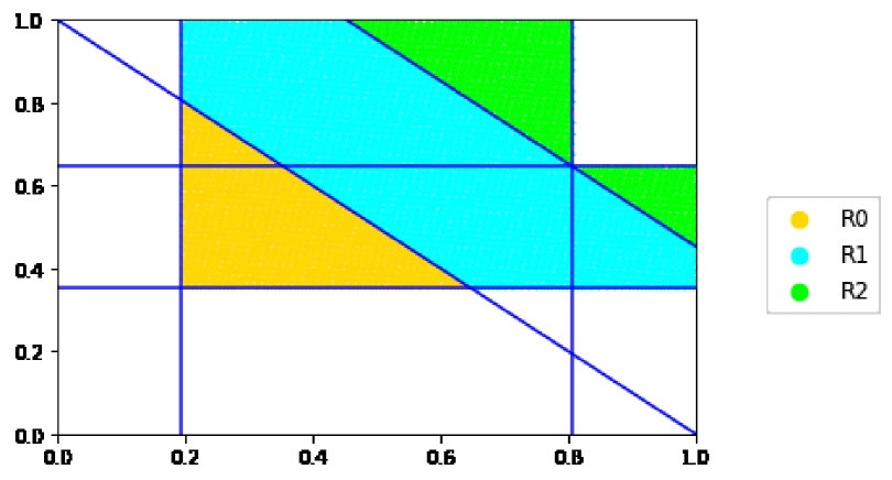
Figure 1: The regions $R_{0}$, $R_{1}$, and $R_{2}$ in the $uv$-plane representing the conditions given in Proposition 21 for the perturbation errors $c(n)-\widetilde{c}(n)$ to be equal to $0$, $1$, and $2$, respectively. The vertical boundary lines are given by the equations $u=\alpha$ and $u=1-\alpha$, the horizontal boundary lines are given by the equations $v=\beta$, $v=1-\beta$, and the two diagonal lines are given by $u+v=1$ and $u+v=1+\gamma$.

If $\alpha,\beta,1$ are linearly independent over $\mathbb{Q}$, then Weyl’s Theorem (Lemma 14) implies that the points $(u_{m},v_{m})$ are uniformly distributed in the unit square. By Lemma 17 and Proposition 21 it follows that, under this linear independence condition, the densities of the perturbation errors

$$P(d)=\lim_{N\to\infty}\frac{1}{N}\#\{n\leq N:c(n)-\widetilde{c}(n)=d\}$$ (48)

are given by $P(d)=A(R_{d})/A(R_{0}\cup R_{1}\cup R_{2})$, where $A(R)$ denotes the area of a region $R$. An elementary computation of the areas of the regions $R_{d}$ depicted in Figure 1 then yields

$$P(0) =\frac{\gamma}{2},\quad P(1)=1-\frac{\alpha^{2}+\beta^{2}+\gamma^{2}}{2\gamma},\quad P(2)=\frac{\alpha^{2}+\beta^{2}}{2\gamma}.$$

In particular, under the density conditions (34) of Theorem 4 and the above linear independence assumption, it follows all three densities are nonzero. Hence, under these conditions the perturbation errors $c(n)-\widetilde{c}(n)$ take on each of the values $0,1,2$ on a set of positive density.

6 Proof of Theorem 6

Let $\alpha$, $\beta$ and $\gamma$ be as in Theorem 6. Thus $\beta=\alpha$ and $\alpha$ and $\gamma$ are positive irrational numbers satisfying

$$2\alpha+\gamma=1.$$ (49)

In particular, we must have

$$\alpha<\frac{1}{2}.$$ (50)

Let $\widetilde{B_{\beta}}=(\widetilde{b}(n))_{n\in\mathbb{N}}$, where $\widetilde{b}(n)=b(n)-1$, and $\widetilde{B_{\gamma}}=\mathbb{N}\setminus(B_{\alpha}\cup\widetilde{B_{\beta}})=(\widetilde{c}(n))_{n\in\mathbb{N}}$ be the sequences defined in Theorem 6. Using (50), we see as in the proof of Theorem 4 that the sequences $B_{\alpha}$, $\widetilde{B_{\beta}}$, and $\widetilde{B_{\gamma}}$ form a partition of $\mathbb{N}$. The relations $b(n)-\widetilde{b}(n)=1$ and $\|\widetilde{b}-b\|=1$ follow directly from the definition of $\widetilde{b}(n)$. Thus, to complete the proof of Theorem 6 it remains to prove that

$$c(n)-\widetilde{c}(n)\in\{0,1\}.$$ (51)

This will follow from the three lemmas below.

We recall the notations (see (36) and (37))

$$E_{\gamma}(m)=\widetilde{B_{\gamma}}(m)-B_{\gamma}(m)$$

and

$$u_{m}=\{(m+1)\alpha\},\quad v_{m}=\{(m+1)\beta\},\quad w_{m}=1-\{u_{m}+v_{m}\}$$

from the proof of Theorem 4. We note that, by our assumption $\alpha=\beta$, we have

$$u_{m}=v_{m},\quad w_{m}=1-\{2u_{m}\}.$$ (52)

The first two lemmas are the special cases $\alpha=\beta$ (and thus $u_{m}=v_{m}$) of Lemma 16 and Lemma 18, respectively.

Lemma 22.

We have, for all $n\in\mathbb{N}$,

$$E_{\gamma}(m)=\begin{cases}1,&\text{if $1/2<u_{m}<1-\alpha$;}\\ 0,&\text{otherwise.}\end{cases}$$

Lemma 23.

We have, for all $n\in\mathbb{N}$,

$$c(n-1)\leq\widetilde{c}(n)\leq c(n).$$

The following lemma is a stronger version of Lemma 18, valid under the conditions of Theorem 6.

Lemma 24.

We have, for all $n\in\mathbb{N}$,

$$c(n)-1\leq\widetilde{c}(n)\leq c(n),$$

Proof.

The upper bound, $\widetilde{c}(n)\leq c(n)$, follows from Lemma 23. For the lower bound, suppose $\widetilde{c}(n)\leq c(n)-2$. Let $m=\widetilde{c}(n)$. Then

$$B_{\gamma}(m)\leq B_{\gamma}(m+1)\leq B_{\gamma}(c(n)-1)=n-1,$$

while

$$\widetilde{B_{\gamma}}(m+1)\geq\widetilde{B_{\gamma}}(m)=\widetilde{B_{\gamma}}(\widetilde{c}(n))=n.$$

Thus we have

$$E_{\gamma}(m)=\widetilde{B_{\gamma}}(m)-B_{\gamma}(m)\geq 1\text{ and }E_{\gamma}(m+1)=\widetilde{B_{\gamma}}(m+1)-B_{\gamma}(m+1)\geq 1.$$

By Lemma 22 this implies that

$$1/2<u_{m}<1-\alpha\text{ and }1/2<\{u_{m}+\alpha\}<1-\alpha.$$

The latter two relations imply

$$1/2<u_{m}<1-2\alpha,$$ (53)

and hence, by (49), $\gamma=1-2\alpha>1/2$. Therefore ${\lfloor 1/\gamma\rfloor}=1$, and by Lemma 10(iii) it follows that $c(n)-c(n-1)\in\{1,2\}$. Our assumption $\widetilde{c}(n)\leq c(n)-2$ and Lemma 23 then implies

$$c(n-1)=\widetilde{c}(n)=c(n)-2.$$

By Lemma 10(iv) it follows that, with $m=c(n-1)=\widetilde{c}(n)$, we have

$$w_{m}<\{1/\gamma\}\gamma=((1/\gamma)-1)\gamma=1-\gamma=2\alpha.$$ (54)

On the other hand, using (52) and (53) we have

$$w_{m}=1-\{2u_{m}\}=1-(2u_{m}-1)=2(1-u_{m})>2(2\alpha).$$ (55)

Comparing (54) and (55) yields $4\alpha<2\alpha$, which is a contradiction. Hence we must have $c(n)-\widetilde{c}(n)\in\{0,1\}$. This completes the proof of Lemma 24 and of Theorem 6. ∎

7 Proof of Theorem 1

The necessity of the condition (7) follows from the disjointness criterion of Lemma 13. Thus, it remains to show that if this condition is satisfied, then $\widetilde{B_{\gamma}}=\mathbb{N}\setminus(B_{\alpha}\cup B_{\beta})$ is an almost Beatty sequence satisfying the bounds (9), and that the upper bound here is attained for infinitely many $n$.

Suppose that $\alpha,\beta,\gamma$ are irrational numbers satisfying the conditions (6) and (7) of Theorem 1. Thus, there exist $r,s\in\mathbb{N}$ such that

$$r\alpha+s\beta=1.$$ (56)

We distinguish two cases: (I) $r=1$ or $s=1$, and (II) $r>1$ and $s>1$.

7.1 Proof of the error bounds (9), Case I: $r=1$ or $s=1$.

By symmetry it suffices to consider the case $r=1$. Then (56) reduces to $\alpha+s\beta=1$, and since $\gamma=1-\alpha-\beta>0$, we necessarily have $s\geq 2$ and

$$\gamma=(s-1)\beta.$$ (57)

Moreover, since $\beta=(1-\alpha)/s<1/2$, we have ${\lfloor(2-\beta)/(1-\beta)\rfloor}=2$ and therefore

$$\max\left(\left\lfloor\frac{2-\alpha}{1-\alpha}\right\rfloor,\left\lfloor\frac{2-\beta}{1-\beta}\right\rfloor\right)=\max\left(\left\lfloor 1+\frac{1}{1-\alpha}\right\rfloor,2\right)=1+\left\lfloor\frac{1}{1-\alpha}\right\rfloor.$$

Thus, to prove the desired bounds (9), it suffices to show that, for all $n\in\mathbb{N}$,

$$0\leq c(n)-\widetilde{c}(n)\leq\left\lfloor\frac{1}{1-\alpha}\right\rfloor+1.$$ (58)

Let

$$B_{s\beta}=({\lfloor n/(s\beta)\rfloor})_{n\in\mathbb{N}}$$ (59)

be the Beatty sequence of density $s\beta$. Since $\alpha+s\beta=1$, by Beatty’s theorem the sequences $B_{\alpha}$ and $B_{s\beta}$ partition $\mathbb{N}$.

Now observe that the sequence $B_{\beta}=({\lfloor n/\beta\rfloor})_{n\in\mathbb{N}}$ is the subsequence of $B_{s\beta}$ obtained by restricting the index $n$ in (59) to integers $n\equiv 0\bmod s$. Since $B_{\alpha}$ and $B_{s\beta}$ partition $\mathbb{N}$, it follows that

$$\widetilde{B_{\gamma}} =\mathbb{N}\setminus(B_{\alpha}\cup B_{\beta})=B_{s\beta}\setminus B_{\beta}=\{{\lfloor n/(s\beta)\rfloor}:n\in\mathbb{N},n\not\equiv 0\bmod s\}.$$

Hence $\widetilde{c}(m)$, the $m$th term of the sequence $\widetilde{B_{\gamma}}$, is equal to ${\lfloor n_{m}/(s\beta)\rfloor}$, where $n_{m}$ is the $m$th positive integer $n$ satisfying $n\not\equiv 0\bmod s$. A simple enumeration argument shows that if we represent $m$ (uniquely) in the form

$$m=i(s-1)+j,\quad i\in\{0,1,\dots\},\quad j\in\{1,2\dots,s-1\},$$

then $n_{m}=is+j$. With this notation, the $m$th term of $\widetilde{B_{\gamma}}$ is given by

$$\widetilde{c}(m)=\widetilde{c}(i(s-1)+j) ={\left\lfloor\frac{n_{m}}{s\beta}\right\rfloor}={\left\lfloor\frac{is+j}{s\beta}\right\rfloor}={\left\lfloor\frac{i}{\beta}+\frac{j}{s\beta}\right\rfloor}.$$ (60)

On the other hand, since, by (57), $c(n)={\lfloor n/\gamma\rfloor}={\lfloor n/((s-1)\beta)\rfloor}$, we have

$$c(m) ={\left\lfloor\frac{m}{(s-1)\beta}\right\rfloor}={\left\lfloor\frac{i(s-1)+j}{(s-1)\beta}\right\rfloor}={\left\lfloor\frac{i}{\beta}+\frac{j}{(s-1)\beta}\right\rfloor}.$$ (61)

From (60) and (61) we obtain, on using Lemma 9,

$$0 \leq c(m)-\widetilde{c}(m)={\left\lfloor\frac{i}{\beta}+\frac{j}{(s-1)\beta}\right\rfloor}-{\left\lfloor\frac{i}{\beta}+\frac{j}{s\beta}\right\rfloor}$$ (62)

$$={\left\lfloor\left(\frac{i}{\beta}+\frac{j}{(s-1)\beta}\right)-\left(\frac{i}{\beta}+\frac{j}{s\beta}\right)\right\rfloor}+\delta_{i,j}$$

$$\leq{\left\lfloor\frac{j}{s(s-1)\beta}\right\rfloor}+1\leq{\left\lfloor\frac{1}{s\beta}\right\rfloor}+1={\left\lfloor\frac{1}{1-\alpha}\right\rfloor}+1,$$

where

$$\delta_{i,j} =\delta\left(\left\{\frac{is+j}{s\beta}\right\},\left\{\frac{j}{s(s-1)\beta}\right\}\right)$$

$$=\begin{cases}1,&\text{if $\left\{\frac{is+j}{s\beta}\right\}+\left\{\frac{j}{s(s-1)\beta}\right\}\geq 1$;}\\ 0,&\text{otherwise.}\end{cases}$$

This proves the bounds (58).

7.2 Proof of the error bounds (9), Case II: $r>1$ and $s>1$.

In this case, we have $\gamma=1-\alpha-\beta=(r-1)\alpha+(s-1)\beta\geq\alpha+\beta$, so in particular

$$\gamma>1/2,\quad\alpha<1/2,\quad\beta<1/2.$$ (63)

Hence

$$\max\left(\left\lfloor\frac{2-\alpha}{1-\alpha}\right\rfloor,\left\lfloor\frac{2-\beta}{1-\beta}\right\rfloor\right)=2,$$

so the desired bounds (9) reduce to

$$0\leq c(n)-\widetilde{c}(n)\leq 2.$$ (64)

Now note that, by (63), we have $\gamma>\max(\alpha,\beta)$, so the conditions of Theorem 4 are satisfied. Moreover, since $B_{\alpha}$ and $B_{\beta}$ are disjoint, the sequence $\widetilde{B_{\beta}}$ defined in this theorem is identical to $B_{\beta}$, and consequently the sequences $\widetilde{B_{\gamma}}$ defined in Theorems 1 and 4 must also be equal. Hence, all results established in the proof of Theorem 4 can be applied in the current situation. In particular, Lemma 19 yields the desired bounds (64) for the perturbation errors $c(n)-\widetilde{c}(n)$.

7.3 Optimality of the error bounds (9)

To complete the proof of Theorem 1, it remains to show that the upper bounds in (9) are sharp.

Consider first Case I above, i.e., the case when $r=1$. In this case (9) reduces to (58), and we need to show that the upper bound in the latter inequality is attained infinitely often.

Consider integers $m\in\mathbb{N}$ satisfying $m\equiv 0\bmod(s-1)$. For such integers we have $j=s-1$ in the representation $m=i(s-1)+j$. Thus (62) reduces to

$$c(m)-\widetilde{c}(m)={\left\lfloor\frac{1}{s\beta}\right\rfloor}+\delta_{i,s-1}={\left\lfloor\frac{1}{1-\alpha}\right\rfloor}+\delta_{i,s-1},$$ (65)

where

$$\delta_{i,j}=\begin{cases}1,&\text{if $\left\{\frac{is+s-1}{s\beta}\right\}\geq 1-\left\{\frac{1}{s\beta}\right\}$;}\\ 0,&\text{otherwise.}\end{cases}$$

Note that $\{(is+(s-1))/(s\beta)\}=\{i\beta+\theta\}$ with $\theta=(s-1)/(s\beta)$. Since $\beta$ is irrational, by Weyl’s theorem (Lemma 14) the sequence $(\{i\beta\})_{i\in\mathbb{N}}$, and therefore also the shifted sequence $(\{i\beta+\theta\})_{i\in\mathbb{N}}$, is dense in $[0,1]$. Hence $\delta_{i,s-1}=1$ holds for infinitely many values of $i$. By (65) it follows that $c(m)-\widetilde{c}(m)={\lfloor 1/(1-\alpha)\rfloor}+1$ also holds for infinitely many $m$. This proves that the upper bound in (58) is attained for infinitely many $m$.

In Case II the bounds (9) reduce to $0\leq c(n)-\widetilde{c}(n)\leq 2$, and we need to show that $c(n)-\widetilde{c}(n)=2$ holds for infinitely many $n$. By Proposition 21 (which, as noted above, is applicable under the assumptions of Case II), $c(n)-\widetilde{c}(n)=2$ holds for infinitely many $n$ if and only if the conditions

$$\bigl{(}u_{m}<1-\alpha\text{ or }v_{m}<1-\beta\bigr{)}\text{ and }u_{m}+v_{m}>1+\gamma,$$ (66)

where $u_{m}=\{(m+1)\alpha\}$ and $v_{m}=\{(m+1)\beta\}$, hold for infinitely many $m$. Thus, it remains to show the latter assertion.

We may assume without loss of generality that $s>r$. (Note that the case $s=r$ is impossible since then (6) and (7) imply $\alpha+\beta=1/r$ and $\gamma=1-(\alpha+\beta)=1-1/r$, contradicting the irrationality of $\gamma$.) Under this assumption we have

$$\beta <\frac{1}{s}(r\alpha+s\beta)=\frac{1}{s},$$

$$\gamma =1-\alpha-\beta<1-\frac{1}{s}(r\alpha+s\beta)=1-\frac{1}{s}.$$

In view of these bounds, a sufficient condition for (66) is

$$u_{m}\in(1-\epsilon_{1},1),\quad v_{m}\in\left(1-\frac{1}{s},1-\frac{1}{s}+\epsilon_{2}\right),$$ (67)

provided $\epsilon_{1},\epsilon_{2}>0$ are small enough. Indeed, if $\beta<(1/s)-\epsilon_{2}$ and $\gamma<1-(1/s)-\epsilon_{1}$, then the upper bound for $v_{m}$ in (67) implies $v_{m}<1-\beta$, while the lower bounds for $u_{m}$ and $v_{m}$ imply $u_{m}+v_{m}>2-(1/s)-\epsilon_{1}>1+\gamma$. Thus it remains to show that, given arbitrarily small $\epsilon_{1}$ and $\epsilon_{2}$, there exist infinitely many $m$ satisfying (67).

By (7) we have $\beta=(1-r\alpha)/s$ and hence

$$v_{m}=\{\beta(m+1)\}=\left\{\frac{m+1}{s}-r\frac{\alpha(m+1)}{s}\right\}.$$ (68)

Setting

$$u_{m}^{*}=\left\{\frac{\alpha(m+1)}{s}\right\}$$

and letting $j\in\{1,2,\dots,s\}$ be defined by

$$m+1\equiv j\bmod s,$$

we can write (68) as

$$v_{m} =\left\{\frac{j}{s}-r\frac{\alpha(m+1)}{s}\right\}=\left\{\frac{j}{s}-r\left\{\frac{\alpha(m+1)}{s}\right\}\right\}$$ (69)

$$=\left\{\frac{j}{s}-ru_{m}^{*}\right\}=1-\left\{ru_{m}^{*}-\frac{j}{s}\right\}.$$

Let $0<\epsilon<1$ be given, and suppose that $m$ satisfies

$$m+1\equiv r-1\bmod s$$ (70)

and

$$u_{m}^{*}\in\left(\frac{1-\epsilon}{s},\frac{1}{s}\right).$$ (71)

Then

$$u_{m} =\left\{s\frac{\alpha(m+1)}{s}\right\}=\left\{s\left\{\frac{\alpha(m+1)}{s}\right\}\right\}=\{su_{m}*\}\in(1-\epsilon,1).$$ (72)

Moreover, if $\epsilon<1/r$, then (69) with $j=r-1$ implies

$$v_{m} =1-\left\{ru_{m}^{*}-\frac{r-1}{s}\right\}=1-\left\{\frac{1}{s}+r\left(u_{m}^{*}-\frac{1}{s}\right)\right\}\in\left(1-\frac{1}{s},1-\frac{1}{s}+\frac{r\epsilon}{s}\right).$$ (73)

From (72) and (73) we see that the (67) holds with $\epsilon_{1}$ and $\epsilon_{2}$ given by

$$\epsilon_{1}=\epsilon,\quad\epsilon_{2}=\frac{r\epsilon}{s}.$$ (74)

Hence, if $\epsilon$ is chosen small enough, then for any $m$ satisfying the conditions (70) and (71), the desired bounds (66) hold.

It remains to show that there are infinitely many $m$ satisfying these two conditions. The first of these conditions, (70), restricts $m$ to integers of the form $m=is+r-2$, $i=0,1,2,\dots$. For such $m$ we have

$$u_{m}^{*}=\left\{\frac{\alpha(m+1)}{s}\right\}=\left\{\frac{\alpha(is+r-1)}{s}\right\}=\left\{\alpha i+\frac{(r-1)\alpha}{s}\right\}.$$

Since $\alpha$ is irrational, by Weyl’s theorem (Lemma 14), the sequence $(\{\alpha i\})_{i\geq 0}$, and hence also the sequence $(\{\alpha i+((r-1)\alpha/s)\})_{i\geq 0}=(u^{*}_{is+r-2})_{i\geq 0}$, is dense in $[0,1]$. Thus there exist infinitely many $m$ for which $u_{m}^{*}$ falls into the interval $((1-\epsilon)/s,1/s)$, i.e., satisfies (71). This proves our claim and completes the proof of Theorem 1.

Remark 25.

The above argument yields the maximal value taken on by the perturbation errors $c(n)-\widetilde{c}(n)$. One can ask, more generally, for the exact set of values taken on by these errors, and for the densities with which these values occur. This is a more difficult problem that leads to some very delicate questions on the behavior of the pairs $(u_{m},v_{m})$. We plan to address this question in a future paper. We note here only that, in general, it is not the case that the perturbation errors $c(n)-\widetilde{c}(n)$ are uniformly distributed over their range of possible values.

8 Proof of Theorem 8

Let $\alpha,\beta,\gamma$ satisfy the conditions of the theorem; that is, assume that $\alpha,\beta,\gamma$ are positive irrational numbers summing to $1$ and suppose in addition that $\alpha>1/3$ and that the numbers $1,\alpha,\beta$ are linearly independent over $\mathbb{Q}$.

We will show that, under these assumptions, there exist infinitely many $m\in\mathbb{N}$ such that

$$m\in B_{\alpha},\quad m+1\in B_{\beta}\cap B_{\gamma},\quad m+2\in B_{\alpha}.$$ (75)

The desired conclusion follows from (75). Indeed, for any $m$ satisfying (75) the element $m+1$ belongs to both $B_{\beta}$ and $B_{\gamma}$. Thus, in order to obtain a partition of the desired type (i.e., of the form $\mathbb{N}=B_{\alpha}\cup\widetilde{B_{\beta}}\cup\widetilde{B_{\gamma}}$), for one of these latter two sequences the element $m+1$ would have to “perturbed” to avoid the overlap. However, since $m$ and $m+2$ are elements of $B_{\alpha}$, a perturbation of $m+1$ by $\pm 1$ creates an overlap with an element in $B_{\alpha}$, in contradiction to the partition property. Thus there does not exist a partition $\mathbb{N}=B_{\alpha}\cup\widetilde{B_{\beta}}\cup\widetilde{B_{\gamma}}$ in which the perturbation errors for the almost Beatty sequences $\widetilde{B_{\beta}}$ and $\widetilde{B_{\gamma}}$ are bounded by $1$ in absolute value.

It remains to show that (75) holds for infinitely many $m$. We distinguish two cases, $1/3<\alpha<1/2$ and $1/2<\alpha<1$.

Suppose first that

$$1/3<\alpha<1/2.$$ (76)

Without loss of generality, we may assume that $\beta\leq\gamma$, which, by (76), implies

$$\beta\leq\frac{1}{2}(\beta+\gamma)=\frac{1}{2}(1-\alpha)<\frac{1}{3}<\alpha.$$ (77)

Applying part (i) of Lemma 10 we obtain

$$m+1\in B_{\beta}\cap B_{\gamma}\Longleftrightarrow\{(m+1)\beta\}>1-\beta\text{ and }\{(m+1)\gamma\}>1-\gamma.$$ (78)

Using the notation (cf. (30) and (31))

$$u_{m} =\{(m+1)\alpha\},\ v_{m}=\{(m+1)\beta\},\ w_{m}=\{(m+1)\gamma\}=1-\{u_{m}+v_{m}\},$$

and the relation $\gamma=1-\alpha-\beta$, the two conditions on the right of (78) are seen to be equivalent to

$$v_{m} >1-\beta,$$ (79)

$$\{u_{m}+v_{m}\} <1-\alpha-\beta,$$ (80)

respectively.

Next, by part (iv) of Lemma 10 along with our assumption (76) (which implies that the number $k$ in Lemma 10(iv) is equal to ${\lfloor 1/\alpha\rfloor}=2$) we have

$$m\in B_{\alpha}\text{ and }m+2\in B_{\alpha}\Longleftrightarrow\{1/\alpha\}\alpha<u_{m}<\alpha.$$ (81)

Since $\{1/\alpha\}\alpha=((1/\alpha)-2)\alpha=1-2\alpha$, the condition on the right of (81) is equivalent to

$$1-2\alpha<u_{m}<\alpha.$$ (82)

Thus $m$ satisfies (75) if and only if the numbers $u_{m}$ and $v_{m}$ satisfy (79), (80), and (82), and it remains to show that the latter three conditions hold for infinitely many $m$. To this end, let $\epsilon>0$ be given and consider the intervals

$$I_{\epsilon}=(\alpha-\epsilon,\alpha),\quad J_{\epsilon}=(1-\beta,1-\beta+\epsilon).$$

If $\epsilon$ is sufficiently small, then, since $1-2\alpha<\alpha$ by (76), we have

$$I_{\epsilon}\subset(1-2\alpha,\alpha),\quad J_{\epsilon}\subset(1-\beta,1).$$ (83)

Moreover, our assumption (77) implies $\alpha-\epsilon+(1-\beta)>1$ provided $\epsilon$ is sufficiently small, and hence

$$I_{\epsilon}+J_{\epsilon}\subset(\alpha+1-\beta-\epsilon,\alpha+1-\beta+\epsilon)\subset(1,2),$$ (84)

where $I+J$ denotes the sumset of $I$ and $J$, i.e., the set of all elements $x+y$ with $x\in I$ and $y\in J$.

Assume now that $\epsilon$ is small enough so that (83) and (84) both hold. Let $(u_{m},v_{m})$ be such that

$$u_{m}\in I_{\epsilon}\text{ and }v_{m}\in J_{\epsilon}.$$ (85)

Then, by (83), (82) and (79) are satisfied. Moreover, in view of (84), we have

$$\{u_{m}+v_{m}\}=u_{m}+v_{m}-1<\alpha+(1-\beta+\epsilon)-1=\alpha-\beta+\epsilon,$$ (86)

and since $\alpha<1/2$, we have $\alpha+\epsilon<1/2<1-\alpha$ provided $\epsilon<(1/2)-\alpha$. Hence, for sufficiently small $\epsilon$, the right-hand side of (86) is smaller than $1-\alpha-\beta$, and condition (80) is satisfied as well.

Thus, assuming $\epsilon$ is sufficiently small, any pair $(u_{m},v_{m})$ for which (85) holds satisfies the three conditions (79), (80), and (82). Since $(u_{m},v_{m})=(\{(m+1)\alpha\},\{(m+1)\beta\})$ and, by assumption, the numbers $1,\alpha,\beta$ are linearly independent over $\mathbb{Q}$, the two-dimensional version of Weyl’s Theorem (Lemma 14(ii)) guarantees that there are infinitely many such pairs. This completes the proof of the theorem in the case when $1/3<\alpha<1/2$.

Now suppose $1/2<\alpha<1$. As before, the condition $m+1\in B_{\beta}\cap B_{\gamma}$ in (75) is equivalent to the two conditions (79) and (80). However, the remaining condition in (75), “$m\in B_{\alpha}$ and $m+2\in B_{\alpha}$”, requires a slightly different treatment in the case when $\alpha>1/2$. In this case, the number $k$ in Lemma 10(iv) is equal to $k={\lfloor 1/\alpha\rfloor}=1$ and we have $\{1/\alpha\}\alpha=1-\alpha$. Hence, by Lemma 10(iv) a sufficient condition for $m\in B_{\alpha}$ and $m+2\in B_{\alpha}$ to hold is

$$u_{m}<1-\alpha.$$ (87)

The latter condition is the analog of (82), which characterizes the integers $m$ satisfying “$m\in B_{\alpha}$ and $m+2\in B_{\alpha}$” in the case when $1/3<\alpha<1/2$.

The remainder of the argument parallels that for the case $1/3<\alpha<1/2$. We seek to show that there exist infinitely many $m$ such that (79), (80), and (87) hold. Given $\epsilon>0$, set

$$I_{\epsilon}^{\prime}=(\beta,\beta+\epsilon),\quad J_{\epsilon}=(1-\beta,1-\beta+\epsilon).$$

If $\epsilon$ is sufficiently small, then, since $\beta=1-\alpha-\gamma<1-\alpha$, we have

$$I_{\epsilon}^{\prime}\subset(0,1-\alpha)\quad J_{\epsilon}\subset(1-\beta,1),$$ (88)

and

$$I_{\epsilon}^{\prime}+J_{\epsilon}\subset(1,2).$$ (89)

From (88) we immediately see that (79) and (87) hold whenever $u_{m}\in I_{\epsilon}^{\prime}$ and $v_{m}\in J_{\epsilon}$. Moreover, by (89) we have, for any sufficiently small $\epsilon$,

$$\{u_{m}+v_{m}\}=u_{m}+v_{m}-1<(\beta+\epsilon)+(1-\beta+\epsilon)-1=2\epsilon<1-\alpha-\beta,$$ (90)

so (80) holds as well whenever $u_{m}\in I_{\epsilon}^{\prime}$ and $v_{m}\in J_{\epsilon}$. As before, Weyl’s Theorem ensures that there are infinitely many $m$ for which the latter two conditions hold, and hence infinitely many $m$ for which (85) holds. This completes the proof of Theorem 8.

9 Concluding Remarks

In this section we discuss some related results in the literature, other approaches to almost Beatty partitions, possible extensions and generalizations of our results, and directions for future research.

More on iterated Beatty partitions.

In Theorem 3 we constructed almost Beatty partitions by iterating the standard two-part Beatty partition process. This is perhaps the most natural approach to partitions into more than two “Beatty-like” sequences, and many special cases of such constructions have appeared in the literature. Skolem observed in 1957 [24, p. 68] that starting out with the complementary Beatty sequences $({\lfloor n\Phi\rfloor})_{n\in\mathbb{N}}$ and $({\lfloor n\Phi^{2}\rfloor})_{n\in\mathbb{N}}$ and “partitioning” the index $n$ in the first sequence into the same pair of complementary Beatty sequences yields a three part partition consisting of the sequences $({\lfloor\Phi{\lfloor\Phi n\rfloor}\rfloor})_{n\in\mathbb{N}}$, $({\lfloor\Phi{\lfloor\Phi^{2}n\rfloor}\rfloor})_{n\in\mathbb{N}}$, and $({\lfloor\Phi^{2}n\rfloor})_{n\in\mathbb{N}}$. Further iterations of this process lead to partitions into arbitrarily many Beatty-like sequences involving the golden ratio or other special numbers; see, for example, Fraenkel [8, 9, 10], Kimberling [15], and Ballot [2].

The “iterated Beatty partition” approach leads to sequences whose terms are given by iterated floor functions. Removing all but the outermost floor function in such a sequence, one obtains an exact Beatty sequence whose terms differ from the original sequence by a bounded quantity. Thus, the partitions generated by this approach are almost Beatty partitions in the sense defined of this paper. However, as our results show, these partitions do not necessarily yield the smallest perturbation errors.

Partitions into non-homogeneous Beatty sequences.

Another natural approach to almost Beatty partitions is by considering non-homogeneous Beatty sequences, that is, sequences of the form $({\lfloor(n+\beta)/\alpha\rfloor})_{n\in\mathbb{N}}$. Clearly, any sequence of this form differs from the exact Beatty sequence $({\lfloor n/\alpha\rfloor})_{n\in\mathbb{N}}$ by a bounded amount, and hence is an almost Beatty sequence. Thus, any partition of $\mathbb{N}$ into non-homogeneous Beatty sequences is a partition into almost Beatty sequences. The question of when a partition of $\mathbb{N}$ into $k$ non-homogeneous Beatty sequences exists has received considerable attention in the literature, but a complete solution is only known in the case $k=2$; see, for example, Fraenkel [7] and O’Bryant [21] for the case $k=2$, and Tijdeman [28] and the references therein for the general case. An intriguing question is whether any of the sequences constructed in Theorems 1–6 can be represented as a non-homogeneous Beatty sequence.

Very recently, Allouche and Dekking [1] considered two- and three-part partitions of $\mathbb{N}$ into sequences of the form $(p{\lfloor\alpha n\rfloor}+qn+r)_{n\in\mathbb{N}}$, where $p,q,r$ are integers and $\alpha$ is an irrational number. Such sequences can be viewed as generalized non-homogeneous Beatty sequences, and they represent almost Beatty sequences in the sense of this paper, associated with the exact Beatty sequence $({\lfloor(p\alpha+q)n\rfloor})_{n\in\mathbb{N}}$. Again, it would be interesting to see if any of the sequences constructed in our partitions are of the above form.

Other approximation measures.

In our results we measured the “closeness” of two sequences $A=(a(n))_{n\in\mathbb{N}}$ and $B=(b(n))_{n\in\mathbb{N}}$ by the sup-norm $\|a-b\|$. This norm has the natural interpretation as the maximal amount by which an element in one sequence needs to be “perturbed” in order to obtain the corresponding element in the other sequence. An alternative, and seemingly equally natural, measure of closeness of two sequences $A$ and $B$ is the sup-norm of the associated counting functions, i.e.,

$$\|A-B\|=\sup\{|A(n)-B(n)|:n\in\mathbb{N}\}.$$

One can ask how our results would be affected if the approximation errors had been measured in terms of the latter norm. Surprisingly, this question has a trivial answer, at least in the case of Theorems 1, 4, and 6: In all of these cases, we have $\|B_{\beta}-\widetilde{B_{\beta}}\|\leq 1$ and $\|B_{\gamma}-\widetilde{B_{\gamma}}\|\leq 1$ whenever the conditions of the theorems are satisfied. In other words, when measured by the counting function norm, the almost Beatty sequences constructed in these theorems are either exact Beatty sequences or just one step away from being an exact Beatty sequence. This follows easily from Lemmas 12, 15, and 16. The reason for the simple form of this result is that the counting function norm is a much less sensitive measure than the element-wise norm we have used in this paper.

Partitions into $n$ almost Beatty sequences.

A natural question is whether the constructions of Theorems 3–6 can be generalized to yield partitions of $\mathbb{N}$ into more than three almost Beatty sequences. The “iterated Beatty partition” approach in Theorem 3 lends itself easily to such a generalization, though it is not clear what the best-possible perturbation errors are that can be achieved in the process.

Densities of perturbation errors.

Another question concerns the densities with which the perturbation errors in our results occur. We have computed these densities in the case of Theorem 4 under an appropriate linear independence assumption (see the end of Section 5), but in the case of Theorem 1 this would be a much more difficult undertaking (see Remark 25). One motivation for computing these densities is that we can then consider a refined approximation measure given by the weighted average of the absolute values of the errors, with the weights being the associated densities. It would be interesting to see which approaches yield the closest approximation to a partition into Beatty sequences in terms of this refined measure of closeness.

Connection with optimal assignment problems.

Finally we remark on an interesting connection with a class of problems involving the assignment or scheduling of tasks in a manner that is, in an appropriate sense, most efficient or most fair. Problems of this type arise in many contexts, from distributing tasks among different machines, to allocating seats in an election, to assigning drivers in a carpool; see, for example, Coppersmith et al. [6].

We describe one such problem, the chairman assignment problem of Tijdeman [27]: Suppose $k$ states with weights $\lambda_{1},\dots,\lambda_{k}$, where the $\lambda_{i}$ are positive real numbers satisfying $\sum_{i=1}^{k}\lambda_{i}=1$, form a union. Each year one of the states is chosen to designate the chair of the union. The goal is to perform this assignment in such way that, at any time, the proportion of chairs chosen from a given state up to that time is as close as possible to the weight of that state. In his paper, Tijdeman determines an assignment that is optimal in a certain global sense, and he gives a recursive algorithm to compute the optimal assignment sequence.

Mathematically, an assignment of chairs amounts to a partition of the positive integers into $k$ sets. Partitions into $k$ almost Beatty sequences with densities given by the weights $\lambda_{i}$ of the states provide natural candidates for a “fair” assignment. In particular, any of the partitions produced by Theorems 1–6 yields a possible chair assignment sequence for the case of three states with weights $\alpha$, $\beta$, and $\gamma$. These partitions turn out to be different from those given by Tijdeman, and they are not optimal with respect to the measure used by Tijdeman (which essentially amounts to minimizing the discrepancies $\sup_{n}|A_{i}(n)-\lambda_{i}n|$, where $A_{i}$ is the $i$th set in the partition). However, as shown in this paper, these partitions are, in many cases, best-possible in a different sense and thus might be of interest in applications to assignment problems. Exploring these connections and applications further could be a fruitful area for future research.

10 Acknowledgments

This work originated with an undergraduate research project carried out in Spring 2018 at the Illinois Geometry Lab at the University of Illinois; we thank the IGL for providing this opportunity. We also thank Michel Dekking for calling our attention to the paper [1] and the editor-in-chief for referring us to Tijdeman’s paper [27] on the chairman assignment problem.

 

2010 Mathematics Subject Classification: Primary 11B83; Secondary 05A17, 11P81.

Keywords: Beatty sequence, complementary sequence, partition of the integers.

 

(Concerned with sequences A000201, A003144, A003145, A003146, A003623, A004919, A004976, A158919, A277722, A277723, and A277728.)

 

Received October 5 2018; revised version received July 3 2019. Published in Journal of Integer Sequences, July 7 2019.

 

Return to Journal of Integer Sequences home pagehttp://www.cs.uwaterloo.ca/journals/JIS/.

References

- [1] J. P. Allouche and F. M. Dekking, Generalized Beatty sequences and complementary triples, preprint, 2018. Available at https://arXiv.org/abs/1809.03424.
- [2] C. Ballot, On functions expressible as words on a pair of Beatty sequences, J. Integer Sequences 20 (2017), Article 17.4.2.
- [3] T. Bang, On the sequence . Supplementary note to the preceding paper by Th. Skolem, Math. Scand. 5 (1957), 69–76.
- [4] S. Beatty, Problem 3173, Amer. Math. Monthly 33 (1926), 159.
- [5] L. E. Bush, The William Lowell Putnam Mathematical Competition, Amer. Math. Monthly 68 (1961), 18–33.
- [6] D. Coppersmith, T. J. Nowicki, G. A. Paleologo, C. Tresser, and C. W. Wu, The optimality of the online greedy algorithm in carpool and chairman assignment problems, ACM Trans. Algorithms 7 (2011), Art. 37.
- [7] A. S. Fraenkel, The bracket function and complementary sets of integers, Canad. J. Math. 21 (1969), 6–27.
- [8] A. S. Fraenkel, Complementary systems of integers, Amer. Math. Monthly 84 (1977), 114–115.
- [9] A. S. Fraenkel, Iterated floor function, algebraic numbers, discrete chaos, Beatty subsequences, semigroups, Trans. Amer. Math. Soc. 341 (1994), 639–664.
- [10] A. S. Fraenkel, Complementary iterated floor words and the Flora game, SIAM J. Discrete Math. 24 (2010), 570–588.
- [11] Y. Ginosar and I. Yona, A model for pairs of Beatty sequences, Amer. Math. Monthly 119 (2012), 636–645.
- [12] R. L. Graham, On a theorem of Uspensky, Amer. Math. Monthly 70 (1963), 407–409.
- [13] A. Holshouser and H. Reiter, A generalization of Beatty’s theorem, Southwest J. Pure Appl. Math. (2001), 24–29.
- [14] K. S. Kedlaya, B. Poonen, and R. Vakil, The William Lowell Putnam Mathematical Competition, 1985–2000, Mathematical Association of America, 2002.
- [15] C. Kimberling, Complementary equations and Wythoff sequences, J. Integer Sequences 11 (2008), Article 08.3.3.
- [16] C. Kimberling and K. B. Stolarsky, Slow Beatty sequences, devious convergence, and partitional divergence, Amer. Math. Monthly 123 (2016), 267–273.
- [17] L. F. Klosinski, G. L. Alexanderson, and L. C. Larson, The Fifty-Sixth William Lowell Putnam Mathematical Competition, Amer. Math. Monthly 103 (1996), 665–677.
- [18] L. Kuipers and H. Niederreiter, Uniform Distribution of Sequences, Wiley-Interscience, 1974.
- [19] I. Niven, Diophantine Approximations, Dover Publications, 2008.
- [20] K. O’Bryant, A generating function technique for Beatty sequences and other step sequences, J. Number Theory 94 (2002), 299–319.
- [21] K. O’Bryant, Fraenkel’s partition and Brown’s decomposition, Integers 3 (2003), A11.
- [22] Lord Rayleigh, The Theory of Sound, Macmillan, 1894.
- [23] I. J. Schoenberg, Mathematical Time Exposures, Mathematical Association of America, 1982.
- [24] T. Skolem, On certain distributions of integers in pairs with given differences, Math. Scand. 5 (1957), 57–68.
- [25] N. J. A. Sloane, The On-Line Encyclopedia of Integer Sequences, 2018. Published electronically at https://oeis.org.
- [26] K. B. Stolarsky, Beatty sequences, continued fractions, and certain shift operators, Canad. Math. Bull. 19 (1976), 473–482.
- [27] R. Tijdeman, The chairman assignment problem, Discrete Math. 32 (1980), 323–330.
- [28] R. Tijdeman, Exact covers of balanced sequences and Fraenkel’s conjecture, in Algebraic Number Theory and Diophantine Analysis (Graz, 1998), de Gruyter, 2000, pp. 467–483.
- [29] J. V. Uspensky, On a problem arising out of the theory of a certain game, Amer. Math. Monthly 34 (1927), 516–521.