Forward-backward multiplicity fluctuations in ultra-relativistic nuclear collisions
with wounded quarks and fluctuating strings

Abstract

We analyze a generic model where wounded quarks are amended with strings in which both end-point positions fluctuate in spatial rapidity. With the assumption that the strings emit particles independently of one another and with a uniform distribution in rapidity, we are able to analyze the model semi-analytically, which allows for its detailed understanding. Using as a constraint the one-body string emission functions obtained from the experimental data for collisions at $\sqrt{s_{NN}}=200$ GeV, we explore the two-body correlations for various scenarios of string fluctuations. We find that the popular measures used to quantify the longitudinal fluctuations ($a_{nm}$ coefficients) are limited with upper and lower bounds. These measures can be significantly larger in the model where both end-point are allowed to fluctuate, compared to the model with single end-point fluctuations.

I Introduction

The purpose of this paper is to present a detailed semi-analytic analysis of models of ultra-relativistic nuclear collisions where the early production of particles occurs from strings. The strings are associated with wounded quarks, and both of their end-point positions fluctuate in spatial rapidity. The model generalizes the analysis of Broniowski and Bożek (2016) where only one-end fluctuations were considered. The main assumptions are that the strings emit particles independently of one another and that the production from a string is uniform between its end-points. We obtain the one-body string emission function from a fit to the experimental data at $\sqrt{s_{NN}}=200$ GeV, and use it to constrain the freedom in the distribution of the end-point positions. We then explore in detail the two-body correlations in various scenarios for the fluctuating end-points. The derived analytic formulas allow for a full understanding of this simple model. In particular, we show that standard measures applied in analyses of the longitudinal fluctuations, such as the Legendre $a_{nm}$ coefficients, fall between certain bounds. This explains why a priori different models may provide quite similar results for these measures of the longitudinal correlations. We find that the $a_{nm}$ coefficients can be significantly larger (by a factor of $\sim 3$) when one allows for two end-point to fluctuate, compared to the case of single end-point fluctuations of Broniowski and Bożek (2016). This observation is relevant for phenomenological studies. Since the model, despite its simplifications, is generic, sharing features with more complicated string implementations, our findings shed light on correlations from other string models in application to ultra-relativistic heavy-ion collisions.

The basic phenomenon explored in this paper and illustrated with definite calculations can be understood in very simple terms. Consider a string with left and right end-points and an acceptance window in pseudorapidity. If the left end-point were always left of the acceptance window, and the right end-point to the right (they may fluctuate or not, but cannot enter the window), then the string seen in the window is always the same, hence no fluctuations occur. If, however, an endpoint via fluctuation enters the acceptance window, then fluctuations occur, as its observed fragment may be shorter or longer. The fluctuation effect is larger when both end-points fluctuate into the acceptance window, which is the case explored in detail below.

The concept of wounded sources formed in the initial stages of ultra-relativistic heavy-ion collisions has proven to be phenomenologically successful in reproducing multiplicity distributions from soft particle production. The idea (see Białas (2008) for a discussion of the foundations), adopts the Glauber model Glauber in its variant suitable for inelastic collisions Czyż and Maximon (1969). Whereas the wounded nucleon scaling Białas et al. (1976), when applied to the highest BNL Relativistic Heavy-Ion Collider (RHIC) or the CERN Large Hadron Collider (LHC) energies, requires a sizable admixture of binary collisions Back et al. (2002); Kharzeev and Nardi (2001), the scaling based on wounded quarks Białas et al. (1977a, b); Białas and Czyż (1979); Anisovich et al. (1978) works remarkably well Eremin and Voloshin (2003); Kumar Netrakanti and Mohanty (2004); Białas and Bzdak (2007, 2008); Alver et al. (2008); Agakishiev et al. (2012); Adler et al. (2014); Loizides et al. (2014); Adare et al. (2016); Lacey et al. (2016); Bożek et al. (2016); Zheng and Yin (2016); Sarkisyan et al. (2016); Mitchell et al. (2016); Chaturvedi et al. (2016); Loizides (2016); Tannenbaum (2017). Another successful approach Zakharov (2016, 2017) amends the wounded nucleons with a meson-cloud component.

For mid-rapidity production, the wounded quark scaling takes the simple form

$$N_{\rm ch}=k(\langle N_{A}\rangle+\langle N_{B}\rangle),$$ (1)

where $N_{\rm ch}$ is the number of charged hadrons in a mid-rapidity bin, and $\langle N_{i}\rangle$ are the average numbers of wounded quarks in nucleus $i$ in a considered centrality class. The proportionality constant $k$ should not depend on centrality or the mass numbers of the nuclei (i.e., on the overall number of participants), and indeed this requirement is satisfied to expected accuracy Bożek et al. (2016); Tannenbaum (2017). Of course, $k$ increases with the collision energy.

When it comes to modeling the rapidity spectra, formula (1) is replaced with

$$\frac{dN}{d\eta}=\langle N_{A}\rangle f(\eta)+\langle N_{B}\rangle f(-\eta),$$ (2)

where $f(\eta)$ is a universal (at a given collision energy) profile for emission from a wounded quark (we adopt the convention that nucleus $A$ moves to the right and $B$ to the left). For symmetric ($A=B$) collisions one only gets access to the the symmetric part of $f(\eta)$, as then $\langle N_{A}\rangle=\langle N_{B}\rangle$. However, from asymmetric collisions, such as d-Au, one can also extract the antisymmetric component in the wounded nucleon Białas and Czyż (2005) or wounded quark model Barej et al. (2018); Adare et al. (2018) (for A-A collisions analogous analyses were carried out in Gaździcki and Gorenstein (2006); Bzdak and Woźniak (2010); Bzdak (2009)), with the finding that $f(\eta)$ is peaked in the forward region, thus quite naturally emission is in the forward direction. However, $f(\eta)$ is widely spread in the whole kinematically available range. The phenomenological result of the approximate triangular shape of the emission profile was later used in modeling the initial conditions for further evolution, see e.g. Adil et al. (2006); Bożek and Wyskiel (2010); Bożek and Broniowski (2013); Monnai and Schenke (2016); Chatterjee and Bożek (2017).

Microscopically, the approximate triangular shape of the emission function finds a natural origin in color string models, where one end-point of the string is fixed, whereas the location of the other end-point fluctuates. In particular, in the basic Brodsky-Gunion-Kuhn mechanism Brodsky et al. (1977), the emission proceeds from strings in which one end-point is associated with a valence parton, and the other end-point, corresponding to wee partons, is randomly generated along the space-time rapidity $\eta$. When the distribution of the fluctuating end-point is uniform in $\eta$, and so is the string fragmentation distribution, then the triangular shape for the emission function follows.

Various Monte Carlo codes implementing the Lund string formation and decays (see, e.g., Andersson et al. (1983); Wang and Gyulassy (1991); Lin et al. (2005); Sjöstrand et al. (2015); Bierlich et al. (2018); Ferreres-Solé and Sjöstrand (2018)) or the dual parton model/Regge-exchange approach Capella et al. (1994); Werner et al. (2010); Pierog et al. (2015) also introduce strings of fluctuating ends, with various specific mechanisms and effects (baryon stopping, nuclear shadowing) additionally incorporated. Apart from reproducing the measured one-body spectra, achieved by appropriate tune-ups of parameters, the incorporated initial-state correlations show up in event-by-event fluctuations that can be accessed experimentally. Thus the fluctuating strings are standard objects used in modeling the early phase of high-energy reactions.

Our model joins the concept of wounded sources with strings in the following way:

1. Each wounded source has an associated string.

2. The strings emit particles independently of each-other.

3. The end-points of a string are generated universally (in the same manner for all wounded objects) from appropriate distributions.

4. The emission of particles from a string occurring between the end-points is homogeneous in spatial rapidity.

In such a model, event-by-event fluctuations take the origin from fluctuations of the number of wounded objects, as well as from fluctuations of the positions of the end points Broniowski and Bożek (2016). The goal of this paper is to study this generic model, with the focus on the end-point behavior which probes the underlying physics. We take a general approach, with no prejudice as to how the end-points are fluctuating, but using the one-body emission profiles obtained from experiment as a physical constraint.

More complicated mechanisms associated with dense systems, such as the formation of color ropes Biro et al. (1984); Sorge (1995) or nuclear shadowing, are not incorporated in our picture. Also, we consider one type of strings, which allows for simple analytic derivations.

We remark that associating a string with a leading quark is in the spirit of the Lund approach (cf. discussion of Sec. 5 in Andersson et al. (1983)). So for simplicity we have in each event $N_{i}$ “wounded strings” associated with valence quarks in nucleus $i$. Other more complicated choices (e.g, including the binary collisions) are also possible here, but the advantage of our prescription is that by definition it complies with the experimental scaling of multiplicities of Eq. (1).

A specific implementation of some ideas explored in this work, with strings that have one end fixed and the other fluctuating, has been presented in Broniowski and Bożek (2016).

The outline of our paper is as follows:

In Sec. II we use the rapidity spectra from d-Au and Au-Au reactions at $\sqrt{s_{NN}}=200$ GeV to obtain the one-body emission profile of the wounded quark. In Sec. III we explore our generic string model and derive simple relations between string end-point distributions and n-body-emission profiles for the radiation from individual strings. Section IV discusses how a given one-body-emission profile can correspond to a family of different functions for the string end-point distributions. Two-body correlations from a single string are discussed in Sec. V, whereas in Sec. VI they are combined to form the two-body correlations in nuclear collisions. Section VII presents the Legendre $a_{nm}$ coefficients of the two-particle correlations. Finally, Sec. VIII draws the final conclusions from our work. Some more technical developments can be found in the appendices.

II Emission profiles from wounded quarks

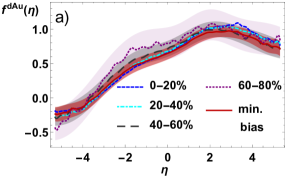
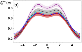
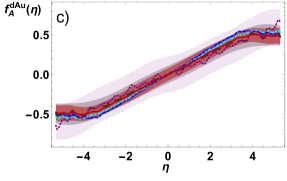
Figure 1: One-particle emission profiles obtained in the wounded quark model via Eqs. (2-4) from the PHOBOS rapidity spectra for d-Au collisions at $\sqrt{s_{NN}}=200$ GeV Back et al. (2005) in the indicated centrality classes (a), together with the corresponding symmetric (b) and antisymmetric (c) components. The shaded bands show the experimental uncertainties (propagated via the Gaussian method) for the $40-60$% and $60-80$% centrality classes, as well as for the PHOBOS minimum bias data Back et al. (2004).

We begin by obtaining from experimental data the emission profiles of Eq. (2), needed in the following sections. We use the method of Białas and Czyż (2005), which has also been applied recently to wounded quarks in Barej et al. (2018). With

$$f_{s}(\eta)=\frac{1}{2}[f(\eta)+f(-\eta)],\;\;f_{a}(\eta)=\frac{1}{2}[f(\eta)-f(-\eta)],$$

$$N_{+}=N_{A}+N_{B},\;\;N_{-}=N_{A}-N_{B},$$ (3)

one gets immediately

$$f_{s}(\eta)=\frac{dN/d\eta(\eta)+dN/d\eta(-\eta)}{\langle N_{+}\rangle},$$

$$f_{a}(\eta)=\frac{dN/d\eta(\eta)-dN/d\eta(-\eta)}{\langle N_{-}\rangle}.$$ (4)

For asymmetric collisions both parts of the profile can be obtained, whereas for symmetric collisions one can only get $f_{s}(\eta)$.

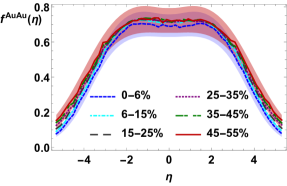
Figure 2: One-particle emission profiles obtained in the wounded quark model from the PHOBOS rapidity spectra for Au-Au collisions at $\sqrt{s_{NN}}=200$ GeV Back et al. (2003) in the indicated centrality classes. The shaded bands give the experimental uncertainties (propagated via the Gaussian method) for the most central and the most peripheral case.

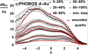
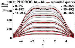
Figure 3: Comparison of the wounded-quark model predictions (lines) with the experimental rapidity spectra (points) for d-Au Back et al. (2005) (a) and Au-Au Back et al. (2003) (b) collisions, with the experimental uncertainties shown as shaded bands. A universal profile discussed in the text is taken for the model calculations in all cases.

If the wounded-quark scaling works, then the profiles obtained with different centrality classes or mass numbers of the colliding nuclei should be universal, depending only on the collision energy. To what extent this is the case, can be assessed from Figs. 1 and 2, which show the one-particle emission profiles that were extracted from experimental data on d-Au and Au-Au collisions from the PHOBOS data Back et al. (2004, 2005, 2003) in the framework of the wounded quark model. To this end, the symmetric (for both reactions) and antisymmetric components (only in the case of the d-Au collisions) were obtained from the experimental data on rapidity spectra by means of Eq. (4), where the valence quark multiplicities $\langle N_{\pm}\rangle$ were obtained from GLISSANDO Broniowski et al. (2009); Rybczyński et al. (2014), a Monte-Carlo simulator of the Glauber model.

Figure 1 shows the results for the one-particle-emission profiles $f^{\rm dAu}(\eta)$ extracted from the PHOBOS data Back et al. (2004, 2005) for d-Au collisions, together with their symmetric and antisymmetric components. In general, the curves for various centrality classes, considering the propagated experimental errors, can be viewed as coinciding. The apparent exception to this behavior is seen in the symmetric part of the profile for the peripheral centrality $60\%-80\%$, which is significantly larger for $|\eta|<3$, cf. Fig. 1(b). We note that for d-Au collisions this peripheral class corresponds to $\langle N_{+}\rangle$ in the range from six to eight sources, which are tiny values, where the model admittedly does not work. It can thus confirm the findings of Barej et al. (2018) that the assumption of universality of the one-particle emission profiles works reasonably well for the central to mid-peripheral d-Au collisions, whereas it starts to differ for more peripheral centrality classes.

Figure 2 presents our results for the one-particle emission profiles $f^{\rm AuAu}(\eta)$ extracted from the PHOBOS data Back et al. (2003) for Au-Au collisions. As already mentioned, in this case only the symmetric parts of the emission profiles can be obtained. It can be seen that the results for $f^{\rm AuAu}(\eta)$ in various centrality classes agree remarkably well with one another. They also approximately agree with the symmetric profiles for d-Au collisions of Fig. 1(b).

Finally, we test if our method reproduces the PHOBOS charged particle rapidity spectra for combined d-Au and Au-Au collisions. To this end we take a single “universal” $f(\eta)$, consisting of an antisymmetric part extracted from the minimum-bias d-Au spectra and a symmetric part taken as the average of the different one-particle emission profiles of Au-Au collisions shown in Fig. 2. The charged particle rapidity spectra $dN_{\rm ch}/d\eta$ were calculated by means of Eq. (2) with this universal $f(\eta)$, where again the numbers $\langle N_{A}\rangle$ and $\langle N_{B}\rangle$ were generated with GLISSANDO. Figure 3 shows the resulting one-particle-emission spectra for d-Au and Au-Au collisions obtained that way, together with the corresponding experimental data from PHOBOS Back et al. (2004, 2005, 2003): As expected from Fig. 2, the rapidity spectra for the Au-Au collisions, which are almost symmetric, are very well reproduced by the chosen $f(\eta)$. Also the rapidity spectra for the d-Au collisions, which largely depend on both the symmetric and antisymmetric contribution to $f(\eta)$, are qualitatively well reproduced for $|\eta|<4$, except for the above-discussed case of the peripheral collisions.

Therefore, we conclude that the wounded quark model with the universal profile function $f(\eta)$ reproduces the experimental rapidity spectra at $\sqrt{s_{NN}}=200$ GeV in a way satisfactory for our exploratory study. In the following analysis of the rapidity fluctuations, we use the $f(\eta)$ obtained here to constrain the string end-point distributions.

III Generic string model

In this section we describe a model of generic production from a single string formed in the early phase of the collision process. Suppose the string is pulled by two end-points placed at spatial rapidities $y_{1}$ and $y_{2}$, whose locations are generated according to a probability distribution $g(y_{1},y_{2})$ (if the end-points are generated in an uncorrelated manner, then $g(y_{1},y_{2})=g_{1}(y_{1})g_{2}(y_{2})$, as will be assumed shortly). The emission of a particle with rapidity $\eta$ from the string fragmentation process is assumed to be uniformly distributed along the string, i.e., it is equal to

$$\!\!\!\!\!s(\eta;y_{1},y_{2})=\omega\left[\theta(y_{1}<\eta<y_{2})+\theta(y_{2}<\eta<y_{1})\right],$$ (5)

where $\omega$ is a dimensionless constant determining the production strength and $\theta(c)$ imposes the condition $c$. Note that we include the cases of $y_{2}>y_{1}$ and $y_{1}>y_{2}$, which may seem redundant but which is needed, for instance, when the two end-points correspond to different partons in a given model.

Let us introduce the short-hand notation

$$\int_{\cal Y}dy_{1}dy_{2}\,g(y_{1},y_{2})X=\langle X\rangle_{\cal Y},$$ (6)

with ${\cal Y}$ denoting the two-dimensional range of integration, depending on the kinematic constraints and/or detector coverage, and $X$ meaning any expression. The single-particle density for production from a string upon averaging over the fluctuation of the end-points is therefore

$$f(\eta)=\langle s(\eta;y_{1},y_{2})\rangle_{\cal Y},$$ (7)

Analogously, for the $n$-particle production ($n\geq 2$) from a single string we have

$$f_{n}(\eta_{1},\dots,\eta_{n})=\langle s(\eta_{1};y_{1},y_{2})\dots s(\eta_{n};y_{1},y_{2})\rangle_{\cal Y},$$ (8)

where we have assumed independent production of the $n$ particles.

In case the string ends are generated independently of each other, one has

$$\langle X\rangle_{\cal Y}=\int dy_{1}dy_{2}g_{1}(y_{1})g_{2}(y_{2})X\,,$$ (9)

where the limits of integration in $y_{i}$ are formally from $-\infty$ to $\infty$, with the support taken care of by the forms of $g_{i}(y_{i})$. Then we readily find that the one-body emission profile is

$$f(\eta) = \omega\left\{G_{1}(\eta)[1-G_{2}(\eta)]+G_{2}(\eta)[1-G_{1}(\eta)]\right\}$$ (10)

$$= \omega\left\{\tfrac{1}{2}-2[G_{1}(\eta)-\tfrac{1}{2}][G_{2}(\eta)-\tfrac{1}{2}]\right\},$$

where the appropriate cumulative distribution functions (CDFs) are defined as

$$G_{i}(y)=\int_{-\infty}^{y}dy^{\prime}\,g_{i}(y^{\prime}).$$ (11)

The profile $f(\eta)$ acquires a specific value at the arguments $\eta_{1}$ and $\eta_{2}$ where the CDFs reach $\tfrac{1}{2}$, i.e.,

$$\eta_{1}^{(0)}\;:\;G_{1}(\eta_{1}^{(0)})=\tfrac{1}{2},$$

$$\eta_{2}^{(0)}\;:\;G_{2}(\eta_{2}^{(0)})=\tfrac{1}{2}.$$ (12)

Then from Eq. (10) we obtain

$$\omega=2f(\eta_{1}^{(0)})=2f(\eta_{2}^{(0)}).$$ (13)

This equation provides a special meaning to the constant $\omega$. Furthermore, since $0\leq G_{1,2}(\eta)\leq 1$, Eq. (10) yields the limit

$$0\leq f(\eta)\leq\omega.$$ (14)

The above features will be explored shortly in a qualitative discussion.

Similarly, for the $n$-particle distributions with $n\geq 2$ we have

$$f_{n}(\eta_{1},\dots,\eta_{n})=\omega^{n}\left\{\right.$$ (15)

$$~{}~{}G_{1}({\rm min}(\eta_{1},\dots,\eta_{n}))[1-G_{2}({\rm max}(\eta_{1},\dots,\eta_{n}))]+$$

$$\left.~{}~{}G_{2}({\rm min}(\eta_{1},\dots,\eta_{n}))[1-G_{1}({\rm max}(\eta_{1},\dots,\eta_{n}))]\right\}.$$

We thus see that in the model with two end-points fluctuating (the relevant assumptions are the uniform string fragmentation (5) and the independence of the two end-point locations) all the information carried by the $n$-particle densities produced from a single string is encoded solely in the cumulative distributions functions $G_{1}$ and $G_{2}$. It is obvious, however, that $G_{1}$ and $G_{2}$ cannot be separately determined from the one-body distributions in an unambiguous manner, hence a large degree of freedom is still left in the model after fixing the rapidity spectra. Yet, the one body distribution provides, via Eq. (10), an important constraint. Our method of matching $G_{1}$ and $G_{2}$ to the one-body function $f(\eta)$ is explained in detail in Appendix A. As we stress, there is no uniqueness in the procedure, but there is a systematic way of approaching the problem, allowing one to explore the range of possibilities.

We denote the position of the maximum of $f(\eta)$ as $\eta_{\rm max}$.

We consider three cases:

1. The distributions of both end-points are equal, $g_{1}(\eta)=g_{2}(\eta)$, Eq. (33). In this case $\omega=2f(\eta_{\rm max})$, with $\eta_{\rm max}=\eta_{1}^{(0)}=\eta_{2}^{(0)}$.

2. The supports of distributions $g_{1}(\eta)$ and $g_{2}(\eta)$ do not overlap, Eq. (LABEL:eq:case2). In this case $\omega=f(\eta_{\rm max})$ and $\eta_{2}^{(0)}<\eta_{\rm max}<\eta_{1}^{(0)}$.

3. The form of $g_{1}(\eta)$ is motivated by parton distribution functions (PDFs) of valence quarks, Eq. (44), and $g_{2}(\eta)$ is adjusted according to Eq. (35).

Cases i) and ii) are in a sense most different, showing the span of possibilities formally allowed, whereas case iii) is intermediate. For case iii) we use the parametrization of the valence quark PDF given by Eq. (44) with parameters $\alpha=-0.5$ and $\beta=3$, which are typical values at low scales. We have found that using other reasonable parametrizations has very small influence on our results, with case iii) always remaining close to case i).

We stress that all the considered cases reproduce, by construction, the one-body emission profiles $f(\eta)$.

We end this section with remarks concerning the model with one end of the string fixed and the other one fluctuating, explored in Broniowski and Bożek (2016). This simplified version can be obtained as a special limit from Eqs. (10,15) by choosing $g_{1}(\eta)=\delta(\eta-y_{\rm max})$, which is equivalent of taking, correspondingly, $G_{1}=0$ for $\eta<y_{\rm max}$, i.e.,

$$f(\eta) = \omega G_{2}(\eta),$$ (16)

$$f_{n}(\eta_{1},\dots,\eta_{n}) = \omega^{n}G_{2}({\rm min}(\eta_{1},\dots,\eta_{n})).$$

We note immediately that this model cannot reproduce $f(\eta)$ for $\eta>\eta_{\rm max}$, as $G_{2}(\eta)$ cannot decrease. Thus the model is limited to $\eta\leq\eta_{\rm max}$, which, however, is not a problem if we are only interested in the mid-rapidity region.

Moreover, in this region the single-end fluctuating model corresponds precisely to case ii) of the two-end fluctuations. This is obvious from the following argumentation: When the right end of the string is fluctuating outside of the acceptance region, it is irrelevant if it fluctuates or if it is fixed, as in both cases we only observe the production from the part of the string falling into the acceptance range. In that situation (or more precisely for $\eta\leq\eta_{\rm max}$) Eqs. (10,15) reduce to Eqs. (16). Hence, the single end-point fluctuation model of Broniowski and Bożek (2016) corresponds to the present case ii) at $\eta\leq\eta_{\rm max}$, and is not applicable for $\eta>\eta_{\rm max}$.

IV End-point distributions

We now come to the discussion of the end-point distributions subjected to the requirement that the one-body emission profiles are reproduced.

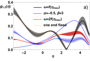
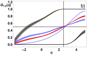
Figure 4: Distribution functions $g_{1}$ and $g_{2}$ (a) and cumulative distribution functions $G_{1}$ and $G_{2}$ (b) of the string end-points for the cases of i) $\omega=2f(\eta_{\rm max})$, ii) $\omega=f(\eta_{\rm max})$, and iii) $\alpha=-0.5,$ $\beta=3$, as indicated in the legend. The light dot-dashed line corresponds to the model with one end-point fixed and the other one fluctuating Broniowski and Bożek (2016), which overlaps with case ii) for $\eta\leq\eta_{\rm max}$. The vertical line in panel (b) indicates $\eta=\eta_{\rm max}$. See the text for further details.

Figure 4a) shows the distributions of the string end-points, $g_{1}$ and $g_{2}$, for the three cases, and Fig. 4b) the corresponding CDFs, $G_{1}$ and $G_{2}$. The shaded bands give an estimate of the errors due to the experimental uncertainty $\Delta f$ for the one-particle emission profile $f$. In the case of Fig. 4b), the upper limit of the shaded bands corresponds to the values of $G_{1,2}$ that are matched to the one-body profile $f+\Delta f$, whereas the lower limits are matched to $f-\Delta f$. For these upper and lower limits of $G_{1,2}$, the derivatives in $\eta$ yield the upper and lower limits of the shaded bands for $g_{1}$ and $g_{2}$ depicted in Fig. 4a). For case iii) a shaded band is given only for $g_{2}$ ($G_{2}$). This is because by construction $g_{1}$ ($G_{1}$) coming from PDFs are assumed to be accurate and all uncertainty is therefore attributed to $g_{2}$ ($G_{2}$).

In case i) $g_{1}(\eta)=g_{2}(\eta)$, hence the distributions are indicated with a single curve (solid line) in Figs. 4a) and b). We note that the distribution of $g_{1}(\eta)$ peaks at forward rapidity (the Au side), as expected from the shape of the one-body profile $f(\eta)$ in Fig. 1. The CDF crosses the value $1/2$ at $\eta_{1}^{(0)}=\eta_{2}^{(0)}=\eta_{\rm max}\simeq 2.5$, which coincides with the maximum of $f(\eta)$.

In case ii) (dashed lines in Fig. 4) the supports for $g_{1}$ and $g_{2}$ are disjoint. In Fig. 4a) the left part of the curve, up to the point $\eta_{\rm max}\simeq 2.5$ (indicated with a vertical line), corresponds to $g_{2}$, and the right part to $g_{1}$. Hence, the string end-points always follow the ordering $y_{1}\geq y_{2}$, which does not hold in the other cases. Figure 4b) shows the corresponding CDFs, with $G_{1}=0$ left from $\eta_{\rm max}$, and $G_{2}=1$ right from $\eta_{\rm max}$. In Appendix A we show that $G_{1}$ and $G_{2}$ from case ii) are the lower and upper limits for any CDFs in the considered problem. Indeed, the CDFs from the other two cases fall in between these limiting curves.

Case iii), based on a valence quark PDF for $g_{1}$, represents an intermediate class of distributions falling between cases i) and ii). The curves corresponding to the valence quark are dotted and with no error bands. The distribution $g_{1}$ (valence quark) is peaked in the forward direction, as expected. We note that $y_{1}>y_{2}$ is favored, although $y_{2}<y_{1}$ is also possible. With the parametrization we used of the valence quark distribution, the CDFs in case iii) are not far from case i). We have checked that this feature holds also for other reasonable parametrizations of the valence quark PDF.

We underline again that all the cases of Fig. 4, which exhibit radically different end-point distributions, reproduce by construction the one-body emission profile $f(\eta)$.

V Correlations from a single string

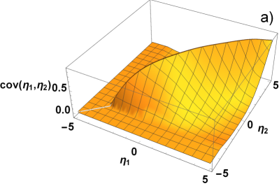
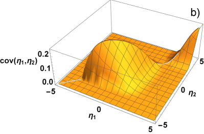
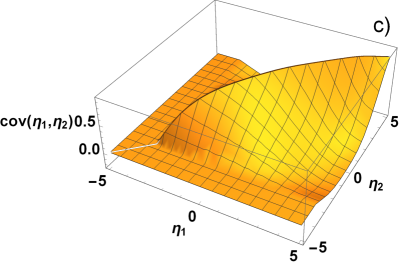
Figure 5: Covariance for the emission from a single string for cases i) (a), ii) (b) and iii) (c).

As we show in this section, the two-particle correlation is sensitive to the particular form of the distributions and differs between cases i), ii), and iii). A convenient quantity is the covariance of the two-particle emission from a single string, defined as

$${\rm cov}(\eta_{1},\eta_{2})={f_{2}(\eta_{1},\eta_{2})}-{f(\eta_{1})}{f(\eta_{2})},$$ (17)

where $f_{2}$ is given by Eq. (15). Explicitly,

$${\rm cov}(\eta_{1},\eta_{2})=\omega^{2}\big{\{}G_{1}({\rm min}(\eta_{1},\eta_{2}))[1-G_{2}({\rm max}(\eta_{1},\eta_{2}))]$$

$$~{}~{}~{}+G_{2}({\rm min}(\eta_{1},\eta_{2}))[1-G_{1}({\rm max}(\eta_{1},\eta_{2}))]$$

$$~{}~{}~{}-\left(G_{1}(\eta_{1})[1-G_{2}(\eta_{1})]+G_{2}(\eta_{1})[1-G_{1}(\eta_{1})]\right)$$

$$~{}~{}~{}\times\left(G_{1}(\eta_{2})[1-G_{2}(\eta_{2})]+G_{2}(\eta_{2})[1-G_{1}(\eta_{2})]\right)\big{\}}.$$ (18)

A simplification occurs along the diagonal $\eta_{1}=\eta_{2}=\eta$, where

$${\rm cov}(\eta,\eta) = \omega^{2}\big{\{}\tfrac{1}{4}\!-\!4[G_{1}(\eta)-\tfrac{1}{2}]^{2}[G_{2}(\eta)-\tfrac{1}{2}]^{2}\big{\}}$$ (19)

$$= f(\eta)[\omega-f(\eta)].$$

Also, the leading expansion at the diagonal in the anti-diagonal direction, with $\eta_{1}=\eta+\delta$ and $\eta_{2}=\eta-\delta$, yields a very simple formula,

$${\rm cov}(\eta\!+\!\delta,\eta\!-\!\delta)={\rm cov}(\eta,\eta)-\omega^{2}[g_{1}(\eta)\!+\!g_{2}(\eta)]|\delta|+{\cal O}(\delta^{2}).$$

(20)

Figure 5 shows the resulting distributions for ${\rm cov}(\eta_{1},\eta_{2})$ for the three considered cases. One observes vivid qualitative differences between the covariances in cases i) and ii), cf. Figs. 5a) and b). Whereas in case i) the covariance exhibits a monotonously increasing ridge along the $\eta_{1}=\eta_{2}$ direction, the covariance in case ii) shows a double peak structure, with a zero at $\eta=\eta_{\rm max}\simeq 2.5$, which corresponds to the zero of $g_{1}$ and $g_{2}$ in Fig. 4a). At this point $G_{1}(\eta)=0$ and $G_{2}(\eta)=1$, which upon substitution to Eq. (18) yields zero. Another difference is in magnitude of the covariance, which in case i) is significantly larger than in case ii).

The covariance in case iii) is very close to case i) (cf. Figs. 5a) and c)). Some small difference can be seen where $\eta_{1}$ is small(large), but $\eta_{2}$ large(small), where in case iii) the covariance noticeably drops to negative values.

We also note that in all cases the values on the diagonal is obeying Eq. (19). The fall-off from the diagonal in the anti-diagonal direction is given by the second term in Eq. (20). We note that the slope is proportional to $4f(\eta_{1,2}^{(0)})[g_{1}(\eta)+g_{2}(\eta)]$, hence two models which have similar values of $\eta_{1,2}^{(0)}$ and close sums of the two end-point distributions, $g_{1}(\eta)+g_{2}(\eta)$, will have similar covariances in the vicinity of the diagonal. Both conditions are satisfied between models i) and iii). In particular, we can see that the sum $g_{1}(\eta)+g_{2}(\eta)$ for model iii) in Fig. 4a) (dotted lines) is close to twice $g_{1,2}(\eta)$ for model i) (solid line).

Thus the reason for the similarity of correlations in cases (i) and (iii) may be traced back to Eq. (20), which shows that this is the average of $g_{1}(\eta)$ and $g_{2}(\eta)$, which controls the fall-off of the correlation from the diagonal. These averages happen to be very similar when we use any reasonable parametrization of the parton distribution function giving the PDF of one end-point distribution, and the fluctuations the other end-point are adjusted to match the profile function $f(\eta)$, as explained in Sec. IV.

VI Correlations from multiple strings

As already discussed in the introduction, in our approach the strings “belong” to the valence quarks either from nucleus A or from nucleus B. With the underlying assumptions of independent wounded sources, the expressions for the $n$-body distributions account for the combinatorics in a simple manner, with the particles at rapidities $\eta_{i}$ being products from a string belonging to $A$ or to $B$. For the one-body density in A-B collisions one finds

$${f_{AB}(\eta)}=\langle N_{A}\rangle{f_{A}(\eta)}+\langle N_{B}\rangle{f_{B}(\eta)},$$ (21)

where $\langle N_{A}\rangle$ and $\langle N_{B}\rangle$ are the event-by-event average numbers of wounded sources in nuclei A and B, respectively, and $f_{A,B}(\eta)=f(\pm\eta)$ denote the profiles for the emission from a single string, as given by Eq. (7), associated with sources from nuclei $A$ or $B$. We work in the nucleon-nucleon center-of-mass (CM) frame, hence $f_{A}(\eta)=f_{B}(-\eta)$.

Analogously, one can define the two-body distribution for emission from a single string in nuclei $A$ and $B$ as $f_{A,B}(\eta_{1},\eta_{2})=f_{2}(\pm\eta_{1},\pm\eta_{2})$, and the corresponding covariances as ${\rm cov}_{A,B}(\eta_{1},\eta_{2})={\rm cov}(\pm\eta_{1},\pm\eta_{2})$. Then, one readily obtains the covariance for the production in A-B collisions (see Appendix C) in the form

$${\rm cov}_{AB}(\eta_{1},\eta_{2})\equiv f_{AB}(\eta_{1},\eta_{2})-f_{AB}(\eta_{1})f_{AB}(\eta_{2})$$

$$= \langle N_{A}\rangle{\rm cov}_{A}(\eta_{1},\eta_{2})+\langle N_{B}\rangle{\rm cov}_{B}(\eta_{1},\eta_{2})$$

$$+ {\rm var}(N_{A}){f_{A}(\eta_{1})}{f_{A}(\eta_{2})}+{\rm var}(N_{B}){f_{B}(\eta_{1})}{f_{B}(\eta_{2})}$$

$$+ {\rm cov}(N_{A},N_{B})\left[{f_{A}(\eta_{1})}{f_{B}(\eta_{2})}+{f_{B}(\eta_{1})}{f_{A}(\eta_{2})}\right].$$

In the special case of symmetric collisions Eq. (VI) simplifies into

$${\rm cov}_{AB}(\eta_{1},\eta_{2})=\langle N_{A}\rangle{\rm cov}_{A}(\eta_{1},\eta_{2})+\langle N_{B}\rangle{\rm cov}_{B}(\eta_{1},\eta_{2})$$

$$+{\rm var}(N_{+}){f_{s}(\eta_{1})}{f_{s}(\eta_{2})}+{\rm var}(N_{-}){f_{a}(\eta_{1})}{f_{a}(\eta_{2})},$$ (23)

where $N_{-}=N_{A}-N_{B}$. The moments of $N_{A}$ and $N_{B}$ evaluated with GLISSANDO are listed in Appendix D.

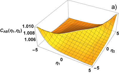
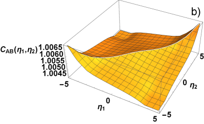
Figure 6: Correlations $C_{AB}(\eta_{1},\eta_{2})$ for the $6\%$ most central Au-Au collisions for model cases i) (a) and ii) (b), as well as $C^{\ast}_{AB}(\eta_{1},\eta_{2})$ for case i) (c).

We also introduce the customary correlation $C$ defined as

$$C_{AB}(\eta_{1},\eta_{2})=1+\frac{{\rm cov}_{AB}(\eta_{1},\eta_{2})}{f_{AB}(\eta_{1})f_{AB}(\eta_{2})},$$ (24)

which is a convenient measure due to its intensive property. For symmetric collisions Eq. (24) becomes

$$C_{AB}(\eta_{1},\eta_{2})=1+\frac{{\rm cov}_{AB}(\eta_{1},\eta_{2})}{\langle N_{+}\rangle^{2}f_{s}(\eta_{1})f_{s}(\eta_{2})},$$ (25)

To separate the contribution from the string end-point fluctuations, we also define

$$C^{\ast}_{AB}(\eta_{1},\eta_{2})=\frac{\langle N_{A}\rangle{\rm cov}_{A}(\eta_{1},\eta_{2})+\langle N_{B}\rangle{\rm cov}_{B}(\eta_{1},\eta_{2})}{f_{AB}(\eta_{1})f_{AB}(\eta_{2})}.$$

(26)

We note that Eq. (VI) or (23) contain terms with two classes of fluctuations: those stemming from single string end-point fluctuations, containing ${\rm cov}_{i}(\eta_{1},\eta_{2})$, which were the object of study in the previous section, and the remaining terms Bzdak and Teaney (2013) with moments of fluctuations of the numbers of wounded quarks, $N_{A}$ and $N_{B}$. Therefore the correlation function $C(\eta_{1},\eta_{2})$ contains a mixture of both effects. In principle, one could separate these effects via the technique of partial covariance (see, e.g., Cramer (1946); Krzanowski (2000)), which effectively imposes constraints on a multivariate sample. The details of such an analysis, which leads to very simple and practical expressions, were presented in Olszewski and Broniowski (2017).

In the present case, however, such an analysis is not necessary if we have in mind the standard $a_{nm}$ coefficients discussed in Sec. VII. As is clear from Eq. (25), the term ${\rm var}(N_{+}){f_{s}(\eta_{1})}{f_{s}(\eta_{2})}$ in Eq. (23) brings in a constant ${\rm var}(N_{+})/\langle N_{+}\rangle^{2}$ into $C(\eta_{1},\eta_{2})$. Therefore it only changes its baseline and does not affect the $a_{nm}$ coefficients (for $n,m\geq 0$). As we shall shortly see, the string end-point fluctuations given by the term with $\langle N_{A}\rangle{\rm cov}_{A}(\eta_{1},\eta_{2})+\langle N_{B}\rangle{\rm cov}_{B}(\eta_{1},\eta_{2})$ are largely dominant over the Bzdak-Teaney Bzdak and Teaney (2013) term, ${\rm var}(N_{-}){f_{a}(\eta_{1})}{f_{a}(\eta_{2})}$, with the later entering at a level of 10-20% in $a_{11}$ (cf. Sec. VII). Hence one may simply take the view that measuring the $a_{nm}$ coefficients associated with $C(\eta_{1},\eta_{2})$ essentially provides information on the string end-point fluctuations, with only a small contamination by the fluctuation of the number of sources.

Panels a) and b) of Fig. 6 show our results for $C_{AB}(\eta_{1},\eta_{2})$ of the $6\%$ most central Au-Au collisions at $\sqrt{s_{NN}}=200$ GeV in cases i) and ii) of our model. The correlations exhibit a ridge structure along the $\eta_{1}=\eta_{2}$ direction, which simply reflects the presence of the ridges in the single-string fluctuations displayed in Fig. 5. The correlation in case iii) is very close to case i), simply reflecting the behavior of Fig. 5, hence we do not include it in the plot.

Panel c) shows the correlation stemming from the fluctuation of the string end-point, $C^{\ast}_{AB}(\eta_{1},\eta_{2})$ of Eq. (26). We note that, apart for an overall shift by a constant, it is very similar to the correlation $C_{AB}(\eta_{1},\eta_{2})$ of Eq. (24), which indicates an important feature shown by our study: The shape of the correlation function $C(\eta_{1},\eta_{2})$ is largely dominated by the string end-point fluctuations, whereas the effects of the fluctuations of the number of sources are small.

VII $a_{nm}$ coefficients

​ ​

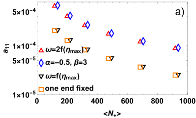
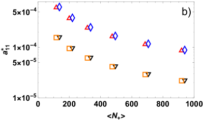
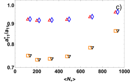
Figure 7: $a_{11}$ (a) and $a^{\ast}_{11}$ (b) for Au-Au collisions at $\sqrt{s_{\rm NN}}=200$ GeV as a function of $\langle N_{+}\rangle$ (the selected values for $\langle N_{+}\rangle$ correspond to the $6$ centrality classes $0-6\%$, $6-15\%$, $15-25\%$, $25-35\%$, $35-45\%$, and $45-55\%$) in cases i) with $\omega=2f(\eta_{\rm max})$, ii) with $\omega=f(\eta_{\rm max})$, iii) with $\alpha=-0.5,\,\beta=3$, together with the model of Broniowski and Bożek (2016) with one end point fixed, as indicated in the legend. Panel c) displays the ratio $a^{\ast}_{11}/a_{11}$. To enhance visibility, the markers for the overlapping cases are slightly shifted to the left or right along the abscissa.

For a given correlation function $C(\eta_{1},\eta_{2})$, the $a_{nm}$ coefficients are defined as Bzdak and Teaney (2013); Aad et al. (2015a, b)

$$a_{nm} = \int_{-Y}^{Y}\frac{d\eta_{1}}{Y}\int_{-Y}^{Y}\frac{d\eta_{2}}{Y}\frac{1}{\mathcal{N}_{C}}C(\eta_{1},\eta_{2})T_{n}\left(\frac{\eta_{1}}{Y}\right)T_{m}\left(\frac{\eta_{2}}{Y}\right),$$

with the normalization constant

$$\mathcal{N}_{C}=\int_{-Y}^{Y}\frac{d\eta_{1}}{Y}\int_{-Y}^{Y}\frac{d\eta_{2}}{Y}C(\eta_{1},\eta_{2}),$$ (28)

where $[-Y,Y]$ is the covered pseudorapidity range. Having in mind the typical pseudorapidity acceptance at RHIC, we use $Y=1$. The functions $T_{n}(x)$ form a set of orthonormal polynomials. The choice used in Aad et al. (2015a, b); Jia et al. (2016) is

$$T_{n}(x)=\sqrt{n+1/2}P_{n}(x),$$ (29)

where $P_{n}(x)$ are the Legendre polynomials.

Analogously, we define

$$a_{nm}^{\ast} = \int_{-Y}^{Y}\frac{d\eta_{1}}{Y}\int_{-Y}^{Y}\frac{d\eta_{2}}{Y}\frac{1}{\mathcal{N}_{C}}C^{\ast}(\eta_{1},\eta_{2})T_{n}\left(\frac{\eta_{1}}{Y}\right)T_{m}\left(\frac{\eta_{2}}{Y}\right),$$

which focuses on the fluctuations of the strings (note that the normalization constant ${\mathcal{N}_{C}}$ is evaluated with $C(\eta_{1},\eta_{2})$ as in Eq. (LABEL:eq:anmC)).

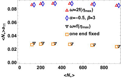
Figure 8: The product of $a_{11}$ and $\langle N_{+}\rangle$, showing the scaling discussed in the text.

Figure 7 shows our results for $a_{11}$ (panel a) and $a^{\ast}_{11}$ (panel b) obtained for Au-Au collisions at $\sqrt{s_{\rm NN}}=200$ GeV and plotted as functions of the average number of wounded quarks $\langle N_{+}\rangle$ in selected centrality classes. We note that the results for model cases i) and iii) are essentially identical, reflecting the feature seen already in Fig. (6). The result for case ii) is about a factor of 3 smaller. In this and following figures we also indicate the results for the model with single end-point fluctuations, which is identical to case ii) in the considered acceptance region.

In view of the discussion of Sec. IV, cases i) and ii) in Fig. 7 represent the upper and lower bounds for the admissible values of the $a_{11}$ coefficients. This is an important result, as it provides the possible range for this quantity in approaches sharing the features of our model.

In panel c) of Fig. 7 we present the ratio $a^{\ast}_{11}/a_{11}$, which shows the announced dominance of the string end-point fluctuations over the fluctuation of the numbers of sources. In model cases i) and iii) the former account for 90% of the effects, whereas in case ii) they account for 75-85%.

From Eqs. (23,26) it is clear that $a^{\ast}_{11}$ scales as $1/\langle N_{+}\rangle$. For $a_{11}$ there is a small departure of a relative order ${\rm var}(N_{-})/\langle N_{+}\rangle$. Numerically, for models i) and ii) $a^{\ast}_{11}\sim 0.08/\langle N_{+}\rangle$, whereas the leading term of expansion (20) yields a close result $a^{\ast}_{11}\sim 0.1/\langle N_{+}\rangle$. The approximate scaling for $a_{11}$ is exhibited in Fig. 8.

A similar analysis of the $a_{11}$ coefficients for the d-Au collisions yields qualitatively similar results, shown in Fig. 9. Here, the coefficients $a_{11}^{\ast}$ account for more than $90\%$ of the total, hence the dominance of string end-point fluctuations is even more pronounced in d-Au than in Au-Au collisions. For that reason we present only the results for $a_{11}$.

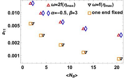
Figure 9: Same as in Fig. 7a) but for d-Au collisions at $\sqrt{s_{\rm NN}}=200$ GeV, plotted as a function of the average number of wounded quarks in Au, $\langle N_{B}\rangle$ (selected values for $\langle N_{B}\rangle$ correspond to centrality classes $0-20\%$, $20-40\%$, $40-60\%$, $60-80\%$).

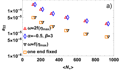
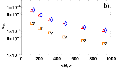
Figure 10: Same as in Fig. 7a) but for $a_{22}$ (a) and $-a_{13}$ (b).

In addition to $a_{11}$ coefficients, one may study the higher-order $a_{nm}$ coefficients. We give our results for $a_{13}$ and $a_{22}$ from Au-Au collisions in Fig.  10. While these coefficients are considerably suppressed as compared to $a_{11}$, shown in Fig. 10, they exhibit the same qualitative behavior. In particular, they scale almost exactly as $1/\langle N_{+}\rangle$.

Finally, we remark that when the model results are to be compared to experimental values, one needs to relate the space-time rapidity of the initial stage, $\eta_{PS}=\frac{1}{2}\ln[(t+z)/(t-z)]$ (until now denoted as $\eta$ in our considerations), to the momentum pseudorapidity of the measured hadrons, $\eta=\frac{1}{2}\log[(E+p_{z})/(E-p_{z})]$. The experience of hydrodynamic simulations shows a mild longitudinal push, yielding $\eta\simeq 1.25\,\eta_{PS}$. This effect leads to a quenching factor of about 1.5 to be applied to the model $a_{nm}$ coefficients before comparing to the data.

VIII Conclusions

We have analyzed a model where strings are associated with wounded quarks and their end-points fluctuate. We have used the data for the pseudo-rapidity spectra for d-Au and Au-Au collisions from the PHOBOS Collaboration at $\sqrt{s_{NN}}=200$ GeV to impose constraints on the one-body distributions in the model. We have selected a RHIC energy for our study, since the wounded quark model works very well in this case.

We first confirmed the results of Barej et al. (2018) that a thus extracted one-body emission function reproduces reasonably well the experimental rapidity spectra and therefore is universal in the sense that it can be applied to different centrality classes and collision systems for the considered collision energy. Then we showed that there remains a substantial freedom in string end-point distributions $G_{1,2}$, which gives rise to a family of possible solutions. Specifically, we have discussed three cases of solutions: the limiting cases i) and ii) and an intermediate case iii), inspired by the valence quark parton distribution function. We have argued that case ii) is equivalent to the model with single end-point fluctuations of Broniowski and Bożek (2016), if the acceptance window at mid-rapidity is sufficiently narrow.

The analysis was carried out analytically, which has its obvious merits. We obtained formulas for the $n$-body distributions of the produced particles. In the study of the two-body correlations, we have examined the effects from string end-point fluctuations and from the fluctuation of the number of sources. The former largely dominate in the corresponding Legendre coefficients $a_{nm}$.

We have found that the range for fluctuations is limited by two extreme cases. The lower limit, where the domains of the fluctuations of both ends do not overlap, coincides (for sufficiently narrow acceptance windows in pseudorapidity) with the model with single-end fluctuations considered earlier in Broniowski and Bożek (2016). Allowing for both ends to fluctuate increases significantly the fluctuations, raising the $a_{nm}$ coefficients by a factor of $\sim 3$.

A variant of the model where the distribution of one end of the string follows the valence quark PDF, is very close to the case giving maximum correlation (our case i)). Our results, in particular the presented bounds, can serve as a baseline for future data analysis of the forward-backward fluctuations in rapidity at $\sqrt{s_{NN}}=200$ GeV.

Our simple approach, while neglecting many possible effects such as mutual influence of the strings (merging into color ropes, nuclear shadowing), short range correlations of various origin, or assuming strings of only one type, incorporates two basic and generic features: fluctuation of the number of strings and fluctuation of the location of the string end-points. This makes its predictions valuable for understanding the underlying mechanisms. It remains to be seen to what extent our analytic approach can be extended to more general models, in particular going beyond the simple Glauber wounded picture.

Appendix A Matching the cumulative distribution functions to one-body emission profiles

It is convenient to introduce the shifted CDFs

$$H_{i}(\eta)=G_{i}(\eta)-\frac{1}{2},$$ (31)

which grow from the value $-1/2$ up to $1/2$. Then Eq. (10) can be rewritten as

$$H_{1}(\eta)H_{2}(\eta)=\frac{1}{4}-\frac{1}{2\omega}f(\eta).$$ (32)

We shall now consider three specific cases. In the first case, the maximum of $f(\eta)$ is taken to be $\omega/2$, which is the lowest possible value (otherwise it would contradict Eq. (13)). The position of the maximum is at $\eta_{0}=\eta^{(1)}_{0}=\eta^{(2)}_{0}$ (the two zeros of $H_{i}(\eta)$ coincide in this case). Then the solution takes the form

$$H_{1}(\eta) = \sqrt{\frac{1}{4}-\frac{1}{2\omega}f(\eta)}\,{\rm sgn}(\eta-\eta_{0})s(\eta),$$

$$H_{2}(\eta) = \sqrt{\frac{1}{4}-\frac{1}{2\omega}f(\eta)}\,{\rm sgn}(\eta-\eta_{0})/s(\eta),$$ (33)

where ${\rm sgn}$ denotes the sign function, and $s(\eta)$ is an arbitrary function chosen in such a way that the required limiting and monotonicity properties of $H_{i}(\eta)$ are preserved (one possibility, which we use, is $s(\eta)=1$, in which case both distributions are the same).

The second special case is when the maximum of $f(\eta)$ is $\omega$, which is the largest possible value. Then one may choose

$$H_{1}(\eta) = -\frac{1}{2}\theta(\eta_{0}-\eta)+\left[\frac{1}{2}-\frac{1}{\omega}f(\eta)\right]\theta(\eta-\eta_{0}),$$

$$H_{2}(\eta) = -\left[\frac{1}{2}-\frac{1}{\omega}f(\eta)\right]\theta(\eta_{0}-\eta)+\frac{1}{2}\theta(\eta-\eta_{0}).$$

In this case the supports of $g_{1}(\eta)$ and $g_{2}(\eta)$ are disjoint.

We can now easily verify that the formulas (33) and (LABEL:eq:case2) indeed satisfy Eq. (32).

In the intermediate case, when the maximum satisfies $\omega/2<f(\eta)\leq\omega$, one may generically take a “favorite” form of $H_{1}(\eta)$ and then evaluate $H_{2}(\eta)$ from Eq. (32) as

$$H_{2}(\eta)=\frac{\frac{1}{4}-\frac{1}{2\omega}f(\eta)}{H_{1}(\eta)}.$$ (35)

Note that $H_{2}(\eta)$ is well-behaved near $\eta_{1}$, as in its vicinity

$$H_{1}(\eta)=C_{1}^{2}(\eta-\eta_{1})+\dots,$$

$$\frac{f(\eta)}{\omega}=\frac{1}{2}-C_{2}^{2}(\eta-\eta_{1})^{2}+\dots,$$ (36)

where $C_{1}^{2}$ and $C_{2}^{2}$ denote positive constants, hence

$$H_{2}(\eta)=\frac{C_{2}^{2}}{2C_{1}^{2}}(\eta-\eta_{1})+\dots.$$ (37)

One needs to check explicitly if $H_{2}(\eta)$ obtained from Eq. (35) is a growing function, otherwise the initial choice of $H_{1}(\eta)$ is inconsistent.

Since $-\tfrac{1}{2}\leq H_{1}(\eta)\leq\tfrac{1}{2}$, it follows immediately from Eq. (35) that

$$H_{2}(\eta)\geq\frac{1}{2}-\frac{1}{\omega}f(\eta){\rm~{}~{}for~{}}\eta\geq\eta_{0},$$

$$H_{2}(\eta)\leq-\frac{1}{2}-\frac{1}{\omega}f(\eta){\rm~{}~{}for~{}}\eta\leq\eta_{0}$$ (38)

(and similarly for $H_{1}$), hence the expressions (LABEL:eq:case2) provide upper and lower limits for any CDF for the considered problem.

Appendix B PDF-motivated distribution

When the string end-points $y_{1,2}$ are associated with subnucleonic constituents, such as a valence or sea quark, gluon, or diquark, then they carry the fractions $x_{iA}$ or $x_{iB}$ of the longitudinal momenta of the nucleons inside beams $A$ and $B$, respectively. Specifically, if the momentum of the constituent is $k_{iA}$ ($k_{iB}$) and the momentum of the nucleon is $P_{A}$ ($P_{B}$), then from standard kinematic considerations the corresponding rapidity $y_{iA}$ ($y_{iB}$) of the end-point is related to $x_{iA}$ ($x_{iB}$) with the exact formula

$$x_{iA}\equiv\frac{k_{iA}^{+}}{P_{A}^{+}}=\frac{m_{Ti}}{M}e^{y_{iA}-y_{b}},$$

$$x_{iB}\equiv\frac{k_{iB}^{+}}{P_{B}^{+}}=\frac{m_{Ti}}{M}e^{-y_{iB}-y_{b}},$$ (39)

where $m_{T\,i}=\sqrt{m_{i}^{2}+k_{T\,i}^{2}}$ is the transverse mass of the constituent, $M$ is the mass of the nucleon, and $y_{b}$ is the rapidity of beam $A$ (in the assumed CM frame of the nucleon-nucleon collision, $-y_{b}$ is the rapidity of beam $B$).

The distributions of the locations of the string end-points are then defined via partonic distributions $p_{i}(x)$ as follows:

$$g_{i}(y_{iQ})dy_{iQ}=p_{i}(x_{iQ}(y_{iQ}))dx_{iQ},$$ (40)

with $Q=A,B$, or for the corresponding CDFs

$$G_{i}(y_{iQ})=P_{i}(x_{iQ}(y_{iQ})),.$$ (41)

Since $x_{i\,Q}\in[0,1]$, the limits for the rapidities of the end points are $y_{iA}\in(-\infty,y_{i\uparrow}]$ and $y_{iB}\in[-y_{i\uparrow},\infty)$, where

$$y_{i\uparrow}=y_{b}+\log\left(\frac{M}{m_{Ti}}\right).$$ (42)

In the CM reference frame of the nucleon-nucleon collision, the rapidity of the beam is

$$y_{b}=\log\frac{\sqrt{s/4}+\sqrt{s/4-M^{2}}}{\sqrt{s/4}-\sqrt{s/4-M^{2}}}\simeq\log\frac{\sqrt{s}}{M},$$ (43)

therefore at $\sqrt{s}\gg M$ we have to a good approximation $y_{i\,\uparrow}\simeq\log\frac{\sqrt{s}}{m_{Ti}}$.

In the example used in this paper, a simple parametrization of the parton distribution functions (PDF) is used. Following many phenomenological studies, we take

$$p(x)=Ax^{\alpha}(1-x)^{\beta},$$ (44)

with the corresponding CDF

$$P(x)=\frac{B(x,1+\alpha,1+\beta)}{B(1,1+\alpha,1+\beta)},$$ (45)

where $B(z,a,b)$ denotes the incomplete Euler Beta function.

Table 1: First few moments of the wounded quark numbers in Au-Au collisions at $\sqrt{s_{NN}}=200$ GeV as obtained from GLISSANDO simulations. The chosen centrality classes correspond to those in the PHOBOS experiment.

Centrality [%]	$\langle{N_{+}}\rangle$	${\rm var}(N_{+})$	${\rm var}(N_{-})$
0-6	929	4280	502
6-15	696	4649	653
15-25	484	2972	563
25-35	326	1472	399
35-45	210	811	262
45-55	126	396	144

Table 2: Same as in Table 1 but for d-Au collisions at $\sqrt{s_{NN}}=200$ GeV. Here $N_{A}$ and $N_{B}$ denote the number of wounded quarks in d and Au, respectively.

Centrality [%]	$\langle{N_{A}}\rangle$	$\langle{N_{B}}\rangle$	${\rm var}(N_{A})$	${\rm var}(N_{B})$	${\rm cov}(N_{A},N_{B})$
0-20	5.9	20.6	0.1	14.8	0.1
20-40	5.3	13.1	0.8	2.8	-0.3
40-60	4.1	8.3	1.0	2.7	-0.4
60-80	2.8	4.1	0.6	1.4	0.0
80-100	1.6	1.9	0.3	0.3	-0.1

Appendix C $2$-body density

When we consider the two-body density of particles produced from multiple strings formed in A-B collisions, there are several combinatorial cases which may occur: the two particles may originate from the same string associated with A, from different strings associated with A, from the same string associated with B, from different strings associated with B, and finally one particle is emitted from a string associated with A and the other from as string associated with B. Thus, the two-body density averaged over events in A-B collisions takes the form

$$f_{AB}(\eta_{1},\eta_{2})=$$

$$\langle N_{A}\rangle f_{A}(\eta_{1},\eta_{2})+\langle N_{A}(N_{A}-1)\rangle f_{A}(\eta_{1})f_{A}(\eta_{2})$$

$$+\langle N_{B}\rangle f_{B}(\eta_{1},\eta_{2})+\langle N_{B}(N_{B}-1)\rangle f_{B}(\eta_{1})f_{B}(\eta_{2})$$

$$+\langle N_{A}N_{B}\rangle(f_{A}(\eta_{1})f_{B}(\eta_{2})+f_{B}(\eta_{1})f_{A}(\eta_{2}))\,,$$ (46)

We define the covariances in the usual way,

$${\rm cov}_{A}(\eta_{1},\eta_{2}) =f_{A}(\eta_{1},\eta_{2})-f_{A}(\eta_{1})f_{A}(\eta_{2})\,,$$

$${\rm cov}_{B}(\eta_{1},\eta_{2}) =f_{B}(\eta_{1},\eta_{2})-f_{B}(\eta_{1})f_{B}(\eta_{2}).$$ (47)

Then

$$f_{AB}(\eta_{1},\eta_{2})=$$

$$\langle N_{A}\rangle{\rm cov}_{A}(\eta_{1},\eta_{2})+\langle N_{A}^{2}\rangle{f_{A}(\eta_{1})}{f_{A}(\eta_{2})}$$

$$+\langle N_{B}\rangle{\rm cov}_{B}(\eta_{1},\eta_{2})+\langle N_{B}^{2}\rangle{f_{B}(\eta_{1})}{f_{B}(\eta_{2})}$$

$$+\langle N_{A}N_{B}\rangle({f_{A}(\eta_{1})}{f_{B}(\eta_{2})}+{f_{B}(\eta_{1})}{f_{A}(\eta_{2})}),$$ (48)

and Eq. (VI) follows.

Appendix D Moments of the wounded quark distributions

The lowest moments of the wounded quark distributions obtained form GLISSANDO Broniowski et al. (2009); Rybczyński et al. (2014) and used in our analysis are collected in Tables 1 and 2.

References

- Broniowski and Bożek (2016) W. Broniowski and P. Bożek, Phys. Rev. C93, 064910 (2016), arXiv:1512.01945 [nucl-th] .
- Białas (2008) A. Białas, J. Phys. G35, 044053 (2008).
- (3) R. J. Glauber, in Lectures in Theoretical Physics, edited by W. E. Brittin and L. G. Dunham, (Interscience, New York, 1959), Vol. 1, p. 315.
- Czyż and Maximon (1969) W. Czyż and L. C. Maximon, Ann. Phys. (N.Y.) 52, 59 (1969).
- Białas et al. (1976) A. Białas, M. Błeszyński, and W. Czyż, Nucl. Phys. B111, 461 (1976).
- Back et al. (2002) B. B. Back et al. (PHOBOS Collaboration), Phys. Rev. C65, 031901 (2002), nucl-ex/0105011 .
- Kharzeev and Nardi (2001) D. Kharzeev and M. Nardi, Phys. Lett. B507, 121 (2001), arXiv:nucl-th/0012025 .
- Białas et al. (1977a) A. Białas, W. Czyż, and W. Furmański, Acta Phys. Polon. B8, 585 (1977a).
- Białas et al. (1977b) A. Białas, K. Fiałkowski, W. Słomiński, and M. Zieliński, Acta Phys. Polon. B8, 855 (1977b).
- Białas and Czyż (1979) A. Białas and W. Czyż, Acta Phys. Polon. B10, 831 (1979).
- Anisovich et al. (1978) V. V. Anisovich, Yu. M. Shabelski, and V. M. Shekhter, Nucl. Phys. B133, 477 (1978).
- Eremin and Voloshin (2003) S. Eremin and S. Voloshin, Phys. Rev. C67, 064905 (2003), arXiv:nucl-th/0302071 [nucl-th] .
- Kumar Netrakanti and Mohanty (2004) P. Kumar Netrakanti and B. Mohanty, Phys. Rev. C70, 027901 (2004), arXiv:nucl-ex/0401036 [nucl-ex] .
- Białas and Bzdak (2007) A. Białas and A. Bzdak, Phys. Lett. B649, 263 (2007), nucl-th/0611021 .
- Białas and Bzdak (2008) A. Białas and A. Bzdak, Phys. Rev. C77, 034908 (2008), arXiv:0707.3720 [hep-ph] .
- Alver et al. (2008) B. Alver, M. Baker, C. Loizides, and P. Steinberg, (2008), arXiv:0805.4411 [nucl-ex] .
- Agakishiev et al. (2012) G. Agakishiev et al. (STAR Collaboration), Phys. Rev. C86, 014904 (2012), arXiv:1111.5637 [nucl-ex] .
- Adler et al. (2014) S. S. Adler et al. (PHENIX Collaboration), Phys. Rev. C89, 044905 (2014), arXiv:1312.6676 [nucl-ex] .
- Loizides et al. (2014) C. Loizides, J. Nagle, and P. Steinberg, SoftwareX 1-2, 13 (2015), arXiv:1408.2549 [nucl-ex] .
- Adare et al. (2016) A. Adare et al. (PHENIX Collaboration), Phys. Rev. C93, 024901 (2016), arXiv:1509.06727 [nucl-ex] .
- Lacey et al. (2016) R. A. Lacey, P. Liu, N. Magdy, M. Csanád, B. Schweid, N. N. Ajitanand, J. Alexander, and R. Pak, Universe 4, 22 (2018), arXiv:1601.06001 [nucl-ex] .
- Bożek et al. (2016) P. Bożek, W. Broniowski, and M. Rybczyński, Phys. Rev. C94, 014902 (2016), arXiv:1604.07697 [nucl-th] .
- Zheng and Yin (2016) L. Zheng and Z. Yin, Eur. Phys. J. A52, 45 (2016), arXiv:1603.02515 [nucl-th] .
- Sarkisyan et al. (2016) E. K. G. Sarkisyan, A. N. Mishra, R. Sahoo, and A. S. Sakharov, Phys. Rev. D94, 011501 (2016), arXiv:1603.09040 [hep-ph] .
- Mitchell et al. (2016) J. T. Mitchell, D. V. Perepelitsa, M. J. Tannenbaum, and P. W. Stankus, (2016), arXiv:1603.08836 [nucl-ex] .
- Chaturvedi et al. (2016) O. S. K. Chaturvedi, P. K. Srivastava, A. Kumar, and B. K. Singh, Eur. Phys. J. Plus 131, 438 (2016), arXiv:1606.08956 [hep-ph] .
- Loizides (2016) C. Loizides, Phys. Rev. C94, 024914 (2016), arXiv:1603.07375 [nucl-ex] .
- Tannenbaum (2017) M. J. Tannenbaum, Mod. Phys. Lett. A33, 1830001 (2017), arXiv:1801.06063 [nucl-ex] .
- Zakharov (2016) B. G. Zakharov, JETP Lett. 104, 6 (2016), [Pisma Zh. Eksp. Teor. Fiz.104,no.1,8(2016)], arXiv:1605.06012 [nucl-th] .
- Zakharov (2017) B. G. Zakharov, J. Exp. Theor. Phys. 124, 860 (2017), arXiv:1611.05825 [nucl-th] .
- Białas and Czyż (2005) A. Białas and W. Czyż, Acta Phys. Polon. B36, 905 (2005), arXiv:hep-ph/0410265 .
- Barej et al. (2018) M. Barej, A. Bzdak, and P. Gutowski, Phys. Rev. C97, 034901 (2018), arXiv:1712.02618 [hep-ph] .
- Adare et al. (2018) A. Adare et al. (PHENIX Collaboration), (2018), arXiv:1807.11928 [nucl-ex] .
- Gaździcki and Gorenstein (2006) M. Gaździcki and M. I. Gorenstein, Phys. Lett. B640, 155 (2006), arXiv:hep-ph/0511058 .
- Bzdak and Woźniak (2010) A. Bzdak and K. Woźniak, Phys. Rev. C81, 034908 (2010), arXiv:0911.4696 [hep-ph] .
- Bzdak (2009) A. Bzdak, Phys. Rev. C80, 024906 (2009), arXiv:0902.2639 [hep-ph] .
- Adil et al. (2006) A. Adil, M. Gyulassy, and T. Hirano, Phys. Rev. D73, 074006 (2006), arXiv:nucl-th/0509064 .
- Bożek and Wyskiel (2010) P. Bożek and I. Wyskiel, Phys. Rev. C81, 054902 (2010), arXiv:1002.4999 [nucl-th] .
- Bożek and Broniowski (2013) P. Bożek and W. Broniowski, Phys. Rev. C88, 014903 (2013), arXiv:1304.3044 [nucl-th] .
- Monnai and Schenke (2016) A. Monnai and B. Schenke, Phys. Lett. B752, 317 (2016), arXiv:1509.04103 [nucl-th] .
- Chatterjee and Bożek (2017) S. Chatterjee and P. Bożek, Phys. Rev. C96, 014906 (2017), arXiv:1704.02777 [nucl-th] .
- Brodsky et al. (1977) S. J. Brodsky, J. F. Gunion, and J. H. Kuhn, Phys. Rev. Lett. 39, 1120 (1977).
- Andersson et al. (1983) B. Andersson, G. Gustafson, G. Ingelman, and T. Sjostrand, Phys. Rept. 97, 31 (1983).
- Wang and Gyulassy (1991) X.-N. Wang and M. Gyulassy, Phys. Rev. D44, 3501 (1991).
- Lin et al. (2005) Z.-W. Lin, C. M. Ko, B.-A. Li, B. Zhang, and S. Pal, Phys. Rev. C72, 064901 (2005), arXiv:nucl-th/0411110 [nucl-th] .
- Sjöstrand et al. (2015) T. Sjöstrand, S. Ask, J. R. Christiansen, R. Corke, N. Desai, P. Ilten, S. Mrenna, S. Prestel, C. O. Rasmussen, and P. Z. Skands, Comput. Phys. Commun. 191, 159 (2015), arXiv:1410.3012 [hep-ph] .
- Bierlich et al. (2018) C. Bierlich, G. Gustafson, L. Lönnblad, and H. Shah, (2018), arXiv:1806.10820 [hep-ph] .
- Ferreres-Solé and Sjöstrand (2018) S. Ferreres-Solé and T. Sjöstrand, (2018), arXiv:1808.04619 [hep-ph] .
- Capella et al. (1994) A. Capella, U. Sukhatme, C.-I. Tan, and J. Tran Thanh Van, Phys. Rept. 236, 225 (1994).
- Werner et al. (2010) K. Werner, I. Karpenko, T. Pierog, M. Bleicher, and K. Mikhailov, Phys. Rev. C82, 044904 (2010), arXiv:1004.0805 [nucl-th] .
- Pierog et al. (2015) T. Pierog, I. Karpenko, J. M. Katzy, E. Yatsenko, and K. Werner, Phys. Rev. C92, 034906 (2015), arXiv:1306.0121 [hep-ph] .
- Biro et al. (1984) T. S. Biro, H. B. Nielsen, and J. Knoll, Nucl. Phys. B245, 449 (1984).
- Sorge (1995) H. Sorge, Phys. Rev. C52, 3291 (1995), arXiv:nucl-th/9509007 [nucl-th] .
- Back et al. (2005) B. B. Back et al. (PHOBOS Collaboration), Phys. Rev. C72, 031901 (2005), arXiv:nucl-ex/0409021 [nucl-ex] .
- Back et al. (2004) B. B. Back et al. (PHOBOS Collaboration), Phys. Rev. Lett. 93, 082301 (2004), arXiv:nucl-ex/0311009 [nucl-ex] .
- Back et al. (2003) B. B. Back et al., Phys. Rev. Lett. 91, 052303 (2003), arXiv:nucl-ex/0210015 .
- Broniowski et al. (2009) W. Broniowski, M. Rybczyński, and P. Bożek, Comput. Phys. Commun. 180, 69 (2009), arXiv:0710.5731 [nucl-th] .
- Rybczyński et al. (2014) M. Rybczyński, G. Stefanek, W. Broniowski, and P. Bożek, Comput. Phys. Commun. 185, 1759 (2014), arXiv:1310.5475 [nucl-th] .
- Bzdak and Teaney (2013) A. Bzdak and D. Teaney, Phys.Rev. C87, 024906 (2013), arXiv:1210.1965 [nucl-th] .
- Cramer (1946) H. Cramer, Mathematical Methods of Statistics, Princeton Mathematical Series, No. 9. (Princeton University Press, Princeton, 1946).
- Krzanowski (2000) W. Krzanowski, Principles of Multivariate Analysis, Oxford Statistical Science Series (Oxford University Press, Oxford, 2000).
- Olszewski and Broniowski (2017) A. Olszewski and W. Broniowski, Phys. Rev. C96, 054903 (2017), arXiv:1706.02862 [nucl-th] .
- Aad et al. (2015a) G. Aad et al. (ATLAS Collaboration), (2015a), ATLAS-CONF-2015-020 .
- Aad et al. (2015b) G. Aad et al. (ATLAS Collaboration), (2015b), ATLAS-CONF-2015-051 .
- Jia et al. (2016) J. Jia, S. Radhakrishnan, and M. Zhou, Phys. Rev. C93, 044905 (2016), arXiv:1506.03496 [nucl-th] .