An Efficient Algorithmic Way to Construct Boltzmann Machine Representations for Arbitrary Stabilizer Code
Abstract
Restricted Boltzmann machine (RBM) has seen great success as a variational quantum state, but its representational power is far less understood. We analytically give the first proof that, RBMs can exactly and efficiently represent stabilizer code states, a family of highly entangled states of great importance in the field of quantum error correction. Given the stabilizer generators, we present an efficient algorithm to compute the structure of the RBM, as well as the exact values of RBM parameters. This opens up a new perspective on the representational power of RBMs, justifying the success of RBMs in representing highly entangled states, and is potentially useful in the classical simulation of quantum error-correcting codes.
I Introduction
To conquer one of the main challenges, the dimensionality problem (also known as Hamiltonian complexity Osborne (2012); Verstraete (2015)), in condensed matter physics, many different representations of quantum many-body states are developed. For example, the well-known tensor network representations Friesdorf et al. (2015); Orús (2014); Verstraete et al. (2008a) including density-matrix renormalization group (DMRG) White (1992), matrix product states (MPS) Verstraete et al. (2008b), projected entangled pair states (PEPS) Verstraete and Cirac (2004); Verstraete et al. (2008b), folding algorithm Bañuls et al. (2009), entanglement renormalization Vidal (2007), time-evolving block decimation (TEBD) Vidal (2003) and string-bond state Schuch et al. (2008) etc. have gradually became a standard method in solving quantum many-body problems. The efficiency of the tensor network representations is partially based on the entanglement properties of the state.
Recently, a new representation based on a shallow neural network, restricted Boltzmann machine (RBM), is introduced by Carleo and Troyer Carleo and Troyer (2017). They validate the power of the representation by calculating the ground states and unitary evolution of the transverse-field Ising model and the antiferromagnetic Heisenberg model. Later, many different aspects of the representation are investigated. Deng et al. analyze the entanglement properties of the RBM states Deng et al. (2017a). Gao and Duan extend the representation to the deep Boltzmann machine Gao and Duan (2017). The connection between tensor network and RBM representation is investigated in Refs. Gao and Duan (2017); Huang and Moore (2017); Chen et al. (2018); Glasser et al. (2018). Many other neural networks can also be used to efficiently represent quantum many-body states, see Ref. Jia et al. (2019a) for a review of the quantum neural network states.
One central problem in studying RBM states is to understand their representational power. While the theorem regarding the universality of RBMs has long been established Le Roux and Bengio (2008), the number of hidden neurons required to represent an arbitrary distribution have an exponentially growing upper bound, rendering it useless in practice. Regarding RBM quantum states, although many numerical results have been given, few analytical results exists. Some notable examples analytically constructed RBM representations of certain quantum states, including the toric code state Deng et al. (2017b), 1D symmetry-protected topological cluster state Deng et al. (2017b) and graph state Gao and Duan (2017). In Ref. Jia et al. (2019b), we extended the above results as special cases in the stabilizer formalism and explicitly constructed sparse RBM architectures for specific stabilizer groups.
In this work, we comprehensively investigate the RBM representation for stabilizer code states Gottesman (1997, 1998). An algorithmic way to construct RBM parameters of an arbitrary stabilizer group is given, which, together with the result of Jia et al. (2019b), gives a complete solution of the problem of understanding the representational power of RBM in the stabilizer formalism. We begin by recalling some basic notions of RBM states and stabilizer code.
II Preliminary notions
An RBM is a two-layered neural network with visible neurons and hidden neurons . Connections between the two layers are defined by the weight matrix , and biases for visible and hidden neurons are denoted by and , respectively. Together, they define a joint distribution,
| (1) |
where is the partition function.
To represent a quantum many-body state, we map the local degrees of freedom of the quantum state into the visible neurons and trace out the hidden neurons, resulting in
| (2) | ||||
See Carleo and Troyer (2017); Jia et al. (2019b, a) for more details.
A stabilizer group is defined as an Abelian subgroup of the Pauli group that stabilizes an invariant subspace of the total space with physical qubits. The space is called the code space of the stabilizer group . More precisely, , the equation is always satisfied. Suppose is generated by independent operators, . It is easy to check the following properties for the stabilizer operators:
-
1.
for all , and .
-
2.
, for any .
Our goal is to find the RBM representation of the code states . We will present an algorithm to explicitly construct a set of basis code states that span the code space for an arbitrary stabilizer group. To summarize, we will solve the problems as follows:
Problem 1.
For a given stabilizer group generated by independent stabilizer operators , do there exist an efficient RBM representation of code states ? And if exist, how can we find the corresponding RBM parameters?
III Standard form of stabilizer code
As defined in Ref. Yan and Bacon (2012), every Pauli operator that squares to identity can be written as , where is one of the Pauli matrices,
In this way, every stabilizer operator can be written as the combination of a phase factor and a binary vector . It is easy to prove that if , then , where denotes for bitwise addition modulo 2.
For the set of stabilizer generators , we can stack all the binary vectors together to form an matrix , called the check matrix Nielsen and Chuang (2010). Each row of is a vector that corresponds to a stabilizer operator . To clarify the notation, we denote , where and are matrices denoting the and part of the binary vector , respectively. Since and generates the same stabilizer group, one can add one row of to another row of (modulo 2) without changing the code space . Meanwhile, swapping the -th and -th row of corresponds to relabeling the stabilizer generators , and simultaneously swapping the -th and -th column of both and corresponds to relabeling the qubits .
With the adding and swapping operations, we can perform Gaussian elimination to the check matrix Nielsen and Chuang (2010); Yan and Bacon (2012). This leads us to the standard form of a stabilizer group.
We start from the original check matrix . Performing Gaussian elimination to , we obtain
| (3) |
where is a identity. Note that we must keep track of the phase factors during this procedure. Further performing Gaussian elimination to , we can get another identity :
| (4) |
Finally, we can use to eliminate :
| (5) |
Eq. (5) is called the standard form of a stabilizer code. There are independent stabilizer generators, and the number of qubits encoded is . If the stabilizer generators we start with are not independent with each other, zero rows will be encountered during the elimination, which we can simply discard and finally reaching a set of independent generators.
One advantage of Eq. (5) is that it is easy to construct logical and operators from it. The check matrix for logical and operators, and , can be chosen as:
| (6) | ||||
One can verify that these operators all commute with the stabilizer generators and commute with each other except that anti-commutes with Nielsen and Chuang (2010).
IV RBM representation for an arbitrary stabilizer group
In this section, we illustrate how to construct the RBM representation for any given stabilizer group.
Suppose the set of stabilizer generators have already been brought into the standard form like Eq. (5). To begin with, we need to specify one code state in the code space . As an example, we choose the logical eigenstate with eigenvalue , i.e., . We can see that we are actually treating the logical operators as new independent stabilizer operators, and the stabilized subspace is narrowed down to containing one state only. The set of independent stabilizer generators now becomes , with the new check matrix being
| (7) |
Upon introducing new independent stabilizer operators, Eq. (7) can be further simplified. Eliminating and with , we obtain the final form of the check matrix:
| (8) |
where , and . Denote the stabilizer generators corresponding to Eq. (8) as . We call x-type stabilizers, denoted by , and z-type stabilizers, denoted by .
Since only consists of and , in the computational basis, can only bring an additional phase and cannot change basis kets. Suppose , in order for to hold, if , we must have .
Meanwhile, since we already have put the stabilizer generators into standard form, the in Eq. (8) indicates that there is a one-to-one correspondence between the z-type stabilizers and the last qubits. Given the first qubits of a basis ket, in order for the coefficient of that basis ket not to be 0, the last qubits are uniquely determined by the equations . Because of this property, we denote basis kets with non-zero coefficients as , where means that we currently don’t care about that qubit, and that it can be uniquely determined by the equation .
Note that the check matrix for the x-type stabilizers is . means that each only flips the th qubit, and every qubit among the first qubits has a corresponding operator that flips it. Starting from the basis ket , can be reached by successively applying , in which each operator is applied only when . Expanding :
where is the phase factor created when acts on , and . Recalling the check matrix , the indicates that when applying the operator , the last qubits do not contribute to the phase factor, confirming that we can currently ignore them. Using , we obtain:
| (9) |
Start from and use Eq. (9) repeatedly, we obtain:
For an unnormalized quantum state, we can multiply an arbitrary overall constant to it. Without loss of generality, we set , so that
| (10) |
The first part of the RBM representation of relies on Eq. (10). Constructing a procedure , the phase factor on each step can be easily calculated and efficiently represented by RBM. To be specific, on the th step, we multiply the factor in the RBM representation of :
-
1.
When , we don’t need to apply the operator , and accordingly .
-
2.
When , we need to compute from the equation
and express it as . This is a simple task, since the operator only contains or identity on sites 1 to . Denoting the Pauli matrix on site in as , it is easy to show that , in which means we add to the sum only when , and or is an additional constant phase factor, indicating there might be a minus sign in or a on the th site.
In this procedure, we introduced terms like and . In the RBM representation, the former simply corresponds to setting the bias for the visible neuron , and the latter means that we introduced a connection between visible neurons and . Using the conclusion in Gao and Duan (2017), this is corresponding to adding a hidden neuron that connects to and , with the connection weights computed from Eq. (IV):
| (11) |
One solution is:
| (12) |
In the end, we deal with the last qubits. In order for the equations to hold, we need to set the coefficients to be for all the basis kets with . Using the conclusion in Jia et al. (2019b), this can be done by adding one hidden neuron in the RBM that connects with all the with a on the th site in with connection weight . The bias for the hidden neuron is either or , corresponding to a plus or minus sign in , respectively. This is corresponding to multiplying the factor or in , which equals to when the number of s in is odd/even.
In this way, we have finished the construction of the logical eigenstate of an arbitrary stabilizer group, and the eigenstate of other logical operators can be constructed in the same way. The number of hidden neurons is at most , meaning that the representation is efficient. In summary, our method can be organized into Algorithm 1.
Example 2.
As an example, we take the code, the smallest quantum error correcting code that can correct an arbitrary single qubit error Laflamme et al. (1996), to illustrate the construction procedure. The stabilizer generators are:
| (13) |
After Gaussian elimination, the stabilizer generators become:
| (14) |
Without loss of generality, we construct the eigenstate for the logical operator with eigenvalue . The logical operator . Since , treating as the fifth stabilizer operator and further carry out Gaussian elimination using , we obtain the final form of the stabilizers:
| (15) |
There are no z-type stabilizers, and is obtained by the procedure specified in Algorithm 1. Explicitly writing down every term during the transition from to , we obtain:
Explicitly converting the visible connections to hidden nodes using Eq. (12), the result is:
| (16) | ||||
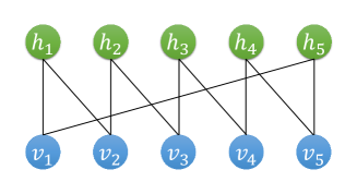
where and . A constant factor is omitted.
The structure of the RBM is shown in Fig. 1.
V Conclusion and discussions
We investigate the RBM representations of stabilizer code states and give an algorithmic way to construct the RBM parameters for a given stabilizer group . To the best of our knowledge, this is the first proof that RBMs can exactly and efficiently represent any stabilizer code state. This sheds new light on the representational power of RBMs, justifying the success of RBMs in representing highly entangled states. In the meantime, given the importance of stabilizer codes in quantum error correction, our work opens up the possibility to classically simulate quantum error-correcting code using RBMs, providing a convenient tool to initialize the code states.
Acknowledgements.
Y.-H. Zhang thanks Xiaodi Wu, Fangjun Hu and Yuanhao Wang for helpful discussions. Z.-A. Jia acknowledges Liang Kong for discussions during his stay in Yau Mathematical Sciences Center, Tsinghua University, and he also thanks Giuseppe Carleo and Rui Zhai for discussions during the first international conference on “Machine Learning and Physics” at IAS, Tsinghua university.References
- Osborne (2012) T. J. Osborne, “Hamiltonian complexity,” Reports on Progress in Physics 75, 022001 (2012).
- Verstraete (2015) F. Verstraete, “Quantum hamiltonian complexity: Worth the wait,” Nature Physics 11, 524 (2015).
- Friesdorf et al. (2015) M. Friesdorf, A. H. Werner, W. Brown, V. B. Scholz, and J. Eisert, “Many-body localization implies that eigenvectors are matrix-product states,” Phys. Rev. Lett. 114, 170505 (2015).
- Orús (2014) R. Orús, “A practical introduction to tensor networks: Matrix product states and projected entangled pair states,” Annals of Physics 349, 117 (2014).
- Verstraete et al. (2008a) F. Verstraete, V. Murg, and J. Cirac, “Matrix product states, projected entangled pair states, and variational renormalization group methods for quantum spin systems,” Advances in Physics 57, 143 (2008a), https://doi.org/10.1080/14789940801912366 .
- White (1992) S. R. White, “Density matrix formulation for quantum renormalization groups,” Phys. Rev. Lett. 69, 2863 (1992).
- Verstraete et al. (2008b) F. Verstraete, V. Murg, and J. I. Cirac, “Matrix product states, projected entangled pair states, and variational renormalization group methods for quantum spin systems,” Advances in physics 57, 143 (2008b).
- Verstraete and Cirac (2004) F. Verstraete and J. I. Cirac, “Renormalization algorithms for quantum-many body systems in two and higher dimensions,” arXiv preprint cond-mat/0407066 (2004).
- Bañuls et al. (2009) M. C. Bañuls, M. B. Hastings, F. Verstraete, and J. I. Cirac, “Matrix product states for dynamical simulation of infinite chains,” Phys. Rev. Lett. 102, 240603 (2009).
- Vidal (2007) G. Vidal, “Entanglement renormalization,” Phys. Rev. Lett. 99, 220405 (2007).
- Vidal (2003) G. Vidal, “Efficient classical simulation of slightly entangled quantum computations,” Phys. Rev. Lett. 91, 147902 (2003).
- Schuch et al. (2008) N. Schuch, M. M. Wolf, F. Verstraete, and J. I. Cirac, “Simulation of quantum many-body systems with strings of operators and monte carlo tensor contractions,” Phys. Rev. Lett. 100, 040501 (2008).
- Carleo and Troyer (2017) G. Carleo and M. Troyer, “Solving the quantum many-body problem with artificial neural networks,” Science 355, 602 (2017).
- Deng et al. (2017a) D.-L. Deng, X. Li, and S. Das Sarma, “Quantum entanglement in neural network states,” Phys. Rev. X 7, 021021 (2017a).
- Gao and Duan (2017) X. Gao and L.-M. Duan, “Efficient representation of quantum many-body states with deep neural networks,” Nature Communications 8, 662 (2017).
- Huang and Moore (2017) Y. Huang and J. E. Moore, “Neural network representation of tensor network and chiral states,” arXiv preprint arXiv:1701.06246 (2017).
- Chen et al. (2018) J. Chen, S. Cheng, H. Xie, L. Wang, and T. Xiang, “Equivalence of restricted boltzmann machines and tensor network states,” Phys. Rev. B 97, 085104 (2018).
- Glasser et al. (2018) I. Glasser, N. Pancotti, M. August, I. D. Rodriguez, and J. I. Cirac, “Neural-network quantum states, string-bond states, and chiral topological states,” Phys. Rev. X 8, 011006 (2018).
- Jia et al. (2019a) Z.-A. Jia, B. Yi, R. Zhai, Y.-C. Wu, G.-C. Guo, and G.-P. Guo, “Quantum neural network states: A brief review of methods and applications,” Advanced Quantum Technologies 2, 1800077 (2019a).
- Le Roux and Bengio (2008) N. Le Roux and Y. Bengio, “Representational power of restricted boltzmann machines and deep belief networks,” Neural computation 20, 1631 (2008).
- Deng et al. (2017b) D.-L. Deng, X. Li, and S. Das Sarma, “Machine learning topological states,” Phys. Rev. B 96, 195145 (2017b).
- Jia et al. (2019b) Z.-A. Jia, Y.-H. Zhang, Y.-C. Wu, L. Kong, G.-C. Guo, and G.-P. Guo, “Efficient machine-learning representations of a surface code with boundaries, defects, domain walls, and twists,” Phys. Rev. A 99, 012307 (2019b).
- Gottesman (1997) D. Gottesman, “Stabilizer codes and quantum error correction, caltech ph.d. thesis,” arXiv preprint quant-ph/9705052 (1997).
- Gottesman (1998) D. Gottesman, “Theory of fault-tolerant quantum computation,” Phys. Rev. A 57, 127 (1998).
- Nielsen and Chuang (2010) M. A. Nielsen and I. L. Chuang, Quantum computation and quantum information (Cambridge university press, 2010).
- Yan and Bacon (2012) J. Yan and D. Bacon, “The k-local pauli commuting hamiltonians problem is in p,” arXiv preprint arXiv:1203.3906 (2012).
- Laflamme et al. (1996) R. Laflamme, C. Miquel, J. P. Paz, and W. H. Zurek, “Perfect quantum error correcting code,” Physical Review Letters 77, 198 (1996).