August 21, 2018, Accepted September 18, 2018, Published online October 10, 2018

Effective Hamiltonian of Topological Nodal Line Semimetal in Single-Component Molecular Conductor [Pd(dddt)₂] from First-Principles

Abstract

Using first-principles density-functional theory calculations, we obtain the non-coplanar nodal loop for a single-component molecular conductor [Pd(dddt)₂] consisting of HOMO and LUMO with different parity. Focusing on two typical Dirac points, we present a model of an effective 2 $\times$ 2 matrix Hamiltonian in terms of two kinds of velocities associated with the nodal line. The base of the model is taken as HOMO and LUMO on each Dirac point, where two band energies degenerate and the off diagonal matrix element vanishes. The present model, which reasonably describes the Dirac cone in accordance with the first-principles calculation, provides a new method of analyzing electronic states of a topological nodal line semimetal.

Single-component molecular conductor, [Pd(dddt)₂], which is insulating at ambient pressure but becomes conducting and shows almost temperature independent resistivity under a pressure of 12.6 GPa, [1] has been studied using first-principles density-functional theory (DFT) calculations, [2] and linearly dispersed bands with Dirac cones were found at 8 GPa. [1, 3] An extended Hückel calculation and a tight-binding analysis of the DFT optimized structure at 8 GPa have shown nodal line semimetal. [4]. Relevant physical quantities have been examined to understand the characteristics of such new massless Dirac electron systems. [5, 6, 7, 8] In fact, the multi-orbital nature due to an interplay between HOMO (highest occupied molecular orbital) and LUMO (lowest unoccupied molecular orbital) on different molecular sites is essential for the emergence of the Dirac electron. [1] Such a state, where the contact points of the Dirac cones form a closed line (loop) called nodal line semimetal, [9, 10, 11, 12, 13] is quite different from that of massless Dirac electrons in a two-dimensional molecular conductor. [14]

In 1937, Herring [15] claimed accidental degeneracies in the energy bands followed by a closed/open circuit (nodal line) for a system with inversion symmetry. The product of parity eigenvalues at the eight time reversal invariant momentum (TRIM) determines even or odd number of circuits (nodal loop). This formula is quite similar to Fu-Kane’s criteria of $\mathbb{Z}_{2}$ topological insulator, [16] despite assuming the absence of spin-orbit coupling (SOC). However, since it should work well for weak SOC materials with light elements such as molecular conductors, the shape of the nodal line and the number of nodal loops would be useful to evaluate the band topology and design new molecular topological materials. The nodal line semimetal is a recent topic related to the new concept associated with the topological property of Dirac electrons. [17, 18, 19, 20] Among them, single nodal loop has been found in pnictides CaAg$X$ ($X$ = P and As)[21], alkaline-earth compounds of $A$$X_{2}$ ($A$ = Ca, Sr, Ba; $X$ = Si, Ge, Sn), [22] CaAs₃[23], and Ag₂S [24]. In fact, all these systems and [Pd(dddt)₂] turn out to be a strong topological insulator[25] when SOC is on. [3, 4, 26]

With the regard to the Dirac electrons in [Pd(dddt)₂], it is useful to describe the nodal line semimetal in terms of the effective Hamiltonian with a two-band model. For many nodal line semimetals, first-principles calculations have characterized the shape of the nodal line, and an effective Hamiltonian is analyzed only close to the $\Gamma$ point due to perturbation. [22, 26] However, such a Hamiltonian is insufficient to describe the large nodal line away from TRIM due to the non-coplanar [4] and snake-like loop structures. [22] Further, the model is required to show a reasonable energy band for the Dirac cone along the nodal line in order to examine the physical property, since the chemical potential (i.e., the Fermi energy) crosses the nodal line. Indeed, the model, which provides two kinds of velocity fields associated with the Dirac cone, is useful as shown by the calculation of the topological property of the Berry phase. [8] In single-band molecular conductors, first-principles band structures near the Fermi level are well reproduced by a small number of hopping parameters, [27, 28] but the corresponding parameters for a multi-band system of [Pd(dddt)₂] are huge and complicated. Therefore, a new method for the direct derivation of the model from the DFT calculation is needed to describe the Dirac cone reasonably for all the Dirac points along the loop.

In this letter, on the basis of first-principles DFT calculations, we calculate a number of Dirac points that form a single non-coplanar nodal loop centered at the $\Gamma$-point in the first Brillouin zone (BZ). The characteristics of the two crossing bands near the Dirac points and the velocities of the Dirac cone are examined by focusing on two typical Dirac points on the loop. Then, we demonstrate a new method to obtain the effective Hamiltonian for the nodal line semimetal where the base is not on the TRIM, but on the respective Dirac point. [29, 30] A model with analytical matrix elements is derived using the knowledge of the general relation between the nodal line and the velocity fields of the Dirac cone.[8]

The crystal structure of [Pd(dddt)₂], which is determined by x-ray diffraction at ambient pressure, belongs to a monoclinic system with the space group of $P2_{1}$/$a$.[1] In our previous study, using first-principles calculations, we discovered anisotropic Dirac cones of [Pd(dddt)₂] at 8GPa by performing structural optimization under symmetry operations. [1]. However, the three-dimensional characteristics of the electronic state and the effective model have not yet been reported from first-principles. The present first-principles DFT calculations are performed based on an all-electron full-potential linearized plane wave (FLAPW) method as implemented in QMD-FLAPW12. [31, 32, 33] To determine accurately the anisotropy of the Dirac cone, Fermi velocities, and contact points of Dirac cones along the nodal line, we calculate the eigenvalues around the Dirac cone by using the highly precise FLAPW method. We used a high-dense $\bm{k}$-mesh for plotting the 3D band structures. The exchange-correlation functional that is used in the present calculation is the generalized gradient approximation proposed by Perdew, Burke, and Ernzerhof. [34] The $\bm{k}$-point sampling grid of 4 $\times$ 8 $\times$ 4 was used. The BZ integration was performed with an improved tetrahedron method. [35]

Figures 1(a) and 1(b) show the band structure along the $\Gamma$-Y and along X’(-0.1967, 0, 0)-Z’(-0.1967, 0, 0.5) directions, respectively where the band crossing suggests two typical Dirac points. We refer to the former Dirac point as Dirac point (I) and the later as Dirac point (II). In general, the crossings of two linear bands with different characteristics occurs forming a Dirac cone. By comparing the characteristics of the HOMO and LUMO for the isolated [Pd(dddt)₂] monomer in Figs. 1(e) and 1(f), we discuss the wavefunction near Dirac point (I). As plotted in Figs. 1(a)–1(d), the convex upwards band predominately consists of HOMO like wavefunctions in Layer 1, and the convex downwards band is made up of LUMO like wavefunctions in Layer 2.

The shape of the Dirac cone depends on the position of the Dirac point along the nodal line. In the following, we use a wavevector scaled by $2\pi$, lattice constants of the reciprocal lattice taken as unity, and energy in the unit of eV. Figures 2(a) and 2(b) show the Dirac cone with Dirac point (I), $\bm{k}_{\rm 0}$ = (0, 0.086, 0), where the axis of the cone is parallel to a vector (–2^-1/2, 0, 2^-1/2). The principal axes of the plane, which are perpendicular to the axis of the Dirac cone, are given by a*+c* ($k_{x+z}$) and b* ($k_{y}$). Dirac cone (I) shown in Fig. 2(a) is symmetric with respect to $k_{x+z}$ while that shown in Fig. 2(b) is tilted along the positive $k_{y}$. Figures 2(c) and (d) show the Dirac cone of Dirac point (II), $\bm{k}_{\rm 0}$ = (-0.1967, 0.000, 0.3924), where the axis of the cone is parallel to b* ($k_{y}$). The former shows a bird’s eye view with tilting along both $k_{x}$ and $k_{z}$ axes. The latter denotes the gap function around Dirac point (II), which is the difference in energy between the valence and conduction bands, $E_{c}(\bm{k})-E_{v}(\bm{k})$. The principal axes of the Dirac cone (II) is rotated counterclockwise with an angle $\theta\sim\tan^{-1}(0.2)$ and the tilting does not appear. The difference in behavior of the Dirac cone between Dirac points (I) and (II) is discussed in terms of the effective Hamiltonian.

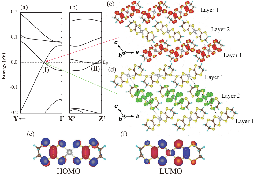
Figure 1: (Color online) Band structure of [Pd(dddt)₂] at 8GPa (without SOC) along the $\Gamma$-Y direction (a) and along the X’(-0.1967, 0, 0)-Z’(-0.1967, 0, 0.5) direction (b) on which Dirac points (I) and (II) are found, respectively. Wavefunction at a fixed $\bm{k}$: charge densities $|\Psi_{i,\bm{k}}|^{2}$ close to Dirac point (I) for the bottom of the conduction bands (c), and those at the top for the valence bands (d). The notations a, b, and c denote the respective lattice vectors of the unit cell. Contour plot of the orbital (charge) density of the HOMO (e) and LUMO (f) of isolated [Pd(dddt)₂] monomer.

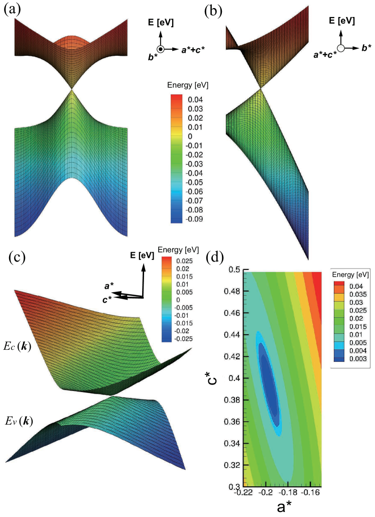
Figure 2: (Color online) Band structure close to Dirac point (I) on the $k_{x+z}$-$k_{y}$ plane, where (a) and (b) are the side views with the horizontal axis given by b* with $0.06~{}<~{}k_{y}~{}<~{}0.122$ and by a*+c* with $-0.2<k_{x+z}<0.2$, respectively. (c) Bird’s eye view of the Dirac cone with apex at Dirac point (II) on the $k_{x}$-$k_{z}$ plane, where $-0.22<k_{x}<-0.15$ and $0.3<k_{z}<0.5$. (d) 2D contour plots corresponding to (c) for the difference in energy between the top of the valence bands, $E_{v}$($\bm{k}$), and the bottom of conduction bands, $E_{c}$($\bm{k}$), on the a*-c* plane, where $k_{x}$ and $k_{z}$ represent a* and c*, respectively, which are taken as the orthogonal axes, for simplicity.

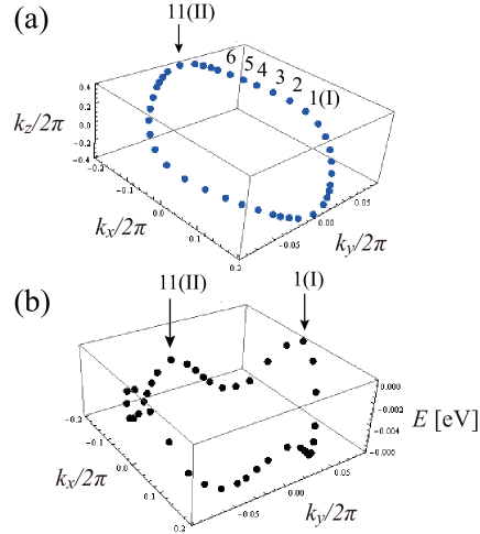
Figure 3: (Color online) (a) Nodal line of accidental degeneracies in [Pd(dddt)₂] at 8GPa. The loop is formed by the trajectory of the contact points of Dirac cones in the three-dimensional momentum space, $(k_{x},k_{y},k_{z})$ in the absence of spin-orbit coupling. The locations of the respective points on the line, which are scaled by $2\pi$ $\bm{k}_{\rm 0}[=(k_{\rm 0x},k_{\rm 0y},k_{\rm 0z})]$ are given by (0, 0.086, 0) (1), (-0.042, 0.083, 0.05) (2), (-0.078, 0.0755, 0.1) (3), (-0.109, 0.066, 0.15) (4), (-0.131, 0.057, 0.2) (5), (-0.151, 0.047, 0.25) (6), (-0.168, 0.037, 0.3) (7), (-0.176, 0.0315, 0.325) (8), (-0.184, 0.0245, 0.35) (9), (-0.191, 0.0165, 0.375) (10), and (-0.1967, 0.000, 0.3924) (11) where we mainly examine the symmetric points (1) and (11) defined by (I) and (II) respectively. (b) The corresponding energy dispersion of the nodal line, $E(\bm{k})$ [eV]. The origin of the energy is set to be the energy at Dirac point (I). The energy is the same for Dirac points shown by $\bm{k}_{\rm 0}$ = $(k_{\rm 0x},\pm k_{\rm 0y},k_{\rm 0z})$ and $(-k_{\rm 0x},\pm k_{\rm 0y},-k_{\rm 0z})$.

Figure 3(a) shows the nodal line (trajectory of Dirac points) of [Pd(dddt)₂] at 8 GPa, which consists of 11 independent Dirac points $\bm{k}_{\rm 0}$ calculated using the first-principles calculations. Note that the present DFT calculations show a non-coplanar loop within the first BZ, while the loop of the previous tight-binding model [4] extends over the first BZ. For the estimation of the effective Hamiltonian, we focus on Dirac points (I) and (II) represented by the numbers 1 and 11, respectively. The trajectory of the Dirac points suggests an accidental degeneracy, which occurs without the symmetry of the crystal. Note that these Dirac points are symmetric with respect to the $\Gamma$-point and the plane of $k_{y}=0$ ($k_{x}$–$k_{z}$ is a mirror plane), respectively.

Using Fig. 3(a), we examine the effective Hamiltonian of a two-band model, where the base is given by the respective Dirac point $\bm{k}_{\rm 0}$. Note that this method describes the Dirac cone correctly, as shown in Refs. Luttinger1955 and  Kobayashi2007_JPSJ. Two energies consisting of different kinds of parities degenerate on the Dirac point, where arbitrary linear combination of these two wavefunctions becomes possible. The eigenfunctions with $\bm{k}$, which is just away from the Dirac point is determined uniquely, and their linear combination rotates around the Dirac point.[36] In the present case, we can choose two eigenfunctions of HOMO and LUMO with different symmetry at the Dirac point.

Now we derive the effective Hamiltonian of the two band model explicitly. We start with the full 8 $\times$ 8 Hamiltonian that is represented at the $\Gamma$-point. Such a Hamiltonina is given by

$$H(\bm{k}) = \begin{pmatrix}H^{\rm HH}(\bm{k})&H^{\rm HL}(\bm{k})\\ H^{\rm LH}(\bm{k})&H^{\rm LL}(\bm{k})\end{pmatrix}\ ,$$ (1)

where the 4 $\times$ 4 matrix $H^{\rm HH}(\bm{k})$ ( $H^{\rm LL}(\bm{k})$) consists of only HOMO (LUMO) and $H^{\rm HL}(\bm{k})$ ($H^{\rm HL}(\bm{k})$) denotes the interaction between HOMO and LUMO. The former is the even function of $\bm{k}$ due to the time reversal symmetry, while the latter is the odd function due to interaction with different parity. Among the energy bands of the four HOMOs and four LUMOs, we choose two bands given by the top HOMO bands and the bottom LUMO bands, which are assumed to be isolated from the other bands. The Scrödinger equation for these two bands $E_{\rm H}(\bm{k}$) and $E_{\rm L}(\bm{k})$ is given by

$$H^{0}(\bm{k})|H(L)(\bm{k})>=E_{\rm H(L)}(\bm{k})|H(L)(\bm{k})>\;,$$ (2)

where $H^{0}({\bm{k}})$ denotes Eq. (1) without $H^{\rm HL}(\bm{k})$ and $H^{\rm LH}(\bm{k})$. By using $|H(\bm{k})>$ and $|L(\bm{k})>$, the reduced Hamiltonian of the 2 $\times$ 2 matrix is written as

$$H^{\rm red} = \sum_{\alpha,\beta={\rm H},{\rm L}}|\alpha(\bm{k})><\alpha(\bm{k})|H(\bm{k})|\beta(\bm{k})><\beta(\bm{k})|$$ (3)

$$=\sum_{\alpha,\beta={\rm H},{\rm L}}|\alpha(\bm{k})>H_{\rm eff}<\beta(\bm{k})|\;.$$

By defining

$$f_{0} = (E_{\rm H}(\bm{k})+E_{\rm L}(\bm{k})|/2\;,$$

$$f_{3} = |E_{\rm H}(\bm{k})-E_{\rm L}(\bm{k})|/2\;,$$

$$f_{2} = i<{\rm H}(\bm{k})|H|{\rm L}(\bm{k})>\;,$$ (4)

$H_{\rm eff}(\bm{k})$ in Eq. (3) is expressed as

$${H_{\rm eff}(\bm{k})} = \begin{pmatrix}f_{0}(\bm{k})+f_{3}(\bm{k})&-if_{2}(\bm{k})\\ if_{2}(\bm{k})&f_{0}(\bm{k})-f_{3}(\bm{k})\end{pmatrix}\ ,$$ (5)

where $\bm{k}=(k_{x},k_{y},k_{z})$ and $f_{0}(0)$ is taken as zero. The energy is given by $E_{\pm}=f_{0}\pm\sqrt{f_{2}^{2}+f_{3}^{2}}$, where $E_{+}(E_{-})=E_{c}(E_{v})$. The Dirac point $\bm{k}_{\rm 0}$ on the nodal line is obtained from

$$f_{2}(\bm{k}_{\rm 0}) = 0\;,$$ (6a)

$$f_{3}(\bm{k}_{\rm 0}) = 0\;.$$ (6b)

Note that $f_{0}(\bm{k})$ and $f_{3}(\bm{k})$ are the even functions of $\bm{k}$ due to time reversal symmetry. The quantity $f_{2}(\bm{k})$, which is also real due to the presence of inversion symmetry around the Pd atom, [4] is the odd function of $\bm{k}$ due to HOMO and LUMO having different parities. The function $f_{2}(\bm{k})$ is estimated by projecting the nodal line on the $k_{x}$ - $k_{z}$ plane in Fig. 4(a), while $f_{3}(\bm{k})$ is estimated by projecting the nodal line on the $k_{x}$ - $k_{y}$ plane in Fig. 4(b). This method reproduces the Dirac points well as shown in Fig. 3(a). We empirically examined the form under the constraint that the Dirac points (0, 0.086, 0) (I) and (-0.1967, 0.000, 0.3924) (II) satisfy Eqs. (6a) and (6b).These functions are obtained as

$$f_{2}(\bm{k}) \simeq C_{2}(k_{z}+k_{x}+40k_{x}^{3}-380k_{x}^{5})\;,$$ (7a)

$$f_{3}(\bm{k}) \simeq C_{3}((k_{x}/0.1967)^{2}+(k_{y}/0.086)^{2}$$ (7b)

$$+(k_{x}k_{y}/0.027)^{2}-1)\;,$$

$$f_{0}(\bm{k}) \simeq b_{x}k_{x}^{2}+b_{y}k_{y}^{2}+b_{z}k_{z}^{2}+C_{0}\;.$$ (7c)

where the velocity of the cone at the Dirac point $\bm{k}_{\rm 0}$ is obtained as $\bm{v}_{2}=\nabla_{\bm{k}_{\rm 0}}f_{2}$, $\bm{v}_{3}=\nabla_{\bm{k}_{\rm 0}}f_{3}$ and $\bm{v}_{0}=\nabla_{\bm{k}_{\rm 0}}f_{0}$ corresponding to the tilting. Using $\bm{k}_{\rm 0}=(k_{\rm 0x},k_{\rm 0y},k_{\rm 0z})$, $\bm{v}_{j}$ is calculated as

$$\bm{v}_{2} = \nabla_{\bm{k}_{\rm 0}}f_{2}\simeq C_{2}(1+120k_{\rm 0x}^{2}-2280k_{\rm 0x}^{4},0,1),$$ (8a)

$$\bm{v}_{3} = \nabla_{\bm{k}_{\rm 0}}f_{3}\simeq C_{3}(2k_{\rm 0x}/0.196^{2}+2k_{\rm 0x}k_{\rm 0y}^{2}/0.027^{2},$$ (8b)

$$2k_{\rm 0y}/0.086^{2}+2k_{\rm 0x}^{2}k_{\rm 0y}/0.027^{2},0)\;,$$

$$\bm{v}_{0} = \nabla_{\bm{k}_{\rm 0}}f_{0}\simeq(2b_{x}k_{\rm 0x},2b_{y}k_{\rm 0y},2b_{z}k_{\rm 0z})\;.$$ (8c)

Note that the tangent of the nodal line is parallel to $\bm{v}_{2}\times\bm{v}_{3}$.[8] In the previous work,[30] $\bm{v}_{j}$ was estimated directly from Eq. (4) using the wavefunction close to $\bm{k}=\bm{k}_{\rm 0}$. From $f_{j}(\bm{k})-f_{j}(\bm{k}_{\rm 0})\simeq\bm{v}_{j}\cdot\delta\bm{k}$, ($j$ = 2, 3, 0) with $\delta\bm{k}=\bm{k}-\bm{k}_{\rm 0}$, the energy of the Dirac cone is given by $E_{\pm}(\bm{k})-E(\bm{k}_{\rm 0})\simeq\bm{v}_{0}\cdot\delta\bm{k}$ $\pm\sqrt{(\bm{v}_{2}\cdot\delta\bm{k})^{2}+(\bm{v}_{3}\cdot\delta\bm{k})^{2}}$. The coefficients of $k_{x}^{3}$, $k_{x}^{5}$ and $(k_{x}k_{y})^{2}$ in Eqs. (7a) and (7b) are determined by fitting the line to the other $\bm{k}_{\rm 0}$. As shown in Figs. 4(a) and 4(b), good coincidence is obtained for both $f_{2}(\bm{k})$ and $f_{3}(\bm{k})$ where $f_{2}(\bm{k})$ reflects the symmetry of $k_{y}$=0. The arrow in the inset of Fig. 4(a) represents $\bm{v}_{2}$ at Dirac point (I) which is perpendicular to $f_{2}(\bm{k})$ (solid line). Coefficients $C_{2}$, $C_{3}$, $b_{x}$, $b_{y}$, and $b_{z}$ are calculated as follows.

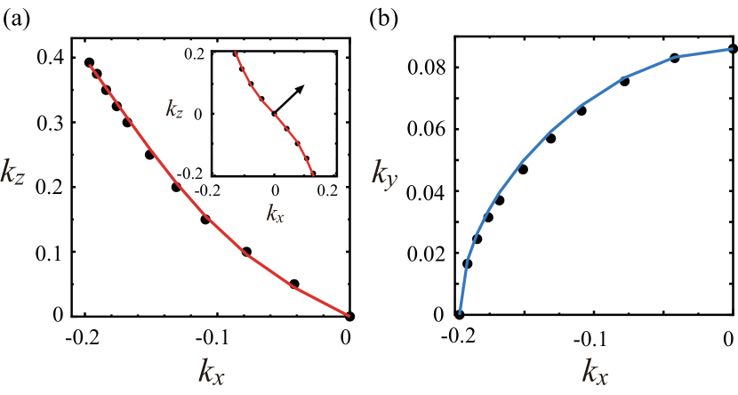
Figure 4: (Color online) Dirac points (symbols) projected on the $k_{x}$ - $k_{z}$ plane (a) and $k_{x}$ - $k_{y}$ plane (b), which are used to obtain the fitting lines for $f_{2}(\bm{k})$ and $f_{3}(\bm{k})$ (Eqs. (7a) and (7b)), respectively. The inset shows $f_{2}(\bm{k})$ around the $\Gamma$-point. The arrow, which depicts $\bm{v}_{2}$ at Dirac point (I) with arbitrary scale, corresponds to the horizontal axis a*+c* in Fig. 2(a).

First, we examine the Dirac cone at Dirac point (I) where $\bm{v}_{2}=C_{2}(1,0,1)$, $\bm{v}_{3}=C_{3}(0,1,0)$, and $\bm{v}_{0}=2b_{y}k_{\rm 0y}(0,1,0)$. Noting $\bm{v}_{2}\cdot\bm{v}_{3}$ = 0, the principal axes are given by $k_{x}$+$k_{z}$ and $k_{y}$. By comparing the velocities with those of Figs. 2(a) and 2(b), which give

$$v_{2} = \bm{v}_{2}\cdot(2^{-1/2},0,2^{-1/2})=0.21\;,$$ (9a)

$$v_{y} = \bm{v}_{3}\cdot(0,1,0)\pm\bm{v}_{0}\cdot(0,1,0)=1.25\pm 0.45\;,$$

we obtain $C_{2}\simeq 0.148$, $b_{y}\simeq-2.6$, and $C_{3}\simeq 0.053$. Coefficients $C_{2}$ and $C_{3}$ can also be obtained from the gap $E_{c}(\bm{k})-E_{v}(\bm{k})$ at the $\Gamma$-point and Z-point, which are estimated as 0.0994 and 0.1117, respectively. The resultant quantities $C_{2}$ = 0.137 and $C_{3}$ = 0.050 are compatible with those of Eqs. (9a) and (9), which suggests that the effective Hamiltonian of Eq. (5) is valid not only for $\bm{k}$ close to the nodal line but also for the extended regions including the $\Gamma$- and Z-points.

Next, we examine the Dirac cone at Dirac point (II) to verify the validity of Eqs. (7a) and (7a) with $C_{2}=0.148$ and $C_{3}=0.053$. The Dirac cone is shown on the plane of $k_{x}$ - $k_{z}$, but the principal axes do not coincide with that of $\bm{v}_{2}$ and $\bm{v}_{3}$ since $\bm{v}_{2}\cdot\bm{v}_{3}\not=0$ from Eqs. (8a) and (8a). We estimate the gap function given by $2\Delta(\bm{k})=E_{c}(\bm{k})-E_{v}(\bm{k})$ $=2\sqrt{(\bm{v}_{2}\cdot\delta\bm{k})^{2}+(\bm{v}_{3}\cdot\delta\bm{k})^{2}}$ with $\delta\bm{k}=(x,0,z)$, which is calculated as $(E_{c}(\bm{k})-E_{v}(\bm{k}))^{2}/4=0.45x^{2}+0.117xz+0.02z^{2}$ $(=Ax^{2}+2Cxz+Bz^{2})$. This shows the rotation of the principal axes from $(x,z)$ to $(X,Z)$, where $x=X\cos\theta-Z\sin\theta$, and $z=X\sin\theta+Z\cos\theta$. In terms of $(X,Z)$, the gap function is expressed as

$$\Delta(\bm{k})^{2}=\Delta(\delta\bm{k}+\bm{k}_{\rm 0})=Ax^{2}+2Cxz+Bz^{2}=$$

$$\frac{1}{2}\left(A+B+\sqrt{(A-B)^{2}+4C^{2}}\right)X^{2}$$

$$+\frac{1}{2}\left(A+B-\sqrt{(A-B)^{2}+4C^{2}}\right)Z^{2}\;,$$

$$\tan(2\theta)=\frac{2C}{A-B}\;.$$ (10)

The cross section of $\Delta(\bm{k})=E_{0}$ shows an ellipse with the radius of the minor [major] axis given by $a=2^{1/2}E_{0}/\sqrt{A+B+((A-B)^{2}+4C^{2})^{1/2}}$ [$b$ = $2^{1/2}E_{0}/\sqrt{A+B-((A-B)^{2}+4C^{2})^{1/2}}$], which is rotated by an angle $\theta=2^{-1}\tan^{-1}[2C/(A-B))]$. The radius and angle for Dirac point (II) are obtained as $a=1.5E_{0}$, $b=8.5E_{0}$, $b/a\simeq 5.6$ and $\tan\theta=0.13$, which correspond well to the numerical result in Fig. 2(d), i.e., $b/a\simeq 7$ and $\tan\theta\simeq 0.2$. Therefore, our Hamiltonian may be applied to all the Dirac points between points (I) and (II).

Further, from Eq. (10), we estimate the area of the ellipse $S$ with the gap $2E_{0}$ for an arbitrary Dirac point, where the axis of the cone is parallel to the tangent of the nodal line ( i.e., $\propto\bm{v}_{2}\times\bm{v}_{3}$) and the wavefunction of the Dirac cone is determined by $\bm{v}_{2}$ and $\bm{v}_{3}$. By taking the axis of the cone as $y$ and the plane of the cone as the $x$ - $z$ plane, we obtain the area of the ellipse $S$ with the gap $2E_{0}$ as $S(\bm{k}_{\rm 0})=\pi ab$ $=\pi E_{0}^{2}/\sqrt{AB-C^{2}}=\pi E_{0}^{2}/|\bm{v}_{2}(\bm{k}_{\rm 0})\times\bm{v}_{3}(\bm{k}_{\rm 0})|$, where $\bm{v}_{2}=(v_{2x},0,v_{2z})$, $\bm{v}_{3}=(v_{3x},0,v_{3z})$, $A=v_{2x}^{2}+v_{3x}^{2}$, $B=v_{2z}^{2}+v_{3z}^{2}$, and $C=v_{2x}v_{2z}v_{3x}v_{3z}$. We note that $\bm{v}_{2}\cdot\bm{v}_{3}\not=0$ is generally expected except for Dirac point (I), which is located on the symmetric line of $\Gamma$ - Y.

Finally, we calculate $b_{x}$ and $b_{z}$ in Eq. (7c) from Dirac cone (II), which gives $v_{x}=0.36\pm 0.12$ and $v_{z}=0.09\pm 0.06$. In a way similar to Eqs. (9a) and (9), we obtain $b_{x}\simeq-0.30$ and $b_{z}\simeq 0.077$ suggesting that the tilting occurs towards the negative (negative) direction for the $k_{x}$ ($k_{z}$) axis. This is qualitatively consistent with Fig. 2(c). As shown in Fig. 3(b), our DFT calculation of the energy difference measured from that of Dirac point (I) exhibits nonmonotonical behavior, e.g., -0.0031, -0.0061, -0.0059, -0.0047, and -0.0032 eV for the nodal points No. 3, 5, 7, 9, and 11 in Fig. 3(a), respectively. However, it is quite complicated to reproduce the dispersion quantitatively from Eq. (7c) with a constant $C_{0}$, and such a problem becomes an issue to be solved in the next step.

Here, it should be noted that the SOC was ignored in the present calculation. Since the crystal structure is centrosymmetric, the band structures are in Kramers degeneracy. Then, the loop degeneracies are destroyed by the SOC, leading to an energy gap with $\simeq$ 3 meV at Dirac point (I), [3] which will be examined further.

We comment on the experiment in which the present model is useful for performing the analysis. Since all the directions for the nodal line can be treated on the same footing, the effect of magnetic field is of interest to examine the characteristic behavior of the Landau level. The Hall coefficient is also expected to exhibit anisotropic behavior.

In summary, we performed first-principles calculations for [Pd(dddt)₂] at 8GPa, and found a non-coplanar nodal loop within the first BZ. The present effective Hamiltonian obtained from the Dirac points in Fig. 3(a) describes well the electron close to the nodal line. The explicit form of the velocity is obtained by Eqs. (8a)-(8c), with $C_{2}\simeq 0.148,C_{3}\simeq 0.05,b_{x}\simeq-0.31,b_{y}\simeq-2.6$, and $b_{z}\simeq 0.077$, which are useful for future calculations of transport.

- [1] R. Kato, H. Cui, T. Tsumuraya, T. Miyazaki, and Y. Suzumura, J. Am. Chem. Soc. 139, 1770 (2017).
- [2] W. Kohn and L. J. Sham, Phys. Rev. 140, A1133 (1965).
- [3] T. Tsumuraya, H. Sawahata, F. Ishii, H. Kino, R. Kato, and T. Miyazaki, Am. Phys. Soc. Bull, R14.00012 (2018).
- [4] R. Kato and Y. Suzumura, J. Phys. Soc. Jpn. 86, 064705 (2017).
- [5] Y. Suzumura and R. Kato, Jpn. J. Appl. Phys. 56, 05FB02 (2017).
- [6] Y. Suzumura, J. Phys. Soc. Jpn. 86, 124710 (2017).
- [7] Y. Suzumura, H. Cui, and R. Kato, J. Phys. Soc. Jpn. 87, 084702 (2018).
- [8] Y. Suzumura and A. Yamakage, J. Phys. Soc. Jpn. 87(9), 093704 (2018).
- [9] Y. Kim, B. J. Wieder, C. L. Kane, and A. M. Rappe, Phys. Rev. Lett. 115, 036806 (2015).
- [10] H. Weng, Y. Liang, Q. Xu, R. Yu, Z. Fang, X. Dai, and Y. Kawazoe, Phys. Rev. B 92, 045108 (2015).
- [11] K. Mullen, B. Uchoa, and D. T. Glatzhofer, Phys. Rev. Lett. 115, 026403 (2015).
- [12] C. Fang, Y. Chen, H.-Y. Kee, and L. Fu, Phys. Rev. B 92, 081201 (2015).
- [13] J. Liu and L. Balents, Phys. Rev. B 95, 075426 (2017).
- [14] S. Katayama, A. Kobayashi, and Y. Suzumura, J. Phys. Soc. Jpn. 75, 054705 (2006).
- [15] C. Herring, Phys. Rev. 52, 365 (1937).
- [16] L. Fu and C. L. Kane, Phys. Rev. B 76, 045302 (2007).
- [17] S. Murakami, New J. Phys. 9, 356 (2007).
- [18] A. A. Burkov, M. D. Hook, and L. Balents, Phys. Rev. B 84, 235126 (2011).
- [19] M. Hirayama, R. Okugawa, T. Miyake, and S. Murakami, Nat. Commun. 8, 14022 (2017).
- [20] M. Hirayama, R. Okugawa, and S. Murakami, J. Phys. Soc. Jpn 87, 041002 (2018).
- [21] A. Yamakage, Y. Yamakawa, Y. Tanaka, and Y. Okamoto, J. Phys. Soc. Jpn. 85, 013708 (2016).
- [22] H. Huang, J. Liu, D. Vanderbilt, and W. Duan, Phys. Rev. B 93, 201114 (2016).
- [23] Y. Quan, Z. P. Yin, and W. E. Pickett, Phys. Rev. Lett. 118, 176402 (2017).
- [24] H. Huang, K.-H. Jin, and F. Liu, Phys. Rev. B 96, 115106 (2017).
- [25] L. Fu, C. L. Kane, and E. J. Mele, Phys. Rev. Lett. 98, 106803 (2007).
- [26] Z. Liu, H. Wang, Z. F. Wang, J. Yang, and F. Liu, Phys. Rev. B 97, 155138 (2018).
- [27] H. Kino and T. Miyazaki, J. Phys. Soc. Jpn. 75, 034704 (2006).
- [28] T. Koretsune and C. Hotta, Phys. Rev. B 89, 045102 (2014).
- [29] J. M. Luttinger and W. Kohn, Phys. Rev. 97, 869 (1955).
- [30] A. Kobayashi, S. Katayama, Y. Suzumura, and H. Fukuyama, J. Phys. Soc. Jpn. 76, 034711 (2007).
- [31] E. Wimmer, H. Krakauer, M. Weinert, and A. J. Freeman, Phys. Rev. B 24(2), 864 (1981).
- [32] D. D. Koelling and G. O. Arbman, J. Phys. F, Metal Phys. 5, 2041 (1975).
- [33] M. Weinert, J. Math. Phys. 22, 2433 (1981).
- [34] J. P. Perdew, K. Burke, and M. Ernzerhof, Phys. Rev. Lett. 77, 3865 (1996).
- [35] P. E. Blöchl, O. Jepsen, and O. K. Andersen, Phys. Rev. B 49, 16223 (1994).
- [36] S. Katayama, A. Kobayashi, and Y. Suzumura, Eur. Phys. J. B 67, 139 (2009).