Stable Optical Rigidity Based on Dissipative Coupling

Abstract

We show that the stable optical rigidity can be obtained in a Fabry-Perot cavity with dissipative optomechanical coupling and with detuned pump, corresponding conditions are formulated. An optical detection of a weak classical mechanical force with usage of this rigidity is analyzed. The sensitivity of small force measurement can be better than the standard quantum limit (SQL).

I Introduction

Resonant optomechanics Aspelmeyer et al. (2014) investigates interaction between an optical cavity and a free mass or a mechanical oscillator. The simplest optomechanical interaction is based on the radiation pressure effect in which a force proportional to optical power or number of the optical quanta, circulating in a 1D optical cavity, acts on a test mass so that the size of the optical cavity increases with increase of number of the optical quanta localized in there. Such interaction is usually called as dispersive coupling. Systems having several degrees of freedom allow more complex optomechanical interactions, including radiation pulling (negative radiation pressure) Povinelli et al. (2005); Maslov et al. (2013), optomechanical interaction proportional to the quadrature of electromagnetic field S.P. Vyatchanin and A.B. Matsko (1993, 1996); A.B. Matsko and S.P. Vyatchanin (1997); H.J. Kimble et al. (2001) and the interaction depending on the speed and not the coordinate of the mechanical system V.B. Braginsky and F.Ya. Khalili. (1990); V.B. Braginsky et al. (2000).

Optomechanical interaction is important in precise measurements which use an efficient quantum transduction mechanism between the mechanical and optical degrees of freedom allowing various sensors, like gravitational wave detectors LVC-Collaboration (2013); Aso et al. (2013); Dooley et al. (2014); C.Affeld et al. (2104); J. Aasi et al et al.(2015) (LIGO Scientific Collaboration); F. Acernese et al, (2015) (Virgo Collaboration); B.P. Abbott et al, (2018) (LIGO Scientific Collaboration, Virgo Collaboration and KAGRA Collaboration); B. P. Abbott et al, (2016) (LIGO Scientific Collaboration and Virgo Collaboration); B.P. Abbott et al, (2017a) (LIGO Scientific Collaboration and Virgo Collaboration); B.P. Abbott et al, (2017b) (LIGO Scientific Collaboration and Virgo Collaboration); F. Acernese et al (2018) (Virgo Collaboration), torque sensors M. Wu et al. (2014), and magnetometers S. Forstner and S. Prams and J. Knittel and E.D. van Ooijen and J.D. Swaim and G.I. Harris and A. Szorkovszky and W.P. Bowen and H. Rubinsztein-Dunlop (2012).

Sensitivity of the mechanical coordinate measurement in an optomechanical system usually is restricted by the so-called standard quantum limit (SQL) V.B. Braginsky (1968); V.B. Braginsky and F.Ya. Khalili (1992) due to the quantum backaction. The SQL was investigated in various configurations ranging from the macroscopic gravitational wave detectors H.J. Kimble et al. (2001) to the microcavities Kippenberg and Vahala (2008); J.M. Dobrindt and T.J. Kippenberg (2010). Sensitivity of the other types of measurements being derivatives of the coordinate detection is also limited by the SQL. An example of such measurement is detection of a classical force acting on a mechanical degree of freedom of an optomechanical system. However, the SQL of the force measurement is not an unavoidable limit. Several approaches can surpass the SQL, for example, variational measurement S.P. Vyatchanin and A.B. Matsko (1993); Vyatchanin and Zubova (1995); H.J. Kimble et al. (2001), optomechanical velocity measurement using dispersive coupling V.B. Braginsky and F.Ya. Khalili. (1990); V.B. Braginsky et al. (2000), measurements in optomechanical systems with optical rigidity V.B. Braginsky and F.Ya. Khalili (1999); F.Ya. Khalili (2001). Quantum speed meter based on dissipative coupling was proposed recently S.P. Vyatchanin and A.B. Matsko (2016).

Among variety of the optomechanical interactions the dissipative coupling takes a special place. The dissipative coupling is characterized by dependence of an optic cavity relaxation on a mechanical coordinate (in case of a Fabry-Perot cavity the mechanical coordinate changes transparency of the input mirror), whereas dispersive coupling is characterized by the dependence of a cavity frequency on the coordinate. The system with dissipative coupling cannot be considered lossless anymore. But the dissipation here does not lead to decoherence or absorption of light, instead, it results in lossless coupling between a continuous optical wave and a mode of an optical cavity. The cavity with dissipative coupling can be used as a perfect transducer between the continuous optical wave and the mechanical degree of freedom, allowing efficient cooling of the mechanical oscillator F. Elste and S.M. Girvin and A.A. Clerk (2009); M. Li and W.H.P. Pernice and H.X. Tang (2009); M. Wu et al. (2014); Hryciw et al. (2015); Sawadsky et al. (2015), exchange of the quantum states between the optical and mechanical degrees of freedom, mechanical squeezing A. Kronwald and F. Marquardt and A.A. Clerk (2013); Tan et al. (2013); Zhu et al. (2014); K. Qu and G.S. Agarwal (2015), and a combination of cooling and squeezing W.G. Gu and G.X. Li and Y.P. Yang (2013); Gu and Li (2013). A combination of conventional, dispersive, and dissipative coupling adds more complexity to the interaction and leads to the new effects S. Huang and G.S. Agarwal (2010a, b).

Dissipative coupling was proposed theoretically F. Elste and S.M. Girvin and A.A. Clerk (2009) and implemented experimentally about ten years ago M. Li and W.H.P. Pernice and H.X. Tang (2009); Weiss et al. (2013); M. Wu et al. (2014); Hryciw et al. (2015). It was investigated in different optomechanical systems, including a Fabry-Perot interferometer M. Li and W.H.P. Pernice and H.X. Tang (2009); Weiss et al. (2013); M. Wu et al. (2014); Hryciw et al. (2015), a Michelson-Sagnac interferometer (MSI) Xuereb et al. (2011); Tarabrin et al. (2013); Sawadsky et al. (2015), and the ring resonators S. Huang and G.S. Agarwal (2010a, b).

In this paper we report on one more important feature of a cavity with dissipative coupling. Such cavity, non-resonantly pumped, introduces a stable optical rigidity into the mechanical degree of freedom. Recall that the optical rigidity based on conventional dispersive coupling (in non-resolved side band case) is unstable and can be used only with feedback. We formulate the conditions of stability and show that the stable optical rigidity based on dissipative coupling allows to surpass the SQL.

II Hamiltonian approach

We consider a 1D optomechanical cavity presented on Fig. 1, it’s optical mode with eigenfrequency $\omega_{0}$ is pumped with the detuned light (the pump frequency $\omega_{p}=\omega_{0}+\delta$) — it is generalization of the model in S.P. Vyatchanin and A.B. Matsko (2016). The optical mode is dissipatively coupled with a mechanical system represented by a free test mass $m$. Relaxation rate $\kappa$ of the optical mode depends on the displacement $x$ of the test mass. The force of interest $F_{s}$ acts on the test mass and changes it’s position.

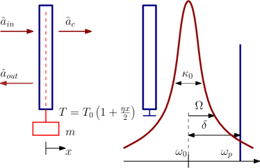
Figure 1: Scheme of the Fabry-Perot cavity dissipatively coupled with displacement $x$ of free mass $m$. The coupling changes the linear amplitude transmittance of the cavity front mirror $T(x)=T_{0}\big{[}1+\frac{\eta x}{2}\big{]}$ (2c), where $T_{0}$ is the unperturbed amplitude transmission coefficient related to full width at the half maximum of the mode as $\kappa_{0}=T_{0}^{2}/\tau$, where $\tau$ is the round trip time of the light in the cavity. The optical mode is pumped with the detuned coherent light ($\omega_{p}=\omega_{0}+\delta$).

We use the Hamiltonian approach to describe the dissipative coupling following A.A. Clerk and M.H. Devoret and S.M. Girvin and F. Marquardt and R.J. Schoelkopf (2010); S.P. Vyatchanin and A.B. Matsko (2016):

$$H =\hslash\omega_{0}\hat{a}_{c}^{\dagger}\hat{a}_{c}+\frac{\hat{p}^{2}}{2m}+H_{T}+H_{\kappa}-F_{s}\hat{x},$$ (1)

where $\hat{a}_{c}$ and $\hat{a}_{c}^{\dagger}$ are the annihilation and creation operators describing the intracavity optical field, $\hat{p}$ is the momentum of the free test mass, $H_{T}$ describes electromagnetic continuum Marquardt and Girvin (2009); Aspelmeyer et al. (2014), $H_{\kappa}$ stands for attenuation of the pump photons and associated quantum noise. From the Hamiltonian (1) we obtain the set of corresponding equations describing time evolution of the optomechanical system

$$\dot{\hat{a}}+ \left(\frac{\kappa}{2}-i\delta\right)\hat{a}=\sqrt{\kappa}\,\hat{a}_{in},$$ (2a)

$$\ddot{\hat{x}} =i\hslash\frac{\sqrt{\kappa_{0}}\eta}{2m}\left[\hat{a}^{\dagger}\hat{a}_{in}-\hat{a}_{in}^{\dagger}\hat{a}\right]+\frac{F_{s}}{m},$$ (2b)

$$\kappa=\kappa_{0}(1+\eta\hat{x}),\;\sqrt{\kappa}\simeq\sqrt{\kappa_{0}}\left(1+\frac{\eta}{2}\hat{x}\right),$$ (2c)

Here $$\hat{a} \hat{a}_{c}=\hat{a}e^{-i\omega_{p}t} \kappa x \eta \hat{a}_{in}$$ is the slow amplitude (, see (50c)) of the intracavity wave, is full width at the half maximum of the mode (relaxation rate) depending on the position of the test mass and is a constant of dissipative coupling, is the slow amplitude of the input wave, see details in Appendix A.

These equations have to be supplied with an expression for the output amplitude $\hat{a}_{out}$, which can be written in the case of small transparency $T_{0}\ll 1$ as

$$\hat{a}_{out} =-\hat{a}_{in}+\sqrt{\kappa}\,\hat{a}.$$ (2d)

Below we present amplitudes as a sum of large mean and small addition values

$$\hat{a} \Rightarrow A+\hat{a},\quad\hat{a}_{in}\Rightarrow A_{in}+\hat{a}_{in},\quad\hat{a}_{out}\Rightarrow A_{out}+\hat{a}_{out}$$

where $A,\,A_{in}$ and $A_{out}$ are expectation values of amplitudes of the intracavity, pump and reflected waves, $\hat{a}_{in}$ is vacuum fluctuation wave falling on cavity, which commutator and correlator are the following

$$\left[\hat{a}_{in}(t),\hat{a}_{in}^{\dagger}(t^{\prime})\right] =\delta(t-t^{\prime}),$$ (3)

$$\left\langle\hat{a}_{in}(t)\hat{a}_{in}^{\dagger}(t^{\prime})\right\rangle =\delta(t-t^{\prime})$$ (4)

We assume that the expectation values exceed the fluctuation parts of the operators:

$$A\gg\hat{a},\quad A_{in}\gg\hat{a}_{in},\quad A_{out}\gg\hat{a}_{out}$$ (5)

and apply the method of successive approximations below.

Recall that from this point by $\hat{a},\,\hat{a}_{in},\,\hat{a}_{out}$ we denote small slow fluctuation and signal additions.

We select $A_{in}=A_{in}^{*}$ and find steady state amplitudes

$$A=\frac{\sqrt{\kappa_{0}}A_{in}}{\frac{\kappa_{0}}{2}-i\delta},\quad A_{out}=A_{in}\cdot\frac{\frac{\kappa_{0}}{2}+i\delta}{\frac{\kappa_{0}}{2}-i\delta}$$ (6)

In first order of approximation we obtain for small amplitudes and the deviation of the test mass:

$$\dot{\hat{a}} +\left(\frac{\kappa_{0}}{2}-i\delta\right)\hat{a}=-\frac{\eta\kappa_{0}}{2}A\hat{x}+\frac{\eta\sqrt{\kappa}_{0}}{2}A_{in}\hat{x}+$$ (7a)

$$\qquad+\sqrt{\kappa_{0}}\,\hat{a}_{in},$$

$$\hat{a}_{out}=-\hat{a}_{in}+\sqrt{\kappa_{0}}\hat{a}+\frac{\eta\sqrt{\kappa_{0}}}{2}A\hat{x},$$ (7b)

$$\ddot{\hat{x}} =\frac{\hat{F}_{lp}+F_{s}}{m},$$ (7c)

$$\hat{F}_{lp} =i\hslash\frac{\eta\sqrt{\kappa_{0}}}{2}\left[(A^{*}\hat{a}_{in}-A\hat{a}^{\dagger}_{in})-A_{in}(\hat{a}-\hat{a}^{\dagger})\right]$$

Here $\hat{F}_{lp}$ is a light pressure force.

Below we use Fourier transform defined as

$$\hat{a}(t) =\int\limits_{-\infty}^{\infty}a(\Omega)\,e^{-i\Omega t}\,\frac{d\Omega}{2\pi}$$ (8)

and by a similar way for others values, denoting Fourier transform by the same letter but without the hat. For Fourier transform of the input fluctuation operators one can derive from (3) and(4):

$$\left[a_{in}(\Omega),a_{in}^{\dagger}(\Omega^{\prime})\right] =2\pi\,\delta(\Omega-\Omega^{\prime}),$$ (9)

$$\left\langle a_{in}(\Omega)a_{in}^{\dagger}(\Omega^{\prime})\right\rangle =2\pi\,\delta(\Omega-\Omega^{\prime})$$ (10)

We rewrite Eqs. (7a, 7c) in frequency domain:

$$x= -\frac{F_{lp}+F_{s}}{m\Omega^{2}},$$ (11)

$$F_{lp} =\frac{i\hslash\eta\sqrt{\kappa_{0}}}{2}\left[A^{*}a_{in}-Aa_{in-}^{\dagger}-A_{in}(a-a^{\dagger}_{-})\right],$$ (12)

$$a= \frac{\sqrt{\kappa_{0}}a_{in}}{\frac{\kappa_{0}}{2}-i(\Omega+\delta)}+\frac{\eta\sqrt{\kappa}_{0}}{2}\cdot\frac{A_{in}-\sqrt{\kappa}_{0}\,A}{\frac{\kappa_{0}}{2}-i(\Omega+\delta)}\cdot x.$$ (13)

Here we denote

$$a =a(\Omega),\quad a_{-}^{\dagger}=a^{\dagger}(-\Omega)\,,$$ (14a)

$$a_{in} =a_{in}(\Omega),\quad a_{in-}^{\dagger}=a_{in}^{\dagger}(-\Omega)\,.$$ (14b)

Below we present the light pressure force as a sum

$$F_{lp} =F_{fl}+F_{x}$$ (15)

of a fluctuation force $F_{fl}$ and a regular rigidity force $F_{x}$ proportional to displacement $x$, which we calculate in next section.

III Optical rigidity

We substitute Eq. (13) into the right part of (12) and extract only the term $\sim x$. For the optical rigidity $K=-F_{x}/x$ one can obtain:

$$K =-m\Omega_{0}^{2}\cdot\frac{\delta\left(\frac{\kappa_{0}}{2}\left[\frac{3\kappa_{0}}{2}-2i\Omega\right]-\delta^{2}\right)}{\left[\frac{\kappa_{0}}{2}\right]\left(\left[\frac{\kappa_{0}}{2}-i\Omega\right]^{2}+\delta^{2}\right)},$$ (16)

$$\Omega_{0}^{2} =\frac{\hslash\,\eta^{2}A_{in}^{2}\left[\frac{\kappa_{0}}{2}\right]^{2}}{m\left(\left[\frac{\kappa_{0}}{2}\right]^{2}+\delta^{2}\right)}=\frac{\eta^{2}\kappa_{0}E_{0}}{4m\omega_{p}}=\frac{\eta^{2}W_{in}}{4m\omega_{p}}$$ (17)

Here $\Omega_{0}^{2}$ is a recalculated pump (dimension of squared frequency), $E_{0}=\hslash\omega_{p}|A|^{2}$ is the mean energy stored in the cavity and $W_{in}=\kappa_{0}E_{0}$ is the power of the incident wave.

Recall that in case of dispersive coupling the optical rigidity is always unstable. For example, in case of the detuning on the right slope ($\delta>0$) of the resonance curve the optical rigidity is positive but the introduced mechanical viscosity is negative, it means instability (in case of the detuning on the left slope the viscosity is positive but the rigidity is negative) V.B.Braginsky, I.I.Minakova (1964).

In contrast, the optical rigidity (16) is more complicated compared with the rigidity based on dispersive coupling and one can tune both signs of the rigidity and of the viscosity by variation of relation between detuning $\delta$ and relaxation rate $\kappa_{0}$. We can expand (16) into the Taylor series over $(-i\Omega)$ keeping only two first terms to demonstrate it:

$$K_{m} =-m\Omega_{0}^{2}\frac{\delta\left(3\left[\frac{\kappa_{0}}{2}\right]^{2}-\delta^{2}\right)}{\left[\frac{\kappa_{0}}{2}\right]\left(\left[\frac{\kappa_{0}}{2}\right]^{2}+\delta^{2}\right)}-$$ (18a)

$$\quad-m\Omega_{0}^{2}\frac{4\delta\left(\left[\frac{\kappa_{0}}{2}\right]^{2}-\delta^{2}\right)}{\left(\left[\frac{\kappa_{0}}{2}\right]^{2}+\delta^{2}\right)^{2}}\big{(}-i\Omega\big{)}$$ (18b)

It is easy to conclude that the rigidity (18a) is positive if $\delta<0$ and $3\left[\frac{\kappa_{0}}{2}\right]^{2}>\delta^{2}$, whereas the viscosity (18b) is positive if additionally $\left[\frac{\kappa_{0}}{2}\right]^{2}<\delta^{2}$. So we can formulate the conditions of the stable rigidity:

$$\delta <0,\quad\frac{\kappa_{0}}{2}<|\delta|<\sqrt{3}\ \frac{\kappa_{0}}{2}.$$ (19a)

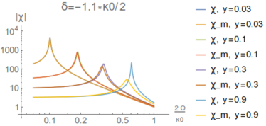
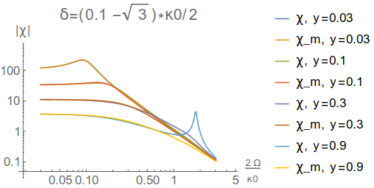
Figure 2: The plots of the susceptibilities $|\chi|$ and their approximations $|\chi_{m}|$ as function of frequency at detuning $\delta=-1.1\,\kappa_{0}/2$ (upper plot) and $(0.1-\sqrt{3})\,\kappa_{0}/2$ as function of frequency at the different power parameter $y$ (19c).

However, conditions (19a) are a result of the approximation. For accurate consideration we apply the Routh-Hurwitz criterion Routh (1877); Hurwitz (1895); Rabinovich and Trubetskov (1984); Gopal (2002) to investigate stability of the system, described by the susceptibility $\chi=m/(K-m\Omega^{2})$, and found that the accurate conditions of stability include (19a) plus one more condition on the pump

$$0<\Omega_{0}^{2}<\Omega_{0max}^{2},\quad \Omega_{0max}^{2}=\frac{\kappa_{0}}{|\delta|}\left(\delta^{2}-\left[\frac{\kappa_{0}}{2}\right]^{2}\right)$$ (19b)

$$\Omega_{0}^{2}=y\Omega_{0max}^{2},\quad 0<y<1$$ (19c)

Here $y$ is dimensionless power parameter.

Summing up, the rigidity based on dissipative coupling may be positive on both left and right slopes of the resonance curve, however, it is stable only on left one, $\delta<0$.

It is important that we can control characteristics of the stable rigidity. We can obtain approximation for eigenfrequency $\Omega_{m}$, relaxation rate $\delta_{m}$ and quality factor $Q_{m}$ of a mechanical oscillator created by the optical rigidity using the series (18) to demonstrate it:

$$\Omega_{m}^{2} =\frac{\Omega_{0}^{2}|\delta|\left(3\left[\frac{\kappa_{0}}{2}\right]^{2}-\delta^{2}\right)}{\left[\frac{\kappa_{0}}{2}\right]\left(\left[\frac{\kappa_{0}}{2}\right]^{2}+\delta^{2}\right)},$$ (20)

$$\delta_{m} =\frac{2\Omega_{0}^{2}|\delta|\left(\delta^{2}-\left[\frac{\kappa_{0}}{2}\right]^{2}\right)}{(\left[\frac{\kappa_{0}}{2}\right]^{2}+\delta^{2})^{2}},$$ (21)

$$Q_{m} \equiv\frac{\Omega_{m}}{2\delta_{m}}=\frac{\sqrt{3\left[\frac{\kappa_{0}}{2}\right]^{2}-\delta^{2}}\,(\left[\frac{\kappa_{0}}{2}\right]^{2}+\delta^{2})^{3/2}}{4\Omega_{0}\sqrt{|\delta|\left[\frac{\kappa_{0}}{2}\right]}(\delta^{2}-\left[\frac{\kappa_{0}}{2}\right]^{2})}$$ (22)

Here we assumed that $\delta<0$ for stability.

Although this consideration based on the series expansion is convenient, it is valid only for small frequency and small pump. It means that pump parameter $\Omega_{0}$ must be small. For large pump $\Omega_{0}$ we have to use the exact susceptibility $\chi$ instead of it’s approximation $\chi_{m}=m/(K_{m}-m\Omega^{2})$. On Fig. 2 we present the plots of $|\chi|$ and $|\chi_{m}|$, for the detunings $\delta$, corresponding to the stable rigidity (19a) and different $y$. We see that the approximation (18) gives correct results for small power parameter $y\leq 0.3$ whereas for $y>0.3$ approximation is not valid.

Plots on Fig. 2 also show that choosing detuning $\delta$ and power parameter $y$ one can obtain an overdamped mechanical oscillator or an oscillator with high quality factor. So the optical rigidity based on dissipative coupling provides a very promising possibility to create a mechanical system with the characteristics chosen on demand.

Introduction of the stable optical rigidity converts the free mass into the artificially created mechanical oscillator and it is interesting to estimate it’s noise. Fluctuation force (12) impacts on it, it’s power spectral density $S_{Ffl}$ is equal to

$$S_{Ffl} =2\hslash m\Omega_{0}^{2}\frac{\left(\left[\frac{\kappa_{0}}{2}\right]^{2}+\delta^{2}\right)}{\left[\frac{\kappa_{0}}{2}\right]^{2}}\times$$ (23)

$$\qquad\times\left\{\big{|}g_{-}+j_{-}\big{|}^{2}+\big{|}g_{+}-j_{+}\big{|}^{2}\right\}.$$

we used the definitions (17) and the formula (59) with the notations in Appendix B. This formula can be rewritten through $\Omega_{m}$ using (20).

Due to action of $F_{fl}$ in equilibrium the oscillator possesses mean fluctuation energy $\mathcal{E}_{m}=m\Omega_{m}^{2}\langle x^{2}\rangle$ which is convenient to characterize by mean quantum number $n_{eff}$:

$$\mathcal{E}=\hslash\Omega_{m}n_{eff}$$ (24)

The spectral density $S_{Ffl}$ practically does not depend on spectral frequency $\Omega$ and for high quality factor $Q_{m}$ (22) it can be considered as a constant (white noise, not depending on $Q_{m}$). Consequently, mean energy $\mathcal{E}_{m}$ should increase with increase of $Q_{m}$. For the particular case our estimate gives

$$n_{eff} \simeq 240,\quad\text{at}\ \delta=-0.55\,\kappa_{0},\ y=0.01.$$ (25a)

For these parameters

$$\Omega_{m}\simeq 0.029\,\kappa_{0},\ \kappa_{0}\simeq 32.37\,\Omega_{0},\ Q_{m}\simeq 14.5.$$ (25b)

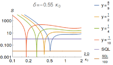
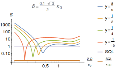
Figure 3: PSD $S_{\mathfrak{f}}$ as function of frequency $\Omega$ for amplitude detection ($\sin\theta=0$) with different power parameters $y$ (19c). On the top the detuning is $\delta=-5.5\,\kappa_{0}$, on the bottom — $\delta=\frac{0.1-\sqrt{3}}{2}\,\kappa_{0}$.

IV Detection of signal force

Using (7b, (13)) we obtain for the output amplitude in frequency domain:

$$a_{out} =\frac{\frac{\kappa_{0}}{2}+i\left[\delta+\Omega\right]}{\frac{\kappa_{0}}{2}-i\left[\delta+\Omega\right]}\,a_{in}+$$ (26)

$$+\frac{\eta\kappa_{0}A_{0}}{2}\cdot\frac{\frac{\kappa_{0}}{2}+i\delta}{\frac{\kappa_{0}}{2}-i\delta}\left(\frac{1}{\frac{\kappa_{0}}{2}+i\delta}-\frac{1}{\frac{\kappa_{0}}{2}-i(\delta+\Omega)}\right)\hat{x},$$

We have to substitute the mechanical displacement $\xi$ in frequency domain into (26) with account of the rigidity (16):

$$x =\frac{F_{fl}+F_{s}}{-m\Omega^{2}Q},\quad Q=1-\frac{K}{m\Omega^{2}}$$ (27)

and the fluctuation force $F_{fl}$ (see details in Appendix B).

We assume that the output wave is registered by a homodyne detector. Hence, we have to calculate the quadratures of the output wave. We define the amplitude quadrature $e_{a}$ andthe phase quadrature $e_{p}$ inthe output wave as following:

$$e_{a} =\frac{1}{\sqrt{2}}\left(\frac{\frac{\kappa_{0}}{2}-i\delta}{\frac{\kappa_{0}}{2}+i\delta}\,a_{out}+\frac{\frac{\kappa_{0}}{2}+i\delta}{\frac{\kappa_{0}}{2}-i\delta}\,a_{out-}^{\dagger}\right),$$ (28a)

$$e_{p} =\frac{1}{i\sqrt{2}}\left(\frac{\frac{\kappa_{0}}{2}-i\delta}{\frac{\kappa_{0}}{2}+i\delta}\,a_{out}-\frac{\frac{\kappa_{0}}{2}+i\delta}{\frac{\kappa_{0}}{2}-i\delta}\,a_{out-}^{\dagger}\right).$$ (28b)

The calculation of the output quadratures as the functions of the input amplitude ($a_{a}$) and phase ($a_{p}$) quadratures

$$a_{a} =\frac{a_{in}+a_{in-}^{\dagger}}{\sqrt{2}},\quad a_{p}=\frac{a_{in}-a_{in-}^{\dagger}}{i\sqrt{2}}$$ (29)

are presented in Appendix B, the results are:

$$e_{a} =E_{aa}a_{a}+E_{ap}a_{p}+\Phi_{a}f_{s},\quad f_{s}=\frac{F_{s}}{\sqrt{2\hslash m\Omega^{2}}}\,,$$ (30a)

$$e_{p} =E_{pa}a_{a}+E_{pp}a_{p}+\Phi_{p}f_{s},$$ (30b)

Here $f_{s}$ is a Fourier transform of the signal force normalized to the Standard Quantum Limit (SQL) for the free mass. The expressions for the coefficients in (30) are rather cumbersome and we present them using a consequence of notations in Appendix B.

In the homodyne detector we measure a quadrature $e_{\theta}=e_{a}\cos\theta+e_{p}\sin\theta$ in the output wave, where $\theta$ is a homodyne angle. Sensitivity is convenient to characterize by the quadrature $e_{\theta}$ recalculated to the SQL:

$$\mathfrak{f}_{\theta}=\frac{e_{a}\cos\theta+e_{p}\sin\theta}{\Phi_{a}\cos\theta+\Phi_{p}\sin\theta}$$ (31)

with the power spectral density (PSD)

$$S_{\mathfrak{f}}(\Omega) =S_{a}+S_{p},$$ (32)

$$S_{a} =\frac{\big{|}E_{aa}+E_{pa}\tan\theta\big{|}^{2}}{\big{|}\Phi_{a}+\Phi_{p}\tan\theta\big{|}^{2}},\quad S_{p}=\frac{\big{|}E_{ap}+E_{pp}\tan\theta\big{|}^{2}}{\big{|}\Phi_{a}+\Phi_{p}\tan\theta\big{|}^{2}}$$

Below we analyze sensitivity only for the stable rigidity (i.e. the conditions (19) are valid).

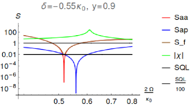
Figure 4: Amplitude detection. Presentation of the contributions by the different terms $S^{A}_{a}$ and $S^{A}_{p}$ (33) into the power spectral density $S_{\mathfrak{f}}$ for the particular power parameter $y=0.9$ and the detuning $\delta=-0.55\,\kappa_{0}$. The plot of the susceptibility $|\chi|$ is also presented.

IV.1 Amplitude detection

Amplitude detection is simpler to realize in experiment as compared with homodyne one. Formally it corresponds to $\sin\theta=0$ in the formulas (32):

$$S_{\mathfrak{f}}(\Omega) =S^{A}_{a}+S^{A}_{p},\quad S^{A}_{a}=\frac{\big{|}E_{aa}\big{|}^{2}}{\big{|}\Phi_{a}\big{|}^{2}},\ S^{A}_{p}=\frac{\big{|}E_{ap}\big{|}^{2}}{\big{|}\Phi_{a}\big{|}^{2}}$$ (33)

We obtain that even amplitude detection allows to surpass the SQL (i.e. $S_{\mathfrak{f}}<1$) by more than 100 times. Choosing the pump parameter $y$ one can vary both spectral frequency and range of the SQL surpassing — plots on Fig. 3 demonstrates it.

The top plots on Fig. 3 demonstrate the SQL overcoming by about 1000 times but in the narrow bandwidth. In contrast, the bottom plots demonstrate the more modest SQL overcoming by about 100 times but in the wider bandwidth. Note that the pump power on the top plots is about 10 times lesser than on the bottom ones (with the same pump parameter $y$).

Analysis shows that the SQL surpassing takes place when the coefficient $E_{aa}$ has minimum due to the compensation of the shot noise term $\sim\beta_{+}$ and the backaction term $\sim\Omega_{0}^{2}$ — see (61a) in Appendix B. The same compensation takes place for the coefficient $E_{ap}$ in (61c), but on slightly different spectral frequency $\Omega$.

For demonstration we present on Fig. 4 the contributions of the different terms $S^{A}_{a}$ and $S^{A}_{p}$ of the spectral density $S_{\mathfrak{f}}$ (33) for the particular pump parameter $y=0.9$ and the detuning $\delta=-0.55\,\kappa_{0}$. The plot of the susceptibility is also presented (it has different dimension) in order to show that the mentioned compensation takes place on frequencies different from frequency $\Omega_{m}$ of mechanical resonance.

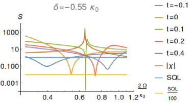
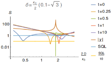
Figure 5: The PSD $S_{\mathfrak{f}}$ as a function of frequency $\Omega$ for homodyne detection with the constant power parameter $y=8/9$ (19c) at the different homodyne angles $t=\tan\theta$. On the top the detuning is $\delta=-5.5\,\kappa_{0}$, on the bottom — $\delta=\frac{0.1-\sqrt{3}}{2}\,\kappa_{0}$. The plot of the susceptibility $|\chi|$ is also presented.

IV.2 Homodyne detection

In this case we have the homodyne angle $\theta$ as an additional degree of freedom which provides a possibility to control the sensitivity. Indeed, even at the constant pump we can change the PSD by the tuning of the homodyne angle. As shown on Fig. 5 the PSD has a minimum at frequency $\Omega_{min}$ and it’s width $\Delta\Omega$ (where the SQL is surpassed, i.e. $S_{\mathfrak{f}}<1$) can be shifted and changed.

The plots on Fig. 5 demonstrate that frequency $\Omega_{min}$ grows with increase of the homodyne angle $\theta$, whereas the bandwidth $\Delta\Omega$ initially decreases until $\Omega_{min}<\Omega_{m}$ and increases when $\Omega_{min}>\Omega_{m}$. Note that if $\Omega_{min}\simeq\Omega_{m}$ we have the most strong minimum of the PSD but in the very narrow bandwidth.

Detailed analysis shows that for the particular plots on top of Fig. 5 the amplitude part $S_{a}$ makes the main contribution into the PSD (32). The minimum of the PSD (practically the minimum of $S_{a}$) takes place when the shot noise term $\sim(\beta_{+}-\beta_{-}^{*}\tan\theta)$ and the backaction noise term $\sim(E_{aa1}+E_{pa1}\tan\theta)$ compensate each others — for details see formulas (61) in Appendix B. The plot of the susceptibility is also presented (it has different dimension) in order to show that the mentioned compensation takes place on frequencies close to frequency $\Omega_{m}$ of the mechanical resonance.

V Model of Dissipative Coupling based on Michelson-Sagnac interferometer

For realization of dissipative coupling without dispersive one we consider a MSI first suggested in Xuereb et al. (2011). In the Fabry-Perot cavity, shown in Fig. 6, the MSI plays the role of the input generalized mirror (GM). Here we present the generalized model with the non-balanced beam splitter with amplitude transmittance $T_{bs}$ and reflectivity $R_{bs}$ and the partially reflecting mirror $M$ with transmittance $T$ and reflectivity $R$. We assume that the GM size is smaller than the distance $L$ between the not movable beam splitter and the end mirror so both amplitude transmittance $\mathbb{T}$ and reflectivity $\mathbb{R}$ of the GM depend on position $X$ of movable mirror $M$ with mass $m$ and do not depend on spectral frequency.

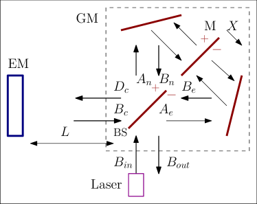
Figure 6: MSI with the input non-balanced beam splitter ($T_{bs}\neq R_{bs}$) and the movable partially reflective mirror $M$ with mass $m$. It plays the role of the input GM of the cavity pumped by the laser detuned from resonance.

We start from the boundary conditions on the beam splitter:

$$A_{e} =T_{bs}B_{c}-R_{bs}B_{in},\ A_{n}=R_{bs}B_{c}+T_{bs}B_{in},$$ (34a)

$$B_{out} =T_{bs}B_{n}-R_{bs}B_{e},\ D_{c}=T_{bs}B_{e}+R_{bs}B_{n},$$ (34b)

where $B_{in},\ B_{out},\ B_{c},\ D_{c},\ A_{e},\ A_{n},\ B_{e},\ B_{n}$ are the complex amplitudes of the incident and reflected waves on the beam splitter — see the notations on Fig. 6. The boundary conditions on the mirror M give

$$B_{e} =-RA_{e}e^{2ik\ell_{e}}+TA_{n}e^{ik(\ell_{e}+\ell_{n})},$$ (35a)

$$B_{n} =RA_{n}e^{2ik\ell_{n}}+TA_{e}e^{ik(\ell_{e}+\ell_{n})}$$ (35b)

where $k=\omega_{p}/c$ is a wave vector and $c$ is the speed of light, $k\ell_{e}$ ($k\ell_{n}$) is the accumulated phase of the light traveling between the beam splitter and the mirror $M$ through the east (north) arm.

We define reflectivity and transmittance of the GM as

$$D_{c} =\mathbb{T}B_{in}+\mathbb{R}_{\rhd}B_{c},\quad B_{out}=\mathbb{T}B_{c}+\mathbb{R}_{\lhd}B_{in}.$$ (36)

Using (34) and (35) one can derive

$$\mathbb{T} =e^{i\phi_{+}}\left\{2RR_{bs}T_{bs}\cos\phi_{-}-T\Delta_{bs}\right\},$$ (37a)

$$\mathbb{R}_{\rhd} =Re^{i\phi_{+}}\times$$ (37b)

$$\qquad\times\left\{\Delta_{bs}\cos\phi_{-}-i\sin\phi_{-}+\frac{2TT_{bs}R_{bs}}{R}\right\},$$

$$\mathbb{R}_{\lhd} =-Re^{i\phi_{+}}\times$$ (37c)

$$\qquad\times\left\{\Delta_{bs}\cos\phi_{-}+i\sin\phi_{-}+\frac{2TT_{bs}R_{bs}}{R}\right\},$$

$$\phi_{\pm}=k\big{(}\ell_{e}\pm\ell_{n}\big{)},\quad\Delta_{bs}=R_{bs}^{2}-T_{bs}^{2}$$ (37d)

It is obvious that the sum phase $\phi_{+}$ does not depend on the displacement $X$ of the mirror M, but the phase difference $\phi_{-}$ does depend. Below we present the displacement $X=x_{0}+x$ as a sum of the constant mean value $x_{0}$ and the small addition $x$ so that $\phi_{-}=\phi_{0}+2kx$ and expand reflectivity and transmittance of the GM in a series over $x$.

One can easy derive that for the realization of pure dissipative coupling (but not combination of dissipative and dispersive ones) we must have the relative derivatives of $\mathbb{T}$, $\mathbb{R}_{\rhd}$ and $\mathbb{R}_{\lhd}$ over $\phi_{-}$ to be real. Calculations give:

$$\frac{\partial_{\phi_{-}}\mathbb{T}}{\mathbb{T}} =\frac{-2RR_{bs}T_{bs}\sin\phi_{-}}{2RR_{bs}T_{bs}\cos\phi_{-}-T\Delta_{bs}},$$ (38a)

$$\frac{\partial_{\phi_{-}}\mathbb{R}_{\rhd}}{\mathbb{R}_{\rhd}} =\frac{-R\Delta_{bs}\sin\phi_{-}-iR\cos\phi_{-}}{R\Delta_{bs}\cos\phi_{-}-iR\sin\phi_{-}+2TT_{bs}R_{bs}}.$$ (38b)

We see that the relative derivative (38a) is real at any combination of the parameters. In order to have the real derivative (38b) we have two possibilities:

a) the balanced beam splitter ($\Delta_{bs}=0$) and the perfectly reflective mirror M ($T=0$); this case was analyzed in Xuereb et al. (2011); S.P. Vyatchanin and A.B. Matsko (2016);

b) the non-balanced beam splitter and the partially transparent mirror M ($T\neq 0$) — in this case we have to choose $\phi_{-}=\phi_{0}$, where $\phi_{0}$ is the solution of equation

$$\cos\phi_{0} =\frac{-R\Delta_{bs}}{2TT_{bs}R_{bs}},$$ (38c)

$$\mathbb{T}_{0}=\mathbb{T}|_{\phi_{-}=\phi_{0}} =-e^{i\phi_{+}}\frac{\Delta_{bs}}{T},$$ (38d)

$$|\mathbb{R}_{0}|=|\mathbb{R}_{\rhd}|_{\phi_{-}=\phi_{0}} =\frac{\sqrt{(2T_{bs}R_{bs})^{2}-R^{2}}}{T},$$ (38e)

$$\left.\frac{\partial_{\phi_{-}}\mathbb{T}}{\mathbb{T}}\right|_{\phi_{-}=\phi_{0}} =\frac{2RTR_{bs}T_{bs}\sin\phi_{0}}{\Delta_{bs}}=\frac{R|\mathbb{R}_{0}|}{|\mathbb{T}_{0}|}.$$ (38f)

The cavity should have high finesse. Hence, for $|\mathbb{T}_{0}|\ll 1$ one have to have $|\Delta_{bs}|\ll T$. So assuming $e^{i\phi_{+}}=-1$ we obtain in first order approximation over $x$

$$\mathbb{T} =\mathbb{T}_{0}\left(1+\frac{R|\mathbb{R}_{0}|}{|\mathbb{T}_{0}|}\,2kx+\dots\right),$$ (39)

$$\mathbb{R}_{\rhd} =\mathbb{R}_{0}\left(1-\frac{R|\mathbb{T}_{0}|}{|\mathbb{R}_{0}|}\,2kx+\dots\right).$$ (40)

We see that for the realization of dissipative coupling with the partially transparent mirror M we should choose the correct angle $\phi_{0}$) (i.e. the constant displacement $x_{0}$). It is important that we can choose the parameters of the GM on demand by variation of the beam splitter parameters $(R_{bs},\ T_{bs})$.

The small displacement $x$ of the mirror $M$ from the mean position $x_{0}$ provides modulation of the relaxation rate of the Fabry-Perot interferometer:

$$\kappa =\kappa_{0}(1+\eta x),\quad\kappa_{0}=\frac{|\mathbb{T}|^{2}}{\tau},\quad\tau=\frac{2L}{c}$$ (41a)

$$\eta =4k\frac{R|\mathbb{R}_{0}|}{|\mathbb{T}_{0}|}\,.$$ (41b)

It is easy to demonstrate that all equations for this optomechanical system are the same as derived in Sec. II.

It is important that on the example of the considered interferometer as the GM we can demonstrate the peculiar property of a light pressure force in an optomechanical system with dissipative coupling. Indeed, using the notations on Fig. 6 we can write a ponderomotive force acting on the mirror M:

$$F= 2\hslash kR^{2}\big{(}|A_{n}|^{2}-|A_{e}|^{2}\big{)}=$$ (42)

$$=4\hslash kR^{2}\left(B_{c}B_{in}^{*}+B_{c}^{*}B_{in}\right).$$ (43)

Here in the last equation we used the input-output relation (34) putting $R_{bs}=T_{bs}$. Recall that for dispersive coupling the ponderomotive force is just proportional to the square of the amplitude of the intracavity wave. In contrast, for the optomechanical system with dissipative coupling the force is proportional to the cross product of the incident $B_{in}$ and the inside $B_{c}$ amplitudes as it follows from (42). The light pressure force depends on phase difference between $B_{in}$ and $\tilde{B}_{c}$, so it can be also called as the interferometric pressure. It is precisely this property provides the additional possibilities for the realization of the stable rigidity. We would like to pay attention on resemblance between formulas (42) and (12), obtained in frame of the Hamiltonian approach.

Note that the realization of the stable optical rigidity was proposed Tarabrin et al. (2013) and elegantly demonstrated Sawadsky et al. (2015); Cripe et al. (2018) for a similar scheme with alone MSI presented on Fig. 6, without any cavity and without focusing attention on dissipative or dispersive coupling is used. In contrast, in the scheme analyzed in this paper the stable optical rigidity is a property of cavity with dissipative coupling and we formulated the conditions when MSI is a generalized mirror with dissipative coupling (but not a combination of dissipative and dispersive ones).

Conclusion

We analyzed the optical rigidity based on dissipative coupling and formulated the conditions (19) of the stable optical rigidity. Recall that using dispersive coupling one can get only the unstable rigidity V.B. Braginsky and F.Ya. Khalili (1999); F.Ya. Khalili (2001).

The rigidity based on dissipative coupling may be positive on the both left and right slopes of the resonance curve (but stable only on the left one, $\delta<0$), whereas the positive (unstable) rigidity in case of dispersive coupling takes place on the right slope only.

We show that physical reason of stability of the rigidity based on dissipative coupling is interference between the input and intracavity waves, originating the more complicated dependence of the light pressure force as compared with dispersive coupling.

We have shown that dissipative coupling can be realized in the MSI with the partially transparent mirror M — it is the generalization of the previous results Xuereb et al. (2011); S.P. Vyatchanin and A.B. Matsko (2016) for the perfectly reflecting mirror M. It provides the possibility to use a thin membrane Arcizet et al. (2006); Zwickl et al. (2008); Borkje et al. (2010) as the mirror M with extra small mass $m$ for the experimental realization.

For the estimation we assume:

$$m =10^{-8}\,\text{g},\quad k=\frac{2\pi}{\lambda},\quad\lambda=10^{-6}\,\text{m},$$ (44a)

$$W_{in}=10^{-4}\,\text{W},\quad R^{2}=0.7,\quad|\mathbb{T}|^{2}=10^{-4}$$ (44b)

Using (17), (20) we obtain the estimations of the power parameter $\Omega_{0}$ and the mechanical eigenfrequency $\Omega_{m}$:

$$\Omega_{0} =\sqrt{\frac{4kW_{in}}{mc|\mathbb{T}|^{2}}}\simeq 92\cdot 10^{3}\,\text{rad/s},$$ (45a)

$$\Omega_{m} \simeq 86\cdot 10^{3}\,\text{rad/s}.$$ (45b)

In the last estimation we put $\delta=-0.55\,\kappa_{0}$.

It means the possibility to create a mechanical nano-oscillator with the eigenfrequency in the range of hundreds kHz from a free mass and the stable optical rigidity. The fluctuation light pressure force is a source of the excitation of the oscillator, we show that in equilibrium the mean quantum number $n_{eff}$ of such oscillator may be about $200$. This estimate corresponds to coherent pump, however, for specially tuned squeezed pump mean quantum number $n_{eff}$ can be smaller.

Appendix A Dissipation Description

In this Appendix we present the detailed description of the Hamiltonian (1) and the derivation of the equations (2) for the field $\hat{a}_{c}$ inside cavity and the mechanical coordinate $\hat{x}$.

We write the Hamiltonians $H_{T},\ H_{\kappa}$ in form

$$H_{\kappa} =-i\hslash\sqrt{\frac{\kappa\,\Delta\omega}{2\pi}}\,\sum_{q=1}^{\infty}\left(\hat{a}_{c}^{\dagger}\hat{b}_{q}-\hat{b}_{q}^{\dagger}\hat{a}_{c}\right)\,,$$ (46)

$$H_{T} =\sum_{q=1}^{\infty}\hslash\omega_{q}\,\hat{b}_{q}^{\dagger}\hat{b}_{q}\,,$$ (47)

Here we present a thermal bath as infinite number of the oscillators with the annihilation and creation operators $\hat{b}_{q},\ \hat{b}_{q}^{\dagger}$, $q$ is integer number, frequencies $\omega_{q}$ of these oscillators are separated by $\Delta\omega=\omega_{q}-\omega_{q-1}$, we hold in mind that below we put

$$\Delta\omega\to 0$$ (48)

The commutators and correlators are

$$\big{[}\hat{b}_{q},\hat{b}_{q^{\prime}}^{\dagger}\big{]}=\delta_{qq^{\prime}},\quad\big{\langle}\hat{b}_{q}\hat{b}_{q^{\prime}}^{\dagger}\big{\rangle}=\,\delta_{qq^{\prime}}\,.$$ (49)

(The temperature of the bath is assumed to be zero.) We write down the movement equations:

$$\dot{\hat{a}}_{c} =\frac{1}{i\hslash}\big{[}\hat{a}_{c},H\big{]}=-i\omega_{0}\hat{a}_{c}-\sqrt{\frac{\kappa\,\Delta\omega}{2\pi}}\sum_{q=1}^{\infty}\hat{b}_{q},$$ (50a)

$$\dot{\hat{b}}_{q} =-i\omega_{q}\hat{b}_{q}+\sqrt{\frac{\kappa\,\Delta\omega}{2\pi}}\hat{a}_{c}.$$ (50b)

Introducing the slow amplitudes

$$\hat{a}_{c} =\hat{a}e^{-i\omega_{p}t},\quad\hat{b}_{q}\Rightarrow\hat{b}_{q}e^{-i\omega_{q}t}$$ (50c)

we get

$$\dot{\hat{a}}(t)-i\delta\,\hat{a} =-\sqrt{\frac{\kappa\,\Delta\omega}{2\pi}}\sum_{q=1}^{\infty}\hat{b}_{q}e^{i(\omega_{p}-\omega_{q})t},$$ (50d)

$$\dot{\hat{b}}_{q} =\sqrt{\frac{\kappa\,\Delta\omega}{2\pi}}\,\hat{a}e^{-i(\omega_{p}-\omega_{q})t}.$$ (50e)

We substitute the formal solution of (50e) for $\dot{\hat{b}}_{q}$ into (50d) using method of successive approximations based on (48):

$$\hat{b}_{q} =\hat{b}_{q}(0)+\sqrt{\frac{\kappa\,\Delta\omega}{2\pi}}\int\limits_{0}^{t}\hat{a}_{c}(t^{\prime})e^{-i(\omega_{p}-\omega_{q})t^{\prime}}\,dt^{\prime},$$ (51a)

$$\dot{\hat{a}} -i\delta\,\hat{a}=-\sum_{q=1}^{\infty}\left(\sqrt{\frac{\kappa\,\Delta\omega}{2\pi}}\,\hat{b}_{q}(0)e^{i(\omega_{p}-\omega_{q})t}-\right.$$ (51b)

$$\quad\left.-\frac{\kappa\,\Delta\omega}{2\pi}\,\int\limits_{0}^{t}\hat{a}_{c}(t^{\prime})\,e^{i(\omega_{p}-\omega_{q})(t-t^{\prime})}\,dt^{\prime}\right)=$$ (51c)

$$=\sqrt{\kappa}\,\hat{a}_{in}-\frac{\kappa}{2}\,\hat{a}\,.$$ (51d)

Below we present the details of the derivation (51d).

In the further calculations in the limit (48) we replace the sum by the integral using the rule

$$\Delta\omega\sum_{q=1}^{\infty}\Rightarrow\int\limits_{0}^{\infty}d\omega_{q}\,.$$ (52)

Using (49) we calculate the commutator (3) for $a_{in}$ defined in (51b)

$$\hat{a}_{in}(t) \equiv\sqrt{\frac{\Delta\omega}{2\pi}}\sum_{q=1}^{\infty}\hat{b}_{q}(0)e^{i(\omega_{p}-\omega_{q})t},$$ (53a)

$$\big{[}\hat{a}_{in}(t),\hat{a}_{in}^{\dagger}(t^{\prime})\big{]} \equiv\frac{\Delta\omega}{2\pi}\sum_{q=1}^{\infty}e^{i(\omega_{p}-\omega_{q})(t-t^{\prime})}=$$ (53b)

$$=\delta(t-t^{\prime})\,,$$ (53c)

Here $$\delta(t)$$ is the Dirac delta function. By the similar calculation we obtain the correlator (4) assuming that the thermostat oscillators are in the main state:

$$\left\langle b_{q}b_{q^{\prime}}^{\dagger}\right\rangle =\delta_{kk^{\prime}},\quad\left\langle b_{q}^{\dagger}b_{q^{\prime}}\right\rangle=0$$ (53d)

where $$\delta_{kk^{\prime}}$$ is the Kronecker delta.

We calculate the term (51c) using the rule (52):

$$\int\limits_{0}^{t}\hat{a}_{c}(t^{\prime})\left[\sum_{q=1}^{\infty}\frac{\kappa\,\Delta\omega}{2\pi}\,e^{i(\omega_{p}-\omega_{q})(t-t^{\prime})}\right]dt^{\prime}=$$ (53e)

$$=\int\limits_{0}^{t}\hat{a}_{c}(t^{\prime})\,\frac{\kappa}{2\pi}\left[\int\limits_{0}^{\infty}\,e^{i(\omega_{p}-\omega_{q})(t-t^{\prime})}d\omega_{q}\right]dt^{\prime}=$$ (53f)

$$\qquad=\frac{\kappa}{2\pi}\,\int\limits_{0}^{t}\hat{a}_{c}(t^{\prime})\,2\pi\,\delta(t-t^{\prime})dt^{\prime}=\frac{\kappa}{2}\,\hat{a}_{c}(t)\,.$$ (53g)

From (46) we get for the mechanical coordinate using the definition (2c)

$$\ddot{\hat{x}} =\frac{i\hslash\eta}{2m}\sqrt{\frac{\kappa_{0}\,\Delta\omega}{2\pi}}\,\sum_{q=1}^{\infty}\left(\hat{a}_{c}^{\dagger}\hat{b}_{q}-\hat{b}_{q}^{\dagger}\hat{a}_{c}\right)+\frac{F_{s}}{m}.$$ (54)

Using the definition (53a) we obtain (2b).

Appendix B Calculations of the output quadratures

Here we present the details of calculations for the output quadratures. Here we use the following notations in order to compact the formulas below:

$$\psi =\frac{\kappa_{0}}{2}-i\delta,\quad\psi^{*}=\frac{\kappa_{0}}{2}+i\delta,$$ (55a)

$$\Psi =\frac{\kappa_{0}}{2}-i\delta-i\Omega,\quad\Psi^{*}=\frac{\kappa_{0}}{2}+i\delta+i\Omega,$$ (55b)

$$\Psi_{-} =\frac{\kappa_{0}}{2}-i\delta+i\Omega,\quad\Psi^{*}_{-}=\frac{\kappa_{0}}{2}+i\delta-i\Omega\,,$$ (55c)

For the fluctuation part of the light pressure force $F_{fl}$ in frequency domain we get using (12) and the notations (14):

$$F_{fl} =\frac{i\hslash A_{0}\eta\sqrt{\kappa}_{0}}{2}\left\{\frac{a_{in-}^{\dagger}}{\psi}-\frac{a_{in}}{\psi^{*}}-\frac{a_{in-}^{\dagger}}{\Psi^{*}_{-}}+\frac{a_{in}}{\Psi}\right\},$$ (56)

$$g_{+} \equiv\frac{\kappa_{0}}{4}\left(\frac{1}{\psi}+\frac{1}{\psi^{*}}\right),\quad g_{-}\equiv\frac{\kappa_{0}}{4i}\left(\frac{1}{\psi}-\frac{1}{\psi^{*}}\right)\,,$$ (57)

$$j_{+} \equiv\frac{\kappa_{0}}{4}\left(\frac{1}{\Psi}+\frac{1}{\Psi_{-}^{*}}\right)\,,\quad j_{-}\equiv\frac{\kappa_{0}}{4i}\left(\frac{1}{\Psi}-\frac{1}{\Psi_{-}^{*}}\right).$$ (58)

and express it through the quadratures (29) of the input wave

$$F_{fl} =\sqrt{2}\hslash A_{0}\eta\left\{-a_{a}\big{(}g_{-}+j_{-}\big{)}+a_{p}\big{(}g_{+}-j_{+}\big{)}\right\}$$ (59)

Substituting it into (27) and then into (26) using (29) we obtain:

$$a_{out} =\frac{\Psi^{*}}{\Psi}\,a_{in}+\frac{\eta\kappa_{0}A_{0}}{2}\cdot\frac{\psi^{*}}{\psi}\left(\frac{1}{\psi^{*}}-\frac{1}{\Psi}\right)\times$$ (60)

$$\quad\times\frac{\sqrt{2}\hslash A_{0}\eta}{-m\Omega^{2}Q}\left\{-a_{a}\big{(}g_{-}+j_{-}\big{)}+a_{p}\big{(}g_{+}-j_{+}\big{)}\right\}.$$

Then we substitute it into the definitions (28) and after simple but awkward calculations we finally obtain the coefficients in (30):

$$E_{aa} =\beta_{+}+E_{aa1},$$ (61a)

$$E_{aa1}=\frac{2\Omega_{0}^{2}}{\Omega^{2}Q}\left(g_{+}-j_{+}\right)\big{(}g_{-}+j_{-}\big{)},$$ (61b)

$$E_{ap} =-\beta_{-}^{*}+E_{ap1},$$ (61c)

$$E_{ap1}=\frac{2\Omega_{0}^{2}}{\left(\Omega^{2}Q\right)}\left(-g_{+}+j_{+}\right)\big{(}g_{+}-j_{+}\big{)},$$ (61d)

$$\Phi_{a} =\sqrt{\frac{4\Omega_{0}^{2}}{\Omega^{2}}}\left(\frac{-g_{+}+j_{+}}{Q}\right),$$ (61e)

$$E_{pa} =\beta_{-}^{*}-E_{pa1},$$ (61f)

$$E_{pa1}=\frac{2\Omega_{0}^{2}}{\Omega^{2}Q}\left(g_{-}+j_{-}\right)\big{(}g_{-}+j_{-}\big{)},$$ (61g)

$$E_{pp} =\beta_{+}+E_{pp1},$$ (61h)

$$E_{pp1}=\frac{2\Omega_{0}^{2}}{\Omega^{2}Q}\left(g_{-}+j_{-}\right)\big{(}g_{+}-j_{+}\big{)},$$ (61i)

$$\Phi_{p} =\sqrt{\frac{4\Omega_{0}^{2}}{\Omega^{2}}}\left(\frac{g_{-}+j_{-}}{Q}\right).$$ (61j)

where

$$\beta_{+} =\frac{1}{2}\left(\frac{\psi\Psi^{*}}{\psi^{*}\Psi}+\frac{\psi^{*}\Psi_{-}}{\psi\Psi_{-}^{*}}\right),$$ (62a)

$$\beta_{-} =\frac{1}{2i}\left(\frac{\psi\Psi^{*}}{\psi^{*}\Psi}-\frac{\psi^{*}\Psi_{-}}{\psi\Psi_{-}^{*}}\right)$$ (62b)

and $\Omega_{0}^{2}$ is the normalized pump (17).

References

- Aspelmeyer et al. (2014) M. Aspelmeyer, T. Kippenber, and F. Marquardt, Reviews of Modern Physics 86, 1391–1452 (2014).
- Povinelli et al. (2005) M. L. Povinelli, M. Lončar, M. Ibanescu, E. J. Smythe, S. G. Johnson, F. Capasso, and J. D. Joannopoulos, Opt. Lett. 30, 3042–3044 (2005), URL http://ol.osa.org/abstract.cfm?URI=ol-30-22-3042.
- Maslov et al. (2013) A. V. Maslov, V. N. Astratov, and M. I. Bakunov, Phys. Rev. A 87, 053848 (2013), URL http://link.aps.org/doi/10.1103/PhysRevA.87.053848.
- S.P. Vyatchanin and A.B. Matsko (1993) S.P. Vyatchanin and A.B. Matsko, Sov.Phys – JETP 77, 218–221 (1993).
- S.P. Vyatchanin and A.B. Matsko (1996) S.P. Vyatchanin and A.B. Matsko, Sov. Phys. – JETP 82, 107 (1996).
- A.B. Matsko and S.P. Vyatchanin (1997) A.B. Matsko and S.P. Vyatchanin, Applied Physics B 64, 167–171 (1997), ISSN 1432-0649, URL http://dx.doi.org/10.1007/s003400050161.
- H.J. Kimble et al. (2001) H.J. Kimble, Y. Levin, A.B. Matsko, K.S. Thorne, and S.P. Vyatchanin, Phys. Rev. D 65, 022002 (2001), eprint arXiv:gr-qc/0008026v2.
- V.B. Braginsky and F.Ya. Khalili. (1990) V.B. Braginsky and F.Ya. Khalili., Physics Letters A 147, 251–256 (1990).
- V.B. Braginsky et al. (2000) V.B. Braginsky, M.L. Gorodetsky, F.Y. Khalili, and K.S. Thorne, Physical Review D 61, 044002 (2000).
- LVC-Collaboration (2013) LVC-Collaboration, arXiv 1304.0670 (2013).
- Aso et al. (2013) Y. Aso et al., Phys. Rev. D 88, 043007 (2013).
- Dooley et al. (2014) K. Dooley, T. Akutsu, S. Dwyer, and P. Puppo, arXiv 1411.6068 (2014).
- C.Affeld et al. (2104) C.Affeld, K. Danzmann, K. Dooley, H. Grote, M. Hewitson, S. Hild, J. Hough, J. Leong, H. Luck, and M. Prijatelj, Classical and Quantum Gravity 32, 224002 (2104).
- J. Aasi et al et al.(2015) (LIGO Scientific Collaboration) J. Aasi et al (LIGO Scientific Collaboration) et al., Classical and Quantum Gravity 32, 074001 (2015).
- F. Acernese et al, (2015) (Virgo Collaboration) F. Acernese et al, (Virgo Collaboration), Classiacal and Quantum Gravity 32, 024001 (2015).
- B.P. Abbott et al, (2018) (LIGO Scientific Collaboration, Virgo Collaboration and KAGRA Collaboration) B.P. Abbott et al, (LIGO Scientific Collaboration, Virgo Collaboration and KAGRA Collaboration), Living Reviews in Relativity 21, 3 (2018).
- B. P. Abbott et al, (2016) (LIGO Scientific Collaboration and Virgo Collaboration) B. P. Abbott et al, (LIGO Scientific Collaboration and Virgo Collaboration), Phys. Rev. Lett. 116, 241103 (2016).
- B.P. Abbott et al, (2017a) (LIGO Scientific Collaboration and Virgo Collaboration) B.P. Abbott et al, (LIGO Scientific Collaboration and Virgo Collaboration), Phys. Rev. Lett. 119, 161101 (2017a).
- B.P. Abbott et al, (2017b) (LIGO Scientific Collaboration and Virgo Collaboration) B.P. Abbott et al, (LIGO Scientific Collaboration and Virgo Collaboration), Phys. Rev. Lett. 119, 141101 (2017b).
- F. Acernese et al (2018) (Virgo Collaboration) F. Acernese et al (Virgo Collaboration), arXiv 1807.03275 (2018).
- M. Wu et al. (2014) M. Wu, A.C. Hryciw, C. Healey, D.P. Lake, H. Jayakumar, M.R. Freeman, J.P. Davis, and P.E. Barclay, Physical Review X 4, 021052 (2014).
- S. Forstner and S. Prams and J. Knittel and E.D. van Ooijen and J.D. Swaim and G.I. Harris and A. Szorkovszky and W.P. Bowen and H. Rubinsztein-Dunlop (2012) S. Forstner and S. Prams and J. Knittel and E.D. van Ooijen and J.D. Swaim and G.I. Harris and A. Szorkovszky and W.P. Bowen and H. Rubinsztein-Dunlop, Physical Review Letters 108, 120801 (2012).
- V.B. Braginsky (1968) V.B. Braginsky, Sov. Phys. JETP 26, 831–834 (1968).
- V.B. Braginsky and F.Ya. Khalili (1992) V.B. Braginsky and F.Ya. Khalili, Quantum Measurement (Cambridge University Press, Cambridge, 1992).
- Kippenberg and Vahala (2008) T. Kippenberg and K. Vahala, Science 321, 1172–1176 (2008).
- J.M. Dobrindt and T.J. Kippenberg (2010) J.M. Dobrindt and T.J. Kippenberg, Physical Review Letters 104, 033901 (2010).
- Vyatchanin and Zubova (1995) S. Vyatchanin and E. Zubova, Physics Letters A 201, 269–274 (1995).
- V.B. Braginsky and F.Ya. Khalili (1999) V.B. Braginsky and F.Ya. Khalili, Phys. Lett. A 257, 241 (1999).
- F.Ya. Khalili (2001) F.Ya. Khalili, Physics Letters A 288, 251–256 (2001), eprint arXiv:gr-qc/0107084.
- S.P. Vyatchanin and A.B. Matsko (2016) S.P. Vyatchanin and A.B. Matsko, Physical Review A 93, 063817 (2016).
- F. Elste and S.M. Girvin and A.A. Clerk (2009) F. Elste and S.M. Girvin and A.A. Clerk, Physical Review Letters 102, 207209 (2009).
- M. Li and W.H.P. Pernice and H.X. Tang (2009) M. Li and W.H.P. Pernice and H.X. Tang, Physical Review Letters 103, 223901 (2009).
- Hryciw et al. (2015) A. Hryciw, M. Wu, B. Khanaliloo, and P. Barclay, Optica 2, 491 (2015).
- Sawadsky et al. (2015) A. Sawadsky, H. Kaufer, R. Nia, S. Tarabrin, F. Khalili, K. Hammerer, and R. Schnabel, Physical Review Letters 114, 043601 (2015).
- A. Kronwald and F. Marquardt and A.A. Clerk (2013) A. Kronwald and F. Marquardt and A.A. Clerk, Physical Review A 88, 063833 (2013).
- Tan et al. (2013) H. Tan, G. Li, and P. Meystre, Physical Revbiew A 87, 033829 (2013).
- Zhu et al. (2014) J. Zhu, H.Huang, and G. Li, Journal of Applied Physics 115, 033102 (2014).
- K. Qu and G.S. Agarwal (2015) K. Qu and G.S. Agarwal, Physical Review A 91, 063815 (2015).
- W.G. Gu and G.X. Li and Y.P. Yang (2013) W.G. Gu and G.X. Li and Y.P. Yang, Physical Review A 88, 013835 (2013).
- Gu and Li (2013) W. Gu and G. Li, Optics Express 21, 20423 (2013).
- S. Huang and G.S. Agarwal (2010a) S. Huang and G.S. Agarwal, Physical Review A 81, 053810 (2010a).
- S. Huang and G.S. Agarwal (2010b) S. Huang and G.S. Agarwal, Physical Review A 82, 033811 (2010b).
- Weiss et al. (2013) T. Weiss, C. Bruder, and A. Nunnenkamp, New Journal of Physics 15, 045017 (2013).
- Xuereb et al. (2011) A. Xuereb, R. Schnabel, and K. Hammerer, Physical Review Letters 107, 213604 (2011).
- Tarabrin et al. (2013) S. Tarabrin, H. Kaufer, F. Khalili, R. Schnabel, and K. Hammerer, Physical Review A 88, 023809 (2013).
- A.A. Clerk and M.H. Devoret and S.M. Girvin and F. Marquardt and R.J. Schoelkopf (2010) A.A. Clerk and M.H. Devoret and S.M. Girvin and F. Marquardt and R.J. Schoelkopf, Reviews of Modern Physics 82, 1155 (2010), eprint arXiv:08104729.
- Marquardt and Girvin (2009) F. Marquardt and S. Girvin, Physics 2, 40 (2009).
- V.B.Braginsky, I.I.Minakova (1964) V.B.Braginsky, I.I.Minakova, Vestnik Moskovskogo Universiteta, Seriya 3 p. 69 (1964), in Russian.
- Routh (1877) E. Routh, A Treatise on the Stability of a Given State of Motion: Particularly Steady Motion (Macmillan, 1877).
- Hurwitz (1895) A. Hurwitz, Math. Ann. 46, 273–284 (1895).
- Rabinovich and Trubetskov (1984) M. Rabinovich and D. Trubetskov, Introduction into Theory of Oscillations and Waves (in Russian) (Nauka, Moscow, 1984).
- Gopal (2002) M. Gopal, Control Systems: Principles and Design (Tata McGraw-Hill Education, 2002), 2nd ed.
- Cripe et al. (2018) J. Cripe, B. Danz, B. Lane, M. Lorio, J. Falcone, G. Cole, and T. Corbitt, Optics Lettes 43, 2193 (2018).
- Arcizet et al. (2006) O. Arcizet, P.-F. Cohadon, T. Briant, M. Pinard, A. Heidmann, J.-M. Mackowsk, C. Michel, L. Pinard, O. Francais, and L. Rousseau, Physical Review Letters 97, 133601 (2006).
- Zwickl et al. (2008) B. M. Zwickl, W. E. Shanks, A. M. Jayich, C. Yang, A. C. B. Jayich, J. D. Thompson, and J. G. E. Harris, Applied Physics Letters A 92, 103125 (2008).
- Borkje et al. (2010) K. Borkje, A. Nunnenkamp, B. Zwickl, C. Yang, J. Harris, and S. Girvin, Physical Review A 82, 013818 (2010).