Spin blockades to relaxation of hot multi-excitons in nanocrystals

Abstract

The rates of elementary photophysical processes in nanocrystals, such as carrier cooling, multiexciton generation, Auger recombination etc., are determined by monitoring the transient occupation of the lowest exciton band. The underlying assumption is that hot carriers relax rapidly to their lowest quantum level. Using femtosecond transient absorption spectroscopy in CdSe/CdS nanodots we challenge this assumption. Results show, that in nanodots containing a preexisting cold “spectator exciton”, only half of the photoexcited electrons relax directly to the band-edge and the rest are blocked in an excited state due to Pauli exclusion. Full relaxation occurs only after ~15 ps, as the blocked electrons flip spin. This requires review of numerous studies unaware of this ubiquitous and novel effect, which may facilitate hot carrier energy utilization as well.

I Introduction

Understanding how excess photon energy is dissipated after nanocrystal (NC) photoexcitation is essential for utilizing this energy in nanodot based solar cells or photo-detectors (König et al., 2010; Pandey and Guyot-Sionnest, 2009; Saeed et al., 2014; Konstantatos and Sargent, 2013; Williams et al., 2013; Li et al., 2017). Decades of ultrafast investigation show that inter-band photoexcitation of quantum dots is followed by rapid relaxation of hot carriers to the quantized band edge (BE) states within one or two picoseconds(Woggon et al., 1996; Nozik, 2001; Guyot-Sionnest et al., 1999; Klimov et al., 1999; Klimov, 2000; Sewall et al., 2006; Kambhampati, 2011; Cooney et al., 2007; Gdor et al., 2012, 2013; Spoor et al., 2015, 2017). Due to the large oscillator strength and low degeneracy of the BE exciton transition, evolution in its intensity and spectrum have played a pivotal part in probing quantum dot exciton cooling. These allegedly start with bi-exciton spectral shifts while carriers are hot, changing to a photoinduced bleach (PIB) due to state filling once the exciton relaxes. Accordingly, kinetics of this PIB buildup has served to characterize the final stages of carrier cooling (Klimov et al., 1999), and its amplitude per cold exciton provides a measure of underlying state degeneracy (Efros and Efros, 1982; Esch et al., 1990).

Hot multi-excitons (MX), generated for instance through sequential multi-photon absorption of femtosecond pulses, (Klimov, 2007; Kambhampati, 2012), add a new relaxation process to this scenario (Klimov et al., 2000). Auger recombination (AR) reduces an N exciton state to N-1 plus heat, initially deposited in the remaining carriers and later transferred to the lattice. Depending on N, this shortens the lifetime of MXs relative to a single exciton by two to three orders of magnitude. Again, investigation of AR dynamics is based on the amplitude and decay kinetics of the BE bleach with interpretation based on the following assumptions: 1) that ultrafast cooling of hot excitons leads directly to occupation of the lowest electron and hole states (in accordance with the lattice temperature and the state degeneracy), and 2) that aside from mild spectral shifts induced in the remaining band edge transitions, after carrier cooling is over the BE PIB increases linearly with N until the BE states are full (again dictated by state degeneracy).

To test these assumptions, three pulse saturate-pump-probe experiments were conducted in our lab, measuring fs transient absorption (TA) of PbSe NCs in the presence and absence of single cold spectator excitons (Gdor et al., 2015). This method hinges on the separation of timescales between AR and radiative recombination, the latter being much slower. Given the vast absorption cross sections of NCs, (Leatherdale et al., 2002; Osborne et al., 2004; Jasieniak et al., 2009) it is easy to excite nearly all particles in a sample with at least one photon even with ultrashort pulses. The rapid ensuing AR leads to a uniform population of NCs, all populated with a single cold exciton, within a fraction of a nanosecond. One can then probe the effect of a second exciton by comparing equivalent ultrafast pump-probe experiments in the samples with or without spectator excitons. Surprisingly, the BE bleach induced by a single relaxed exciton was found to be significantly larger than that induced by a second exciton which was added by above BE photoexcitation and left to cool down for 1-2 ps (Gdor et al., 2015). This finding was also shown to be consistent with the fluence dependent BE PIB saturation when exciting well above the optical band gap (BG) via comparison with simulations.

To unveil the cause of this discrepancy, the same approach is applied here to MXs in CdSe nanocrystals. This serves to test the generality of the results in lead salt. Due to the reduced band edge electron state degeneracy, each exciton has a much larger effect on the BE PIB in CdSe NCs, which simplifies analysis and assignment. Numerous investigations of CdSe NC photophysics have established: 1) that the BE exciton absorption is practically insensitive to hole state occupancy, allegedly due to the high density of valence bands in this material,(Klimov et al., 1999; Sewall et al., 2006) 2) that the BE transition in CdSe NCs reflects only a two-fold spin related degeneracy in the electron states (Efros and Rosen, 2000). Accordingly one relaxed exciton should bleach one-half of the initial BE absorption band, and the second erase it entirely. 3) that the much higher effective heavy hole mass in CdSe and involvement in spin-orbit coupling leads to much faster cooling of holes (<psec) relative to electrons (Klimov et al., 1999). Furthermore, the rapid electron relaxation measured in CdSe NCs is assigned to Auger cooling where excess electron energy transfers to the hole, and is then degraded to phonons (Klimov et al., 1999; Hendry et al., 2006; Cooney et al., 2007).

Contrary to the assumptions outlined above, our results show that adding a hot exciton to a relaxed singly occupied CdSe NC bleaches only half of the remaining BE absorption once the initial carrier cooling is over. It is further demonstrated that incomplete bleaching by the second exciton is due to hitherto unrecognized random spin orientation conflicts between the two sequentially excited conduction electrons in part of the crystallites. The presence of this effect both in lead salts and in CdSe NCs demonstrates its generality. This new discovery imposes new restrictions on the utility of the BE exciton transition as a universal “exciton counter” in experiments on all kinds of semiconductor NCs.

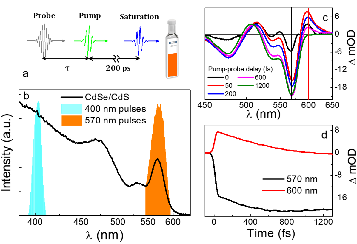
Figure 1: Design of the saturate-pump-probe experiment: (a) Timing sequence for the 3-pulses. Probe is always a chirped supercontinuum generated in BaF2. (b) Absorption spectrum of CdSe/CdS NCs dispersed in hexane, along with the spectra of the excitation pulses (400 and 570 nm). See text for details. c) Overlays of transient absorption spectra at the designated delays. d) Spectral cuts at the peaks of the 1S-1S bleach in black, and that of the low energy induced absorption in red.

II Results and Discussion

As shown in Fig. 1a, cold mono-exciton saturation is performed by an intense $400nm$ pulse followed by a delay of $200ps$ to allow completion of AR. Fig. 1b presents the absorption spectrum of the CdSe/CdS NCs along with the pulse spectra used for saturation and/or pump pulses in our experiments. Core/shells were chosen to eliminate the substantial effects of surface trapping characteristic of bare CdSe cores (Reiss et al., 2009; Rabouw et al., 2015). Fig. 1c presents an overlay of transient absorption spectra covering the first 2 ps of pump-probe delay. Similar to earlier studies by Kambhampati and coworkers (Kambhampati, 2011), buildup of the 1S-1S PIB is very rapid, increasing marginally during the subsequent cooling as depicted in the right panel. The photo-induced absorption band (PIA) to the red rises at least as rapidly and decays gradually for $\sim 2ps$. These trends are demonstrated by temporal cuts in panel d taken at wavelengths designated by the color-coded vertical lines in panel c of Fig. 1.

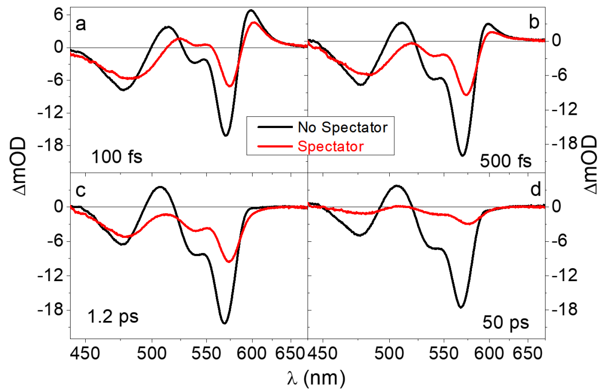
Figure 2: Comparison of 2- and 3-pulse TA measurements after weak $400nm$ pumping at a series of designated probe delays (a-d). Saturation pulses, like the pump, are derived from SHG of the laser fundamental.

Fig. 2 demonstrates how the presence of a spectator exciton changes the transient transmission spectra following a femtosecond $400nm$ excitation. We stress that in both experiments pump fluence has been controlled to ensure that the probability of absorbing more than one photon is negligible. Conversely, in the three-pulse experiment the saturation pulse is much more intense and ensures that $95\%$ of the crystallites absorb at least one photon. The four panels present transient spectra recorded in both experiments at selected delays between $100fs$ and $50ps$. Significant differences are apparent early on, a reduced bleach at the BE peak being the most obvious. The PIB band in three pulse experiments is also broader and blue shifted by $6nm$ ($\sim 20meV$). Another difference is that the PIA feature at $520nm$, apparent at all delays in 2-pulse data, is absent once spectator excitons are present. At 1.2 ps with carrier cooling over, the remaining PIB associated with state filling is precisely half as intense in the presence of spectators. These results are in qualitative agreement with our earlier study on PbSe, but spectator effects in CdSe are larger. At the $50ps$ delay the amplitude of the BE PIB with spectators has diminished by $\sim 70\%$ due to the presence of AR which does not affect two pulse pump-probe which involves long lived single excitons.

A glance at the first three delays in Fig. 2 shows that 2- and 3-pulse experiments differ consistently along the lines detailed above throughout carrier cooling. Notice that while spectral evolution from delay to delay is pronounced in both experiments, the difference between 2- and 3-pulse transient spectra at the same pump-probe delay remains nearly constant. This similarity is demonstrated in panel A of Fig. 3 as an overlay of the subtraction of the pairs presented in Fig. 2. Implications of this are first that carrier cooling dynamics is unaffected by presence of a BE spectator exciton in this range of delays. This is further demonstrated by band integrals producing difference dipole strength over the full spectral range probed in the experiment: $\Delta D\equiv\int_{c/670}^{c/450}\frac{\Delta OD}{\nu}d\nu$, and plotted in panel B of Fig. 3. Panels C and D display finite difference spectra extracted from 2- and 3-pulse data, defined as follows:

$$\Delta\Delta OD\left(\lambda,t,\Delta t\right) =\Delta OD\left(\lambda,t+\frac{\Delta t}{2}\right)$$

$$\,\,\,\,\,-\Delta OD\left(\lambda,t-\frac{\Delta t}{2}\right)$$

and serves to isolate spectral changes taking place over a specific interval of time. These spectra demonstrate essentially identical spectral evolution taking place in both experiments at delays of $>50fs$. They also show negligible alterations to the amplitude of PIB after this point, with spectral changes consisting primarily of the decay of a broad and structure-less absorption band covering most of the probed spectra range. A second implication is that dynamic processes leading to the conserved difference in spectra shown in Fig. 3A must be established considerably before the earliest 50 fs delay.

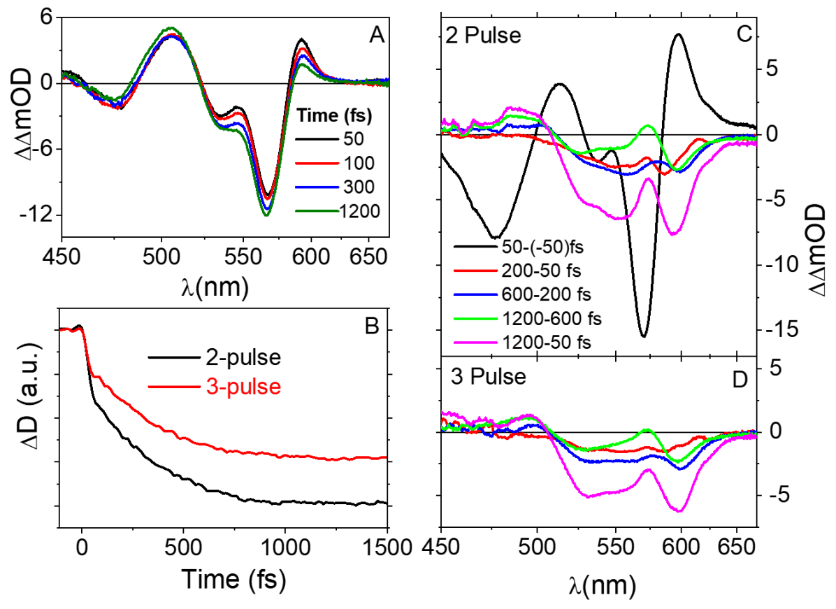
Figure 3: Comparison of spectral evolution in 2 and 3 pulse experiments pumping at $400nm$. A) Subtraction of the two data sets at a series of pump-probe delays from $0.05$ to $1.2ps$. B) Band integrals of the full probed range in the two experiments, demonstrating the identical cooling kinetics. C) Finite difference spectra obtained from the 2 pulse data isolating spectral changes taking place during sequential short intervals of carrier cooling. D) As in C for three pulse experiments. Notice that these spectra are essentially identical in both experiments for intervals starting after $50fs$.

These consequences will be the subject of a separate report dealing with carrier cooling dynamics. Here we concentrate on spectra established after cooling is complete. Clearly one of two assumptions discussed concerning the bleach amplitude introduced by the second exciton is wrong. Either the PIB is not linear in the number of excitons, or else not all excitons directly populate the lowest available conduction band states. In deciphering this riddle the factor of 2 in BE PIB between samples with or without resident excitons is a significant clue. Assume that the PIB is linear in $N$, what could block excitons from taking their place aside the existing spectator in the $1S^{e}$level? In order to fill that gap the pair of $1S^{e}$ electrons must be spin paired, and any disparity in correct orientation could delay the final step of relaxation. A random distribution of $\left|\uparrow\right\rangle$ and $\left|\downarrow\right\rangle$ spin orientations of relaxing electrons would prohibit half of the cooling electrons from the BE until one of the electron spins flip.

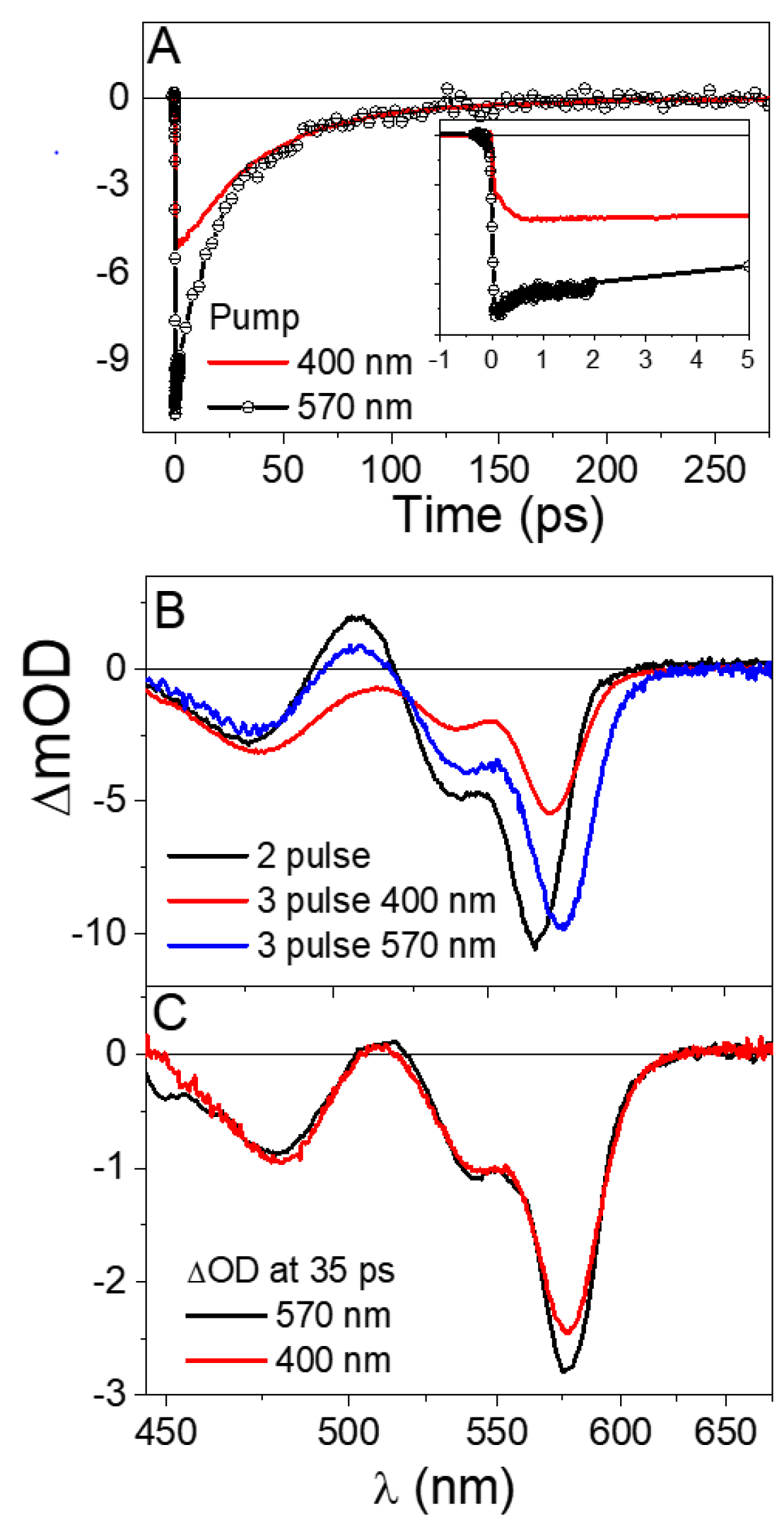
Figure 4: Spectral and temporal evolutions from 2-pulse and 3-pulse TA measurements upon pumping at the BE. (A) Comparison of band edge bleach kinetics for 3-pulse experiments for different pump excitation conditions: $570nm$ (solid line-circle, black) or $400nm$ (solid red line). Inset shows expanded scale up to 5 ps. (B) Comparison of TA spectra at $1.2ps$ for $570nm$ pump excitation in absence (black) and presence (red) of saturation pulses; (C) TA spectra of second exciton generated by pumping either at $570nm$ (black) or at 400 nm (red) at a pump-probe delay of $35ps$. Notice how the initially very different TA spectra of the two experiments are essentially identical as AR proceeds (See text).

Fortunately these assumptions can be tested experimentally. In our previous study of NC spectator effects pumping was conducted high in the inter-band continuum since there the cross section for absorption is unaffected by the existence of other excitons (Spoor et al., 2017; Cho et al., 2010). This provides a trivial method for ensuring an equal dose of additional excitons deposited in samples with or without spectators. However a second exciton can also be introduced to spectator containing samples by exciting directly at the BE. Quantitative comparison of the second exciton contribution to the PIB requires accounting for the changed absorption cross section of the pump due to the spectator excitons. The benefit is that pumping at the BE guarantees that all absorbed photons populate the $1S^{h}-1S^{e}$ state with or without preexisting spectator. The results of this experiment are shown in Fig. 4. Panel B presents TA spectra just after cooling for three different experiments, 2-pulse pump-probe, and two cases of saturate-pump-probe, the first pumping at $400nm$, and second exciting at 570 nm. Clearly, the bleach introduced by BE pumping in the presence of spectator excitons is on par with that apparent in 2-pulse pump-probe. The spectra are shifted due to the additional bi-exciton interaction involved, and the absence of residual absorption into the $1S^{h}-1S^{e}$ state when completely filled. Nonetheless, a band integral demonstrates that despite these anticipated discrepancies, the notion that BE PIB varies linearly with the population of the first cold excitons in the conduction band is upheld.

The alternative is that hot multi-excitons do not all relax to the lowest energy states. That due to spin orientation conflicts, relaxation to $1S^{e}$ is partially blocked. This leads to the following predictions: 1) An electron blocked from the BE by virtue of conflicting spin orientation will be stranded above in the $1P^{e}$ level and induce a partial PIB of the absorption into this band, and 2) AR kinetics in spin blockaded bi-excitons will appear to be slower at first since the decay of BE PIB will be partially canceled by gradual population of $1S^{e}$ following spin flips of the electron (assuming flips take place on a timescale of ~10 ps). Accordingly, the difference spectrum in three pulse experiments pumped at 400nm should approach that obtained by directly exciting into $570nm$ pumping once the frustrated bi-excitons have annealed to the BE. Our data confirm all these predictions. In panel B of Fig. 4, not only is the PIB by $400nm$ pumping $2$ times smaller than that induced at $570$, there is a missing PIA feature at $520nm$, consistent with partial state-filling of $1P^{e}$ due to stranded electrons. Panel A shows PIB decay kinetics for the same two experiments. As predicted, the AR dominated decay starts off much more rapidly for $570$ nm pumping. As the delay increases, both curves merge with a time constant of $\sim 15ps$. If spin frustrated bi-excitons undergo AR at the same rate as a relaxed one, this is consistent with a spin flip rate of $\sim 1/15ps^{-1}$ per electron (see discussion of spin-flip mechanism below). Finally, as shown in Fig. 4 panel C, the very different TA spectra at $1ps$, asymptotically converge once the remaining bi-excitons have relaxed to the BE, completing the consistency test with the spin conflict hypothesis.

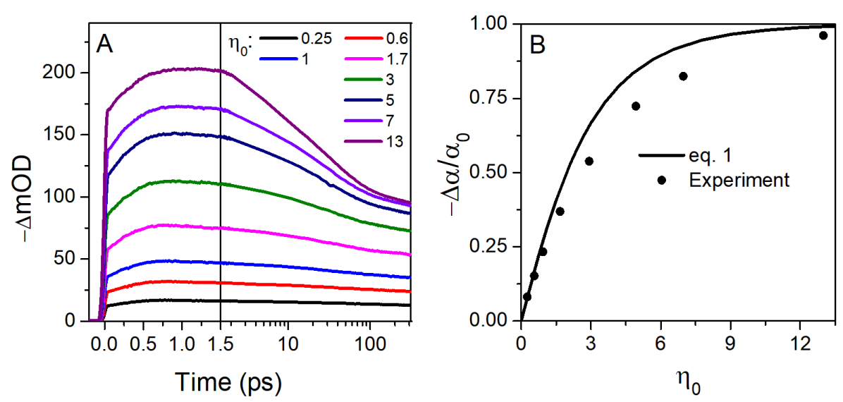
Figure 5: BE Bleach kinetics after $400nm$ excitation as a function of pump fluence. A) Kinetics from 0-125 ps, on a split time scale. First $1.5ps$ are plotted on a linear time axis, and thereafter data is plotted on a logarithmic scale. Pump fluences are presented in dimensionless units of 0, the average number of absorbed photons per nanocrystal at the front surface of the sample. B) Comparison of the measured 1S1S bleach saturation as a function of $\eta_{0}$ compared with a simulated one assuming fast decay of all excitons to the lowest available states, and state filling of ½ the BE band per exciton.

This selection rule for hot multi-exciton relaxation must hold in any matching scenario. As an example, panel A of Fig. 5 brings an overlay of pump-probe PIB kinetics for a broad range of $400nm$ excitation fluences. After determining the absorption cross section from the bleach amplitude at low pump fluence, as detailed in the supplementary information, each fluence is designated by $\eta_{0}\equiv\sigma_{A}\times\rho_{h\nu}$, the average number of absorbed photons per NC at the front surface of the sample. As $\eta_{0}$ increases, the PIB grows monotonically, increasing the portion of bleach which decays during AR. As expected, at the highest pump intensities, this decay accounts for nearly ½ of the bleach maximum at 1.5 ps. Knowing that absorption of the sample at $400nm$ is unchanged by absorbing even a number of photons, Poisson statistics integrated throughout the depth of the sample can be used to calculate the number density of NCs which have absorbed $N$ photons. Panel B brings the predicted fractional bleach amplitude assuming that all excitons relax directly to lowest available energy states, and that each 1S electron bleaches ½ of the 1S-1S exciton band (see details in supplementary information).

As $\eta_{0}$ increases, the actual bleach amplitude falls short of this prediction. We assign this to the same partially frustrated relaxation demonstrated in the spectator experiments. As photons are absorbed, excitons will rapidly relax to the lowest quantized states. After the first is in place, another will only be able to relax beside it if it has a correct spin orientation. This situation is worsened with increased pump fluence as the number of bi-excitons grows. Eventually as more and more excitons are generated, at least one of the additional electrons will have a matching spin state to fill the gap and complete BE bleaching. This explains the ultimate approach of the fractional to 1 when $\eta_{0}\gg 1$. Thus this limitation concerning cooling of multi-excitons is obvious even in very fundamental pump-probe experiments once analyzed quantitatively. It must accordingly be considered whenever the intense band edge exciton bleach is utilized to quantify exciton occupation numbers when multi-excitons are involved.

To test the plausibility of this interpretation, we developed a 3-state Lindblad master equation for describing the spin-flip dynamics.(Breuer and Petruccione, 2002) The lowest S^e state, well-separated by energy $\varepsilon_{S}$ from $P_{0}^{e}$, is populated by a spin-up spectator electron ($S_{\uparrow}^{e}$). Another hot electron subsequently promoted by the pump pulse is stranded in state $P_{-1\text{\textuparrow}}^{e}$, unable to populate $S_{\downarrow}^{e}$ due to Pauli blocking. Further relaxation can be achieved only by a spin-flip $P_{-1\text{\textuparrow}}^{e}\rightarrow P_{0\text{\textdownarrow}}^{e}$ facilitated by a spin-orbit interaction, after which the decay $P_{0\text{\textdownarrow}}^{e}\text{\textrightarrow}S_{\downarrow}^{e}$ takes place rapidly (Auger cooling). We neglect “Auger-spin-flip” cooling (where two nearly resonant excitons of opposite spin are Coulomb-coupled: $\left(nP_{\uparrow}^{h}-P_{\uparrow}^{e}\right)\text{\textrightarrow}\left(mP_{\text{\textuparrow}}^{h}-P_{\text{\textuparrow}}^{e}\right)$ for reasons detailed in the supplementary information). Spin reorientation due to interaction with nuclear spins is also not included in our model. Phonon modes serve as a (classical) heat bath for taking up any energy mismatch. Setting the energy origin at P_e^0, the total Hamiltonian of the system and bath is

$$H =2\Delta\left|P_{-1\uparrow}^{e}\right\rangle\left\langle P_{-1\uparrow}^{e}\right|-\varepsilon_{S}\left|S_{\downarrow}^{e}\right\rangle\left\langle S_{\downarrow}^{e}\right|$$

$$+s\left(\left|P_{0\downarrow}^{e}\right\rangle\left\langle P_{-1\uparrow}^{e}\right|+\left|P_{-1\uparrow}^{e}\right\rangle\left\langle P_{0\downarrow}^{e}\right|\right)$$

$$+\sum_{j}\left(A_{01}^{j}\left|P_{0\downarrow}^{e}\right\rangle\left\langle S_{\uparrow}^{e}\right|+cc\right)\frac{p_{j}}{m_{j}}$$

$$+\sum_{j}\left(\frac{p_{j}^{2}}{2m_{j}}+\frac{1}{2}m_{j}\omega_{j}^{2}x_{j}^{2}\right)$$

Where $-\varepsilon_{S}$ ($2\Delta$) are the energy difference between the $S^{e}$ ($P_{-1}^{e}$) and the $P_{0}^{e}$ levels respectively, $s$ is the spin-flip matrix element. For weak electron-nuclear interactions we neglect all but the linear coupling to the nuclear velocity $p_{j}/m_{j}$.

As a concrete system we considered a $\text{Cd}_{36}\text{Se}_{36}$ cluster with structure taken from Ref. Gutsev et al., 2014 and relaxed using the Q-CHEM density functional (DFT) code (Shao et al., 2015) at the PBE/6-31G level. This gave the following parameter values: $\varepsilon_{S}=890cm^{-1}$ and $2\Delta=2000cm^{-1}$, while the spin orbit coupling $s$ was dependent sharply on the identity of the hole states correlated with the electrons and varied in the range $0-200cm^{-1}$. Lindblad master equations were set up in accordance with the Hamiltonian for $T=300K$. $A_{01}$ was determined by requiring that the $P_{0\downarrow}^{e}\rightarrow S_{\downarrow}^{e}$ decay time be $0.5ps$ (Guyot-Sionnest et al., 1999; Klimov et al., 1999; Klimov, 2000; Sewall et al., 2006; Kambhampati, 2011; Cooney et al., 2007). With these parameter values we obtained the temporal populations of the adiabatic states shown in Figure 6(b). State 2 is of $P_{-1\uparrow}^{e}$ character and at $t=0$ has close to $0.85$ population which decays through spin-flips, at a rate of about $10ps$, to State 1, which is of $P_{0\text{\textdownarrow}}^{e}$ character. This latter state stays slightly populated at later times as it continuously feeds the S state which is of $S_{\text{\textdownarrow}}^{e}$ character. The rate of S state population through spin flipping is much longer than the Auger cooling alone, and takes place on a $10ps$ time-scale. The sensitivity of these conclusions to the parameters of the model is rather small, and the fastest rate that can be reached is $\sim 4ps$. These calculations show that a realistic model of the material under study predicts rates for spin flip limited cooling in the presence of a band edge spectator which are consistent with that measured experimentally. This is bolstered by a demonstration of the moderate dependence of this rate on the material parameters.

Figure 6: (a) A schematic depiction of the lowest states at the conduction band-edge, used for modeling the decay rate of an excited-blocked electron. See text for explanation. (b) Temporal Lindblad master equation populations for the three adiabatic states of the model, showing the fast and slow decay transients. (c) Sensitivity of the long life time $\tau$ to the spin-orbit and level displacement parameters ($s$ and $\Delta$ respectively) of the model.

Relaxation of optically-polarized spin states in nanocrystals has been investigated extensively, in part to test if semiconductor quantum dots can provide a platform for spintronics applications (Hanson and Awschalom, 2008). In the case of colloidal nanocrystals, studies have concentrated on electronic states limited to the lowest $1S_{3/2}1S^{e}$ exciton manifold (Gupta et al., 1999; Scholes, 2004; Kim et al., 2009). With spin relaxation components spanning ps to hundreds of nanosecond timescales, results of those experiments are not directly comparable to our findings for a number of reasons. First, the fine structure levels of the exciton ground state are only defined in terms of correlated hole and electron microstates, while the observable described here should involve the electron alone (Klimov et al., 1999; Sewall et al., 2006). Furthermore, analysis of polarization dependent pump-probe experiments conducted in a grating geometry clarifies that none of the separable phases of spin polarization decay are dominated by electron spin flips alone (Wong et al., 2009). Finally, while spin orbit coupling defining the ground exciton sub levels stems from the “p” orbital basis of the valence band, in our case its origin is in non-zero orbital angular momentum related with the envelope $1P^{e}$ function. Our measurements thus cover a very different process. All that can be said in comparison is that the observed timescale of a few tens of ps lies within the broad range characterizing the multi-exponential decay of optically induced spin polarization in the $1S_{3/2}1S^{e}$ exciton manifold. Only future investigations of how the electron spin flip rate measured here is effected by temperature, particle size and crystal morphology will teach more about its relation to other magnetic relaxation processes in nanocrystals.

Supplementary Information

III Theoretical model

We assume The electron states exhibit a separate ground state, $S^{e}$, $800cm^{-1}$ below a group of three excited electron states, $P_{0,\pm 1}^{e}$. The splitting between the p-states is on the order of $2\Delta=100cm^{-1}$. We have also performed a TDDFT calculation and estimated various spin-orbit couplings, between excited states. Because of the multitude of hole states there is no one number, but a spectrum of couplings, spanning a range of $s=10-300cm^{-1}$.

In Fig. 7 we describe our model for the experiment in CdSe NCs. There are two excitons, one is “cold”, in the band edge, due to the first experimental pulse with an up-spin electron in the $S^{e}$ state and the second has its hole at the top of the valence manifold but its up-spin electron is in one of the P states of the and it is blocked from further decay onto the $S^{e}$ level because of Pauli exclusion.

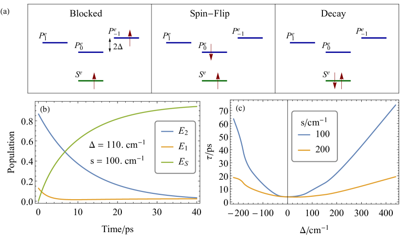
Figure 7: (a) Left panel: the up-spin electron in the $P_{-1\uparrow}^{e}$ level (say) is blocked from decay into the edge level $S_{\downarrow}^{e}$ due to Pauli exclusion. Middle panel: A spin-orbit induced spin-flip occurs: $P_{-1\uparrow}^{e}\to P_{0\downarrow}^{e}$. Right panel: The down-spin electron decay $P_{0\downarrow}^{e}\to S_{\downarrow}^{e}$. (b) The populations of the three adiabatic states as a function of time for the indicated values of $\Delta$ and $s$. (c) a sensitivity analysis checking time scale for the final cooling to the parameters.

III.1 Dissipative dynamics under spin-flip

We first neglect spin-orbit coupling. In this case, we consider the electronic Hamiltonian of the levels $P_{-1\uparrow}^{e}$, $P_{0\downarrow}^{e}$ and $S_{\downarrow}^{e}$:

$$H_{S} =\left(\begin{array}[]{ccc}2\Delta&0&0\\ 0&0&0\\ 0&0&-\varepsilon_{S}\end{array}\right).$$ (4)

where we assumed that the energy of the $P_{0\downarrow}^{e}$ level is zero and that of the $P_{-1\uparrow}^{e}$ level is displaced by $2\Delta$ while that of the $S^{e}$ is below by $\varepsilon_{S}>0$.

The total Hamiltonian $H_{tot}$ describing the coupling of to a bath of phonons is

$$H_{tot} =H_{B}+H_{S}+\sum_{j}\left(\frac{p_{j}}{m_{j}}\right)\left(\begin{array}[]{ccc}0&0&0\\ 0&0&A_{j}^{12}\\ 0&A_{j}^{21}&0\end{array}\right)$$ (8)

where $A_{j}^{12}=A_{j}^{21*}$ are the non-adiabatic coupling terms and

$$H_{B}=\sum_{j}\left(\frac{p_{j}^{2}}{2m_{j}}+\frac{1}{2}m_{j}\omega_{j}^{2}x_{j}^{2}\right)$$ (9)

is the phonon Hamiltonian. Notice that there is no non-adiabatic coupling of the $P_{-1\uparrow}^{e}$ level and the $S_{\downarrow}^{e}$ level because of the different spins.

Now, introduce the spin coupling $s$ between levels $P_{-1\uparrow}^{e}$ and $P_{0\downarrow}^{e}$. The 3-level Hamiltonian in Eq. 4 is thus generalized to

$$H_{S} =\left(\begin{array}[]{ccc}2\Delta&s&0\\ s&0&0\\ 0&0&-\varepsilon_{S}\end{array}\right).$$ (13)

We diagonalize $H_{a}=U^{\dagger}H_{S}U$, using

$$U =\left(\begin{array}[]{ccc}\cos\theta/2&-\sin\theta/2&0\\ \sin\theta/2&\cos\theta/2&0\\ 0&0&1\end{array}\right)$$ (17)

giving:

$$H_{a} \equiv\left(\begin{array}[]{ccc}E_{1}&0&0\\ 0&E_{2}&0\\ 0&0&E_{S}\end{array}\right)$$ (21)

$$=2R\left(\begin{array}[]{ccc}\cos^{2}\theta/2&0&0\\ 0&-\sin^{2}\theta/2&0\\ 0&0&-\varepsilon_{S}/2R\end{array}\right)$$ (25)

where, $R$ and $\theta$ are defined by requiring $\Delta=R\cos\theta$ and $s=R\sin\theta$. The total Hamiltonian then becomes:

$$H_{tot}^{a}=H_{a}+H_{B}+\sum_{j}\left(\frac{p_{j}}{m_{j}}\right)\left(\begin{array}[]{ccc}0&0&\tilde{A}_{j}^{01}\\ 0&0&\tilde{A}_{j}^{12}\\ \tilde{A}_{j}^{10}&\tilde{A}_{j}^{21}&0\end{array}\right).$$ (26)

where $\tilde{A}_{j}^{12}=\tilde{A}_{j}^{21*}=A_{j}^{12}\cos\theta/2$ and $\tilde{A}_{j}^{02}=\tilde{A}_{j}^{20*}=A_{j}^{12}\sin\theta/2$ now couple both adiabatic P-states with the S-state because the spin-orbit coupling mixes the up- and down-spin states.

In order to study the dynamics, we assume the reduced $3\times 3$ density matrix $\sigma_{ij}$ obeys the Lindblad equation(Breuer and Petruccione, 2002):

$$\dot{\sigma}\left(t\right)=-\frac{i}{\hbar}\left[H_{a}+H_{1a},\sigma\right]+\text{$\mathfrak{D}$}\sigma\left(t\right)$$ (27)

where the dissipative and hermitian bath effects are given as:

$$\text{$\mathfrak{D}$}\sigma =\sum_{\omega}\gamma\left(\omega\right)\left[L\left(\omega\right)\sigma L\left(\omega\right)^{\dagger}-\frac{1}{2}\left\{L\left(\omega\right)^{\dagger}L\left(\omega\right),\sigma\right\}\right]$$ (28)

$$H_{1} =\sum_{\omega}S\left(\omega\right)L\left(\omega\right)^{\dagger}L\left(\omega\right)$$ (29)

where the summation is over discrete frequencies, $\omega_{m}=m\frac{2\pi}{T_{d}}$ where $T_{d}$ is the discretization period and

$$\Gamma\left(\omega\right)=\frac{1}{2}\gamma\left(\omega\right)+iS\left(\omega\right)=\int_{0}^{T_{d}}e^{i\omega t}\left\langle\frac{p\left(t\right)}{m}\frac{p\left(0\right)}{m}\right\rangle_{\beta}dt$$ (30)

is the bath frequency velocity autocorrelation function at inverse temperature $\beta$ (see Appendix A). For the two resonant frequencies, $\hbar\omega_{20}=\varepsilon_{S}+2R\cos^{2}\theta/2$ and $\hbar\omega_{21}=\varepsilon_{S}-2R\sin^{2}\theta/2$ and present in our Hamiltonian, we have the following Lindblad operator

$$L_{\omega} =\hbar^{-1}\left(\begin{array}[]{ccc}0&0&\tilde{A}^{02}\delta_{\omega,\omega_{20}}\\ 0&0&\tilde{A}_{j}^{12}\delta_{\omega,\omega_{21}}\\ \tilde{A}_{j}^{20}\delta_{-\omega,\omega_{20}}&\tilde{A}_{j}^{21}\delta_{-\omega,\omega_{21}}&0\end{array}\right)$$ (34)

which is a Liouvillian eigenstate $\left[H,L_{\omega}\right]=\hbar\omega L_{\omega}$. With this, the dissipation above term in (28) becomes

$$\text{$\mathfrak{D}$}\sigma =\left(\begin{array}[]{ccc}-D_{20}\sigma_{00}+D_{02}\sigma_{22}&-\frac{D_{20}+D_{21}}{2}\sigma_{01}&-\frac{D_{20}+D_{02}+D_{12}}{2}\sigma_{02}\\ -\frac{D_{20}+D_{21}}{2}\sigma_{10}&-D_{21}\sigma_{11}+D_{12}\sigma_{22}&-\frac{D_{02}+D_{12}+D_{21}}{2}\sigma_{12}\\ -\frac{D_{20}+D_{02}+D_{12}}{2}\sigma_{20}&-\frac{D_{02}+D_{12}+D_{21}}{2}\sigma_{21}&-\left(D_{02}+D_{12}\right)\sigma_{22}+D_{20}\sigma_{00}+D_{21}\sigma_{11}\end{array}\right),$$ (38)

where (see Appendix_A, Eq. (73)):

$$D_{02} =a\omega_{02}\left(\left\langle n\right\rangle_{\beta\hbar\omega_{02}}+1\right)\sin^{2}\theta/2,$$ (39)

$$D_{20} =a\omega_{02}\left\langle n\right\rangle_{\beta\hbar\omega_{02}}\sin^{2}\theta/2,$$ (40)

$$D_{12} =a\omega_{12}\left(\left\langle n\right\rangle_{\beta\hbar\omega_{12}}+1\right)\cos^{2}\theta/2,$$ (41)

$$D_{21} =a\omega_{12}\left\langle n\right\rangle_{\beta\hbar\omega_{12}}\cos^{2}\theta/2.$$ (42)

with $a=T_{d}\frac{\left|A_{12}\right|^{2}}{2m\hbar}$ the dimensionless non-adiabatic parameter.

III.2 Why spin-flip Auger coupling is weak

In CdSe NCs Auger coupling is a major nonradiative energy dissipation mechanism in excited NCs (Klimov et al., 2000). The direct coupling between excitons involves the matrix elements :

$$\left\langle 0\left|c_{j\uparrow}^{\dagger}c_{b\uparrow}\hat{V}c_{a\uparrow}^{\dagger}c_{i\uparrow}\right|0\right\rangle =\delta_{ij}\delta_{ab}2\left(2V_{vssv}-V_{svsv}\right)n_{s}n_{v}$$

$$+2\delta_{ij}\left(2V_{btta}-V_{btat}\right)n_{t}$$

$$-2\delta_{ab}\left(2V_{ittj}-V_{itjt}\right)n_{t}$$ (43)

$$+2\left(V_{ibja}-V_{ibaj}\right)$$

where $\hat{V}=\sum_{stuv}\sum_{\sigma\sigma^{\prime}=\uparrow\downarrow}V_{utsv}c_{u\sigma}^{\dagger}c_{t\sigma^{\prime}}^{\dagger}c_{s\sigma^{\prime}}c_{v\sigma}$ is the Coulomb interaction in second quantization, $\psi_{s}\left(\boldsymbol{r}\right)$, $\psi_{t}\left(\boldsymbol{r}\right)$, $\psi_{u}\left(\boldsymbol{r}\right)$, $\psi_{v}\left(\boldsymbol{r}\right)$ are one-electron (Hartree-Fock) eigenstates and

$$V_{utsv} =\frac{1}{2}\iint\frac{\left[\psi_{u}\left(\boldsymbol{r}^{\prime}\right)\psi_{v}\left(\boldsymbol{r}^{\prime}\right)\right]\left[\psi_{t}\left(\boldsymbol{r}\right)\psi_{s}\left(\boldsymbol{r}\right)\right]}{\left|\boldsymbol{r}-\boldsymbol{r}^{\prime}\right|}d\boldsymbol{r}d\boldsymbol{r}^{\prime}$$ (44)

and for which the creation and annihilation commutation relations are:

$$\left[c_{u\sigma}^{\dagger},c_{s\sigma^{\prime}}\right]_{+}=\delta_{\sigma\sigma^{\prime}}\delta_{uv}$$ (45)

The first term in Eq. (43), $i=j$ and $a=b$ is a “diagonal element” and is not interesting for our purpose. When either $a=b$ or $i=j$ (but not both) it’s the second (or third) term that is important. This is either that the electron changes state while the hole is a spectator or vice versa. Suppose it’s the electron changing from $a$ to $b$ while the hole stays put in $i=j$, the coupling then involves the Coulomb interaction of a electron charge distribution $2\psi_{b}\left(\boldsymbol{r}\right)\psi_{a}\left(\boldsymbol{r}\right)$ with the entire electron density 2$\sum_{i=1}^{N_{e}/2}\left|\psi_{i}\left(\boldsymbol{r}\right)\right|^{2}$ in the nanocrystals (corrected by a much smaller exchange term, since only $\psi_{t}$’s that overlap with both $\psi_{a}$ and $\psi_{b}$ contribute). So, as long as $\psi_{a}\left(\boldsymbol{r}\right)$ and $\psi_{b}\left(\boldsymbol{r}\right)$ strongly overlap in space this is very strong.

However, if the coupling involves spin-flip, the corresponding Auger element evaluates just one term

$$\left\langle 0\left|c_{j\downarrow}^{\dagger}c_{b\downarrow}\hat{V}c_{a\uparrow}^{\dagger}c_{i\uparrow}\right|0\right\rangle=2V_{biaj}$$ (46)

which is the Coulomb interaction between two charge of distributions one is $\psi_{b}\left(\boldsymbol{r}\right)\psi_{j}\left(\boldsymbol{r}\right)$ and the other $\psi_{i}\left(\boldsymbol{r}\right)\psi_{j}\left(\boldsymbol{r}\right)$, for this to be strong one requirement is good electron-hole overlap for each of the two excitons and that they are reasonably close so that the Coulomb interaction is considerable. The direct Auger involves interacting of the dynamical electron with all other electrons in the system while the spin-flip process is just a local two-electron interaction.

Summarizing, Auger processes which are typically efficient mechanisms for biexciton decay in nanocrystals are much slower when a spin-flip is involved.

III.3 Results of model

The model involves 5 parameters: the temperature $T$, taken to be 300K, energy offset of the $S_{\downarrow}^{e}$ state $\varepsilon_{S}$ with respect to the $P_{e}^{0}$ state, the dimensionless non-adiabatic coupling strength $a$, the P-level splitting $\Delta$ and the spin-flip coupling strength $s$.

Using Q-CHEM (Shao et al., 2015)) we have performed ab initio calculations on relaxed $\text{Cd}_{36}\text{Se}_{36}$ (see Ref. Gutsev et al., 2014). We used the PW91 functional and a small basis set (see a separate supplementary information file). The calculations reveal the typical CdSe NC frontier orbital structure: a dense manifold of hole states and a sparse one for electron states above it, with an optical gap, of 1.1eV. We also determined from the calculation $\varepsilon_{S}=0.1eV$ and $\Delta=500\mu E_{h}$. Finally we determined the parameter $a=0.14$, by requiring that the rate of decay $P\to S$ without a spectator (without the requirement for spin-flip) be $0.5ps$, in accordance with the known experiment estimates.

The spin-flip mechanism considered here is caused by the spin-orbit coupling between a pair of singlet and triplet excitons. The singlet exciton, originally formed by the laser pulse, has decayed in a fast time scale to the blocked state, where the electron is in a $P^{e}$ excited state with the spin. The triplet exciton is similar except that the excited $P^{e}$ electron has flipped its spin (and changed to a different $P^{e}$ state, see Fig. 7a). Due to the large density of hole states in our model $\text{Cd}_{36}\text{Se}_{36}$ system, we were forced to produce a large number of exciton states: the electron in the first 35 excitons was in the lowest $S^{e}$ state and only the hole was in an excited state and only in exciton number 36, at energy of 1.34eV, was the first to have an electron in an excited $P^{e}$ state . Out of the first 200 excitons we selected the few that were 1) dominated by a single electron-hole excitation, and 2) the electron was in one of the two lowest diabatic $P^{e}$ states. Due to non-adiabatic effects these states mix slightly and we label the adiabatic states as $1$ (mostly $P_{0}^{e}$) and $2$ (mostly $P_{-1}^{e}$). We focused attention on a small energy band 1.34-1.56eV which contained about 100 excitons (out of the 200 calculated). Of those, only nine were singlet excitons, four with the electron in state 1 and five with the electron in state $2$. We also identified sixteen such triplet excitons, nine having an electron in state $1$ and seven an electron in state $2$. Within these excitons there are four types of SO couplings: $\left\langle S_{1}\left|H_{SO}\right|T_{1}\right\rangle$, $\left\langle S_{2}\left|H_{SO}\right|T_{2}\right\rangle$, $\left\langle S_{1}\left|H_{SO}\right|S_{2}\right\rangle$ and $\left\langle S_{2}\left|H_{SO}\right|S_{1}\right\rangle$. The first pair of matrix elements describe a hole spin-flip (the electron stays put) while the second pair describe an electron spin-flip. The calculations show, that the hole spin-flip (which is not of interest for our mechanism) involved a strong coupling averaging at $200cm^{-1}$ and peaking at $480cm^{-1}$. On the other hand, electron spin-flip SO couplings typically have 5 times weaker couplings: averaging at $50cm^{-1}$ and peaking at $144cm^{-1}$. These calculated ab initio values prompted us to take a representative value of $s=100cm^{-1}$ and then also comparing to $s=200cm^{-1}$as a stability analysis.

With these parameters we solved the Lindblad equation and taking (see Fig. 7(a)) and obtained the adiabatic state populations $\sigma_{ii}\left(t\right)$, $i=2,1,S^{e}$. The system starts in (diabatic) state $P_{-1}^{e}$ which populates mainly state 2 and due to spin-orbit coupling also a bit of state 2 (this small part fasyer to the $S^{e}$ state). Then the main part of the population decays at a time scale of 10ps, reaching equilibrium.

We also checked the sensitivity of the results to $s$ and $\Delta$ and obtained the lifetime in Fig.7(c). It is interesting to see that for large spin-orbit couplings even 200$cm^{-1}$ the spin-flip effect slow down to about 5 ps.

IV Materials and Methods

IV.1 Synthesis of CdSe QDs core

A mixture of cadmium oxide (CdO) and oleic acid (OA) in a molar ratio of 1:4 and 7.5 mL of 1-octadecene (ODE) was put in a 25 mL three-neck flask. The reaction mixture was degassed for 1 h at $100^{o}C$ under vacuum. Under nitrogen, the temperature was then raised to $300^{o}C$ until the solution turned clear, indicating the formation of cadmium oleate. Then the solution was cooled, and the octadecylamine (ODA) was added in a molar ratio of 1:8 (Cd/ODA). Afterward, the solution was heated to $280^{o}C$ , and 8 mL of 0.25 M trioctylphosphine selenide (TOPSe) was injected under vigorous stirring. The growth was terminated after 16 minute by rapid injection of 10 ml of ODE and the reaction mixture was further cooled down by water bath. As prepared core CdSe QDs were precipitated twice with a 2-propanol/ethanol mixture (1:1−1:2), separated by centrifugation, and redissolved in hexane.

IV.2 Synthesis of CdSe QDs coated with 1 monolayer (ML) of CdS

The 0.1 M Cd precursor was prepared by dissolving 0.1 mmol of cadmium acetate ($Cd(Ac)_{2}$) and 0.2 mmol of hexadecylamine (HAD) in 10 mL of ODE at $100^{o}C$ inside a nitrogen-filled glovebox. The 0.1 M S precursor was prepared by dissolving 0.1 mmol of sulfur in 10 mL of ODE at $100^{o}C$ . The coating procedure has been adapted from previous report (Grumbach et al., 2015). Initially, 14.8 mL of ODE was degassed under vacuum for 1 h at $100^{o}C$. The ODE was cooled to $65^{o}C$, and a solution of 7.4 × 10−4 mmol CdSe QDs in hexane was injected. Then, the Cd precursor solution was added at $65^{o}C$. After degassing for 10 min under vacuum at $65^{o}C$ , the S precursor was added. The reaction mixture was quickly heated to $100^{o}C$ and allowed to remain for 2 h at this temperature. Then the nanoparticles were precipitated with a mixture of 2-propanol and ethanol (1:1−1:2), separated by centrifugation, and re-dissolved in hexane.

IV.3 Pump-probe measurements

The CdSe/CdS core/shell QDs were prepared under inert atmosphere, inside a nitrogen filled glove box. The sample was placed in air-tight 0.25 mm quartz cell for the pump-probe measurements. A home built multi-pass amplified Ti-Sapphire laser producing 30 fs pulses at 790 nm with 1 mJ of energy at 1 kHz repetition rate was used to generate the fundamental. The laser fundamental was split into different paths for generation of probe and pump pulses. The pump pulses at 400 nm were produced by frequency doubling of the fundamental 800 nm pulses, whereas the pump pulses at 570 nm were generated by second harmonic generation of signal (at 1140 nm) from an optical parametric amplifier (TOPAS 800, Light Conversion). The pump pulses at 570 nm were compressed using grating-mirror compressor set up. The spectra of two pump pulses are shown in Figure 1b. The supercontinuum probe pulses were generated by focusing 1200 nm output pulses of another optical parametric amplifier (TOPAS Prime, Light Conversion) on a 2 mm BaF2 crystal. The pump and probe beams were directed to the sample using all reflective optics. The spot size of the pump on the sample was at least two times larger compared to that of the probe beam.

Conventional two-pulse pump-probe experiments were carried out with white light ranging from 420-700 nm as probe and 400 nm or 570 nm pulses as pump, with low fluence such that the average no. of exciton per nanocrystals, η $\approx$ 0.2. In the case of three-pulse measurements, the same two-pulse pump-probe experiments were repeated in presence of another saturation pulse at 400 nm which arrives ~200 ps earlier than the pump pulses. Raw data from three-pulse measurements show a constant bleach (~10% that of initial single exciton bleach) signal even long time after completion of Auger recombination, suggesting that ~10% of the total no. of NCs were not saturated by the strong saturation pulses. Thus, raw data from three-pulse measurements was first subtracted by 10% of two-pulse data and then the subtracted dataset was divided by 0.9 so that the final three-pulse data represents for fully saturated sample.

V Experimental determination of absorption cross section of the CdSe/CdS core/shell nanocrystals

The absorption cross section of the CdSe/CdS core/shell QDs was experimentally determined according to previously reported procedure (Gdor et al., 2015). Fig. 8A demonstrates the 1S1S transition bleach as a function of pump-probe delay after $400nm$ excitation, for a series of different excitation photon fluxes as indicated in the inset. All these experiments were carried out with weak excitation fluences such that the bleach changes linearly. Fig. 8B shows a plot of $\mathit{\Delta}$I/I0 vs. photon flux change. From the linear fit of these experimental data points and known the 2-fold degeneracy of 1S1S transition of the CdSe dots, the slope of the fit gives the absorption cross section value at the pump wavelength, $\sigma_{400}=(2.7\pm 0.1)\times 10^{-15}cm^{2}$.

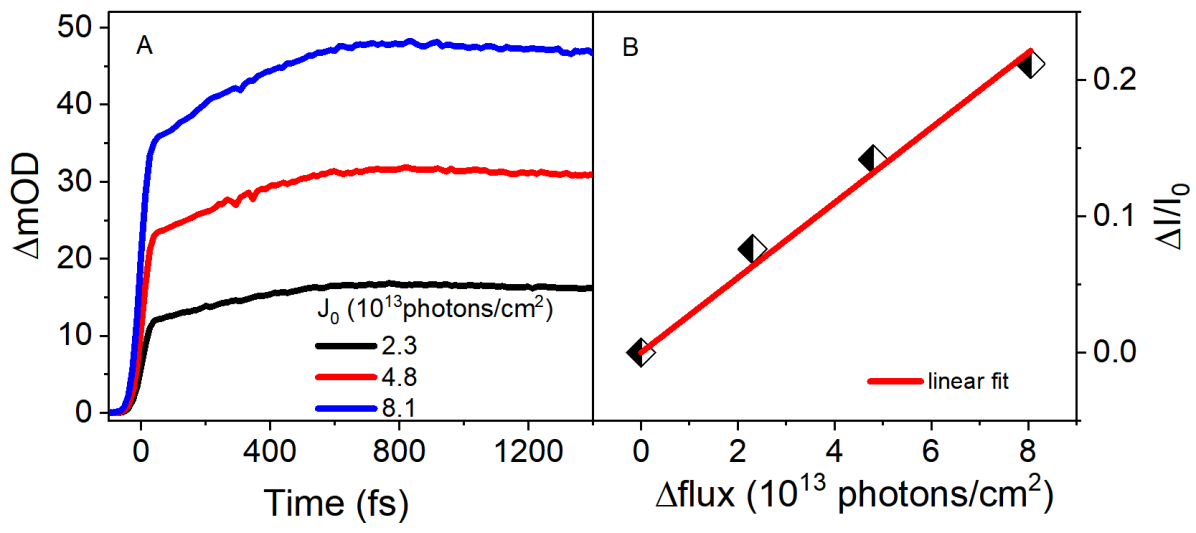
Figure 8: Determination of absorption cross section of CdSe/CdS core/shell nanocrystals. (A) Plot of 1S1S bleach signal (at 570 nm) vs. pump-probe delay (up to 1.4 ps) after excitation with 400 nm pulses, at different excitation pump fluences as presented in the inset; (B) Plot of fractional absorption change vs. photon flux and linear fit of the experimental data. The absorption cross section can be calculated from the slope of this fit.

VI Simulation of excitation pump fluence dependence on band edge bleach

Defining $J_{0}$ and $J_{\infty}$ as the pump photon flux (photons/$cm^{2}$) in the front and back surfaces of an optically thick sample cell, and $\sigma$ as the absorption cross-section ($cm^{2}$) at the pump wavelength, the average no. of absorbed photons per nanocrystal at the front ($\eta_{0}$) and back surface ($\eta_{\infty}$) are:

$$J_{0}\sigma=\eta_{0},\,\,\,\,\,J_{\infty}\sigma=\eta_{\infty}.$$ (47)

Denoting $\rho_{T}$ as the total density/$cm^{2}$ of NC in the sample, assuming pump wavelength absorption is unaffected by existing excitons the ratio $\eta_{\infty}/\eta_{0}$ must equal to $e^{-\rho_{T}\sigma}$ and therefore:

$$\rho_{T} =\frac{1}{\sigma}\log\left(\frac{\eta_{0}}{\eta_{\infty}}\right)$$ (48)

$$=\frac{1}{\sigma}\int_{\eta_{\infty}}^{\eta_{0}}\frac{d\eta}{\eta}.$$

For an optically thin slab of nanodots at a given $\eta$ the probability for a quantum dot to absorb $N$ pump photons follows the Poisson distribution,

$$P_{N}\left(\eta\right)=\frac{e^{-\eta}\eta^{N}}{N!},$$ (49)

with $\sum_{N=0}^{\infty}P_{N}=1$ and $P_{0}=e^{-\eta}$. Accordingly, the probability of absorbing at least one photon is $P_{N>0}\left(\eta\right)=1-e^{-\eta}$ and the probability of absorbing more than one photon per nanocrystals is given by, $P_{N>1}\left(\eta\right)=1-e^{-\eta}-\eta e^{-\eta}$.

Returning to an optically thick sample where pump intensity reduces significantly over the cell, all the above can be used to calculate the density per unit area of particles which have absorbed $N$ pump photons as:

$$\rho_{N}=\frac{1}{\sigma}\int_{\eta_{0}}^{\eta_{\infty}}P_{N}\left(\eta\right)\frac{d\eta}{\eta}.$$ (50)

Finally before deriving expressions for the fractional BE bleach we require two more densities, $\rho_{N>0}$ the density per unit area of dots absorbing at one or more photons, and $\rho_{N>1}$ the density of those absorbing two or more photons:

$$\rho_{N>0} =\frac{1}{\sigma}\int_{\eta_{0}}^{\eta_{\infty}}\left(1-e^{\eta}\right)\frac{d\eta}{\eta},$$ (51)

$$\rho_{N>1} =\frac{1}{\sigma}\int_{\eta_{0}}^{\eta_{\infty}}\left(1-e^{\eta}-\eta e^{\eta}\right)\frac{d\eta}{\eta}.$$ (52)

To derive an expression for the intensity dependent fractional bleaching at the band edge (BE) we use the equations for $\rho_{T}$, $\rho_{N>0}$ and $\rho_{N>1}$ along with $\eta_{\infty}$,$\eta_{0}$,and $\sigma_{BE}$ the cross section at the first exciton peak. Notice that when pumping high in the inter-band continuum, $\sigma$ is often more than 10 times larger than $\sigma_{BE}$. Assuming linear bleaching of the BE transition up to a degeneracy of 2, $\alpha_{BE}$ the sample band edge absorbance after excitation (and carrier cooling) $\alpha_{BE,\eta_{0}}$ is obtained by integrating over the pump fluences throughout the cell:

$$\alpha_{BE,\eta_{0}}=\left(\rho_{T}-\frac{\rho_{N>0}}{2}-\frac{\rho_{N>1}}{2}\right)\sigma_{BE}.$$ (53)

The fraction of residual absorption after pump excitation is accordingly,

$$\frac{\alpha_{BE,\eta_{0}}}{\alpha_{BE}} =\frac{2\rho_{T}-\rho_{N>0}-\rho_{N>1}}{2\rho_{T}}.$$ (54)

Substituting Eqs. (48), (50)-(52) into Eq. (54) we obtain:

$$\frac{\alpha_{BE,\eta_{0}}}{\alpha_{BE}}=\frac{1}{\log\left|\eta_{0}/\eta_{\infty}\right|}\int_{\eta_{\infty}}^{\eta_{0}}\left(e^{-\eta}+0.5\eta e^{-\eta}\right)\frac{d\eta}{\eta},$$ (55)

from which the final fractional bleach is

$$\frac{\Delta\alpha_{BE,\eta_{0}}}{\alpha_{BE}}=1-\frac{1}{\log\left|\eta_{0}/\eta_{\infty}\right|}\int_{\eta_{\infty}}^{\eta_{0}}\left(e^{-\eta}+0.5\eta e^{-\eta}\right)\frac{d\eta}{\eta},$$ (56)

and this is the expression used to simulate the plot of $\Delta\alpha/\alpha_{0}$vs $\eta_{0}$in Fig. 5B of the manuscript.

Appendix A Harmonic correlation function

The time correlation function of the Harmonic Oscillator at temperature $\beta$ is

$$C\left(t,\beta\right) =\frac{1}{m^{2}}\sum_{n}\frac{e^{-\beta E_{n}}}{Z}\left\langle n\left|\hat{p}\left(t\right)\hat{p}\left(0\right)\right|n\right\rangle$$ (57)

$$=\frac{1}{m^{2}}\sum_{nm}\frac{e^{-\beta E_{n}}}{Z}e^{iE_{nm}t}\left\langle n\left|\hat{p}\left|m\right\rangle\left\langle m\right|\hat{p}\right|n\right\rangle$$ (58)

$$=\frac{1}{m^{2}}\sum_{nm}\frac{e^{-\beta E_{n}}}{Z}e^{iE_{nm}t}\left|\left\langle n\left|\hat{p}\right|m\right\rangle\right|^{2}$$ (59)

where $M\hbar=P^{2}t$

$$Z\left(\beta\right)=\sum_{n=0}^{\infty}e^{-\beta\hbar\omega n}=\frac{1}{1-e^{-\beta\hbar\omega}}$$ (60)

$$\left\langle n\left|\hat{p}\right|m\right\rangle =i\sqrt{\frac{\hbar m\omega}{2}}\left\langle n\left|\hat{a}^{\dagger}-\hat{a}\right|m\right\rangle$$ (61)

$$=i\sqrt{\frac{\hbar m\omega}{2}}\left(\sqrt{m+1}\delta_{n,m+1}-\sqrt{m}\delta_{n,m-1}\right)$$ (62)

hence

$$\left|\left\langle n\left|\hat{p}\right|m\right\rangle\right|^{2}=\frac{m\hbar\omega}{2}\left(\left(m+1\right)\delta_{n,m+1}+m\delta_{n,m-1}\right)$$ (63)

$$C\left(t,\beta\right) =\frac{\hbar\omega}{2m}\left(e^{i\omega t}+e^{-i\omega t}e^{\beta\hbar\omega}\right)\frac{1}{Z}\sum_{n=0}^{\infty}ne^{-\beta n\hbar\omega}$$ (64)

$$=\frac{\hbar\omega}{2m}\left(e^{i\omega t}+e^{-i\omega t}e^{\beta\hbar\omega}\right)\left\langle n\right\rangle_{\beta}$$ (65)

and

$$\left\langle n\right\rangle_{\beta,\omega} =\frac{1}{Z}\sum_{n=0}^{\infty}ne^{-\beta n\hbar\omega}$$ (66)

$$=-\frac{1}{\hbar\omega}\frac{\partial}{\partial\beta}\ln Z$$ (67)

$$=\frac{1}{\hbar\omega}\frac{\partial}{\partial\beta}\ln\left(1-e^{-\beta\hbar\omega}\right)$$ (68)

$$=\frac{1}{e^{\beta\hbar\omega}-1}$$ (69)

Clearly

$$\left\langle n\right\rangle_{\beta,\omega}+1 =e^{\beta\hbar\omega}\left\langle n\right\rangle_{\beta,\omega}$$ (70)

finally,

$$C\left(t,\beta\right) =\frac{\hbar\omega}{2m}\left\langle n\right\rangle_{\beta\omega}\left(e^{i\omega t}+e^{-i\omega t}e^{\beta\hbar\omega}\right)$$ (71)

$$=\frac{\hbar\omega}{2m}\left(\left\langle n\right\rangle_{\beta\omega}e^{i\hbar\omega t}+e^{-i\hbar\omega t}\left(\left\langle n\right\rangle_{\beta\omega}+1\right)\right)$$ (72)

if we assume that the frequency is discrete $\omega_{m}=\frac{2\pi}{T_{d}}m$ where $m$ is integer then the response function of Eq. (30) assumes the following form:

$$\gamma\left(\pm\omega,\beta\right) =T_{d}\frac{\hbar\omega}{2m}\left(\left\langle n\right\rangle_{\beta\omega}+\frac{1\pm 1}{2}\right).$$ (73)

Appendix B Cd36H36 Input file

This is the Q-CHEM input file, including the nuclear configuration and the basis set.

⬇

$molecule

0 1

Cd 2.26266696 0.80336407 -6.46510988

Cd 2.26266696 0.80336407 6.46510988

Cd -0.43389281 -2.49625428 -6.40155700

Cd -0.43389281 -2.49625428 6.40155700

Cd -1.88543621 1.45902174 -6.49895678

Cd -1.88543621 1.45902174 6.49895678

Cd -4.10780789 -1.20308722 -4.75283647

Cd -4.10780789 -1.20308722 4.75283647

Cd 0.83699863 4.07573258 -4.85280032

Cd 0.83699863 4.07573258 4.85280032

Cd 3.09910097 -2.83326887 -4.78577050

Cd 3.09910097 -2.83326887 4.78577050

Cd 2.83458308 0.82682770 -2.31844206

Cd 2.83458308 0.82682770 2.31844206

Cd -0.68852828 -3.06559991 -2.27167782

Cd -0.68852828 -3.06559991 2.27167782

Cd -2.12214994 1.94667024 -2.34781506

Cd -2.12214994 1.94667024 2.34781506

Cd -4.03854179 -1.39280936 0.00000000

Cd 3.40396851 -2.47907728 0.00000000

Cd 0.34766961 4.16957255 0.00000000

Cd 5.42916889 3.32370962 0.00000000

Cd -5.60011141 3.27040539 0.00000000

Cd 0.37762859 -6.53714690 0.00000000

Cd 4.57345019 3.90346038 -4.31177363

Cd 4.57345019 3.90346038 4.31177363

Cd -5.68257664 2.23505087 -4.30733764

Cd -5.68257664 2.23505087 4.30733764

Cd 1.23344351 -6.03770026 -4.29679356

Cd 1.23344351 -6.03770026 4.29679356

Cd 3.23078991 6.19612775 -2.10464336

Cd 3.23078991 6.19612775 2.10464336

Cd -7.18687857 0.06708793 -2.12106907

Cd -7.18687857 0.06708793 2.12106907

Cd 3.90521114 -5.97673874 -2.11084867

Cd 3.90521114 -5.97673874 2.11084867

Se -1.50427559 -4.48878986 0.00000000

Se 4.45358377 0.70162186 0.00000000

Se -2.80571365 3.38671429 0.00000000

Se 1.48190896 6.73882226 0.00000000

Se -6.81740331 -1.70124355 0.00000000

Se 5.16109123 -4.67106092 0.00000000

Se -2.63307265 -0.89017218 -2.35055978

Se -2.63307265 -0.89017218 2.35055978

Se 0.64055415 2.65897350 -2.37385332

Se 0.64055415 2.65897350 2.37385332

Se 1.95497191 -1.90482171 -2.34921571

Se 1.95497191 -1.90482171 2.34921571

Se 1.68463259 -7.73753003 -2.14176246

Se 1.68463259 -7.73753003 2.14176246

Se 5.83081241 5.07118510 -2.12602700

Se 5.83081241 5.07118510 2.12602700

Se -7.32389824 2.89605112 -2.15331364

Se -7.32389824 2.89605112 2.15331364

Se -1.08500310 -4.57016641 -4.66077668

Se -1.08500310 -4.57016641 4.66077668

Se 4.38648158 1.17716053 -4.69347086

Se 4.38648158 1.17716053 4.69347086

Se -3.14171439 3.20684327 -4.70192993

Se -3.14171439 3.20684327 4.70192993

Se 2.74601892 6.05192643 -4.87800129

Se 2.74601892 6.05192643 4.87800129

Se -6.73130484 -0.37782115 -4.85442287

Se -6.73130484 -0.37782115 4.85442287

Se 3.98914709 -5.42724163 -4.87277230

Se 3.98914709 -5.42724163 4.87277230

Se -2.72602690 -1.09340696 -7.16667357

Se -2.72602690 -1.09340696 7.16667357

Se 0.45328051 2.74250861 -7.26553396

Se 0.45328051 2.74250861 7.26553396

Se 2.14166044 -1.86454113 -7.21620233

Se 2.14166044 -1.86454113 7.21620233

$end

$rem

JOBTYPE sp

SCF_FINAL_PRINT 1

SCF_CONVERGENCE 6

PRINT_ORBITALS 1000

MOLDEN_FORMAT TRUE

basis gen

exchange PW91

SCF_ALGORITHM diis_gdm

CIS_N_ROOTS 100

CIS_SINGLETS true

CIS_TRIPLETS true

CIS_CONVERGENCE 6

CALC_SOC true

SYMMETRY false

UNRESTRICTED false

SYM_IGNORE true

max_scf_cycles 500

mem_total 200000

mem_static 2000

$end

$basis

Se 0

S 3 1.00

2480.6268140 0.1543289673

451.8492708 0.5353281423

122.2880464 0.4446345422

SP 3 1.00

206.1578780 -0.0999672292 0.1559162750

47.90665727 0.3995128261 0.6076837186

15.58073180 0.7001154689 0.3919573931

SP 3 1.00

17.63999414 -0.2277635023 0.0049515112

5.380760465 0.2175436044 0.5777664691

2.076064666 0.9166769611 0.4846460366

SP 3 1.00

1.2146442970 -0.3088441215 -0.1215468600

0.4482801363 0.0196064117 0.5715227604

0.1979652346 1.1310344420 0.5498949471

D 3 1.00

17.63999414 0.2197679508

5.380760465 0.6555473627

2.076064666 0.2865732590

****

Cd 0

S 3 1.00

4950.2619050 0.1543289673

901.6963856 0.5353281423

244.0342313 0.4446345422

SP 3 1.00

433.4469385 -0.0999672292 0.1559162750

100.7237469 0.3995128261 0.6076837186

32.75848861 0.7001154689 0.3919573931

SP 3 1.00

52.59279235 -0.2277635023 0.0049515111

16.04247800 0.2175436044 0.5777664691

6.189686744 0.9166769611 0.4846460366

SP 3 1.00

5.674851796 -0.3306100626 -0.1283927634

2.209757875 0.0576109533 0.5852047641

0.9727408566 1.1557874500 0.5439442040

SP 3 1.00

0.5949150981 -0.3842642607 -0.3481691526

0.3203250000 -0.1972567438 0.6290323690

0.1414931855 1.3754955120 0.6662832743

D 3 1.00

52.59279235 0.2197679508

16.04247800 0.6555473627

6.189686744 0.2865732590

D 3 1.00

3.642963976 0.1250662138

1.418551290 0.6686785577

0.6244497700 0.3052468245

****

$end

References

- König et al. (2010) Dirk König, K Casalenuovo, Y Takeda, G Conibeer, JF Guillemoles, R Patterson, LM Huang, and MA Green, “Hot carrier solar cells: Principles, materials and design,” Physica E 42, 2862–2866 (2010).
- Pandey and Guyot-Sionnest (2009) Anshu Pandey and Philippe Guyot-Sionnest, “Hot electron extraction from colloidal quantum dots,” J. Phys. Chem. Lett. 1, 45–47 (2009).
- Saeed et al. (2014) S Saeed, EMLD De Jong, K Dohnalova, and T Gregorkiewicz, “Efficient optical extraction of hot-carrier energy,” Nat. Commun. 5, 4665 (2014).
- Konstantatos and Sargent (2013) G. Konstantatos and E. H. Sargent, Colloidal Quantum Dot Optoelectronics and Photovoltaics (Cambridge University Academic Press, 2013).
- Williams et al. (2013) Kenrick J. Williams, Cory A. Nelson, Xin Yan, Liang-Shi Li, and Xiaoyang Zhu, “Hot electron injection from graphene quantum dots to tio2,” ACS Nano 7, 1388–1394 (2013), pMID: 23347000, https://doi.org/10.1021/nn305080c .
- Li et al. (2017) Mingjie Li, Saikat Bhaumik, Teck Wee Goh, Muduli Subas Kumar, Natalia Yantara, Michael Grätzel, Subodh Mhaisalkar, Nripan Mathews, and Tze Chien Sum, “Slow cooling and highly efficient extraction of hot carriers in colloidal perovskite nanocrystals,” Nat. Commun. 8, 14350 (2017).
- Woggon et al. (1996) U Woggon, H Giessen, F Gindele, O Wind, B Fluegel, and N Peyghambarian, “Ultrafast energy relaxation in quantum dots,” Phys. Rev. B 54, 17681 (1996).
- Nozik (2001) Arthur J Nozik, “Spectroscopy and hot electron relaxation dynamics in semiconductor quantum wells and quantum dots,” Annu. Rev. Phys. Chem. 52, 193–231 (2001).
- Guyot-Sionnest et al. (1999) P. Guyot-Sionnest, M. Shim, C. Matranga, and M. Hines, “Intraband relaxation in cdse quantum dots,” Phys. Rev. B 60, R2181–R2184 (1999).
- Klimov et al. (1999) VI Klimov, DW McBranch, CA Leatherdale, and MG Bawendi, “Electron and hole relaxation pathways in semiconductor quantum dots,” Phys. Rev. B 60, 13740 (1999).
- Klimov (2000) V. I. Klimov, “Optical nonlinearities and ultrafast carrier dynamics in semiconductor nanocrystals,” J. Phys. Chem. B 104, 6112–6123 (2000).
- Sewall et al. (2006) Samuel L Sewall, Ryan R Cooney, Kevin EH Anderson, Eva A Dias, and Patanjali Kambhampati, “State-to-state exciton dynamics in semiconductor quantum dots,” Phys. Rev. B 74, 235328 (2006).
- Kambhampati (2011) Patanjali Kambhampati, “Hot exciton relaxation dynamics in semiconductor quantum dots: radiationless transitions on the nanoscale,” J. Phys. Chem. C 115, 22089–22109 (2011).
- Cooney et al. (2007) Ryan R Cooney, Samuel L Sewall, Eva A Dias, DM Sagar, Kevin EH Anderson, and Patanjali Kambhampati, “Unified picture of electron and hole relaxation pathways in semiconductor quantum dots,” Phys. Rev. B 75, 245311 (2007).
- Gdor et al. (2012) I. Gdor, H. Sachs, A. Roitblat, D. B. Strasfeld, M. G. Bawendi, and S. Ruhman, “Exploring exciton relaxation and multiexciton generation in Pbse nanocrystals using hyperspectral near-IR probing,” ACS Nano 6, 3269–3277 (2012).
- Gdor et al. (2013) Itay Gdor, Chunfan Yang, Diana Yanover, Hanan Sachs, Efrat Lifshitz, and Sanford Ruhman, “Novel spectral decay dynamics of hot excitons in pbse nanocrystals: A tunable femtosecond pump–hyperspectral probe study,” J. Phys. Chem. C 117, 26342–26350 (2013).
- Spoor et al. (2015) Frank CM Spoor, Lucas T Kunneman, Wiel H Evers, Nicolas Renaud, Ferdinand C Grozema, Arjan J Houtepen, and Laurens DA Siebbeles, “Hole cooling is much faster than electron cooling in pbse quantum dots,” ACS Nano 10, 695–703 (2015).
- Spoor et al. (2017) Frank CM Spoor, Stanko Tomić, Arjan J Houtepen, and Laurens DA Siebbeles, “Broadband cooling spectra of hot electrons and holes in pbse quantum dots,” ACS Nano 11, 6286–6294 (2017).
- Efros and Efros (1982) A. L. Efros and A. L. Efros, “Interband absorption of light in a semiconductor sphere,” Soviet Physics Semiconductors-Ussr 16, 772–775 (1982).
- Esch et al. (1990) V Esch, B Fluegel, G Khitrova, HM Gibbs, Xu Jiajin, K Kang, SW Koch, LC Liu, SH Risbud, and N Peyghambarian, “State filling, coulomb, and trapping effects in the optical nonlinearity of cdte quantum dots in glass,” Phys. Rev. B 42, 7450 (1990).
- Klimov (2007) Victor I Klimov, “Spectral and dynamical properties of multiexcitons in semiconductor nanocrystals,” Annu. Rev. Phys. Chem. 58, 635–673 (2007).
- Kambhampati (2012) Patanjali Kambhampati, “Multiexcitons in semiconductor nanocrystals: a platform for optoelectronics at high carrier concentration,” J. Phys. Chem. Lett. 3, 1182–1190 (2012).
- Klimov et al. (2000) Victor I Klimov, Alexander A Mikhailovsky, DW McBranch, Catherine A Leatherdale, and Moungi G Bawendi, “Quantization of multiparticle auger rates in semiconductor quantum dots,” Science 287, 1011–1013 (2000).
- Gdor et al. (2015) Itay Gdor, Arthur Shapiro, Chunfan Yang, Diana Yanover, Efrat Lifshitz, and Sanford Ruhman, “Three-pulse femtosecond spectroscopy of pbse nanocrystals: 1s bleach nonlinearity and sub-band-edge excited-state absorption assignment,” ACS Nano 9, 2138–2147 (2015).
- Leatherdale et al. (2002) C. A. Leatherdale, W. K. Woo, F. V. Mikulec, and M. G. Bawendi, “On the absorption cross section of cdse nanocrystal quantum dots,” J. Phys. Chem. B 106, 7619–7622 (2002).
- Osborne et al. (2004) SW Osborne, P Blood, PM Smowton, YC Xin, A Stintz, D Huffaker, and LF Lester, “Optical absorption cross section of quantum dots,” J. Phys.: Condens. Matter 16, S3749 (2004).
- Jasieniak et al. (2009) Jacek Jasieniak, Lisa Smith, Joel Van Embden, Paul Mulvaney, and Marco Califano, “Re-examination of the size-dependent absorption properties of cdse quantum dots,” J. Phys. Chem. C 113, 19468–19474 (2009).
- Efros and Rosen (2000) A. L. Efros and M. Rosen, “The electronic structure of semiconductor nanocrystals,” Annu. Rev. Mater. Sci. 30, 475–521 (2000).
- Hendry et al. (2006) E. Hendry, M. Koeberg, F. Wang, H. Zhang, C. de Mello Donega, D. Vanmaekelbergh, and M. Bonn, “Direct observation of electron-to-hole energy transfer in cdse quantum dots,” Phys. Rev. Lett. 96, 057408–4 (2006).
- Reiss et al. (2009) Peter Reiss, Myriam Protiére, and Liang Li, “Coreshell semiconductor nanocrystals,” Small 5, 154–168 (2009).
- Rabouw et al. (2015) Freddy T. Rabouw, Roman Vaxenburg, Artem A. Bakulin, Relinde J. A. van Dijk-Moes, Huib J. Bakker, Anna Rodina, Efrat Lifshitz, Alexander L. Efros, A. Femius Koenderink, and Daniël Vanmaekelbergh, “Dynamics of intraband and interband auger processes in colloidal core-shell quantum dots,” ACS Nano 9, 10366–10376 (2015).
- Cho et al. (2010) Byungmoon Cho, William K. Peters, Robert J. Hill, Trevor L. Courtney, and David M. Jonas, “Bulklike hot carrier dynamics in lead sulfide quantum dots,” Nano Letters 10, 2498–2505 (2010), pMID: 20550102, https://doi.org/10.1021/nl1010349 .
- Breuer and Petruccione (2002) Heinz-Peter Breuer and F. Petruccione, The theory of open quantum systems (Oxford University Press, Oxford ; New York, 2002) pp. xxi, 625 p.
- Gutsev et al. (2014) LG Gutsev, NS Dalal, and GL Gutsev, “Structure and magnetic properties of (cdse) 9 doped with mn atoms,” Computational Materials Science 83, 261–268 (2014).
- Shao et al. (2015) Yihan Shao, Zhengting Gan, Evgeny Epifanovsky, Andrew T.B. Gilbert, Michael Wormit, Joerg Kussmann, Adrian W. Lange, Andrew Behn, Jia Deng, Xintian Feng, Debashree Ghosh, Matthew Goldey, Paul R. Horn, Leif D. Jacobson, Ilya Kaliman, Rustam Z. Khaliullin, Tomasz Kus, Arie Landau, Jie Liu, Emil I. Proynov, Young Min Rhee, Ryan M. Richard, Mary A. Rohrdanz, Ryan P. Steele, Eric J. Sundstrom, H. Lee Woodcock III, Paul M. Zimmerman, Dmitry Zuev, Ben Albrecht, Ethan Alguire, Brian Austin, Gregory J. O. Beran, Yves A. Bernard, Eric Berquist, Kai Brandhorst, Ksenia B. Bravaya, Shawn T. Brown, David Casanova, Chun-Min Chang, Yunqing Chen, Siu Hung Chien, Kristina D. Closser, Deborah L. Crittenden, Michael Diedenhofen, Robert A. DiStasio Jr., Hainam Do, Anthony D. Dutoi, Richard G. Edgar, Shervin Fatehi, Laszlo Fusti-Molnar, An Ghysels, Anna Golubeva-Zadorozhnaya, Joseph Gomes, Magnus W.D. Hanson-Heine, Philipp H.P. Harbach, Andreas W. Hauser, Edward G. Hohenstein, Zachary C. Holden, Thomas-C. Jagau, Hyunjun Ji, Benjamin Kaduk, Kirill Khistyaev, Jaehoon Kim, Jihan Kim, Rollin A. King, Phil Klunzinger, Dmytro Kosenkov, Tim Kowalczyk, Caroline M. Krauter, Ka Un Lao, Adele D. Laurent, Keith V. Lawler, Sergey V. Levchenko, Ching Yeh Lin, Fenglai Liu, Ester Livshits, Rohini C. Lochan, Arne Luenser, Prashant Manohar, Samuel F. Manzer, Shan-Ping Mao, Narbe Mardirossian, Aleksandr V. Marenich, Simon A. Maurer, Nicholas J. Mayhall, Eric Neuscamman, C. Melania Oana, Roberto Olivares-Amaya, Darragh P. O’Neill, John A. Parkhill, Trilisa M. Perrine, Roberto Peverati, Alexander Prociuk, Dirk R. Rehn, Edina Rosta, Nicholas J. Russ, Shaama M. Sharada, Sandeep Sharma, David W. Small, Alexander Sodt, Tamar Stein, David Stock, Yu-Chuan Su, Alex J.W. Thom, Takashi Tsuchimochi, Vitalii Vanovschi, Leslie Vogt, Oleg Vydrov, Tao Wang, Mark A. Watson, Jan Wenzel, Alec White, Christopher F. Williams, Jun Yang, Sina Yeganeh, Shane R. Yost, Zhi-Qiang You, Igor Ying Zhang, Xing Zhang, Yan Zhao, Bernard R. Brooks, Garnet K.L. Chan, Daniel M. Chipman, Christopher J. Cramer, William A. Goddard III, Mark S. Gordon, Warren J. Hehre, Andreas Klamt, Henry F. Schaefer III, Michael W. Schmidt, C. David Sherrill, Donald G. Truhlar, Arieh Warshel, Xin Xu, Alan Aspuru-Guzik, Roi Baer, Alexis T. Bell, Nicholas A. Besley, Jeng-Da Chai, Andreas Dreuw, Barry D. Dunietz, Thomas R. Furlani, Steven R. Gwaltney, Chao-Ping Hsu, Yousung Jung, Jing Kong, Daniel S. Lambrecht, WanZhen Liang, Christian Ochsenfeld, Vitaly A. Rassolov, Lyudmila V. Slipchenko, Joseph E. Subotnik, Troy Van Voorhis, John M. Herbert, Anna I. Krylov, Peter M.W. Gill, and Martin Head-Gordon, “Advances in molecular quantum chemistry contained in the q-chem 4 program package,” Mol. Phys. 113, 184–215 (2015).
- Hanson and Awschalom (2008) Ronald Hanson and David D. Awschalom, “Coherent manipulation of single spins in semiconductors,” Nature 453, 1043 (2008).
- Gupta et al. (1999) J. A. Gupta, D. D. Awschalom, X. Peng, and A. P. Alivisatos, “Spin coherence in semiconductor quantum dots,” Phys. Rev. B 59, R10421–R10424 (1999).
- Scholes (2004) Gregory D. Scholes, “Selection rules for probing biexcitons and electron spin transitions in isotropic quantum dot ensembles,” J. Chem. Phys. 121, 10104–10110 (2004).
- Kim et al. (2009) Jeongho Kim, Cathy Y. Wong, and Gregory D. Scholes, “Exciton fine structure and spin relaxation in semiconductor colloidal quantum dots,” Acc. Chem. Res. 42, 1037–1046 (2009).
- Wong et al. (2009) B. M. Wong, M. Piacenza, and F. Della Sala, “Absorption and fluorescence properties of oligothiophene biomarkers from long-range-corrected time-dependent density functional theory,” Phys. Chem. Chem. Phys. 11, 4498–4508 (2009).
- Grumbach et al. (2015) Nathan Grumbach, Richard K. Capek, Evgeny Tilchin, Anna Rubin-Brusilovski, Junfeng Yang, Yair Ein-Eli, and Efrat Lifshitz, “Comprehensive route to the formation of alloy interface in core/shell colloidal quantum dots,” The Journal of Physical Chemistry C 119, 12749–12756 (2015), https://doi.org/10.1021/acs.jpcc.5b03086 .