EC-GSM-IoT Network Synchronization with Support for Large Frequency Offsets

Abstract

(EDGE)-based Extended-Coverage for the (EC-GSM-IoT) is a promising candidate for the billion-device cellular (cIoT), providing similar coverage and battery life as Narrow-Band IoT (NB-IoT). The goal of $20\text{\,}\mathrm{dB}$ coverage extension compared to EDGE poses significant challenges for the initial network synchronization, which has to be performed well below the thermal noise floor, down to SNR Signal to Noise Ratio (SNR) of $-8.5\text{\,}\mathrm{dB}$. We present a low-complexity synchronization algorithm supporting up to $50\text{\,}\mathrm{kHz}$ initial frequency offset, thus enabling the use of a low-cost $\pm 25\text{\,}\mathrm{ppm}$ oscillator. The proposed algorithm does not only fulfill the 3rd Generation Partnership Project (3GPP) requirements, but surpasses them by $3\text{\,}\mathrm{dB}$, enabling communication with SNR SNR of $-11.5\text{\,}\mathrm{dB}$ or a maximum coupling loss of up to $170.5\text{\,}\mathrm{dB}$.

I Introduction

Cellular networks have enabled five billion people to connect to the Internet. This number is expected to rise further, with 4th Generation (4G) and 5th Generation (5G) standards meeting the high throughput and low latency requirements of mobile phones. In addition to this, it is estimated that billions of devices will also be directly connected to the Internet. The 3GPP has developed three new standards to address the needs of this Internet of Things (IoT): EC-GSM-IoT, Long Term Evolution (LTE) Cat-NB (NB-IoT), and LTE Cat-M (eMTC) all provide better coverage and reduce both cost and power consumption for low-rate devices [1].

The vast majority of cIoT devices currently use (GPRS)/EDGE to connect to the Internet [2]. For these, EC-GSM-IoT provides an easy path to improved energy efficiency and a $20\text{\,}\mathrm{dB}$ coverage improvement. EC-GSM-IoT specifies $164\text{\,}\mathrm{dB}$ of Maximum Coupling Loss (MCL) and an expected battery life of more than 10 years, matching the other cIoT standards. Additionally, EDGE support provides instantaneous global coverage and allows the throughput to scale up to $355\text{\,}\mathrm{kbit}\text{p}\mathrm{s}$, comparable to half-duplex LTE Cat-M1. Further, EC-GSM-IoT is expected to have the lowest module cost of the 3GPP standards [2].

The problem of synchronizing to a legacy GSM carrier has been extensively studied and several low-complexity solutions exist [3, 4]. For EC-GSM-IoT, however, the sensitivity requirement is $20\text{\,}\mathrm{dB}$ more stringent, and the signal level is now well below the thermal noise floor. The legacy algorithms are unable to cope with this, and new approaches are required to synchronize at SNRs as low as $-8.5\text{\,}\mathrm{dB}$.

In this paper, we present an algorithm, which is able to perform the EC-GSM-IoT network synchronization down to SNR SNR of $-11.5\text{\,}\mathrm{dB}$ in a low-band STatic (ST) channel. The support for frequency offsets of up to $50\text{\,}\mathrm{kHz}$ allows the use of a $\pm 25\text{\,}\mathrm{ppm}$ crystal oscillator and, therefore, enables a low overall module cost. Compared to [5], the MF boundary can be detected at $-14.4\text{\,}\mathrm{dB}$ instead of $-11\text{\,}\mathrm{dB}$ SNR in ST ST channel, and the average synchronization time at $-8.5\text{\,}\mathrm{dB}$ SNR has been reduced by $56\text{\,}\mathrm{\char 37\relax}$ to $1.3\text{\,}\mathrm{s}$. The proposed Frequency Offset Estimation (FOE) can accurately estimate the frequency offset at $-8.5\text{\,}\mathrm{dB}$ SNR.

The remainder of this paper is structured as follows: Section II introduces the EC-GSM-IoT MF, the proposed synchronization procedure, the system model, and the synchronization requirements. The proposed algorithms are discussed in detail in Section III. Finally, the performance for synchronizing to a known carrier and the cell search are evaluated in Sections IV and V.

II EC-GSM-IoT Network Synchronization

II-A Multi-Frame Structure

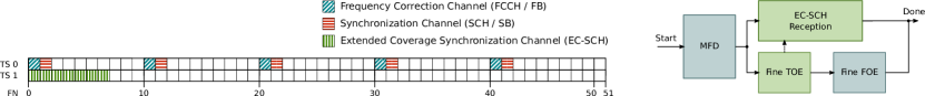
Figure 1: Left: EC-GSM-IoT MF. In addition to the legacy FBs and SCHs, seven blind repetitions of the EC-SCH are present on TS 1 of the frames $06$. TimeSlots $27$ are not shown, since they are not used for the synchronization. Right: Synchronization flow for the proposed algorithm.

Fig. 1 shows the elements in the EC-GSM-IoT MF, which enable the network synchronization. This $235\text{\,}\mathrm{ms}$ long structure is repeated on the BCCH carrier. It consists of $51$ frames with eight TSs each. Five FBs are transmitted on TS 0 of frames 0, 10, 20, 30, and 40. The legacy SCH follows exactly one frame later and carries the current frame number and the Base Station (BS) identity code. Devices may not be able to decode the SCH below the noise floor, and can use the Extended-Coverage (EC-SCH) with 28 blind repetitions over four MFs instead. The presence of the EC-SCH indicates that the networks supports EC-GSM-IoT.

II-B Synchronization Procedure

The proposed algorithm performs the synchronization in four sequential steps as shown in Fig. 1. First, the boundary Detection (MFD) finds a coarse estimate for the start time of the MF and the frequency offset, using the FBs. After the frequency offset has been corrected for, the fine time offset is estimated using the EC-SCH training sequences. At the same time, the decoding of the EC-SCH is started. The fine FOE can be started, as soon as the fine time offset is known. The device is ready to receive the Extended Coverage (EC-BCCH), once the EC-SCH has been successfully decoded, and may transmit, once the fine FOE is completed.

II-C System Model

We use the same noise figure as the 3GPP reference document: $\text{NF}=$5\text{\,}\mathrm{dB}$$ [6]. The noise bandwidth is $\text{BW}=$200\text{\,}\mathrm{kHz}$$ and the sampling frequency is $f_{s}=$270.8\text{\,}\mathrm{kHz}$$. The receiver is powered on at a random time, and the initial frequency offset is uniformly distributed between $\pm f_{o,\max}=\pm Rf_{c}$. $R$ is the error relative to the carrier frequency $f_{c}$. The simulations for the low bands were performed at $f_{c}=$900\text{\,}\mathrm{MHz}$$ and at $f_{c}=$2\text{\,}\mathrm{GHz}$$ for the high bands.

Since the oscillator is a significant factor in the system cost, it is desirable to use a low-cost crystal oscillator for cIoT cIoT application. These typically have an initial accuracy of $R=$25\text{\,}\mathrm{ppm}$$. In the high bands, this corresponds to a maximum frequency offset of $\pm 50\text{\,}\mathrm{kHz}$. This offset can be corrected by tuning the oscillator, or compensated for in the digital baseband.

II-D Synchronization Requirements

A device is synchronized to the network, if it has successfully decoded the EC-SCH, achieved timing synchronization, and corrected for the offset of the local oscillator. The requirements from the EC-GSM-IoT standard are as follows [1]:

R1

The device must be able to synchronize to the BCCH carrier within 2 seconds after power-on, which corresponds to successfully decoding the EC-SCH.

R2a

Before the first transmission, the timing offset with respect to the BS must be below $\pm 1$ symbol periods.

R2b

Before the first transmission, the relative frequency offset with respect to the BS must be below $\pm 0.1\text{\,}\mathrm{ppm}$.

Requirement R1 has to be met at the Input Signal Level (ISL) for reference performance of the EC-BCCH, while Requirements R2a and R2b have to be met at the ISL for reference performance of the EC-SCH. These requirements differ for the low and high frequency bands, and are specified for three radio channels conditions: ST, Typical Urban (TU)1.2, and TU50. The latter are fading with a mobile speed of $1.2\text{\,}\mathrm{km}\text{/}\mathrm{h}$ and $50\text{\,}\mathrm{km}\text{/}\mathrm{h}$. The EC-SCH and EC-BCCH ISL for the ST channels correspond to SNR SNR of $-8.5\text{\,}\mathrm{dB}$ and $-7.5\text{\,}\mathrm{dB}$. The SNRs for the low band TU1.2 channels are $-5.5\text{\,}\mathrm{dB}$ and $-3.5\text{\,}\mathrm{dB}$ respectively. Since no maximum miss rate is specified for Requirement R1, we will use the same as specified for the EC-SCH BLock Error Rate (BLER): $10\text{\,}\mathrm{\char 37\relax}$ misses.

The $2\text{\,}\mathrm{s}$ from Requirement R1 equal approximately eight MFs. In the worst-case, it takes seven MFs to receive a complete set of 28 blind EC-SCH repetitions. Therefore, the MFD should usually only require a single MF. If the MFD takes more than four MFs, it is no longer possible to collect all 28 blind repetitions of the EC-SCH within $2\text{\,}\mathrm{s}$.

III Network Synchronization Algorithm

III-A Fine Frequency Offset Estimation

The fine FOE is performed as the last step of the synchronization. This allows us to discuss it as a stand-alone problem, assuming perfect timing synchronization. The FOE estimates the offset of the local oscillator compared to the BS using the regularly transmitted FBs. Each FB consists of a pure sine at $f_{s}/4=$67.7\text{\,}\mathrm{kHz}$$ for $148$ symbol durations. The problem of estimating the frequency of a sine in Additive White Gaussian Noise (AWGN) is a well-studied problem, and the Cramér-Rao Lower Bound (CRLB) has been derived in [7]. We have adapted it to the GSM noise bandwidth:

$$\text{Var}(\hat{\omega})\geq\frac{6\cdot f_{s}{}^{3}}{\text{SNR}\cdot\text{BW}\cdot N(N^{2}-1)}.\\$$ (1)

The Maximum Likelihood (ML) estimator for this problem selects the frequency with the maximum power spectral density $|A(f)|^{2}$:

$$\hat{f}=\mathop{\arg\max}_{f}|A(f)|^{2}.$$ (2)

It approaches the CRLB for high SNR and can be approximated using DFT Discrete Fourier Transform (DFT) [7].

To fulfill Requirement R2b at the minimum carrier frequency of $869\text{\,}\mathrm{MHz}$, the frequency has to be estimated with a maximum error of $86\text{\,}\mathrm{Hz}$. At SNR SNR of $-8.5\text{\,}\mathrm{dB}$, the CRLB for the Root Mean Square (RMS) error is $182\text{\,}\mathrm{Hz}$, as is shown in Fig. 2. Clearly, this is not sufficient to achieve the required performance. The ML estimator also suffers from a threshold effect, which renders it useless below SNR SNR of $-6\text{\,}\mathrm{dB}$.

The proposed algorithm combines the information from several FBs in order to improve the accuracy of the estimate. The phase of the FBs does not provide any information, since GSM has no guaranteed phase coherency between frames. $N$ FBs are used by non-coherently accumulating the power of the individual FBs in the frequency domain:

$$\hat{f}=\mathop{\arg\max}_{f}A^{\prime}(f),\qquad A^{\prime}(f)=\sum\limits_{i=0}^{N-1}|A_{i}(f)|^{2}.$$ (3)

Our simulations show that this non-coherent combination achieves almost the same performance as a coherent combination with perfect knowledge of the phase.

The ML estimator can be approximated using a two-step procedure to keep the implementation complexity low. In the first step a 256-point Fast Fourier Transform (FFT) and the power for the frequency bins of interest are calculated. At this point, the discrete spectrum can be accumulated over multiple FBs. The maximum of these FFT bins is then taken as the coarse location of the spectral peak. In a second step, a three-point interpolation is applied to produce a higher resolution estimate of the sine frequency. The algorithm from [8] calculates a correction term $f_{a}$ using only the power in the three DFT bins, $Y_{-1},Y_{0},$ and $Y_{1}$, closest to the spectral peak:

$$f_{\alpha}=2\pi\cdot\frac{|Y_{1}|^{2}-|Y_{-1}|^{2}}{u(|Y_{1}|^{2}+|Y_{-1}|^{2})+v|Y_{0}|^{2}}.$$ (4)

The original algorithm in [8] requires DFT DFT size of $2N$. We have modified the derivation of the constants $u$ and $v$ in order to allow for an arbitrary DFT size, such that FFT FFT can be used:

$$u =\frac{sin^{2}\left(\frac{\pi N}{L}\right)\left[\sin^{2}\left(\frac{\pi N}{L}\right)\sin(\frac{2\pi}{L})-N\sin\left(\frac{2\pi N}{L}\right)\sin^{2}\left(\frac{\pi}{L}\right)\right]}{\sin^{2}\left(\frac{\pi}{L}\right)\left[N^{4}\sin^{4}\left(\frac{\pi}{L}\right)+2\sin^{4}\left(\frac{\pi N}{L}\right)\right]},$$ (5)

$$v =u\cdot\frac{N^{2}\sin^{2}\left(\frac{\pi}{L}\right)}{\sin^{2}\left(\frac{\pi N}{L}\right)},$$ (6)

where $N$ is the number of samples and $L$ is the DFT size.

Fig. 2 shows the simulated performance of the proposed FOE algorithm in ST ST channel, compared to the ML estimator and the CRLB. At the target SNR of $-8.5\text{\,}\mathrm{dB}$, the RMS frequency estimation error is $36\text{\,}\mathrm{Hz}$, clearly meeting Requirement R2b. Once the frequency of the sine has been estimated, it is also possible to estimate the amplitude of the sine from the same DFT bins. This can be used to detect the presence of FB FB and the MF boundary.

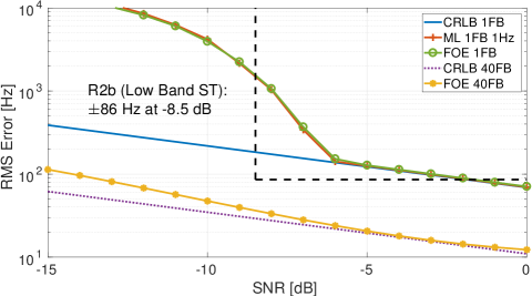
Figure 2: RMS frequency offset improvement by considering 40 FBs in a static channel. The CRLB is shown twice, once for a single FB and once with a 40 times larger receive power. The ML estimator is approximated using a $1\text{\,}\mathrm{Hz}$ resolution DFT.

III-B Multi-Frame Boundary Detection

The MFD is the first step in the synchronization process. Its main purpose is to estimate the start time of the MF, and therefore the position of the EC-SCH. One option is the use of ML ML estimator, like the one proposed in [9] for NB-IoT. However, the complexity of such an estimator scales with the maximum initial frequency offset and the number of correlated signals. For EC-GSM-IoT the FCCH and the training sequences of the SCH and EC-SCH are known a-priori and can be used for the search. Based on [9], we estimate the complexity for EC-GSM-IoT: Three different signals need to be cross-correlated with, and the maximum frequency offset is three times larger than in [9], resulting in a nine times larger real arithmetic complexity of $2.5\text{\,}\mathrm{GOP}\text{/}\mathrm{s}$. Storing the 9-bit correlation for $96$ frequency and $63\,750$ time offset candidates requires $55\text{\,}\mathrm{Mbit}$ of memory. This is clearly not suited for a low-power and low-cost implementation and we therefore propose a reduced complexity MFD algorithm.

The proposed MFD algorithm processes the received data in sliding windows of 200 symbols, which are offset by 50 symbols. The FOE procedure is re-used to look for the maximum spectral component in each window. The amplitude at this frequency, $C_{\text{FB}}[n]$, and the frequencies of the two highest components are stored. If the window contains FB FB, there is a high chance that one of these two frequencies corresponds to the sine. Since $1275$ windows, corresponding to one MF, are considered, $3825$ elements have to be stored in memory. Once an entire MF worth of samples has been received, the algorithm accumulates the five FB correlations for MF MF start in each window:

$$C_{\text{MF}}[n]=\sum\limits_{i=0}^{4}C_{\text{FB}}[n+250i\mod 1275].$$ (7)

Fig. 3 shows the two metrics in the noiseless case. Note that the normal bursts still result in a non-zero FB correlation.

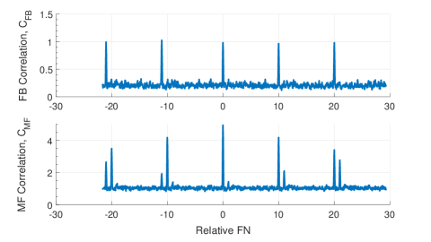
Figure 3: MFD: Correlation with the FBs and resulting MF correlation in ST ST channel without noise. The MF starts at $\text{FN}=0$.

The stored frequencies for the maximum of $C_{MF}$ are then compared. If there is a set of frequencies with a spread below an empirical threshold of $1\text{\,}\mathrm{kHz}$, the search is considered successful. Otherwise, additional MFs are searched and $C_{\text{MF}}$ is accumulated and the frequencies are updated. On a hit, the frequencies are also used as a coarse estimate of the frequency offset. At SNR SNR of $-8.5\text{\,}\mathrm{dB}$ in ST ST channel, the residual RMS frequency offset is $150\text{\,}\mathrm{Hz}$, which is sufficient to continue with decoding the EC-SCH.

One of the main challenges for the MFD is the structure of the GSM MF. The quasi-regular spacing of the FBs implies that the only difference between two MF starts is the location of a single FB. This results in a number of false side-peaks in the MF correlation, as can be seen in Fig. 3. This is especially problematic for fast fading channels, like the TU50 test case. We propose the use of the EC-SCH training sequences to find the actual start of the MF, since they follow a different repetition scheme. To this end, the MFD does not only return the peak of $C_{MF}$, but also the two positions 10 frames earlier and later as possible MF start candidates. The correct candidate is later found using the EC-SCH training sequences.

Fig. 4 shows the performance of the Spectrum MFD for the EC-GSM-IoT channels in the low and high bands. In order to allow the EC-SCH decoding sufficient time, the MFD is terminated after searching 4 MFs and the most likely candidate is used.

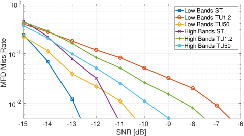
Figure 4: Spectrum MFD method miss rate for the EC-GSM-IoT channels. If none of the three candidates are within $\pm 80$ symbols of the MF start, the attempt is considered MFD MFD miss.

The MFD is the computationally most demanding part of the synchronization process. $5400$ windows need to be processed every second, each requiring a 256-point FFT. Including the calculation of the power and three-point interpolation, this results in an overall real arithmetic complexity of $40\text{\,}\mathrm{MOP}\text{/}\mathrm{s}$. This is suitable for a low-complexity hardware implementation and should result in a negligible power consumption, compared to the Radio Frequency (RF) receiver.

III-C Fine Time Offset Estimation and EC-SCH Decoding

Once the MFD is completed, the time offset is known to within $\pm 80$ symbols. In a next step, the accuracy has to be improved to $\pm 1$ symbol in order to decode the EC-SCH and fulfill Requirement R2a. This is done by cross-correlating the received EC-SCH training sequences with the known symbols. The time offsets in the range of the residual time offset of $\pm 80$ symbols are tried and the best match is selected. In a static channel at SNR SNR of $-8.5\text{\,}\mathrm{dB}$, the correct time offset is found in approximately $60\text{\,}\mathrm{\char 37\relax}$ of all attempts. Blind repetitions of the training sequences are thus received and the correlation outputs $K_{p}[\eta]$ are combined non-coherently:

$$\hat{\eta}=\mathop{\arg\max}_{\eta}K^{\prime}[\eta],\quad K^{\prime}[\eta]=\sum\limits_{p}|K_{p}[\eta]|^{2}.$$ (8)

Seven blind repetitions of the EC-SCH are sufficient to determine the correct time offset at SNR SNR of $-8.5\text{\,}\mathrm{dB}$ in ST ST channel. The correct MF start candidate is selected by choosing the one with the largest $K^{\prime}[\hat{\eta}]$ after $28$ blind repetitions have been received.

The last steps in the synchronization procedure are the fine frequency offset estimation and the decoding of the EC-SCH, which can be performed simultaneously. The EC-SCH decoding is started together with the fine time offset estimation and uses the most recent result of the latter. Seven repetitions of the EC-SCH are transmitted at the start of every MF and a total of 28 repetitions contain the same data. Repetitions in different MFs however, have different cyclic shifts, which depend on the frame number.

The actual decoding of the EC-SCH is implemented, as described in [5], where the Log-Likelihood Ratios for the EC-SCH repetitions are chase-combined for the four cyclic shift candidates. In-phase and Quadrature (IQ)-combination can significantly improve the channel estimation, especially when short training sequences are used. However, the EC-SCH uses longer training sequences and the phase between repetitions has to be estimated. Our simulations show that IQ-combination does not improve the performance of the decoder due to the phase estimation error at SNR SNR of $-8.5\text{\,}\mathrm{dB}$.

One option to detect the cyclic shift is comparing the data received in two successive MFs using a cross-correlation with lag $1$. Unfortunately, the correlation output is dominated by noise in the target SNR region, and this method fails. Alternatively, blind decoding attempts can be performed for all cyclic shifts, relying on the Cyclic Redundancy Check (CRC) checksum to filter out the invalid results. But this method also has a flaw, because the decoding attempts on invalid data can result in false positives from the checksum. The problem is further complicated by the relatively short CRC field length of 10 bits. If decoding is attempted after every received repetition, CRC false positives occur up to $19\text{\,}\mathrm{\char 37\relax}$ of the time. The proposed algorithm alleviates this problem by reducing the number of decoding attempts. In the low SNR region, a decoding attempt is only performed after $7N,N\geq 4$ repetitions have been received. This reduces the maximum false positive rate to $2.7\text{\,}\mathrm{\char 37\relax}$. It is below $1\text{\,}\mathrm{\char 37\relax}$ above $-8.5\text{\,}\mathrm{dB}$ SNR, which is acceptable and has to be handled after the synchronization.

IV Performance Evaluation

In order to evaluate the performance of the synchronization, we have performed simulations, where all the steps are performed in sequence. Fig. 5 shows the resulting overall miss rate for all of the channels specified for EC-GSM-IoT. $90\text{\,}\mathrm{\char 37\relax}$ of the simulations succeed at SNR SNR of $-11.5\text{\,}\mathrm{dB}$ in the low band ST channel and at SNR SNR of $-7.7\text{\,}\mathrm{dB}$ in the low band TU1.2 channel. This exceeds the 3GPP goals by $3\text{\,}\mathrm{dB}$ and $2.2\text{\,}\mathrm{dB}$, respectively. The Cumulative Distribution Function (CDF) for the synchronization time is shown in Fig. 6. It takes $1.6\text{\,}\mathrm{s}1.8\text{\,}\mathrm{s}$ to achieve $90\text{\,}\mathrm{\char 37\relax}$ successful synchronizations, meeting Requirement R1. The average synchronization time in ST ST channel at $-8.5\text{\,}\mathrm{dB}$ is $1.3\text{\,}\mathrm{s}$, corresponding to a $56\text{\,}\mathrm{\char 37\relax}$ reduction, compared to [5]. The MFD takes $250\text{\,}\mathrm{ms}425\text{\,}\mathrm{ms}$ on average, the rest of the time is spent receiving the EC-SCH. This is good from an energy standpoint, since the receiver can be turned off most of the time during the EC-SCH reception, recalling the MF structure in Fig. 1.

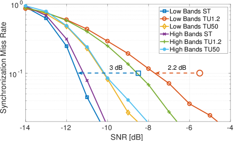
Figure 5: Synchronization miss rate for the different EC-GSM-IoT channels. A synchronization miss is either a timeout, or CRC CRC hit with incorrect data. The initial oscillator error is uniformly distributed between $\pm 25\text{\,}\mathrm{ppm}$.

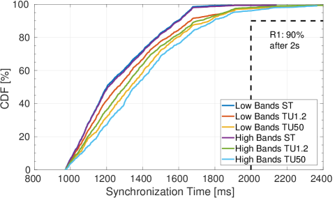
Figure 6: Synchronization time CDF at the ISL for EC-BCCH reference performance, assuming NF Noise Figure (NF) of $5\text{\,}\mathrm{dB}$. Unsuccessful synchronizations are counted towards to total.

Fig. 7 shows the fine time offset at the end of the synchronization process. It is below $\pm 1$ symbol in more than $99.5\text{\,}\mathrm{\char 37\relax}$ of the attempts for all the channels at the ISL for EC-SCH reference performance, which meets Requirement R2a. As shown in Fig. 8, the residual frequency offset after the fine FOE over 40 FBs is below $0.1\text{\,}\mathrm{ppm}$ in $99\text{\,}\mathrm{\char 37\relax}$ of the test cases, which meets Requirement R2b.

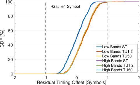
Figure 7: Residual time offset CDF at the ISL for EC-SCH reference performance, assuming NF NF of $5\text{\,}\mathrm{dB}$.

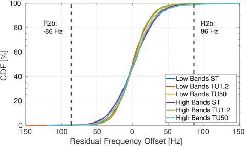
Figure 8: Residual frequency offset CDF at the ISL for EC-SCH reference performance, assuming NF NF of $5\text{\,}\mathrm{dB}$. Unsuccessful synchronizations are counted towards to total, but not shown.

V Cell Search

A cell search may have to be performed, whenever the device cannot reach BS BS at a known frequency. Then, it has to scan all $298+673$ potential low and high band BCCH carriers. Legacy GSM devices look for a suitable carrier by performing receive power measurements, which are not feasible below the noise floor. The duration of the cell search becomes problematic in EC-GSM-IoT, because the device must perform a partial synchronization to all potential carriers [10]. Like other cIoT standards, EC-GSM-IoT trades synchronization time for an improvement in coverage. As in [10], we propose the use of the MFD to detect the presence of GSM GSM carrier in extended coverage. Their algorithm requires 10 MFs to achieve a $99\text{\,}\mathrm{\char 37\relax}$ detection rate in TU TU$1.2$ channel. Our proposed algorithm can achieve the same performance after searching only 4 MFs. However, the limiting case is the high band TU50 channel with a maximum frequency offset of $\pm 50\text{\,}\mathrm{kHz}$. In this case, 7 MFs are required to achieve a $99\text{\,}\mathrm{\char 37\relax}$ detection rate. No false detections were simulated in $10\,000$ test cases. With this $30\text{\,}\mathrm{\char 37\relax}$ reduction compared to [10], the cell search takes $27$ minutes and a maximum of $113$ full cell searches are possible with a $5\text{\,}\mathrm{W}\text{\,}\mathrm{h}$ battery .

VI Conclusion

We have presented the first complete set of algorithms, which is able to successfully synchronize at SNR SNR as low as $-11.5\text{\,}\mathrm{dB}$. It fulfills the requirements for the synchronization time and the residual time and frequency offset with a low computational complexity. Our simulations show that it exceeds the 3GPP target by $3\text{\,}\mathrm{dB}$ in the best-case, resulting in MCL MCL of up to $170.5\text{\,}\mathrm{dB}$. In the worst-case the target is exceeded by $2.2\text{\,}\mathrm{dB}$, corresponding to MCL MCL of $166.7\text{\,}\mathrm{dB}$. The network synchronization supports a large frequency offset oscillator, enabling a low-cost EC-GSM-IoT implementation.

References

- [1] Release 13, 3GPP Std., Mar. 2016. [Online]. Available: http://www.3gpp.org/release-13
- [2] Nokia. (2017) IoT connectivity – understanding the options and choices. https://resources.ext.nokia.com/asset/201050.
- [3] H. Kröll et al., “Low-complexity frequency synchronization for GSM systems: Algorithms and implementation,” in Ultra Modern Telecommunications and Control Systems and Workshops (ICUMT), 2012 4th International Congress on, 2012, pp. 168–173.
- [4] U. S. Jha, “Acquisition of frequency synchronization for GSM and its evolution systems,” in Personal Wireless Communications, 2000 IEEE International Conference on. IEEE, 2000, pp. 558–562.
- [5] B. Weber et al., “A SAW-less RF-SoC for cellular IoT supporting EC-GSM-IoT -121.7dBm sensitivity through EGPRS2A 592kbps throughput,” in European Solid-State Circuits Conference (ESSCIRC), 2017.
- [6] Cellular System Support for Ultra Low Complexity and Low Throughput Internet of Things, 3GPP TR 45.820, Rev. 2.1.0, Aug. 2015. [Online]. Available: http://www.3gpp.org/DynaReport/45820.htm
- [7] D. Rife and R. Boorstyn, “Single tone parameter estimation from discrete-time observations,” IEEE Transactions on Information Theory, vol. 20, no. 5, pp. 591–598, 1974.
- [8] C. Yang and G. Wei, “A noniterative frequency estimator with rational combination of three spectrum lines,” IEEE Transactions on Signal Processing, vol. 59, no. 10, pp. 5065–5070, 2011.
- [9] H. Kröll et al., “Maximum-likelihood detection for energy-efficient timing acquisition in NB-IoT,” in Wireless Communications and Networking Conference Workshops (WCNCW). IEEE, 2017, pp. 1–5.
- [10] Intel Corp., “GP-160091: EC-FCCH design for quick and robust EC-GSM synchronization,” in TSG GERAN #69, Malta, Feb. 2016.