Dispersive shock wave theory for nonintegrable equations

Abstract

We suggest a method for calculation of parameters of dispersive shock waves in framework of Whitham modulation theory applied to non-integrable wave equations with a wide class of initial conditions corresponding to propagation of a pulse into a medium at rest. The method is based on universal applicability of Whitham’s ‘number of waves conservation law’ as well as on the conjecture of applicability of its soliton counterpart to the above mentioned class of initial conditions which is substantiated by comparison with similar situations in the case of completely integrable wave equations. This allows one to calculate the limiting characteristic velocities of the Whitham modulation equations at the boundary with the smooth part of the pulse whose evolution obeys the dispersionless approximation equations. We show that explicit analytic expressions can be obtained for laws of motion of the edges. The validity of the method is confirmed by its application to similar situations described by the integrable Korteweg-de Vries (KdV) and nonlinear Schrödinger (NLS) equations and by comparison with the results of numerical simulations for the generalized KdV and NLS equations.

I Introduction

It is well known that if one neglects effects of dissipation and dispersion, then the theory of propagation of nonlinear waves suffers from breaking singularity developed at some finite moment of time $t_{b}$ after which a formal solution of nonlinear wave equations becomes multi-valued. The classical approach to resolution of this problem is based physically on taking into account dissipation effects resulting in formation of shock waves instead of the non-physical multi-valued solutions. Since in practice the dissipation is often very small and, consequently, the width of shocks is very small, too, such shocks can be treated as surfaces of discontinuities of physical parameters whose values at both sides of such a surface are related by jump conditions derived from conservation of mass of the fluid, its momentum and energy LL-6 ; CF-50 . As a result, one arrives at remarkably powerful theory which has found numerous applications in science and technology.

However, in many physical systems the dissipative effects are relatively small compared with dispersion effects. The well-known example of such a situation is given by “undular bores” in shallow water waves theory (see, e.g., bl-54 ). In this case, interplay of relatively strong dispersion and weak dissipation leads to formation of a wide stationary oscillatory structure instead of a standard shock discontinuity. The generality of this situation was underlined by Sagdeev sagdeev who considered similar structures in plasma physics and quantitative asymptotic theory of such undular bores was developed by Johnson johnson-70 in framework of the Korteweg-de Vries-Burgers equation incorporating both damping and dispersion.

If the damping effects are measured by some parameter (say, the viscosity coefficient) $\nu$, then the asymptotic stationary stage is developed at very large time $t\gtrsim\nu^{-1}$, hence for considerable period $t\ll\nu^{-1}$ these damping effects can be neglected and the wave evolution is essentially non-stationary. In this case, short-wavelength nonlinear oscillations are generated after the wave breaking moment instead of a classical viscous shock discontinuity. Since such a non-stationary oscillatory structure describes transition between two different states of smooth flow, it is usually called dispersive shock wave (DSW). The simplest and, apparently, most powerful theoretical approach to description of DSWs was formulated by Gurevich and Pitaevskii gp-73 in framework of the Whitham theory of modulation of nonlinear waves whitham-65 ; whitham-74 which was based on large difference between scales of the wavelength of nonlinear oscillations within DSW and the size of the whole DSW. Further development of nonlinear physics demonstrated the generality of this phenomenon and now they have been observed in a number of physical situations (see, e.g., review article eh-16 and references therein).

Due to the above mentioned difference of time scales, the modulation parameters change slowly along the DSW and their evolution is governed by the Whitham equations which can be obtained by averaging of the conservation laws of the wave equation under consideration over fast oscillations within the DSW. Although this approach is very general, its practical applicability depends crucially on mathematical properties of the nonlinear wave equations which describe the evolution of the wave. The great achievement of Whitham was that in the case of waves whose evolution is described by the Korteweg-de Vries (KdV) equation he succeeded in transformation of the modulation equations to the so-called diagonal Riemann form. Gurevich and Pitaevskii used just this form of modulation equations in their seminal paper gp-73 . It became clear later ffml-80 , that Whitham’s diagonalization of the modulation equations was possible due to the special property, discovered in Ref. ggkm-67 , of complete integrability of the KdV equation. Development of the finite-gap integration method lax-74 ; nov-74 as well as of the methods of derivation ffml-80 ; krich-88 and solution tsarev ; dn-93 of the Whitham equations permitted one to extend the Gurevich-Pitaevskii approach to a number of other completely integrable equations of physical interest (see, e.g., eh-16 ). Complemented by the perturbation theory, derived for the KdV equation with small viscosity term added fml-84 ; akn-87 ; gp-88 ; mg-95 and later generalized to a wide class of perturbed completely integrable equations in Ref. kamch-04 , this theory has found many important applications.

On the contrary, development of the general Whitham method of modulations, not restricted to completely integrable equations, was much slower and its progress was quite limited. Apparently, the first general statement was made by Gurevich and Meshcherkin gm-84 , who proposed the condition which replaces the “jump conditions” known in the theory viscous shocks. This condition is formulated in terms of Riemann invariants of the hydrodynamic system obtained in the dispersionless limit of the original nonlinear wave equations under consideration. Typically, wave breaking occurs in the simple-wave flow when all physical variables of the system can be expressed as functions of only one of them what means that after transformation to the corresponding Riemann invariants only one of them breaks and the others remain constant. Gurevich and Meshcherkin claimed that this statement is correct also after formation of a DSW, so that flows at both its edges have the same values of the non-breaking Riemann invariants. This property is evidently correct in a simple case of self-similar solutions of Whitham equations for the KdV equation studied in Ref. gp-73 , when Whitham equations are transformed to the diagonal form, and Gurevich and Meshcherkin generalize it to situations when Riemann invariants of the modulation equations are unknown or even do not exist.

A remarkable contribution into the general Whitham theory of modulations was made by El el-05 who showed that in simple-wave DSWs of Gurevich-Meshcherkin type it is possible to find parameters of the DSW at its harmonic edge without full integration of the Whitham modulation equations by using instead the Whitham conservation of number of waves equation

$$\frac{\partial k}{\partial t}+\frac{\partial\omega(k)}{\partial x}=0,$$ (1)

where $k$ and $\omega$ are the wave vector and the frequency of a linear harmonic wave $\propto\exp[i(kx-\omega t)]$ propagating along a smooth background. El noticed that in the simple-wave breaking situation the physical parameters at the small-amplitude DSW edge depend on a single parameter only. As a result, Eq. (1) reduces to an ordinary differential equation which has an integral and the value of this integral can be found with the use of the Gurevich-Meshcherkin conjecture. This yields the value of the wave number of the wave packet at the small-amplitude edge of the DSW which allows one to calculate the speed of this edge equal to the group velocity of the wave packet provided the other parameters of the wave at this edge are also known.

The importance of the conservation of number of waves law (1) was underlined by Whitham whitham-65 ; whitham-74 who noticed that it is a direct consequence of definitions of the wave vector $k=\partial\theta/\partial x$ and the frequency $\omega=-\partial\theta/\partial t$ in a slowly modulated wave, where $\theta=\theta(x,t)$ is the phase of the wave. Therefore $k$ and $\omega$ are defined also for nonlinear waves and Eq. (1) fulfills along the entire DSW. As a result, it can be derived from any full system of modulation equations. Unfortunately, Eq. (1) loses its meaning at the soliton edge of a DSW where $k\to 0$. In spite of that, El showed el-05 that under some additional assumptions one can obtain from Eq. (1) the ordinary differential equation relating the physical variables along the characteristic of Whitham equations at the soliton edge of the DSW. Then one can get again the integral of this equation and find its value by the same Gurevich-Meshcherkin method. This procedure gives the inverse half-width $\widetilde{k}$ of the leading soliton and $\widetilde{k}$ is related to the soliton’s velocity by the well-known formula following from a simple reasoning: since a soliton propagates with the same velocity as its tails and if the tails of a soliton have an exponential form $\propto\exp[\mp\widetilde{k}(x-V_{s}t)]$, $x\to\pm\infty$, then the tails obey the same linearized equations which lead to the linear dispersion law $\omega=\omega(k)$. Hence, we arrive immediately at the statement that the soliton velocity $V_{s}$ is related with its inverse half-width $\widetilde{k}$ by the formula

$$V_{s}={\widetilde{\omega}(\widetilde{k})}/{\widetilde{k}},$$ (2)

where $\widetilde{\omega}(\widetilde{k})$ is defined as

$$\widetilde{\omega}(\widetilde{k})\equiv-i\omega(i\widetilde{k}).$$ (3)

This relationship was noticed long ago and helped a lot in finding soliton solutions of complicated systems of nonlinear wave equations (see, e.g., Refs. ai-77 ; dkn-03 ).

In an important particular case of initial step-like discontinuities all the parameters besides $k$ and $\widetilde{k}$ at the DSW edges are fixed, so after finding $k$ and $\widetilde{k}$ by the El method one can calculate such characteristics of the DSW as speeds of its edges and the leading soliton amplitude. Application of this scheme to the problems of evolution of initial step-like discontinuities for integrable equations, when the global solutions for the whole DSWs are known due to existence of Riemann invariants, showed that El’s method works perfectly well at least for this class of problems. Its further application to similar problems for non-integrable equations and comparison of the results with numerical simulations demonstrated its good applicability at least for moderate values of jumps of physical variables at the initial discontinuities. As a result, a number of interesting problems was successfully considered by this method (see, e.g., Refs. egs-06 ; egkkk-07 ; egs-09 ; ep-11 ; hoefer-14 ; ckp-16 ; hek-17 ; ams-18 ).

Obviously, ‘number of waves’ conservation equation (1) is universally correct for any DSWs beyond those generated from step-like initial discontinuities and indeed it was successfully used in estimate of asymptotic number of solitons generated from an initially localized pulse evolved according to non-integrable equation egs-08 (see also egkkk-07 ). However, El’s method cannot be applied directly to the problems of evolution of pulses different from step-like discontinuities and therefore it needs further development.

The aim of this paper is to develop the method of calculation of the main characteristics of DSWs generated in evolution of more general pulses than the initial step-like discontinuities. To this end, we study first whether Eq. (1) admits the transformation (3), so that the equation

$$\frac{\partial\widetilde{k}}{\partial t}+\frac{\partial\widetilde{\omega}(\widetilde{k})}{\partial x}=0$$ (4)

plays at the soliton edge the role analogous to that of Eq. (1). It is evident that, on the contrary to the situation with modulated nonlinear periodic wave, where wavelength has clear enough physical meaning along the DSW and $k$ can be defined as a gradient of the phase $\theta$, we cannot define in a similar way the inverse ‘wave width’ $\widetilde{k}$, so Eq. (4) has clear sense at the soliton edge only and even in this limit its correctness is not guaranteed. In spite of that, a simple calculation shows that it is correct in the case of integrable equations at the edge matching to the smooth profile of the pulse provided the initial profile belongs to the class of simple waves which means physically that the pulse propagates through medium ‘at rest’ with constant waves of the dispersionless Riemann invariants. Following to Gurevich and Meshcherkin gm-84 , we generalize this observation to non-integrable equations. As a result, the conditions of applicability of Eq. (4) are formulated in terms of dispersionless wave breaking patterns and mean physically that the wave breaking occurs at the boundary with the medium at rest. Naturally, these conditions are fulfilled for the step-like discontinuities, hence El’s theory is included into this approach.

Assuming correctness of Eq. (4), we can transform it again in vicinity of the soliton edge of the DSW to the ordinary differential equation in simple-wave type problems, and then this equation can be solved if an appropriate boundary condition at the small-amplitude edge is known in the problem under consideration. To find the law of motion of DSW’s edge at the boundary with the smooth dispersionless flow, we use the fact that in this limit the characteristic velocities of the Whitham equations have known values what allows one to write down the corresponding limiting Whitham equation in the hodograph transformed form and to solve it with the use of the fact that the smooth dispersionless solution is also known. This procedure generalizes to non-integrable equations the method used in Ref. gkm-89 for calculation of the law of motion of the small-amplitude edge in the KdV equation theory and applied recently in Ref. kamch-18 to calculation of the motion of the soliton edge at the boundary with the smooth solution in the nonlinear Schrödinger (NLS) equation theory.

Although in the case of monotonous initial pulses this method gives velocity of the edge at the boundary with smooth non-uniform distribution only, in the case of non-monotonous pulse the method provides also the asymptotic value of velocity of the opposite edge at the boundary with the medium at rest. Comparison of the results obtained by this method with known solutions of integrable KdV and NLS equations as well as with the results of numerical solution of non-integrable equations confirms its validity. Thus, the method greatly increases the area of applicability of the Whitham theory to description of evolution of DSWs in nonlinear wave systems. In particular, it can be applied to description of DSWs observed in experiments on evolution of pulses in shallow water waves hs-78 ; tkco-16 , nonlinear optics wkf-07 ; Fat14 ; Xu17 , Bose-Einstein condensates hoefer-06 ; ea-07 ; chang-08 .

The paper has the following structure. In Sec. II we discuss applicability of Eqs. (1) and (4) to the edges of DSWs for integrable KdV and NLS equations and formulate the conditions of applicability of Eq. (4) to non-integrable equations. The method formulated here is applied to different types of nonlinear wave equations in Sec. III and situations with uni-directional and two-directional propagation are considered separately in Secs. III.1 and III.2, respectively. In both cases, we show that our method reproduces correctly the known results obtained earlier for integrable KdV and NLS equations and then apply the method to typical in nonlinear physics generalized KdV and NLS equations. In Sec. IV the method is validated by comparison of analytical formulas obtained in Whitham approximation with exact numerical solution of the generalized NLS equation. Section V is devoted to conclusion and general discussion. Derivation of convenient for us form of El’s equations is given in the Appendix.

II Harmonic and soliton dispersion laws

We shall call the functions $\omega=\omega(k)$ and $\widetilde{\omega}=\widetilde{\omega}(\widetilde{k})$, which appear in Eqs. (1) and (4), as “harmonic” and “soliton” dispersion laws, respectively. As was indicated in the Introduction, these functions are defined by linearized equations of motion for small-amplitude (harmonic) and soliton’s tails limits, correspondingly, and they can be converted one into another by means of Eq. (3). To formulate the conditions of applicability of Eqs. (1) and (4) along DSW, we have to define $k$ and $\widetilde{k}$ in the vicinity of DSW edges which can be done if the periodic and soliton solutions of the equation under consideration are known. Moreover, if these solutions are parameterized by the Riemann invariants of the corresponding Whitham modulation equations, then we can check the validity of Eqs. (1) and (4) in the Whitham approximation. We shall make such a check at the small-amplitude and soliton edges of DSWs described by the KdV and NLS equations, and the results obtained will permit us to formulate a plausible conjecture about the conditions of applicability of Eq. (4).

II.1 KdV equation case and generalizations

As is well known (see, e.g., kamch2000 ), the KdV equation

$$u_{t}+6uu_{x}+u_{xxx}=0$$ (5)

has a periodic solution which can be written in the form

$$u(x,t)=r_{2}+r_{3}-r_{1}-2(r_{2}-r_{1})\mathrm{sn}^{2}(\sqrt{r_{3}-r_{1}}\,(x-Vt),m),$$ (6)

where

$$V=2(r_{1}+r_{2}+r_{3}),\qquad m=\frac{r_{2}-r_{1}}{r_{3}-r_{1}}$$ (7)

and $\mathrm{sn}$ is the Jacobi elliptic function. In the strictly periodic case the parameters $r_{1}\leq r_{2}\leq r_{3}$ are constant, but in slowly modulated waves they become slow functions of $x$ and $t$ whose evolution is governed by the Whitham equations

$$\frac{\partial r_{i}}{\partial t}+v_{i}(r_{1},r_{2},r_{3})\frac{\partial r_{i}}{\partial x}=0,\quad i=1,2,3,$$ (8)

where the expressions for the characteristic velocities $v_{i}(r)$ were obtained by Whitham whitham-65 ; whitham-74 (see also kamch2000 ).

In the small-amplitude limit $r_{2}-r_{1}\ll|r_{2}|$ the solution (6) transforms into a harmonic wave

$$\begin{split}&u(x,t)=r_{3}+(r_{2}-r_{1})\cos[2\sqrt{r_{3}-r_{1}}\,(x-Vt)],\\ &V=2(2r_{1}+r_{3}),\end{split}$$ (9)

and in this limit the Whitham velocities are equal to

$$v_{1}|_{r_{2}=r_{1}}=v_{2}|_{r_{2}=r_{1}}=12r_{1}-6r_{3},\quad v_{3}|_{r_{2}=r_{1}}=6r_{3}.$$ (10)

The harmonic dispersion law follows immediately from linearized Eq. (5),

$$\omega(k)=6uk-k^{3},$$ (11)

and it agrees with the expressions for $k$ and $\omega$ that follow from (9),

$$\begin{split}&k=2\sqrt{r_{3}-r_{1}},\\ &\omega=kV=4(2r_{1}+r_{3})\sqrt{r_{3}-r_{1}},\end{split}$$ (12)

if one takes into account that $u\approx r_{3}$ at this edge. Supposing that $r_{1}$ and $r_{3}$ evolve here according to the Whitham equations

$$\frac{\partial r_{1}}{\partial t}+(12r_{1}-6r_{3})\frac{\partial r_{1}}{\partial x}=0,\qquad\frac{\partial r_{3}}{\partial t}+6r_{3}\frac{\partial r_{3}}{\partial x}=0,$$ (13)

we readily find that the $k$ and $\omega$ defined by Eqs. (12) satisfy Eq. (1) identically. This agrees with the general statement that the number of waves conservation law (1) is a strict consequence of the Whitham modulation equations.

In a similar way, in the soliton limit $r_{2}\to r_{3}$ Eq. (6) reduces to the soliton solution

$$\begin{split}&u(x,t)=r_{1}+\frac{2(r_{3}-r_{1})}{\cosh^{2}[\sqrt{r_{3}-r_{1}}(x-V_{s}t)]},\\ &V_{s}=2(r_{1}+2r_{3}),\end{split}$$ (14)

and the Whitham velocities are given by the formulas

$$v_{1}|_{r_{2}=r_{3}}=6r_{1},\quad v_{2}|_{r_{2}=r_{3}}=v_{3}|_{r_{2}=r_{3}}=2r_{1}+4r_{3}.$$ (15)

Now the soliton dispersion law reads

$$\widetilde{\omega}(\widetilde{k})=6u\widetilde{k}+\widetilde{k}^{3}$$ (16)

and from Eq. (14) we get $u\approx r_{1}$ and

$$\begin{split}&\widetilde{k}=2\sqrt{r_{3}-r_{1}},\\ &\widetilde{\omega}=\widetilde{k}V_{s}=4(r_{1}+2r_{3})\sqrt{r_{3}-r_{1}}.\end{split}$$ (17)

Substitution of these expression into Eq. (4) with account of the Whitham equations

$$\frac{\partial r_{1}}{\partial t}+6r_{1}\frac{\partial r_{1}}{\partial x}=0,\qquad\frac{\partial r_{3}}{\partial t}+(2r_{1}+4r_{3})\frac{\partial r_{3}}{\partial x}=0$$ (18)

yields after simple transformations the equation

$$\frac{\partial\widetilde{k}}{\partial t}+\frac{\partial\widetilde{\omega}(\widetilde{k})}{\partial x}=4\widetilde{k}\frac{\partial r_{3}}{\partial x}.$$ (19)

Hence, Eq. (4) does not hold for DSWs with changing Riemann invariant $r_{3}$ in the vicinity of the soliton edge. However, as is known from Gurevich-Pitaevskii theory gp-73 for evolution of the initial step-like discontinuity, in this particular case $r_{3}=\mathrm{const}$ and for such a DSW Eq. (4) is fulfilled. This type of DSWs corresponds to the diagram of Riemann invariants shown in Fig. 1. Schematically, this diagram is equivalent to a formal multi-valued solution of the Hopf equation,

$$u_{t}+6uu_{x}=0,$$ (20)

which is the dispersionless approximation of the KdV equation, for the problem with the initial step-like discontinuity, where $r_{1},r_{2},r_{3}$ symbolize the three values of this multi-valued solution. (To avoid any confusion, we stress that numerically the parameter $u$ in the formal dispersionless solution differs from values of $r_{2}$ obtained in the solution of the Whitham equations, and the same difference exists between the coordinates $x_{L},\,x_{R}$ of the edges in these two situations, that is we mean here just qualitative geometric similarity of the respective diagrams rather than their quantitative numerical identity.) It is natural to suppose that Eq. (4) remains correct for DSWs described by non-integrable wave equations for some variable $u$, if the corresponding dispersionless wave breaking pattern is given geometrically by Fig. 1, although its counterpart for the Riemann invariants of Whitham equations does not exist anymore. Actually, this conjecture corresponds exactly to the El theory el-05 applied to the step-like initial problems.

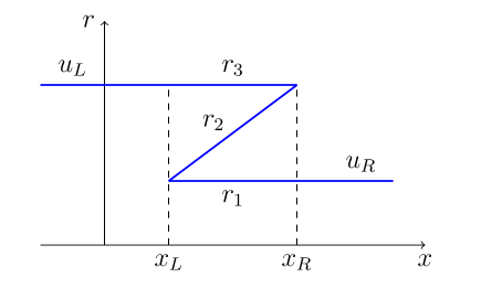
Figure 1: Plots of Riemann invariants for the solution of the step-like initial problem. In this case $r_{3}=\mathrm{const}$ and Eq. (4) is correct.

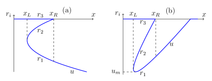
Figure 2: Plots of Riemann invariants for wave breaking of “negative” pulses with monotonous (a) and localized (b) profiles. In both cases $r_{3}=\mathrm{const}$ and Eq. (4) is correct.

Now we notice that there exist other situations shown in Fig. 2 where $r_{3}=\mathrm{const}$ in the integrable KdV equation theory, whereas both $r_{1}$ and $r_{2}$ change with time and space coordinate. The corresponding solutions of the Whitham equations were called quasi-simple in Ref. gkm-89 . We distinguish here the cases with monotonous and non-monotonous initial pulses to underline that a non-monotonous initial pulse $u=u_{0}(x)$ is characterized also by some minimal value $u_{m}$ which plays an important role at the asymptotic stage of evolution of the DSW evolved from such a pulse. In this type of DSWs, the soliton edge $x_{R}$ propagates along a non-uniform and time-dependent background evolving from $u_{0}(x)$, and the law of motion of this edge can be found with the use of Eq. (4) bypassing the global solution of the full system of Whitham equations. Again it is natural to assume that this method can be extended to non-integrable equations, if the wave breaking pattern for a single wave variable $u$ has the same geometric form and the dispersion and nonlinearity are such that the soliton edge is located at the boundary with the dispersionless smooth solution.

On the contrary, if the wave breaking pattern has the form depicted in Fig. 3, then $r_{3}$ is not constant, Eq. (4) loses its applicability and the law of motion of the soliton edge $x_{R}$ cannot be found by solving this equation. It is known that such a localized positive pulse evolves asymptotically into a sequence of well-separated solitons and in the KdV equation case the velocity of the leading soliton can be found with the use of the Karpman formula karpman-68 . The number of solitons generated from the initial pulse can be calculated in the non-integrable case by the method of Refs. egkkk-07 ; egs-08 . The universal Eq. (1) is always correct and, as we shall see, permits one to find the law of motion of the small-amplitude edge $x_{L}$. To distinguish these two situations, we shall call them “negative” in the case of Fig. 2 and “positive” in the case of Fig. 3. It is important for us that for a proper relative sign of nonlinear and dispersive effects, in the first case the soliton edge is located at the boundary $x_{R}$ with the smooth solution $u$ and in the second case the small-amplitude edge is located at such a boundary $x_{L}$.

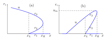
Figure 3: Plots of Riemann invariants for wave breaking of “positive” pulses with monotonous (a) and localized (b) profiles. In both cases $r_{3}$ changes with $x$ and Eq. (4) is not applied.

At the same time we should notice that although Eq. (1) is always applicable, in situations shown in Fig. 2 the small-amplitude edge propagates into the region with constant $u$ which is a trivial solution of the Hopf equation (20), that is there is no explicit relationship between the values of $u_{L}$, $x_{L}$ and $t$ at the small-amplitude edge. Therefore the law of motion of this edge cannot be found by the method suggested here. In spite of that, in the case of an initially localized pulse depicted in Fig. 2(b), the asymptotic value of the velocity of the small-amplitude edge can be expressed in terms of the minimal value $u_{m}$ of the initial distribution. All these problems will be considered in Sec. III.

II.2 NLS equation case and generalizations

Now we turn to the question of validity of Eq. (4) for DSWs whose evolution is described by the NLS equation

$$i\psi_{t}+\frac{1}{2}\psi_{xx}-|\psi|^{2}\psi=0.$$ (21)

In this case it is convenient to represent the periodic solution in terms of the variables $\rho$ and $u$ such that

$$\psi(x,t)=\sqrt{\rho(x,t)}\exp\left(i\int^{x}u(x^{\prime},t)dx^{\prime}\right).$$ (22)

Then, for example, in the physical context of Bose-Einstein condensates, $\rho$ has a meaning of its density and $u$ of its flow velocity. In terms of these variables, the NLS equation can be written as a system of hydrodynamics-like equations

$$\begin{split}&\rho_{t}+(\rho u)_{x}=0,\\ &u_{t}+uu_{x}+\rho_{x}+\left(\frac{\rho_{x}^{2}}{8\rho^{2}}-\frac{\rho_{xx}}{4\rho}\right)_{x}=0,\end{split}$$ (23)

where the last term in the second equations describes the dispersion effects. In smooth flows, when higher derivatives are small, this term can be neglected and we arrive at the dispersionless limit represented by the ‘shallow water equations’

$$\rho_{t}+(\rho u)_{x}=0,\quad u_{t}+uu_{x}+\rho_{x}=0.$$ (24)

The periodic solution of the system (23) is given by the formulas (see, e.g., kamch2000 )

$$\begin{split}\rho(x,t)=&\tfrac{1}{4}(r_{4}-r_{3}-r_{2}+r_{1})^{2}+(r_{4}-r_{3})(r_{2}-r_{1})\\ &\times\mathrm{sn}^{2}(\sqrt{(r_{4}-r_{2})(r_{3}-r_{1})}(x-Vt),m),\\ u(x,t)=&V+\frac{j}{\rho(x,t)},\end{split}$$ (25)

where

$$\begin{split}V=&\frac{1}{2}(r_{1}+r_{2}+r_{3}+r_{4}),\quad m=\frac{(r_{2}-r_{1})(r_{4}-r_{3})}{(r_{4}-r_{2})(r_{3}-r_{1})},\\ j=&\frac{1}{8}(-r_{1}-r_{2}+r_{3}+r_{4})(-r_{1}+r_{2}-r_{3}+r_{4})\\ &\times(r_{1}-r_{2}-r_{3}+r_{4}),\end{split}$$ (26)

that is $j$ has the meaning of the density current in the reference frame where the phase velocity $V$ is equal to zero. The parameters $r_{1}\leq r_{2}\leq r_{3}\leq r_{4}$ play the role of the Riemann invariants in a modulated wave so that the Whitham equations have a diagonal form

$$\frac{\partial r_{i}}{\partial t}+v_{i}(r)\frac{\partial r_{i}}{\partial x}=0,\quad i=1,2,3,4,$$ (27)

and expressions for the velocities $v_{i}$ were found in Refs. FL-87 ; pavlov-87 . At the small-amplitude edge $r_{3}=r_{4}$ we have a harmonic wave

$$\begin{split}\rho=&\frac{1}{4}(r_{2}-r_{1})^{2}-\frac{1}{2}(r_{2}-r_{1})(r_{4}-r_{3})\\ &\times\cos\left[2\sqrt{(r_{4}-r_{1})(r_{4}-r_{2})}(x-Vt)\right],\\ V=&\frac{1}{2}(r_{1}+r_{2}+2r_{4}),\end{split}$$ (28)

and the velocities $v_{i}$ are given here by

$$\begin{split}&v_{1}=\frac{1}{2}(3r_{1}+r_{2}),\quad v_{2}=\frac{1}{2}(r_{1}+3r_{2}),\\ &v_{3}=v_{4}=2r_{4}-\frac{(r_{2}-r_{1})^{2}}{2(2r_{4}-r_{1}-r_{2})}.\end{split}$$ (29)

(Analogous formulas can be obtained in another small-amplitude limit $r_{2}=r_{1}$, but we shall not need them in what follows.) At the soliton edge we have the dark soliton solution

$$\begin{split}&\rho=\frac{1}{4}(r_{4}-r_{1})^{2}-\frac{(r_{4}-r_{2})(r_{2}-r_{1})}{\cosh^{2}[\sqrt{(r_{4}-r_{2})(r_{2}-r_{1})}(x-V_{s}t)]},\\ &V_{s}=\frac{1}{2}(r_{1}+2r_{2}+r_{4}),\end{split}$$ (30)

and near the soliton edge the characteristic velocities of the Whitham system are given by the formulas

$$\begin{split}&v_{1}=\frac{1}{2}(3r_{1}+r_{4}),\quad v_{2}=v_{3}=\frac{1}{2}(r_{1}+2r_{2}+r_{4}),\\ &v_{4}=\frac{1}{2}(r_{1}+3r_{4}).\end{split}$$ (31)

Now we can check the validity of Eqs. (1) and (4) in framework of the Whitham theory for the NLS equation.

At the small-amplitude edge Eq. (28) gives the expressions for the wave vector and the frequency,

$$\begin{split}&k=2\sqrt{(r_{4}-r_{1})(r_{4}-r_{2})},\\ &\omega=kV=(r_{1}+r_{2}+2r_{4})\sqrt{(r_{4}-r_{1})(r_{4}-r_{2})}.\end{split}$$ (32)

Their substitution into Eq. (1) with account of the Whitham equations (27) with velocities (29) demonstrate after simple calculation that Eq. (1) is fulfilled identically. [Similar calculation proves the validity of Eq. (1) in another small-amplitude limit $r_{2}=r_{1}$.] Thus, we have confirmed again that the number of waves conservation law is a consequence of the Whitham equations in agreement with the general statement of Whitham whitham-65 ; whitham-74 .

At the soliton edge we find from Eq. (30) that

$$\begin{split}&\widetilde{k}=2\sqrt{(r_{4}-r_{1})(r_{4}-r_{2})},\\ &\widetilde{\omega}=(r_{1}+2r_{2}+r_{4})\sqrt{(r_{4}-r_{1})(r_{4}-r_{2})},\end{split}$$ (33)

and substitution of these expressions into Eq. (1) with account of Whitham equations (27) with velocities (31) gives

$$\frac{\partial\widetilde{k}}{\partial t}+\frac{\partial\widetilde{\omega}(\widetilde{k})}{\partial x}=2\widetilde{k}\frac{\partial r_{2}}{\partial x}.$$ (34)

Here we should make an important remark. In the above expressions for the soliton limit we denoted the common value of the two Riemann invariants $r_{3}=r_{2}$ as $r_{2}$ which explains the appearance of $r_{2}$ in the right-hand side of Eq. (34). If we had denoted it as $r_{3}$, then we would have obtained Eq. (34) with $r_{2}$ replaced by $r_{3}$. This restores the two-directional symmetry of the NLS equation.

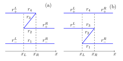
Figure 4: Diagrams of Riemann invariants for wave breaking of step-like pulses in NLS equation theory.

Thus, we arrive at the conclusion that Eq. (1) is universally correct and (4) is correct when in the corresponding diagram of Riemann invariants we have either $r_{2}$ or $r_{3}$ constant. Obviously, this takes place, for example, in the diagrams shown in Fig. 4, where $r_{i}$ ($i=1,2,3,4$) denote the Riemann invariants of of the Whitham equations and $r_{\pm}^{L}$, $r_{\pm}^{R}$ denote the Riemann invariants

$$r_{\pm}=\frac{u}{2}\pm\sqrt{\rho}$$ (35)

of the dispersionless system (24) which takes a diagonal Riemann form in terms of these variables,

$$\begin{split}&\frac{\partial r_{+}}{\partial t}+v_{+}(r_{+},r_{-})\frac{\partial r_{+}}{\partial x}=0,\\ &\frac{\partial r_{-}}{\partial t}+v_{-}(r_{+},r_{-})\frac{\partial r_{-}}{\partial x}=0,\end{split}$$ (36)

where

$$\begin{split}&v_{+}(r_{+},r_{-})=\frac{1}{2}(3r_{+}+r_{-}),\\ &v_{-}(r_{+},r_{-})=\frac{1}{2}(r_{+}+3r_{-}).\end{split}$$ (37)

These velocities coincide exactly with the corresponding limits of the Whitham velocities which provides continuous matching of the Riemann invariants of Whitham and dispersionless equations as is shown in Fig. 4.

The diagrams shown in Fig. 4 symbolize the step-like wave breaking of simple waves, so that in Fig. 4(a) the invariant $r_{+}$ of the right-propagating wave breaks and $r_{-}$ is constant whereas in Fig. 4(b) the invariant $r_{-}$ of the left-propagating wave breaks and $r_{+}$ remains constant. The Gurevich-Mescherkin conjecture claims that even if the Riemann invariants of the Whitham modulation equations do not exist, nevertheless the values of the dispersionless Riemann invariant $r_{-}$ is transferred through the DSW generated after wave breaking of the right-propagating simple wave and, in a similar way, the value of $r_{+}$ is transferred through the DSW generated after the wave breaking of the left-propagating wave. El’s theory el-05 corresponds to this situation and provides the method of calculation of parameters of the edges of DSWs generated from initial step-like discontinuities for the non-integrable wave equations case. The agreement of El’s theory with numerical simulations shows that although the invariants $r_{2}$ or $r_{3}$ do not exist along the whole DSW, their existence at its edges ($r_{2}=r_{+}^{R}$ in Fig. 4(a) or $r_{3}=r_{-}^{L}$ in Fig. 4(b)) is enough for finding the velocities of DSW edges in the case of step-like initial problems. Here we assume correctness of Eq. (4) in vicinity of the DSW edge. Actually, this statement means generalization of the Gurevich-Mescherkin conjecture to quasi-simple waves where either $r_{\pm}^{L}$ or $r_{\pm}^{R}$ are constant at one of the edges of the DSW. As is clear from Eqs. (35), in the NLS equation case the constancy of both dispersionless Riemann invariants at one of the edges of the DSW means that this DSW propagates into a uniform ($\rho_{0}=\mathrm{const}$) region with constant flow velocity ($u_{0}=\mathrm{const}$) which can be put equal to zero in the appropriate reference frame. We can formulate these observations as a conjecture that Eq. (4) holds for DSWs propagating into uniform ‘quiescent’ medium.

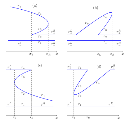
Figure 5: Diagrams of Riemann invariants for wave breaking of “positive” pulses with monotonous (a) and localized (b) profiles of dispersionless Riemann invariant $r_{+}$. In both cases $r_{2}=\mathrm{const}$ and Eq. (4) is correct. For “negative” initial distributions (c) and (d) of the invariant $r_{+}$ the invariants $r_{2}$ and $r_{3}$ of the Whitham modulation system vary with $x$ and Eq. (4) is not fulfilled.

Now we notice that, as in the KdV equation case, there exist other situations in the NLS equation theory where $r_{2}$ or $r_{3}$ are constant. In Fig. 5(a,b) the Riemann invariant $r_{+}$ with “positive” initial distribution breaks and we distinguish again here monotonous and localized pulses; in Fig. 5(c,d) we have depicted analogous situations with breaking of $r_{+}$-invariant for “negative” initial profiles. We have shown recently in Ref. kamch-18 that in the case corresponding to Fig. 5(a) the law of motion of the soliton edge $x_{L}(t)$ can be found without knowing the global solution of the Whitham equations. It is natural to suppose that this method can be generalized in such a way that the law of motion of the soliton edge can be found with the use of Eq. (4) for pulses whose evolution is governed by non-integrable wave equations, if the wave breaking patterns of the dispersionless Riemann invariants coincide geometrically with those shown in Fig. 5(a,b) in spite of that the Riemann invariants of the Whitham modulation equations do not exist anymore. Due to universal applicability of Eq. (1), the laws of motion of the small-amplitude edges at the boundaries with smooth solutions for breaking Riemann invariants can be found in situations whose integrable counterparts are depicted in Figs. 5(c,d) where $r_{2}$ and $r_{3}$ are not constant. In these cases, the small-amplitude edges $x_{R}$ propagate into smooth distributions of the dispersionless Riemann invariants $r_{+}$. The laws of motion of the soliton edges $x_{L}$ can be found only at the asymptotic stage of evolution, when the initial pulse evolves into a sequence of well separated solitons. In integrable cases this stage can be studied with the use of the Bohr-Sommerfeld quantization rule for the associated Lax spectral problem (see, e.g., kku-02 ) and in non-integrable cases the number of solitons can be calculated by the method suggested in Refs. egkkk-07 ; egs-08 .

Now, after formulation of the class of problems where the number of waves conservation law (1) and its soliton counterpart (4) are applicable, we can proceed to demonstration of their concrete applications to DSWs evolutions.

III Motion of dispersive shock edges

Evolution of DSWs generated from initial step-like discontinuities were studied in much detail in Refs. el-05 ; egs-06 ; egkkk-07 ; egs-09 ; ep-11 ; hoefer-14 ; ckp-16 ; hek-17 ; ams-18 by El’s method and we shall not consider this particular case here. Instead, we shall turn to the class of problems referred to in Ref. gkm-89 as quasi-simple DSWs. To illustrate the correctness of our approach, we shall consider first integrable situations where our results can be compared with the results known from solutions obtained by the inverse scattering transform method.

To simplify exposition, we notice here that El’s method together with the Gurevich-Meshcherkin conjecture can be formulated as an ‘extrapolation’ procedure, that is, instead of speaking about solving Eqs. (1) and (4) along edge characteristics of the Whitham system with the Gurevich-Meshcherkin initial condition, we say that we extrapolate solutions of the limiting Whitham equation (1) or (4) from the vicinity of one edge to the whole DSW and impose the proper boundary condition at the opposite edge. This formulation gives the same results as El’s method and has some advantages for generalizations of the method to non-step-like initial conditions.

III.1 Unidirectional propagation

We suppose that our nonlinear wave is described by a single variable $u$. To illustrate the method, we consider first the completely integrable KdV equation, but we shall use here only the general properties of the Whitham modulation equations not related with their explicit diagonal form.

III.1.1 KdV equation: Positive pulse

We shall start with a monotonous pulse with the initial form $u_{0}(x)>0$ shown in Fig. 3(a). Our task here is to find the law of motion of the small-amplitude edge $x_{L}(t)$. In the region $x<x_{L}(t)$ the pulse is smooth and its evolution is described by the dispersionless Hopf equation (20) whose solution reads

$$x-6ut={\overline{x}}(u),$$ (38)

where ${\overline{x}}(u)$ is a function inverse to $u_{0}(x)$. On the other hand, the function $u(x)$ can be treated at $x=x_{L}$ as a solution of the Whitham equations in the limit $x\to x_{L}+0$ corresponding to the characteristic velocity $v_{+}=6\overline{u}$ of the Whitham system, where $\overline{u}$ is understood as a mean value of the wave variable at this small-amplitude limit. But, according to the general principles of the Whitham theory whitham-65 ; whitham-74 , the system of Whitham modulation equations has in this limit another characteristic velocity $v_{-}$ equal to the group velocity

$$v_{-}=\frac{dx_{L}}{dt}=\frac{d\omega}{dk}=6\overline{u}-3k^{2}$$ (39)

of the small-amplitude wave at the edge $x_{L}$. The wave vector $k$ and the frequency $\omega$ change at this edge in such a way that Eq. (1) is fulfilled,

$$\frac{\partial k}{\partial t}+\frac{\partial\omega}{\partial x}=0,\qquad\omega(\overline{u},k)=6\overline{u}k-k^{3}.$$ (40)

If we suppose that we deal here with a simple-wave type of solutions of the Whitham system, which agrees with the form (38) of the smooth solution, then $k$ depends on $x$ and $t$ via $\overline{u}(x,t)$, $k=k(\overline{u})$. Taking into account that at this edge Eq. (20) holds, we reduce Eq. (40) to an ordinary differential equation

$$k\frac{dk}{d\overline{u}}=2.$$ (41)

Now we solve this equation and extrapolate the solution to the whole DSW with the boundary condition that at the opposite soliton edge the distance between solitons tends to infinity,

$$k=0\qquad\text{at}\qquad\overline{u}=0.$$ (42)

This extrapolation gives a correct value

$$k=2\sqrt{u}$$ (43)

of the wave number at the edge $x_{L}(t)$ where $u={\overline{u}}$. Actually, this procedure is equivalent to solving the El equation el-05 , but we prefer to use here directly the number of waves conservation law Eq. (40) to make the method more transparent and flexible for further generalizations.

Substitution of Eq. (43) into Eq. (39) gives the value of the characteristic velocity

$$v_{-}=\frac{dx_{L}}{dt}=-6u,$$ (44)

which corresponds to the limiting form of the Whitham equation

$$\frac{\partial x_{L}}{\partial u}+6u\frac{\partial t}{\partial u}=0$$ (45)

written in the hodograph transform representation (see, e.g., kamch2000 ). This equation must be compatible with Eq. (38) taken at $x=x_{L}$, so that elimination of $x_{L}$ yields the differential equation

$$2u\frac{dt}{du}+t=-\frac{1}{6}\frac{d{\overline{x}}}{du}.$$ (46)

We suppose that wave breaking occurs at the moment $t=0$ at the boundary $u=0$ of the initial pulse. Hence, Eq. (46) must be solved with the initial condition

$$t(0)=0$$ (47)

which gives at once

$$t(u)=-\frac{1}{12\sqrt{u}}\int_{0}^{u}\frac{{\overline{x}}^{\prime}(u)}{\sqrt{u}}\,du$$ (48)

and substitution of this expression into Eq. (38) yields

$$x_{L}(u)=-\frac{\sqrt{u}}{2}\int_{0}^{u}\frac{{\overline{x}}^{\prime}(u)}{\sqrt{u}}\,du+{\overline{x}}(u).$$ (49)

It is assumed here (and in similar situations in what follows) that the function ${\overline{x}}(u)$ vanishes in the limit $u\to 0$ fast enough so that the integrals converge and tend to zero in this limit to fulfill the initial condition (47). The formulas (48) and (49) give us the law of motion of the small-amplitude edge $x_{L}(t)$ in parametric form for a positive monotonous profile $u_{0}(x)$ of the initial pulse. For example, in the case of a parabolic profile $u_{0}(x)=\sqrt{-x}$, we have ${\overline{x}}(u)=-u^{2}$, and easy calculation reproduces the well-known result gkm-89 ; ks-90 (see also kamch2000 )

$$x_{L}(t)=-27t^{2}.$$ (50)

Our approach can be considered as a modification of calculation presented in Ref. gkm-89 , but, instead of using the known expression for the characteristic velocity $v_{-}$ in terms of Riemann invariants, we have calculated it in Eq. (44) by means of El’s rule which is applicable equally to both integrable and non-integrable wave equations.

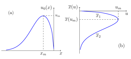
Figure 6: (a) Initial profile $u_{0}(x)$ of a localized pulse. (b) The inverse function ${\overline{x}}(u)$ is represented by two branches ${\overline{x}}_{1}(u)$ and ${\overline{x}}_{2}(u)$.

In the case of a localized initial pulse Fig. 6(a), the inverse function becomes two-valued and we denote its two branches as ${\overline{x}}_{1}(u)$ and ${\overline{x}}_{2}(u)$ (see Fig. 6(b)). The formulas (48) and (49) remain true up to the moment

$$t_{m}=-\frac{1}{12\sqrt{u_{m}}}\int_{0}^{u_{m}}\frac{{\overline{x}}^{\prime}_{1}(u)}{\sqrt{u}}\,du$$ (51)

at which the small-amplitude edge reaches the coordinate

$$x_{m}=-\frac{\sqrt{u_{m}}}{2}\int_{0}^{u_{m}}\frac{{\overline{x}}^{\prime}_{1}(u)}{\sqrt{u}}\,du+{\overline{x}}_{1}(u_{m}).$$ (52)

After that the edge $x_{L}(t)$ propagates along the second branch $x-6ut={\overline{x}}_{2}(u)$ of the dispersionless solution and the equation

$$2u\frac{dt}{du}+t=-\frac{1}{6}\frac{d{\overline{x}}_{2}}{du}.$$ (53)

must be solved with the initial condition

$$t(u_{m})=t_{m}$$ (54)

which yields

$$t(u)=-\frac{1}{12\sqrt{u}}\left(\int_{0}^{u_{m}}\frac{{\overline{x}}^{\prime}_{1}(u)}{\sqrt{u}}\,du+\int_{u_{m}}^{u}\frac{{\overline{x}}^{\prime}_{2}(u)}{\sqrt{u}}\,du\right)$$ (55)

and, hence,

$$x_{L}(u)=-\frac{\sqrt{u}}{2}\left(\int_{0}^{u_{m}}\frac{{\overline{x}}^{\prime}_{1}(u)}{\sqrt{u}}\,du+\int_{u_{m}}^{u}\frac{{\overline{x}}^{\prime}_{2}(u)}{\sqrt{u}}\,du\right)+{\overline{x}}_{2}(u).$$ (56)

The law of motion of the soliton edge cannot be found by this method because the initial pulse Fig. 6(a) does not correspond to the wave breaking pattern (see Fig. 2) to which the soliton dispersion equation (4) is applicable. For the integrable KdV equation case, this law of motion can be found by the inverse scattering transform method (see Refs. gkme-92 ; kud-92 ). As is known, in this case the initial pulse evolves to a sequence of solitons whose number can be calculated with the use of the Karpman formula karpman-68 which admits the “non-integrable” generalization egs-08 ; egkkk-07 .

Although the law of motion $x_{R}=x_{R}(t)$ remain unknown, its asymptotic behavior can be found with the use of our extrapolation procedure. Let us consider the vicinity of the moment of time $t=t_{m}$ when the small-amplitude edge of DSW reaches the point $x_{m}$ where $u$ takes its maximal value $u_{m}$. In terms of Riemann invariants this corresponds to the maximal value of $r_{3}$, that is $\partial r_{3}/\partial x=0$, and Eq. (19) reduces to Eq. (4). Then at vicinity of this point we have $\widetilde{k}=\widetilde{k}({\overline{u}})$ and Eq. (4) transforms to the equation

$$\widetilde{k}\,\frac{d\widetilde{k}}{d{\overline{u}}}=-2$$ (57)

which should be solved with the boundary condition $\widetilde{k}\to 0$ at $u\to u_{m}$, that is the amplitude of solitons tends to zero together with $\widetilde{k}$ at the small-amplitude edge. Then the solution reads

$$\widetilde{k}=2\sqrt{u_{m}-u}$$ (58)

and at the soliton edge with $u=0$ the inverse half-width of solitons reaches its maximal value $\widetilde{k}_{m}=2\sqrt{u_{m}}$ which corresponds to maximal soliton velocity and its maximal amplitude,

$$v_{s}={\widetilde{\omega}}/{\widetilde{k}}=\widetilde{k}^{2}=4u_{m},\qquad a=2u_{m},$$ (59)

which agrees with known results for the KdV equation. Thus, at the asymptotic stage of evolution the leading soliton propagates according to the law $x_{R}\approx 4u_{m}t$.

III.1.2 KdV equation: Negative pulse

Let us now have a negative monotonous initial pulse $u_{0}(x)<0$, $x>0$, with the inverse function $x={\overline{x}}(u)$. Then the smooth solution is given in the dispersionless limit by

$$x-6ut={\overline{x}}(u),\quad u<0,\quad x>0,$$ (60)

and it breaks at the rear small amplitude edge. The soliton edge propagates along the non-uniform background $u(x,t)$ represented by the solution (60). In this case, the wave breaking pattern has the form of Fig. 2(a) and, according to our conjecture, Eq. (4) is applicable,

$$\frac{\partial\widetilde{k}}{\partial t}+\frac{\partial\widetilde{\omega}(\widetilde{k})}{\partial x}=0,\quad\widetilde{\omega}({\overline{u}},\widetilde{k})=6{\overline{u}}\widetilde{k}+\widetilde{k}^{3}.$$ (61)

We suppose again that the soliton inverse width $\widetilde{k}$ depends on $x$ and $t$ via ${\overline{u}}(x,t)$, $\widetilde{k}=\widetilde{k}({\overline{u}})$, and with account of the dispersionless equation ${\overline{u}}_{t}+6{\overline{u}}\,{\overline{u}}_{x}=0$ valid at the soliton edge we reduce Eq. (61) to the ordinary differential equation

$$\widetilde{k}\frac{d\widetilde{k}}{d{\overline{u}}}=-2.$$ (62)

Extrapolation of this equation to the whole DSW with the boundary condition that the soliton inverse width vanishes together with its amplitude [see Eq. (14)], that is $\widetilde{k}(0)=0$, give at once the value of $\widetilde{k}$ at the soliton edge,

$$\widetilde{k}=2\sqrt{-u}.$$ (63)

Then the soliton edge velocity is equal to

$$\widetilde{\omega}/\widetilde{k}=6u+\widetilde{k}^{2}=2u,$$ (64)

and this gives us the characteristic velocity

$$v_{+}=\frac{dx_{R}}{dt}=2u$$ (65)

of the Whitham equation

$$\frac{\partial x_{R}}{\partial u}-2u\frac{\partial t}{\partial u}=0$$ (66)

written in hodograph form. The compatibility condition of Eqs. (60) and (66) leads to the differential equation

$$2u\frac{dt}{du}+3t=-\frac{1}{2}{\overline{x}}^{\prime}(u),$$ (67)

whose solution with the initial condition $t(0)=0$ yields

$$t(u)=\frac{1}{4(-u)^{3/2}}\int_{0}^{u}\sqrt{-u}\,{\overline{x}}^{\prime}(u)du$$ (68)

and, hence,

$$x_{R}=-\frac{3}{2\sqrt{-u}}\int_{0}^{u}\sqrt{-u}\,{\overline{x}}^{\prime}(u)du+{\overline{x}}(u).$$ (69)

These formulas give us the dependence $x_{R}(t)$ in parametric form. In particular, in the case of the initial pulse with the form $u_{0}(x)=-x^{1/n}$, ${\overline{x}}(u)=(-u)^{n}$, we obtain

$$x_{R}(t)=-2\left(1-\frac{1}{n}\right)\left(4+\frac{2}{n}\right)^{\frac{1}{n-1}}t^{\frac{n}{n-1}},$$ (70)

and this result can be confirmed by the global solution of the Whitham equations obtained by the methods based on the complete integrability of the KdV equation kamch-18b .

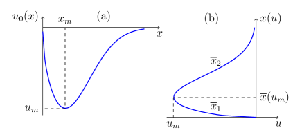
Figure 7: (a) Initial profile of a negative localized pulse. (b) Inverse function is represented by two branches $F_{1}(u)$ and $F_{2}(u)$.

Generalization of this calculation on localized pulses (see Fig. 7) is straightforward and we present here the final results only for $t>t_{m}=t(u_{m})$:

$$\begin{split}t(u)=&\frac{1}{4(-u)^{3/2}}\int_{0}^{u_{m}}\sqrt{-u}\,{{\overline{x}}^{\prime}_{1}(u)}\,du\\ &+\frac{1}{4(-u)^{3/2}}\int_{u_{m}}^{u}\sqrt{-u}\,{{\overline{x}}^{\prime}_{2}(u)}\,du\\ x_{R}(u)=&-\frac{3}{2(-u)^{1/2}}\int_{0}^{u_{m}}\sqrt{-u}\,{{\overline{x}}^{\prime}_{1}(u)}\,du\\ &-\frac{3}{2(-u)^{1/2}}\int_{u_{m}}^{u}\sqrt{-u}\,{{\overline{x}}^{\prime}_{2}(u)}\,du+{\overline{x}}_{2}(u).\end{split}$$ (71)

For asymptotically large time, when $|u|\ll|u_{m}|$ at the soliton edge, we get

$$x_{R}\approx-\frac{3}{2^{1/3}}A^{2/3}t^{1/3},$$ (72)

where

$$A=\int_{0}^{\infty}\sqrt{-u_{0}(x)}\,dx.$$ (73)

The number of waves conservation law (1) can be also reduced to the ordinary differential equation (41) and it should be solved with the boundary condition that $k=0$ at the location of the soliton edge. However, this solution can be found up to the moment $t_{m}$ only when the soliton edge reaches the minimum $u_{m}$ of the smooth solution. At this moment the solution is given by the formula

$$k=2\sqrt{u-u_{m}}$$ (74)

which gives the spectrum of wave numbers generated at the small-amplitude edge. The maximal wave number corresponds to $u=0$ and is given by $k_{m}=2\sqrt{-u_{m}}$. Consequently, the small-amplitude edge propagates at asymptotically large time with the group velocity

$$\frac{dx_{L}}{dt}=\left.\frac{d\omega}{dk}\right|_{k=k_{m}}=12u_{m}.$$ (75)

This estimate is confirmed by numerical simulations.

In the above calculations we did not use the fact of complete integrability of the KdV equation, hence our method can be easily applied to other equations with known harmonic and soliton dispersion laws $\omega(k)$ and $\widetilde{\omega}(\widetilde{k})$.

III.1.3 Generalized KdV equation: Positive pulse

To illustrate the application of our approach to DSWs whose evolution obeys non-integrable wave equations, we shall turn to the generalized KdV equation

$$u_{t}+V(u)u_{x}+u_{xxx}=0,$$ (76)

where we suppose that the function $V(u)$, $V(0)=0$, increases monotonously with growth of $u$ which excludes complications arising in the case of non-genuinely nonlinear situations (see, e.g., kamch-12 ). Other conditions of existence of periodic solutions of this equations and applicability of the Whitham theory of modulations are indicated in Ref. el-05 . The solution of the dispersionless Hopf equation

$$u_{t}+V(u)u_{x}=0$$ (77)

is given in implicit form by the formula

$$x-V(u)t={\overline{x}}(u),$$ (78)

where ${\overline{x}}(u)$ is the function inverse to the initial distribution $u=u_{0}(x)$. [Its non-monotonous version is shown in Fig. 6(b).] We assume that the solution breaks at the moment $t=0$ which imposes the condition $F(u)/V(u)\to 0$ for $|u|\to 0$. The smooth solution matches the small-amplitude edge at $x=x_{L}(t)$ of the DSW and our task now is to find this function $x_{L}(t)$. Proceeding in the same way as in the KdV equation case, we use the number of waves conservation law

$$\frac{\partial k}{\partial t}+\frac{\partial\omega}{\partial x}=0,\qquad\omega(\overline{u},k)=V(\overline{u})k-k^{3}$$ (79)

with $k=k({\overline{u}})$ to reduce it to the differential equation

$$3k\frac{dk}{d{\overline{u}}}=\frac{dV({\overline{u}})}{d{\overline{u}}}$$ (80)

and, extrapolating it on the whole DSW, we solve it with the boundary condition $k(0)=0$ to obtain the wave number $k$ at $x=x_{L}$,

$$k=\sqrt{2V(u)/3}.$$ (81)

Consequently, the velocity of this edge as a function of the value of $u$ at $x=x_{L}$ is given by

$$v_{-}=\frac{d\omega}{dk}=-V(u),$$ (82)

and it corresponds to the characteristic velocity of the limiting Whitham equation

$$\frac{\partial x_{L}}{\partial u}+V(u)\frac{\partial t}{\partial u}=0.$$ (83)

The compatibility condition of this equation with Eq. (78) leads to the differential equation

$$2V(u)\frac{dt}{du}+\frac{dV}{du}\,t=-\frac{d{\overline{x}}}{du}$$ (84)

whose solution with the initial condition $t(0)=0$ reads

$$t(u)=-\frac{1}{2\sqrt{V(u)}}\int_{0}^{u}\frac{{\overline{x}}^{\prime}(u)}{\sqrt{V(u)}}\,du$$ (85)

and, consequently,

$$x(u)=-\frac{\sqrt{V(u)}}{2}\int_{0}^{u}\frac{{\overline{x}}^{\prime}(u)}{\sqrt{V(u)}}\,du+{\overline{x}}(u).$$ (86)

Generalization to localized initial pulses can be done in close analogy with the above considered KdV equation case and it yields the formulas

$$\begin{split}t(u)=&-\frac{1}{2\sqrt{V(u)}}\int_{0}^{u_{m}}\frac{{\overline{x}}^{\prime}_{1}(u)}{\sqrt{V(u)}}\,du\\ &-\frac{1}{2\sqrt{V(u)}}\int_{u_{m}}^{u}\frac{{\overline{x}}^{\prime}_{2}(u)}{\sqrt{V(u)}}\,du\\ x_{L}(u)=&-\frac{\sqrt{V(u)}}{2}\int_{0}^{u_{m}}\frac{{\overline{x}}^{\prime}_{1}(u)}{\sqrt{V(u)}}\,du\\ &-\frac{\sqrt{V(u)}}{2}\int_{u_{m}}^{u}\frac{{\overline{x}}^{\prime}_{2}(u)}{\sqrt{V(u)}}\,du+{\overline{x}}_{2}(u)\end{split}$$ (87)

with obvious notation (see Fig. 6). These formulas define the function $x_{L}(t)$ in parametric form.

Again at the asymptotically large time this pulse evolves into the sequence of solitons whose number can be calculated by the method of Refs. egs-08 ; egkkk-07 . Velocity of the leading soliton can be found with the use of Eq. (4) in vicinity of the moment when the small-amplitude edge reaches the point with $u=u_{m}$. This equation with $\widetilde{k}=\widetilde{k}({\overline{u}})$ reduces to

$$3\widetilde{k}\frac{d\widetilde{k}}{d{\overline{u}}}=-\frac{dV}{d{\overline{u}}}$$ (88)

and it should be solved with the boundary condition $\widetilde{k}=0$ for $u=u_{m}$ which gives

$$\widetilde{k}=\sqrt{2[V(u_{m})-V(u)]/3}.$$ (89)

Since $V(u)$ is a monotonously increasing with $u$ function, we get the maximal value of $\widetilde{k}$, $\widetilde{k}_{m}=\sqrt{2V(u_{m})/3}$, and, consequently, the maximal soliton’s velocity, which is equal to the asymptotic velocity of the soliton edge, is given by the formula

$$\frac{dx_{R}}{dt}=\frac{\omega(\widetilde{k}_{m})}{\widetilde{k}_{m}}=\widetilde{k}_{m}^{2}=\frac{2}{3}V(u_{m}).$$ (90)

III.1.4 Generalized KdV equation: Negative pulse

Now we turn to a situation shown in Fig. 7 with the smooth solution of the dispersionless equation given by

$$x-V(u)t={\overline{x}}(u).$$ (91)

At first we consider a monotonous initial pulse. At the soliton edge the equation

$$\frac{\partial\widetilde{k}}{\partial t}+\frac{\partial\widetilde{\omega}(\widetilde{k})}{\partial x}=0,\quad\widetilde{\omega}({\overline{u}},\widetilde{k})=V({\overline{u}})\widetilde{k}+\widetilde{k}^{3}$$ (92)

can be reduced to the equation

$$3\widetilde{k}\frac{d\widetilde{k}}{d{\overline{u}}}=-\frac{dV}{d{\overline{u}}}$$ (93)

whose extrapolation to the whole DSW followed by solving it with the initial condition $\widetilde{k}(0)=0$ gives

$$\widetilde{k}=\sqrt{-2V(u)/3}.$$ (94)

Hence the soliton edge propagates with velocity

$$v_{+}=\frac{\widetilde{\omega}}{\widetilde{k}}=\frac{1}{3}V(u)$$ (95)

which coincides with the characteristic velocity of the limiting Whitham equation

$$\frac{\partial x_{R}}{\partial u}-\frac{1}{3}V(u)\frac{\partial t}{\partial u}=0.$$ (96)

Its compatibility condition with Eq. (91) leads to the differential equation

$$\frac{2}{3}V(u)\frac{dt}{du}+\frac{dV}{du}=-\frac{d{\overline{x}}}{du}$$ (97)

whose solution with the initial condition $t(0)=0$ yields

$$\begin{split}t(u)=&\frac{3}{2(-V(u))^{3/2}}\int_{0}^{u}{\sqrt{-V(u)}}\,{{\overline{x}}^{\prime}(u)}\,du\\ x_{R}(u)=&-\frac{3}{2\sqrt{-V(u)}}\int_{0}^{u}{\sqrt{-V(u)}}\,{{\overline{x}}^{\prime}(u)}\,du+{\overline{x}}(u).\end{split}$$ (98)

For a localized pulse we obtain the formulas

$$\begin{split}t(u)=&\frac{3}{2(-V(u))^{3/2}}\int_{0}^{u_{m}}{\sqrt{-V(u)}}\,{{\overline{x}}^{\prime}_{1}(u)}\,du\\ &+\frac{3}{2(-V(u))^{3/2}}\int_{u_{m}}^{u}{\sqrt{-V(u)}}\,{{\overline{x}}^{\prime}_{1}(u)}\,du\\ x_{R}(u)=&-\frac{3}{2\sqrt{-V(u)}}\int_{0}^{u_{m}}{\sqrt{-V(u)}}\,{{\overline{x}}^{\prime}_{1}(u)}\,du\\ &-\frac{3}{2\sqrt{-V(u)}}\int_{u_{m}}^{u}{\sqrt{-V(u)}}\,{{\overline{x}}^{\prime}_{1}(u)}\,du+{\overline{x}}_{2}(u)\end{split}$$ (99)

which define in a parametric form the law of motion of the soliton edge. For asymptotically large $t$ we get

$$x_{R}\approx-\left(\frac{3A}{2}\right)^{2/3}t^{1/3},\qquad A=\int_{0}^{\infty}\sqrt{-V(u_{0}(x))}\,dx.$$ (100)

The spectrum of wave numbers generated at the small-amplitude edge can be found by solving the appropriate reduction of Eq. (1) which yields

$$k=\sqrt{2[V(u)-V(u_{m})]/3}$$ (101)

and the small-amplitude edge propagates with the maximal group velocity

$$\frac{dx_{L}}{dt}=\left.\frac{d\omega}{dk}\right|_{k=k_{m}}=2V(u_{m}),$$ (102)

where $k_{m}=\sqrt{-2V(u_{m})/3}$.

The examples considered here demonstrate clearly enough how to apply the method to non-integrable wave equations in the case of unidirectional propagation.

III.2 Bidirectional propagation

We consider here typical situations when the wave is described by the two variables, say, by the density $\rho$ and the flow velocity $u$, and the main supposition is that in the dispersionless limit the equations can be transformed to the Riemann diagonal form

$$\begin{split}&\frac{\partial r_{+}}{\partial t}+v_{+}(r_{+},r_{-})\frac{\partial r_{+}}{\partial x}=0,\\ &\frac{\partial r_{-}}{\partial t}+v_{-}(r_{+},r_{-})\frac{\partial r_{-}}{\partial x}=0\end{split}$$ (103)

for the Riemann invariants $r_{\pm}$. We assume also that at the wave breaking moment one of the Riemann invariants can be considered as constant. In many typical situations, when the initial pulse splits into two well separated pulses corresponding to different characteristic velocities $v_{\pm}$, this assumption is fulfilled by virtue of the wave dynamics and we can consider wave breaking of simple waves only. Besides that, we confine ourselves to situations when this simple wave propagates into uniform quiescent medium so that the arising DSW belongs in integrable cases to the class of quasi-simple waves of Ref. gkm-89 . To compare the results obtained by our method with known formulas derived with the use of the inverse scattering transform method, we shall consider first the integrable NLS equation (21), but we are going to treat it without use of its complete integrability.

III.2.1 NLS equation: Positive profile of $r_{+}$-invariant

We shall start with the situation shown symbolically in Fig. 5(a,b) with the breaking of the invariant $r_{+}=u/2+\sqrt{\rho}$, so that

$$r_{-}=\frac{u}{2}-\sqrt{\rho}=-\sqrt{\rho_{0}},$$ (104)

where $\rho_{0}$ is the density of the quiescent medium into which the pulse propagates. Since $\rho$ and $u$ are related by Eq. (104), it is convenient to consider them as functions of some other variable and, as we shall see, it is convenient for further generalizations to choose the local sound velocity, equal in our present case to $c=\sqrt{\rho}$, as such a variable. Then $u=2(c-c_{0})$, $c_{0}=\sqrt{\rho_{0}}$, $r_{+}=2c-c_{0}$, so that the solution of dispersionless equations can be written as

$$x-(3c-2c_{0})t={\overline{x}}(c-c_{0}),$$ (105)

where ${\overline{x}}(c-c_{0})$ is the function inverse to the initial distribution of the local sound velocity which we shall write in the form $c(x)=c_{0}+\tilde{c}_{0}(x)$, where $\tilde{c}$ denotes a deviation from the background sound velocity $c_{0}$. Thus, we consider the wave breaking in terms of the local sound velocity.

At the boundary with the smooth solution we have now the soliton edge $x_{L}$ of the DSW and the wave breaking diagrams in Fig. 5(a,b) correspond, according to our conjecture, to the applicability conditions of Eq. (4),

$$\frac{\partial\widetilde{k}}{\partial t}+\frac{\partial\widetilde{\omega}(\widetilde{k})}{\partial x}=0,\quad\widetilde{\omega}=\overline{u}\widetilde{k}+\widetilde{k}\sqrt{\overline{\rho}-\widetilde{k}^{2}/4},$$ (106)

where $\overline{\rho},\overline{u}$ are the density and the flow velocity of the background along which solitons propagate. In vicinity of the soliton edge we can consider $\widetilde{k}$ and $\overline{\rho}$ as functions of $c=\sqrt{\overline{\rho}}$ and introduce a new variable

$$\widetilde{\alpha}(c)=\sqrt{1-\frac{\widetilde{k}^{2}(c)}{4c^{2}}},$$ (107)

so that

$$\begin{split}\widetilde{k}(c)&=2c\sqrt{1-\widetilde{\alpha}^{2}},\\ \widetilde{\omega}(c)&=2c\sqrt{1-\widetilde{\alpha}^{2}}[2(c-c_{0})+c\widetilde{\alpha}].\end{split}$$ (108)

With the use of the equation

$$\frac{\partial c}{\partial t}+(u+c)\frac{\partial c}{\partial x}=0,$$ (109)

corresponding to one of the limiting characteristic velocities of the Whitham system and equivalent to Eq. (103) for $r_{+}$, we reduce Eq. (106) to the ordinary differential equation (see the Appendix for more details)

$$\frac{d\widetilde{\alpha}}{dc}=-\frac{1+\widetilde{\alpha}}{c}.$$ (110)

Following El el-05 , we solve it with the boundary condition

$$\widetilde{\alpha}(c_{0})=1$$ (111)

which in our ‘extrapolation’ interpretation means that at the small-amplitude edge the inverse width $\widetilde{k}$ of solitons vanishes together with their amplitude [see Eq. (30)]. As a result, we get

$$\widetilde{\alpha}(c)=\frac{2c_{0}}{c}-1$$ (112)

and

$$V_{s}=\widetilde{\omega}/\widetilde{k}=c.$$ (113)

It corresponds to another limiting characteristic velocity of the Whitham system and the corresponding Whitham equation can be written in the form

$$\frac{\partial x_{L}}{\partial c}-c\frac{\partial t}{\partial c}=0.$$ (114)

The compatibility condition of this equation with Eq. (105) gives with account of Eq. (109)

$$2z\frac{dt}{dz}+3t=-\frac{d{\overline{x}}}{dz},\quad z=c-c_{0}.$$ (115)

Its solution with the initial condition $t(0)=0$ reads

$$t(z)=-\frac{1}{2z^{3/2}}\int_{0}^{z}\sqrt{z}{\overline{x}}^{\prime}(z)dz$$ (116)

and, consequently,

$$x_{L}(z)=(3z+c_{0})t(z)+{\overline{x}}(z).$$ (117)

For example, for the initial profile ${\overline{x}}(z)=-z^{n}$ we get

$$x_{L}(t)=c_{0}t+\frac{n-1}{2n}\left(1+\frac{1}{2n}\right)^{\frac{1}{n-1}}t^{\frac{n}{n-1}}.$$ (118)

This formula coincides, up to the notation, with the result of Ref. kamch-18 obtained from the global solution of the Whitham equations with the use of complete integrability of the NLS equation. Up to the notation, the formulas (116) and (117) reproduce the law of motion of the soliton edge derived in Ref. ekkag-09 in a different physical context of the flow of Bose-Einstein condensate past a wing. All that confirms the validity of our approach.

Generalization of these formulas to the case of localized pulses is straightforward,

$$\begin{split}&t(z)=-\frac{1}{2z^{3/2}}\left\{\int_{0}^{z_{m}}\sqrt{z}{\overline{x}}^{\prime}_{1}(z)dz-\int_{z_{m}}^{z}\sqrt{z}{\overline{x}}^{\prime}_{2}(z)dz\right\},\\ &x_{L}(z)=(3z+c_{0})t(z)+{\overline{x}}_{2}(z).\end{split}$$ (119)

For asymptotically large time we find

$$\begin{split}&x_{L}=c_{0}t+\left(\frac{3A}{2}\right)^{2/3}t^{1/3},\\ &A=\int_{-\infty}^{0}\sqrt{\widetilde{c}_{0}(x)}\,dx,\end{split}$$ (120)

where $c=c_{0}+\widetilde{c}_{0}(x)$ is the initial distribution of the local sound velocity.

To find the velocity of the small-amplitude edge, we have to solve the number of waves conservation law equation

$$\frac{\partial k}{\partial t}+\frac{\partial\omega}{\partial x}=0,\quad\omega=uk+k\sqrt{c^{2}+\frac{k^{2}}{4}}.$$ (121)

Under the same assumptions as above, it can be reduced to the equation (see Appendix)

$$\frac{d\alpha}{dc}=-\frac{1+\alpha}{c}$$ (122)

for the variable

$$\alpha(c)=\sqrt{1+\frac{k^{2}(c)}{4c^{2}}},$$ (123)

so that

$$\begin{split}&k(c)=2c\sqrt{\alpha^{2}-1},\\ &\omega(c)=2c\sqrt{\alpha^{2}-1}[2(c-c_{0})+c\alpha].\end{split}$$ (124)

Now Eq. (122) must be solved with the boundary condition that when the soliton edge reaches the point where $c=c_{m}$, we have $k=0$ and $\alpha(c_{m})=1$. This gives

$$\alpha(c)=\frac{2c_{m}}{c}-1,\quad c_{0}\leq c\leq c_{m},$$ (125)

and $k(c)=4\sqrt{c_{m}(c_{m}-c)}$. Consequently, the range of wave numbers generated at the small-amplitude edge is given by

$$0\leq k\leq k_{m}=4\sqrt{c_{m}(c_{m}-c_{0})},$$ (126)

and it is easy to find that the maximal group velocity is equal to

$$\frac{dx_{R}}{dt}=\left.\frac{d\omega}{dk}\right|_{k=k_{m}}=2r_{m}-\frac{c_{0}^{2}}{r_{m}}$$ (127)

where $r_{m}=2c_{m}-c_{0}$ is the maximum value of $r_{+}$ in its initial distribution. If $c_{0}\ll r_{m}$, then the expression for the velocity of the small-amplitude edge simplifies to

$$\frac{dx_{R}}{dt}\approx 2r_{m}.$$ (128)

Thus, we have found the laws of motion of both edges of the DSW for the case of breaking of the dispersionless invariant $r_{+}$. DSW generated after breaking of the wave propagating in the opposite direction can be considered in a similar way and the resulting formulae differ from the above ones by obvious changes of some signs.

III.2.2 NLS equation: Negative profile of $r_{+}$-invariant

Now we turn to the situation shown symbolically in Figs. 5(c,d) with such breaking of the invariant $r_{+}$ that the smooth solution matches the small-amplitude edge of the DSW and in the integrable approach both Riemann invariants $r_{2}$ and $r_{3}$ change along the DSW. At first we shall find the law of motion of the small amplitude edge.

We represent the smooth solution of the dispersionless equation in the form

$$x-(3c-2c_{0})t={\overline{x}}(c-c_{0}),$$ (129)

where ${\overline{x}}(z)>0$ for $z<0$. Equation (1) can be reduced, as in the preceding section, to Eq. (121) whose solution is looked for with the boundary condition $\alpha(c_{0})=1$ at the soliton edge which gives

$$\alpha(c)=\frac{2c_{0}}{c}-1,\quad 0<c<c_{0},$$ (130)

so that $k=4\sqrt{c_{0}(c_{0}-c)}$. Then the group velocity is equal to

$$v_{-}=\frac{d\omega}{dk}=2c_{0}-\frac{c^{2}}{2c_{0}-c},$$ (131)

and it corresponds to the characteristic velocity of the limiting Whitham equation

$$\frac{\partial x}{\partial c}-\left(2c_{0}-\frac{c^{2}}{2c_{0}-c}\right)\frac{\partial t}{\partial c}=0.$$ (132)

Its compatibility condition with Eq. (129) leads to the differential equation

$$\frac{(4c_{0}-c)(c_{0}-c)}{2c_{0}-c}\frac{dt}{dc}-\frac{3}{2}t=\frac{1}{2}{\overline{x}}^{\prime}(c-c_{0})$$ (133)

whose solution reads

$$\begin{split}&t(c)=\frac{1}{2(4c_{0}-c)\sqrt{c_{0}-c}}\int_{c_{0}}^{c}\frac{(2c_{0}-c){\overline{x}}^{\prime}(c-c_{0})}{\sqrt{c_{0}-c}}dc,\\ &x_{R}(c)=(3c-2c_{0})t(c)+{\overline{x}}(c).\end{split}$$ (134)

In the case of a localized pulse we obtain

$$\begin{split}t(c)=&\frac{1}{2(4c_{0}-c)\sqrt{c_{0}-c}}\Big{\{}\int_{c_{0}}^{c}\frac{(2c_{0}-c){\overline{x}}^{\prime}_{1}(c-c_{0})}{\sqrt{c_{0}-c}}dc\\ &+\int_{c}^{c_{0}}\frac{(2c_{0}-c){\overline{x}}^{\prime}_{2}(c-c_{0})}{\sqrt{c_{0}-c}}dc\Big{\}},\\ x_{R}(c)&=(3c-2c_{0})t(c)+{\overline{x}}_{2}(c).\end{split}$$ (135)

Such a pulse evolves eventually to a sequence of dark solitons and their number can be found with the use of the Bohr-Sommerfeld quantization rule.

For finding the trailing soliton velocity at asymptotically large time we solve Eq. (110) with the boundary condition $\widetilde{k}=0$ at $c=c_{m}$ or $\widetilde{\alpha}(c_{m})=1$. This gives

$$\widetilde{\alpha}(c_{0})=\frac{2c_{m}}{c_{0}}-1,$$ (136)

and consequently the trailing soliton velocity is equal to

$$\frac{dx_{L}}{dt}={\widetilde{\omega}}/{\widetilde{k}}=c_{0}\widetilde{\alpha}(c_{0})=2c_{m}-c_{0}=r_{m}.$$ (137)

We can compare this with the result of the Bohr-Sommerfeld quantization rule (see, e.g., kku-02 ) which gives the expression of the soliton velocity in terms of the Riemann invariants $r_{i},$ $i=1,2,3,4,$ of the Whitham equations, $V_{s}=\tfrac{1}{2}\sum_{i}r_{i}$. In the case of the present initial conditions they are equal to $r_{1}=-\sqrt{\rho_{0}}$, $r_{2}=r_{3}=r_{m}$, $r_{4}=\sqrt{\rho_{0}}$, and we obtain $V_{s}$ coinciding with (137).

III.2.3 Generalized NLS equation: Positive profile of $r_{+}$-invariant

To illustrate application of the method to non-integrable equations, we shall consider the generalized NLS equation

$$i\psi_{t}+\frac{1}{2}\psi_{xx}-f(|\psi|^{2})\psi=0$$ (138)

where the nonlinearity function $f(\rho)$, $f(0)=0$, is supposed to be increasing positive function of the density $\rho=|\psi|^{2}$. Linear harmonic waves propagating along background with density $\rho$ satisfy the dispersion law (121) where

$$c=\sqrt{\rho f^{\prime}(\rho)}$$ (139)

is the sound velocity (see, e.g., ks-09 ). In the dispersionless limit the wave dynamics equations can be written in Riemann form (103) with the Riemann invariants

$$r_{\pm}=\frac{u}{2}\pm\frac{1}{2}\int_{0}^{\rho}\frac{cd\rho}{\rho}$$ (140)

and with the characteristic velocities

$$v_{\pm}=u\pm c.$$ (141)

It is convenient to replace the density $\rho$ as a wave variable by the sound velocity $c$, so that $\rho=\rho(c)$ is the function inverse to $c=c(\rho)$ defined in Eq. (139) and the Riemann invariants take the form

$$r_{\pm}=\frac{u}{2}\pm\sigma(c),\quad\sigma(c)=\frac{1}{2}\int_{0}^{c}\frac{c\rho^{\prime}(c)}{\rho(c)}dc.$$ (142)

Evolution of initial step-like distributions was studied in much detail in Ref. hoefer-14 and we turn here to the problem of evolution of non-uniform initial distributions of simple wave type.

In this section we consider wave breaking of a simple wave with constant Riemann invariant

$$\begin{split}&r_{-}=\frac{u}{2}-\sigma(c)=-\sigma(c_{0}),\\ &\text{i.e.}\quad u=2[\sigma(c)-\sigma(c_{0})].\end{split}$$ (143)

This simple wave propagates into a quiescent medium where the constant sound velocity equals $c_{0}$. Its evolution equation can be written in the form obtained from the first equation (103) with $r_{+}=2\sigma(c)-\sigma(c_{0})$,

$$\frac{\partial c}{\partial t}+(c+u)\frac{\partial c}{\partial x}=0,$$ (144)

whose solution reads

$$x-\left\{2[\sigma(c)-\sigma(c_{0})]+c\right\}t={\overline{x}}(c-c_{0}),$$ (145)

where we suppose that the initial distribution of $c$ is positive, i.e., ${\overline{x}}(c-c_{0})<0$ for $c>c_{0}$ and the inverse function $\widetilde{c}_{0}(x)={\overline{x}}^{-1}(x)$ defines the initial distribution of the local sound velocity $c_{0}+\widetilde{c}_{0}(x)$ such that the wave breaks at the moment $t=0$. The corresponding breaking pattern shown symbolically in Figs. 5(a,b) leads to the formation of DSW with the soliton edge at $x_{L}$. Since in this case Eq. (4) is applicable, we can find the law of motion of this edge by our method.

We write the ‘soliton dispersion law’ in the form (see Eqs. (106) and (107))

$$\widetilde{\omega}=\widetilde{k}(u+c\widetilde{\alpha}(c))$$ (146)

and its substitution together with $\widetilde{k}(c)=2c\sqrt{1-\widetilde{\alpha}^{2}}$ gives with account of Eqs. (143) and (144) the differential equation (see the Appendix)

$$\frac{d\widetilde{\alpha}}{dc}=-\frac{(1+\widetilde{\alpha})(2\sigma^{\prime}(c)+2\widetilde{\alpha}-1)}{c(1+2\widetilde{\alpha})},$$ (147)

which, according to the extrapolation rule, should be solved with the boundary condition $\widetilde{\alpha}(c_{0})=1$, that is the soliton inverse width vanishes together with its amplitude at the small-amplitude edge.

Generally speaking, Eq. (147) can be solved only numerically, but if $\sigma^{\prime}(c)=1/p=\mathrm{const}$, that is

$$f(\rho)=\frac{1}{p}\rho^{p}\quad\text{and}\quad c=\rho^{p/2},$$ (148)

then an easy calculation gives

$$c(\widetilde{\alpha})=c_{0}\left(\frac{2}{1+\widetilde{\alpha}}\right)^{\frac{p}{3p-1}}\left(\frac{2+p}{2-p+2p\widetilde{\alpha}(c)}\right)^{\frac{2(p-1)}{3p-2}}.$$ (149)

Naturally, for $p=1$ this formula reproduces the result (112) of the NLS equation theory. The function $c(\widetilde{\alpha})$ can be also inverted for $p=2$,

$$\widetilde{\alpha}(c)=\frac{1}{2}\left(\sqrt{1+8\left(\frac{c_{0}}{c}\right)^{2}}-1\right),$$ (150)

and for $p=1/2$,

$$\widetilde{\alpha}(c)=\frac{1}{16}\left\{\sqrt{\frac{c_{0}}{c}\left(25\frac{c_{0}}{c}-16\right)}+25\frac{c_{0}}{c}-24\right\}.$$ (151)

Up to the notation, these formulas coincide with those found in Ref. hoefer-14 .

When the function $\widetilde{\alpha}(c)$ is known, we can find the law of motion of the soliton edge. Indeed, the soliton velocity

$$V_{s}=\widetilde{\omega}/\widetilde{k}=2[\sigma(c)-\sigma(c_{0})]+c\widetilde{\alpha}(c)$$ (152)

corresponds to the characteristic velocity of the limiting Whitham equation

$$\frac{\partial x}{\partial c}-\frac{\widetilde{\omega}}{\widetilde{k}}\frac{\partial t}{\partial c}=0,$$ (153)

which must be compatible with Eq. (145) and this condition yields the equation

$$c(1-\widetilde{\alpha}(c))\frac{dt}{dc}+(1+2\sigma^{\prime}(c))t=-{\overline{x}}^{\prime}(c-c_{0}).$$ (154)

Its solution with the initial condition $t(c_{0})=0$ reads

$$\begin{split}t(c)=-G(c)\int_{c_{0}}^{c}\frac{{\overline{x}}^{\prime}(c-c_{0})dc}{c(1-\widetilde{\alpha}(c))G(c)}\end{split}$$ (155)

and, consequently,

$$x_{L}(c)=\left\{2[\sigma(c)-\sigma(c_{0})]+c\right\}t(c)+{\overline{x}}(c-c_{0}),$$ (156)

where

$$G(c)=\exp\left\{-\int_{a}^{c}\frac{(1+2\sigma^{\prime}(c))dc}{c(1-\widetilde{\alpha}(c))}\right\},$$ (157)

the integration limit $a$ is chosen so that the integral is convergent. In fact, the functions $t(c),\,x_{L}(c)$ do not depend on $a$. In particular, for $f(\rho)$ given by Eq. (148) we obtain up to inessential constant factor

$$G(c)=\frac{[1+\widetilde{\alpha}(c)]^{\frac{p+2}{2(3p-2)}}[2p\widetilde{\alpha}(c)+2-p]^{\frac{4(p-1)}{3p-2}}}{[1-\widetilde{\alpha}(c)]^{3/2}}.$$ (158)

Generalization on localized pulses is straightforward and we shall not write down quite lengthy formulas.

As in the case of the standard NLS equation, we can find velocity of the small-amplitude edge at asymptotically large time for a localized initial pulse by solving Eq. (121) provided that the flow velocity $u$ is given by Eq. (143). Then this equation reduces again to Eq. (154), but now it should be solved with the boundary condition

$$\alpha(c_{m})=1,$$ (159)

where $c_{m}$ is the maximal value of the local velocity in the initial distribution $c(x)=c_{0}+\widetilde{c}_{0}(x)$. If $f(\rho)=\rho^{p}/p$, then the solution is given by Eq. (149) or by its particular cases for $p=1,2,1/2$ with $c_{0}$ replaced by $c_{m}$. The spectrum of wave numbers $k=2c\sqrt{\alpha^{2}(c)-1}$ with $c$ in the range $c_{0}\leq c\leq c_{m}$ has the maximal value $k_{m}=2c_{0}\sqrt{\alpha^{2}(c_{0})-1}$ and the corresponding group velocity

$$\frac{dx_{R}}{dt}=\left.\frac{d\omega}{dt}\right|_{k=k_{m}}=2c_{0}\alpha(c_{0})-\frac{c_{0}}{\alpha(c_{0})}$$ (160)

equals the asymptotic velocity of the small-amplitude edge. If $\alpha(c_{0})=2c_{m}/c_{0}-1$, then this formula reproduces the known result (127).

III.2.4 Generalized NLS equation: Negative profile of $r_{+}$-invariant

If the initial profile of local sound velocity $c(x)=c_{0}+\widetilde{c}_{0}(x)$ has the form of a “hole” $\widetilde{c}_{0}(x)<0$, then we represent the smooth dispersionless solution by the formula

$$x-\left\{2[\sigma(c)-\sigma(c_{0})]+c\right\}t={\overline{x}}(c-c_{0}),$$ (161)

where ${\overline{x}}(c-c_{0})>0$ for $c<c_{0}$, that is the initial distribution of $c$ differs from $c_{0}$ at $x>0$ only. Equation (1) reduces again to Eq. (147) and its solution with the boundary condition $\alpha(c_{0})=1$ coincides with Eq. (149) where $\widetilde{\alpha}$ is replaced by $\alpha$ and now we have $\alpha>1$. Correspondingly, in formulas for particular cases $p=1,2,1/2$ (see Eqs. (112), (150), (151)) we should assume $c<c_{0}$.

The small-amplitude edge propagates with the group-velocity

$$\frac{dx_{L}}{dt}=\frac{d\omega}{dk}=2[\sigma(c)-\sigma(c_{0})+c\alpha(c)]-\frac{c}{\alpha(c)},$$ (162)

which can be considered as a characteristic velocity of the limiting Whitham equation

$$\frac{\partial x}{\partial c}-\left\{2[\sigma(c)-\sigma(c_{0})+c\alpha(c)]-\frac{c}{\alpha(c)}\right\}\frac{\partial t}{\partial c}=0.$$ (163)

Its compatibility condition with Eq. (156) leads to the differential equation

$$\frac{c(\alpha(c)-1)(2\alpha(c)+1)}{\alpha(c)}\frac{dt}{dc}-(2\sigma^{\prime}(c)+1)t={\overline{x}}^{\prime}(c-c_{0}),$$ (164)

whose solution with the initial condition $t(c_{0})=0$ reads

$$t(c)=G(c)\int_{c_{0}}^{c}\frac{\alpha(c){\overline{x}}^{\prime}(c-c_{0})dc}{c(\alpha(c)-1)(2\alpha(c)+1)G(c)},$$ (165)

where

$$G(c)=\exp\left\{\int_{a}^{c}\frac{(2\sigma^{\prime}(c)+1)\alpha(c)dc}{c(\alpha(c)-1)(2\alpha(c)+1)}\right\},$$ (166)

which for $f(\rho)$ given by Eq. (148) reduces up to an inessential constant factor to

$$G(c)=\frac{[\alpha(c)+1]^{\frac{p+2}{2(3p-2)}}[2p\alpha(c)+2-p]^{\frac{p-2}{3p-2}}}{\sqrt{\alpha(c)-1}}.$$ (167)

Then we get from Eq. (161)

$$x_{R}(c)=\left\{2[\sigma(c)-\sigma(c_{0})]+c\right\}t(c)+{\overline{x}}(c-c_{0}).$$ (168)

These formulas determine in a parametric form the law of motion of the small-amplitude edge. Their generalization to localized pulses is straightforward.

At asymptotically large time the velocity of the trailing soliton generated from a localized pulse is determined by the value $\widetilde{\alpha}(c_{0})$, where $\widetilde{\alpha}(c)$ is the solution of Eq. (147) with the boundary condition $\widetilde{\alpha}(c_{m})=1$. Then for the velocity of the soliton edge we obtain

$$\frac{dx_{L}}{dt}=c_{0}\widetilde{\alpha}(c_{0})$$ (169)

which generalizes Eq. (137).

IV Comparison with numerical solution

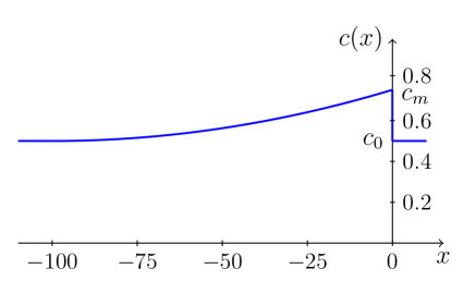
Figure 8: Initial profile of the local sound velocity used in the numerical solution of the generalized NLS equation.

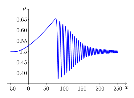
Figure 9: Plot of the density in the DSW evolved from the initial distribution of the local sound velocity $\rho=c(x)$ given by Eq. (170) (for $p=2$ the density is equal to $\rho=c$ and the flow velocity to $u(x)=c(x)-c_{0}$). Evolution time is $t=120$.

To illustrate accuracy of the method, we compare here the results of exact numerical solution of the generalized NLS equation (138) with $f(\rho)$ given by Eq. (148) with $p=2$ for the initial local sound velocity distribution

$$c(x)=0.5+[0.005(x+100)]^{2},\quad-100\leq x\leq 0,$$ (170)

and $c(x)=0.5$ outside this interval; see Fig. 8. A typical form of the DSW generated from such a pulse is shown in Fig. 9. We have chosen the initial distribution with sharp front at $x=0$ to obtain fast enough transition to the asymptotic regime for the small-amplitude edge of the DSW. At the same time, large length of the pulse prevents too fast transition to the asymptotic regime for the soliton edge and therefore the general formulas (155), (156) should be used. In actual numerical solution this sharp transition was slightly smoothed at the front edge, but we neglect here a small contribution of the branch ${\overline{x}}_{1}(c-c_{0})$ of the inverse function $x={\overline{x}}(c-c_{0})$ and take into account only the branch

$${\overline{x}}(c-c_{0})={\overline{x}}_{2}(c-c_{0})=200\sqrt{c-c_{0}}-100.$$ (171)

In our case with $p=2$ we have $\sigma(c)=c/2$, $\widetilde{\alpha}(c)$ is given by Eq. (150), so an elementary integration in the formula (157) yields

$$G(c)=\frac{c+\sqrt{c^{2}+8c_{0}^{2}}}{[(c+\sqrt{c^{2}+8c_{0}^{2}})^{2}-16c_{0}^{2}]^{3/2}},$$ (172)

where we have omitted an inessential constant factor which cancels in the formulas

$$\begin{split}&t(c)=-2G(c)\int_{c_{m}}^{c}\frac{{\overline{x}}^{\prime}(c-c_{0})dc}{\left(3c-\sqrt{{c}^{2}+8c_{0}^{2}}\right)G(c)},\\ &x_{L}(c)=(2c-c_{0})t(c)+{\overline{x}}(c-c_{0}).\end{split}$$ (173)

Substitution of Eq. (171) gives the parametrical dependence $x=x_{L}(t)$ shown in Fig. 10 by a dashed line. As we can see, it agrees reasonably well without any fitting parameter with the result of numerical solution shown by a solid line.

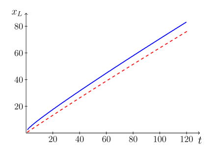
Figure 10: Law of motion of the soliton edge. Solid (blue) line shows the result of numerical solution and dashed (red) line corresponds to the analytical formulas (173).

For finding the law of motion of the small-amplitude edge, we use the formula (160) with

$$\alpha(c_{0})=\frac{1}{2}\left(\sqrt{1+8\left(\frac{c_{m}}{c_{0}}\right)^{2}}-1\right),$$ (174)

which gives the velocity $dx_{R}/dt\approx 1.356$ (we take $c_{m}=0.742$, $c_{0}=0.5$ which corresponds to the actual initial distribution). A linear dependence with this slope fits well to the numerical solution shown in Fig. 11. This agreement should be considered as very good since the position of the small-amplitude edge is not very certain, as is clear from Fig. 9, and we determine it by means of an approximate extrapolation of the envelopes of the wave at this edge. Some irregularities in the numerical plot in Fig. 11 correspond to changes of the amplitude maxima and minima used in such an extrapolation at different moments of time.

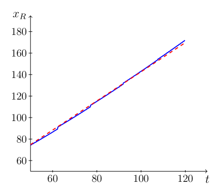
Figure 11: Linear law of motion of the small-amplitude edge with the slope calculated according to Eq. (160) (red dashed line) and from the numerical solution (blue solid line).

The above comparison of the analytical predictions with the numerical solution demonstrates quite convincingly that the method suggested here gives accurate enough description of pulses whose evolution obeys non-integrable equations.

V Conclusion

We have shown that Whitham’s number of waves conservation law (1) and its soliton counterpart (4) allow one to calculate the main parameters of DSWs for a wide class of initial conditions including the pulses propagating into a medium ‘at rest’. Here we formulate the main principles of this method.

(i) While Eq. (1) is universally correct in framework of the Whitham theory, Eq. (4) has limited applicability and we have presented argumentation in favor of its applicability to situations when the pulse under consideration propagates into a medium at rest at some reference frame.

(ii) For a given initial distribution of the simple-wave type, the smooth solution of the dispersionless equations can be considered as known and at its boundary with DSW Eqs. (1) and (4) reduce to ordinary differential equations which can be extrapolated to the whole DSW, and then their solution with known boundary condition at the opposite edge yields the wave number $k$ or the inverse half-width of solitons $\widetilde{k}$ at the boundary with the smooth part of the pulse. This procedure is equivalent to El’s approach el-05 .

(iii) Consequently, the corresponding group velocity or the soliton’s velocity at the DSW edge can be expressed in terms of the parameters of the smooth solution at its boundary with DSW.

(iv) These velocities can be treated as the characteristic velocities of the limiting Whitham equations at this edge and this can be represented as the hodograph transformed form of the first order partial differential equation.

(v) At last, the compatibility condition of this partial differential equation with the smooth dispersionless solution yields the law of motion of this edge of DSW. If the soliton solution is known, then the soliton’s amplitude related with its velocity can be also found.

This scheme reproduces the known results when it is applied to the completely integrable equations, and its applicability to non-integrable equations is confirmed by comparison with the results of numerical simulations. Thus, the method suggested here permits one to calculate parameters of DSWs in a number of interesting physical problems. The results obtained here can be applied to various nonlinear optics models that reduce to different forms of generalized NLS equation (see, e.g., kivshar-08 ). Applications to shallow water waves described by different nonlinear wave models (see, e.g. the review kdfm-18 ) or to DSWs in nonlinear lattices (see, e.g., kst-97 ) and in systems described by the Gardner equation (see, e.g., sp-99 ) are also of great interest.

Appendix A. Equations for $\alpha(c)$ and $\widetilde{\alpha}(c)$

Here we give for completeness some details of derivation of equations for $\alpha(c)$ and $\widetilde{\alpha}(c)$ directly from Eqs. (1) and (4). Since in both cases the calculations are very similar, we shall consider the equation for the small-amplitude edge of DSW where the Whitham number of waves conservation law

$$\frac{\partial k}{\partial t}+\frac{\partial\omega}{\partial x}=0$$ (A.1)

holds. We write the dispersion law in the form

$$\omega(c,k)=uk+ck\alpha(c,k),\quad\alpha(c,k)=\sqrt{1+\frac{k^{2}}{4c^{2}}},$$ (A.2)

where the first term in the right-hand side represents the Doppler shift of the frequency caused by the flow of the medium with velocity $u$ and the factor $\alpha(c,k)$ describes deviation of the dispersion law from the dispersionless limit $\omega=ck$, $k\to 0$ $(u=0)$, $c$ being the local sound velocity.

In dispersionless limit the generalized NLS equation (138) takes a hydrodynamic form which can be cast into equations for the Riemann invariants (142). We consider the DSW evolving from a simple wave with constant $r_{-}=\mathrm{const}$ which gives according to the Gurevich-Meshcherkin conjecture gm-84 the expression for $u$ in terms of $c$,

$$u=2[\sigma(c)-\sigma(c_{0})].$$ (A.3)

Consequently, $r_{+}=2\sigma(c)-\sigma(c_{0})$ is a function of $c$ only and the equation for $r_{+}$ reduces to the equation for $c$,

$$\frac{\partial c}{\partial t}+(u+c)\frac{\partial c}{\partial x}=0.$$ (A.4)

Following El el-05 , we assume that $k$ is also a function of $c$, so substitution of (A.2) and (A.3) into (A.1) with account of (A.4) yields after obvious cancellations the equation

$$\frac{1}{k}\frac{dk}{dc}\,c(1-\alpha)=2\sigma^{\prime}+\alpha+c\alpha^{\prime}.$$ (A.5)

From definition of $\alpha$ in Eq. (A.2) we get

$$k(c)=2c\sqrt{\alpha^{2}(c)-1}$$ (A.6)

and substitution of this expression into Eq. (A.5) yields equation for $\alpha(c)$,

$$\frac{d\alpha}{dc}=-\frac{(\alpha+1)(2\sigma^{\prime}+2\alpha-1)}{c(2\alpha+1)}.$$ (A.7)

The equation for $\widetilde{\alpha}(c)$ can be obtained in a similar way.

It is worth noticing that many other physical systems differ from the case considered here by the linear dispersion law only, that is by the concrete form of the expression for $\alpha(c,k)$. If this expression is solved with respect to $k$, then substitution of $k=k(c,\alpha(c))$ into Eq. (A.5) gives the equation for $\alpha(c)$ for the system under consideration.

References

- (1) L. D. Landau and E. M. Lifshitz, Fluid Mechanics (Pergamon, Oxford, 1987).
- (2) R. Courant, K. O. Friedrichs, Supersonic Flow and Shock Waves, Interscience Publishers, New York (1948).
- (3) T. B. Benjamin, M. J. Lighthill, Proc. Roy. Soc. London, A 224, 448 (1954).
- (4) R. Z. Sagdeev, Rev. Plasma Phys., 4, 23 (1966).
- (5) R. S. Johnson, J. Fluid Mech., 42, 49 (1970).
- (6) A. V. Gurevich, L. P. Pitaevskii, Sov. Phys. JETP, 38, 291 (1974).
- (7) G. B. Whitham, Proc. Roy. Soc. London, A 283, 238 (1965).
- (8) G. B. Whitham, Linear and Nonlinear Waves, Wiley, N. Y., 1974.
- (9) G. A. El, M. A. Hoefer, Physica D, 333, 11 (2016).
- (10) H. Flaschka, M. G. Forest, and D. W. McLaughlin, Commun. Pure Appl. Math., 33, 379 (1980).
- (11) C. S. Gardner, J. M. Green, M. D. Kruskal, and R. M. Miura, Phys. Rev. Lett., 19, 1095 (1967).
- (12) P. D. Lax, Comm. Pure Appl. Math., 28, 141 (1974).
- (13) S. P. Novikov, Funct. Anal. Appl., 8, 236 (1974).
- (14) I. M. Krichever, Funct. Anal. Appl., 22, 200 (1988).
- (15) S. P. Tsarev, Math. USSR Izvestia, 37, 397 (1991).
- (16) B. A. Dubrovin, S. P. Novikov, Sov. Sci. Rev. C. Math. Phys., 9, 1 (1993).
- (17) M. G. Forest, D. W. McLaughlin, SIAM J. Appl. Math., 44, 287 (1984).
- (18) V. V. Avilov, I. M. Krichever, S. P. Novikov, Sov. Phys. Dokl., 32, 564 (1987).
- (19) A. V. Gurevich, L. P. Pitaevskii, Sov. Phys. JETP, 66, 490 (1988).
- (20) S. Myint, R. Grimshaw, Wave Motion, 22, 215 (1995).
- (21) A. M. Kamchatnov, Physica D, 188, 247 (2004).
- (22) A. V. Gurevich, A. P. Meshcherkin, Sov. Phys. JETP, 60, 732 (1984).
- (23) G. A. El, Chaos, 15, 037103 (2005).
- (24) O. Akimoto and K. Ikeda, J. Phys. A: Math. Gen., 10, 425 (1977); K. Ikeda and O. Akimoto, J. Phys. A: Math. Gen. 12, 1105 (1979).
- (25) S. A. Darmanyan, A. M. Kamchatnov, M. Neviére, JETP, 96, 876–884 (2003).
- (26) G. A. El, R. H. J. Grimshaw, N. F. Smyth, Phys. Fluids, 18, 027104 (2006).
- (27) G. A. El, A. Gammal, E. G. Khamis, R. A. Kraenkel, A. M. Kamchatnov, Phys. Rev. A, 76, 053813 (2007).
- (28) G. A. El, R. H. J. Grimshaw, N. F. Smyth, J. Fluid Mech., 640, 187 (2009).
- (29) J. G. Esler, J. D. Pearce, J. Fluid Mech., 667, 555 (2011).
- (30) M. A. Hoefer, J. Nonlinear Sci., 24, 525 (2014).
- (31) T. Congy, A. M. Kamchatnov, and N. Pavloff, SciPost Phys., 1, 006 (2016).
- (32) M. A. Hoefer, G. A. El, A. M. Kamchatnov, SIAM J. Appl. Math., 77, 1352 (2017).
- (33) X. An, T. R. Marchant, N. F. Smyth, Proc. Roy. Soc. London A, 474, 20180278 (2018).
- (34) G. A. El, R. H. J. Grimshaw, N. F. Smyth, Physica D, 237, 2423 (2008).
- (35) A. V. Gurevich, A. L. Krylov, N. G. Mazur, Sov. Phys. JETP, 68, 966 (1989).
- (36) A. M. Kamchatnov, Zh. Eksp. Teor. Fiz. 154, 1016 (2018) [JETP, 127, 903 (2018)].
- (37) J. L. Hammack and H. Segur, J. Fluid Mech., 65, 289 (1974); ibid., J. Fluid Mech., 84, 337 (1978).
- (38) S. Trillo, M. Klein, G. F. Clauss, M. Onorato, Physica D, 333, 276 (2016).
- (39) W. Wan, S. Jia, and J. W. Fleischer, Nature Phys., 3, 46 (2007).
- (40) J. Fatome, C. Finot, G. Millot, A. Armaroli, and S. Trillo, Phys. Rev. X, 4, 021022 (2014)
- (41) G. Xu, M. Conforti, A. Kudlinski, A. Mussot, S. Trillo, Phys. Rev. Lett., 118, 254101 (2017)
- (42) M. A. Hoefer, M. J. Ablowitz, I. Coddington, E. A. Cornell, P. Engels, and V. Schweikhard, Phys. Rev. A, 74, 023623 (2006).
- (43) P. Engels, C. Atherton, Phys. Rev. Lett., 99, 160405 (2007).
- (44) J. J. Chang, P. Engels, and M. A. Hoefer, Phys. Rev. Lett., 101, 170404 (2008).
- (45) A. M. Kamchatnov, Nonlinear Periodic Waves and Their Modulations. An Introductory Course, World Scientific, Singapore, 2000.
- (46) V. I. Karpman, Phys. Lett. A, 26, 619 (1968).
- (47) M. G. Forest and J. E. Lee, “Geometry and modulation theory for periodic nonlinear Schrodinger equation”, in Oscillation Theory, Computation, and Methods of Compensated Compactness, Eds. C. Dafermos et al, IMA Volumes on Mathematics and its Applications 2, Springer, N.Y., 1986.
- (48) M. V. Pavlov, Theor. Math. Phys., 71, 351 (1987).
- (49) A. M. Kamchatnov, R. A. Kraenkel, and B. A. Umarov, Phys. Rev. E, 66, 036609 (2002).
- (50) V. R. Kudashev, S. E. Sharapov, Theor. Math. Phys., 85, 205 (1990).
- (51) A. V. Gurevich, A. L. Krylov, N. G. Mazur, and G. A. El, Sov. Phys. Dokl., 37, 198 (1992).
- (52) V. R. Kudashev, JETP Lett. 56, 320 (1992).
- (53) A. M. Kamchatnov, arXiv:1810.04844.
- (54) A. M. Kamchatnov, Y.-H. Kuo, T.-C. Lin, T.-L. Horng, S.-C. Gou, R. Clift, G. A. El, and R. H. J. Grimshaw, Phys. Rev. E, 86, 036605 (2012).
- (55) G. A. El, A. M. Kamchatnov, V. V. Khodorovskii, E. S. Annibale, and A. Gammal, Phys. Rev. E, 80, 046317 (2009).
- (56) A. M. Kamchatnov and M. Salerno, J. Phys. B: At. Mol. Opt. Phys., 42, 185303 (2009).
- (57) Yu. S. Kivshar, Spatial Optical Solitons, in Nonlinear Science at the Dawn of the 21st Century, Eds. P.L. Christiansen, M.P. Sorensen, A.C. Scott, Springer, Berlin, 2008.
- (58) G. Khakimzyanov, D. Dutykh, Z. Fedotova, and D. Mitsotakis, Commun. Comput. Phys., 23, 1, (2018).
- (59) V. V. Konotop, M. Salerno,, and S. Takeno, Phys. Rev. E, 56, 7240 (1997).
- (60) A. V. Slyunyaev, E. N. Pelinovsky, JETP, 89, 173 (1999).