Generalized Low-Rank Optimization for Topological Cooperation in Ultra-Dense Networks

Abstract

Network densification is a natural way to support dense mobile applications under stringent requirements, such as ultra-low latency, ultra-high data rate, and massive connecting devices. Severe interference in ultra-dense networks poses a key bottleneck. Sharing channel state information (CSI) and messages across transmitters can potentially alleviate interferences and improve system performance. Most existing works on interference coordination require significant CSI signaling overhead and are impractical in ultra-dense networks. This paper investigate topological cooperation to manage interferences in message sharing based only on network connectivity information. In particular, we propose a generalized low-rank optimization approach to maximize achievable degrees-of-freedom (DoFs). To tackle the challenges of poor structure and non-convex rank function, we develop Riemannian optimization algorithms to solve a sequence of complex fixed rank subproblems through a rank growth strategy. By exploiting the non-compact Stiefel manifold formed by the set of complex full column rank matrices, we develop Riemannian optimization algorithms to solve the complex fixed-rank optimization problem by applying the semidefinite lifting technique and Burer-Monteiro factorization approach. Numerical results demonstrate the computational efficiency and higher DoFs achieved by the proposed algorithms.

I Introduction

The upsurge of wireless applications, including Internet-of-Things (IoT), Tactile Internet, tele-medicine and mobile edge artificial intelligence, is driving the paradigm shift of wireless networks from content delivery to skillset-delivery networks [1]. Network densification [2] has emerged as a promising approach to support innovative mobile applications with stringent requirements such as ultra-low latency, ultra-high data rate and massive devices connectivity. Unfortunately, interference in dense wireless network deployment becomes a key capacity limiting factor given large numbers of transmitters and receivers. Network cooperation through sharing channel state information (CSI) and messages among transmitting nodes is a viable technology to improve the spectral efficiency and energy efficiency in ultra-dense wireless networks.

Under shared CSI among transmitters, interference alignment [3] is shown to mitigate interferences base on linear coding schemes, capable of achieving half the cake for each user in $K$-user interference channel. Cooperative transmission [4] with message sharing has shown to be able to further improve system throughput. In particular, through centralized signal processing and interference management with full message sharing via the cloud data center, cloud radio access network (Cloud-RAN) [5] can harness the advantages of network densification. By pushing the storage resources to the network edge [6], cache-aided wireless network [7] provides a cost effective way to enable transmission cooperation.

Unfortunately, most existing works on network cooperation lead to significant channel signaling overhead. This is practically challenging in ultra-dense networks. A growing body of recent works has hence been focusing on CSI acquisition overhead reduction for interference coordination in wireless networks. Among them, delay effect in CSI acquisition has been considered in [8]. Both [9] and [10] have studied transceiver design using partial CSI, requiring instantaneous CSI for strong links and only distribution CSI of the remaining weak links. In addition, finite precision CSI feedback [11] and the compressed channel estimation [12] can further reduce CSI acquisition overhead.

However, the applicability of the aforementioned results in practical systems remains unclear, which motivates a recent proposal on topological interference management (TIM) [13]. The main idea of TIM is to manage the interference based only on the network connectivity information, which can significantly reduce the CSI acquisition overhead. By requiring only network topologies, TIM becomes one of the most promising and powerful schemes for interference management in ultra-dense wireless networks. By further enabling message sharing, the work of [14] shows that transmitter cooperation based only on network topology information can strictly improve the degrees-of-freedom (DoFs). However, their results are only applicable to some specific network connectivity patterns.

In this paper, we propose a generalized low-rank optimization approach for investigating the benefits of topological cooperation for any network topology. We begin by first establishing the generalized interference alignment conditions based only on the network connectivity information with message sharing among transmitters. A low-rank model is further developed to maximize the achievable DoFs by exploiting the relationship between the model matrix rank and the achievable DoFs. The developed low-rank matrix optimization model thus generalizes the low-rank matrix completion model [15] without message sharing among transmitters. Unfortunately, the resulting generalized low-rank optimization problem in complex field is non-convex and highly intractable due to poor structure, for which novel and efficient algorithms need to be developed.

Low-rank matrix optimization models have wide range of applications in machine learning, high-dimensional statistics, signal processing and wireless networks [15, 16, 17, 18]. A wealth of recent works focus on both convex approximation and non-convex algorithms to solve the non-convex and highly intractable low-rank optimization problems. Nuclear norm is a well-known convex proxy for non-convex rank function with optimality guarantees under statistical models [19]. To further reduce the storage and computation overhead for low-rank optimization, non-convex approach based on matrix factorization shows good promises [20]. With suitable statistical models, the non-convex methods can also find globally optimal solution for some structured optimization problems such as matrix completion [21]. In particular, the work of [22] adopted an alternating minimization algorithm to exploit topological transmitter cooperation gains. This algorithm stores the iterative results in the factored form and optimizes over one factor while fixing the other.

Nevertheless, the nuclear norm based convex relaxation approach in fact fails to solve the formulation of generalized low-rank matrix optimization problem because of the poor structures. Actually, the nuclear norm minimization approach always yields a full-rank matrix solution. Alternating minimization [20] algorithm by factorizing the fixed-rank matrix is particularly useful when the resulting problem is biconvex with respect to the two factors in matrix factorization. However, the convergence of the alternating minimization algorithm heavily depends on the initial points with slow convergence rates. It may also yield poor performance in achievable DoFs, as it only guarantees convergence to the first-order stationary points [15, 22]. In contrast, Riemannian optimization [23] approach has shown to be effective in improving the achievable DoFs by solving the low-rank matrix optimization problems, as the Riemannian trust-region algorithm guarantees convergence to the second-order stationary points with high precision solutions [15]. Furthermore, the Riemannian optimization algorithms are robust to initial points in ensuring convergence [24] with fast convergence rates. However, no available Riemannian optimization algorithms have been developed for the general non-square low-rank problems in the complex field. In this work, we develop Riemannian optimization algorithms for solving the presented generalized low-rank optimization problem in the complex field.

I-A Contributions

In this paper, we develop a generalized interference alignment condition to enable transmitter cooperation based only on the network topology information. We present a generalized low-rank model to maximize the achievable DoFs. To address the special challenges in the resulting generalized low-rank optimization problem, we develop Riemannian optimization algorithms by exploiting the non-compact Stiefel manifold of fixed-rank matrices in complex field. Specifically, we propose to solve the generalized low-rank optimization problem by solving a sequence of fixed rank subproblems with rank increase. By applying semidefinite lifting technique [25], the fixed rank subproblem is reformulated as a positive semidefinite matrix problem in complex field with rank constraint. By applying the Burer-Monteiro [26] parameterization approach to factorize the positive semidefinite matrix, the resulting problem turns out to be a Riemannian optimization problem on complex non-compact Stiefel manifold. Therefore, the generalized low-rank optimization problem can be successfully solved by developing Riemannian optimization algorithms on the complex-valued non-compact Stiefel manifold.

We summarize the main contributions of this work as follows:

1. We establish a generalized interference alignment condition to enable transmitter cooperation with message sharing based only on network connectivity information. We develop a generalized low-rank model to maximize the achievable DoFs.

2. We develop first-order and second-order Riemannian optimization algorithms for solving the generalized low-rank optimization problem in complex field. We exploit the complex compact Stiefel manifold of complex fixed-rank matrices using the semidefinite lifting and Burer-Monteiro factorization techniques.

3. Numerical results demonstrate that the proposed second-order Riemannian trust-region algorithm is able to achieve the highest DoFs with high precision second-order stationary point solutions. Furthermore, its computing time is comparable to the first-order Riemannian conjugate gradient algorithm in medium network sizes. Overall, the Riemannian algorithms show much better performance than the alternating minimization algorithm.

I-B Organization and Notation

The remainder of this paper is organized as follows. In Section II, we first introduce the system model, before establishing the generalized topological interference alignment conditions. We develop the generalized low-rank model in Section III, and derive a positive semidefinite reformulation with the Burer-Monteiro approach to address the low-rank optimization problem in complex field. We derive Riemannian algorithms on complex non-compact Stiefel manifold in Section IV. Section V provides simulation results. Finally, we conclude this work in Section VI,

We use $[K]$ denote the set $\{1,2,\cdots,K\}$. $\mathbb{S}_{+}^{N}$ denotes the set of all $N\times N$ Hermitian positive semidefinite matrices. And $\langle\cdot,\cdot\rangle$ denotes inner product, i.e., $\langle{\bm{A}},{\bm{X}}\rangle={\textrm{Tr}}({\bm{A}}^{\sf{H}}{\bm{X}})$.

II System Model and Problem Formulation

In this section, we establish the generalized interference alignment condition for partially connected $K$-user interference channel with transmitter cooperation.

II-A System Model

Consider a partially-connected interference channel with $K$ single-antenna transmitters and $K$ single-antenna receivers. Transmitters aim to deliver a set of independent messages $W_{1},W_{2}$, $\cdots,W_{K}$ to receivers $1,\,2,\,\cdots,\,K$, respectively. Transmitter $k$ has message $W_{k}$ and is always connected with receiver $k$. The channel coefficient $h_{kl}\in\mathbb{C}$ between the $l$-th transmitter and the $k$-th user is nonzero only for $(k,l)\in\mathcal{E}$. Block fading channel model is considered in this paper, i.e., $h_{kl}$ remains stationary in $r$ consecutive channel uses, during which the input-output relationship is given by

$${\bm{y}}_{k}=\sum_{(k,i)\in\mathcal{E}}{h}_{ki}{{\bm{x}}}_{i}+{\bm{z}}_{k},~{}\forall k\in[K],$$ (1)

where ${{\bm{x}}}_{i}\in\mathbb{C}^{r}$ is the transmitted signal at transmitter $i$, ${\bm{y}}_{k}\in\mathbb{C}^{r}$ is the received signal at receiver $k$, and ${\bm{z}}_{k}\in\mathbb{C}^{r}$ is the additive isotropic white Gaussian noise, i.e., ${\bm{z}}_{k}\sim\mathcal{CN}({\bm{0}},{\bm{\Sigma}}_{k})$ with ${\bm{\Sigma}}_{k}\in\mathbb{C}^{r\times r}$. Partial connectivity of the interference channel provides opportunities to enable cooperative transmission based only on the network connectivity information. Specifically, transmitter cooperation is enabled with message sharing, for which we denote the index set of messages available at transmitter $k$ as $\mathcal{S}_{k}\subseteq[K]$. A $5$-user example of such system is shown in Fig. 1.

Let $R(W_{k})$ be the achievable data rate of message $W_{k}$, i.e., there exists a coding scheme such that the rate of message $W_{k}$ is $R(W_{k})$ and the decoding error probability can be arbitrarily small. Let SNR denote the signal-to-noise-ratio. For each message delivery, the degree-of-freedom (DoF) [13], the first order characterization of channel capacity, is defined as

$$\textrm{DoF}(W_{k})=\lim_{\textrm{SNR}\rightarrow\infty}\frac{R(W_{k})}{\log(\textrm{SNR})},~{}\forall k\in[K].$$ (2)

The set of achievable DoF allocation is denoted as $\{\textrm{DoF}(W_{1}),\cdots,\textrm{DoF}(W_{K})\}$, whose closure is called the DoF region. This paper adopts DoF as the performance metric and designs a linear coding scheme.

II-B Linear Coding Strategy

Linear coding scheme is attractive for interference management owing to its low complexity. Specifically, its optimality in terms of DoF has been shown via interference alignment [3]. Its effectiveness has been demonstrated in the problems of topological interference management (TIM) and index coding [13]. We thus focus on linear coding scheme to design low complexity and efficient approaches for maximizing achievable DoFs.

Suppose each message $W_{k}$ is represented by a complex vector ${\bm{s}}_{k}\in\mathbb{C}^{d_{k}}$ with $d_{k}$ data streams. Let ${{\bm{V}}}_{kj}\in\mathbb{C}^{r\times d_{j}}$ be the precoding matrix at transmitter $k$ for message $W_{j}$. Then the transmitted signal is given by

$${\bm{x}}_{k}=\sum_{j\in\mathcal{S}_{k}}{\bm{V}}_{kj}{\bm{s}}_{j}.$$ (3)

Consequently, the received signal at user $k$ is

$${\bm{y}}_{k}=\!\!\!\!\!\!\!\!\!\!\!\!\sum_{j:(k,j)\in\mathcal{E},k\in\mathcal{S}_{j}}\!\!\!\!\!\!\!\!\!\!h_{kj}{\bm{V}}_{jk}{\bm{s}}_{k}+\sum_{i\neq k}\sum_{j:(k,j)\in\mathcal{E},i\in\mathcal{S}_{j}}\!\!\!\!\!\!\!h_{kj}{\bm{V}}_{ji}{\bm{s}}_{i}+{\bm{z}}_{k}.$$ (4)

We let ${\bm{U}}_{k}\in\mathbb{C}^{r\times d_{k}}$ be the decoding matrix at receiver $k$.

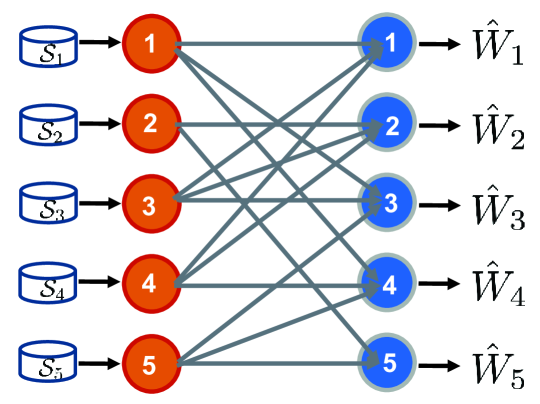
Figure 1: The architecture of the partially-connected $K$-user interference channel with transmitter cooperation. $\mathcal{S}_{i}$ denotes the index set of messages available at transmitter $i$.

In densified wireless networks, interference is a key bottleneck to support high data rate and low latency. To alleviate interferences by aligning the intersection of interference spaces, the following interference alignment conditions were presented in [13, 27]

$$\sum\limits_{j:(k,j)\in\mathcal{E},k\in\mathcal{S}_{j}}h_{kj}{\bm{U}}_{k}^{\sf{H}}{\bm{V}}_{jk} \neq 0,~{}\forall k\in[K],$$ (5)

$$\sum\limits_{j:(k,j)\in\mathcal{E},i\in\mathcal{S}_{j}}h_{kj}{\bm{U}}_{k}^{\sf{H}}{\bm{V}}_{ji} = 0,~{}i\neq k.$$ (6)

Correspondingly, the message at receiver $k$ is decoded via

$$\hat{{\bm{s}}}_{k}=(\!\!\!\!\!\!\sum\limits_{j:(k,j)\in\mathcal{E},k\in\mathcal{S}_{j}}\!\!\!\!\!\!h_{kj}{\bm{U}}_{k}^{\sf{H}}{\bm{V}}_{jk})^{-1}{\bm{U}}_{k}^{\sf{H}}{\bm{y}}_{k}.$$ (7)

If there exists ${\bm{U}}_{k}$’s, ${\bm{V}}_{ji}$’s satisfying interference alignment conditions (5) and (6), DoF tuple $({d_{1}}{r}^{-1},\cdots,{d_{K}}{r}^{-1})$ is then achievable. We thus can achieve the highest DoF by finding the minimal channel use number $r$.

II-C Topology-Based Alignment Condition

Note that equations (5) and (6) are always feasible by increasing $r$. However, the interference alignment conditions (5) and (6) require the knowledge of channel coefficients $h_{ij}$s at the transmitters. In practice, obtaining dense network channel state information (CSI) at transmitters often requires large signaling overhead, which presents a severe obstacle to their application in densified wireless networks. One desirable way to address the CSI acquisition overhead issue is to establish new interference alignment conditions based only on the network connectivity information, for which we present the following generalized interference alignment conditions for topological cooperation

$$\textrm{det}\left(\sum_{j:(k,j)\in\mathcal{E},k\in\mathcal{S}_{j}}{{\bm{U}}}_{k}^{\sf{H}}{{\bm{V}}}_{jk}\right)\neq 0,~{}~{}\forall k\in[K],$$ (8)

$${\bm{U}}_{k}^{\sf{H}}{\bm{V}}_{ji}={\bm{0}},~{}~{}i\in\mathcal{S}_{j},i\neq k,(k,j)\in\mathcal{E}.$$ (9)

Here, “topological cooperation” refers to the fact that for cooperation enabled transmitters, we design transceivers to manage interferences based on network topology information instead of instantaneous channel state information.

Proposition 1.

For generic channel coefficients $h_{ij}$’s randomly distributed according to some continuous probability distribution [28], if (8) and (9) hold for some ${\bm{U}}_{k},{\bm{V}}_{ji}$s based only on the network topology information, then they shall satisfy the channel dependent interference alignment conditions (5) and (6) with probability 1.

Proof.

Let ${\bm{Z}}_{1},\cdots,{\bm{Z}}_{T}\in\mathbb{C}^{d\times d}$ denote the set of matrices $\{{\bm{U}}_{k}^{\sf{H}}{\bm{V}}_{jk}:(k,j)\in\mathcal{E},k\in\mathcal{S}_{j}\}$ given $k$. Our goal is to prove that if $\textrm{det}\Big{(}\sum_{t=1}^{T}{\bm{Z}}_{t}\Big{)}\neq 0$, the probability of $\textrm{det}\Big{(}\sum_{t=1}^{T}h_{t}{\bm{Z}}_{t}\Big{)}\neq 0$ is $1$ for generic $h_{1},\cdots,h_{T}$. Note that $\sum_{t=1}^{T}{\bm{Z}}_{t}=\begin{bmatrix}{\bm{Z}}_{1}&\cdots&{\bm{Z}}_{T}\end{bmatrix}\begin{bmatrix}{\bm{I}}&\cdots&{\bm{I}}\end{bmatrix}^{H}$. Thus, the condition $\textrm{det}\Big{(}\sum_{t=1}^{T}{\bm{Z}}_{t}\Big{)}\neq 0$ implies that $\begin{bmatrix}{\bm{Z}}_{1}&\cdots&{\bm{Z}}_{T}\end{bmatrix}$ has full rank, i.e., the dimension of $\textrm{span}\{{\bm{Z}}_{j}\}$ is $r$. Since the solution to the determinant equation $\textrm{det}\Big{(}\sum_{t=1}^{T}h_{t}{\bm{Z}}_{t}\Big{)}=0$ is an algebraic hypersurface [27], the probability of the linear combination $\sum_{t=1}^{T}h_{t}{\bm{Z}}_{t}$ with generic coefficients $h_{1},\cdots,h_{T}$ lying on the algebraic hypersurface is hence zero. Therefore, $\textrm{det}\Big{(}\sum_{t=1}^{T}h_{t}{\bm{Z}}_{t}\Big{)}\neq 0$ holds with probability $1$. ∎

By leveraging conditions (8) and (9), interferences can be aligned based only on network topology CSI instead of full CSI. This significantly reduces the overhead of CSI acquisition. In particular, the topological interference alignment condition without message sharing is given by [15]

$$\textrm{det}\left({{\bm{U}}}_{k}^{\sf{H}}{{\bm{V}}}_{k}\right)\neq 0,~{}~{}\forall k\in[K],$$ (10)

$${\bm{U}}_{k}^{\sf{H}}{\bm{V}}_{j}={\bm{0}},~{}~{}j\neq k,(k,j)\in\mathcal{E},$$ (11)

which is a special case of (8) and (9) with $\mathcal{S}_{j}=\{j\}$ and ${{\bm{V}}}_{j}$ denoting as ${{\bm{V}}}_{jj}$. Conditions (8) and (9) thus manifest the benefits of transmitter cooperation, as solutions to (10) and (11) are always solutions to (8) and (9), but not conversely.

Remark 1.

This work assumes that there are equal number of transmitters and receivers. Nevertheless, the principle applies for arbitrary number of transmitters and receivers. This is because both Proposition 1 and the low-rank matrix representation for precoding and decoding matrices in Section 3 hold for any number of transmitters and receivers. For simplicity of notation we consider a system with $K$ transmitters and receivers in this paper.

III Generalized Low-Rank Optimization for Topological Cooperation

This section develops a generalized low-rank optimization framework to maximize achievable DoFs under topological cooperation. To address the challenges of the present generalized low-rank optimization problem in complex field and to exploit the algorithmic benefits of Riemannian optimization, we propose to reformulate an optimization problem over the complex non-compact Stiefel manifold by using the semidefinite lifting and Burer-Monteiro approaches.

III-A Generalized Low-Rank Model for Topological Cooperation

Without loss of generality, we restrict $\sum_{j:(k,j)\in\mathcal{E},k\in\mathcal{S}_{j}}{{\bm{U}}}_{k}^{\sf{H}}{{\bm{V}}}_{jk}={\bm{I}}$ in condition (8). By letting $m=\sum_{k}d_{k},~{}n=K\sum_{k}d_{k}$ and defining

$${\bm{U}} =\begin{bmatrix}{\bm{U}}_{1}&\cdots&{\bm{U}}_{K}\end{bmatrix}\in\mathbb{C}^{r\times m},$$

$${\bm{V}}_{j} =[{{\bm{V}}}_{j1},\cdots,{{\bm{V}}}_{jK}]\in\mathbb{C}^{r\times m},$$

$${\bm{V}} =\begin{bmatrix}{\bm{V}}_{1}&\cdots&{\bm{V}}_{K}\end{bmatrix}\in\mathbb{C}^{r\times n},$$

$${\bm{X}} =[{\bm{X}}_{kj}^{i}]=[{\bm{U}}_{k}^{\sf{H}}{\bm{V}}_{ji}]={{\bm{U}}}^{\sf{H}}{{\bm{V}}}\in\mathbb{C}^{m\times n},$$

the rank of matrix ${\bm{X}}$ is given as

$$\textrm{rank}(\bm{X})=r=d_{k}/\text{DoF}(W_{k}).$$ (12)

We thus can maximize the achievable DoF for interference-free message delivery by solving the following generalized low-rank optimization problem

$$\mathscr{P}:\mathop{\textrm{minimize}}_{{{\bm{X}}}\in\mathbb{C}^{m\times n}} \textrm{rank}({{\bm{X}}})$$

subject to $$\mathcal{A}({{\bm{X}}})={{\bm{b}}},$$ (13)

where the affine constraint $\mathcal{A}({{\bm{X}}})={{\bm{b}}}$ captures

$$\sum_{j:(k,j)\in\mathcal{E},k\in\mathcal{S}_{j}}{\bm{X}}_{kj}^{k}={\bm{I}},~{}\forall k\in[K]$$ (14)

$${\bm{X}}_{kj}^{i}={\bm{0}},~{}i\neq k,i\in\mathcal{S}_{j},(k,j)\in\mathcal{E}$$ (15)

and $\mathcal{A}:\mathbb{C}^{m\times n}\mapsto\mathbb{C}^{l}$.

For the simpler case without message sharing, the topological interference alignment problem can be formulated as the following low-rank matrix completion problem [15, 29]

$$\mathop{\textrm{minimize}}_{\bm{X}\in\mathbb{C}^{m\times m}} \textrm{rank}({\bm{X}})$$

subject to $${\bm{X}}_{kk}={\bm{I}},~{}\forall k\in[K]$$ (16)

$${\bm{X}}_{kj}={\bm{0}},~{}j\neq k,(k,j)\in\mathcal{E},$$

which is a special case of problem $\mathscr{P}$. The resulting low-rank matrix completion model is demonstrated in Fig. 2.

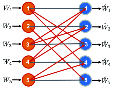
(a) TIM

(b) Matrix Completion Model

Figure 2: Matrix completion model for the topological interference alignment without message sharing for single data stream $d_{k}=1$. In this case, all the diagonal entries are set to 1 as $\mathcal{S}_{k}=\{k\}$. As an example, the $(2,3)$-th entry is zero because the second receiver is connected with the third transmitter as interference. And the $(3,2)$-th entry of the matrix can be arbitrary value as $(3,2)\not\in\mathcal{E}$.

III-B Problem Analysis

Basically, methods for solving low-rank problems can be divided into two categories. One uses convex relaxation approach and the other one uses nonconvex approach based on matrix factorization. In addition, penalty decomposition method is proposed in [30] for low-rank optimization problems. The inner iterations adopt a block coordinated descent method, whereas the outer iterations update the weight of rank function. However, each inner iteration requires the computation of singular value decomposition, which leads to large computation overhead ($\mathcal{O}(mnl+m^{2}n+m^{3})$). Therefore, it is not suitable for our tranceiver design problem in ultra-dense networks.

III-B1 Convex Relaxation Methods

Nuclear norm is a well-known convex proxy [16] for rank function. The nuclear norm relaxation approach for problem $\mathscr{P}$ is given by

$$\mathop{\textrm{minimize}}_{{{\bm{X}}}\in\mathbb{C}^{m\times n}} \|{{\bm{X}}}\|_{*}$$

subject to $$\mathcal{A}({{\bm{X}}})={{\bm{b}}}.$$ (17)

It can be solved by an equivalent semidefinite programming (SDP) problem

$$\mathop{\textrm{minimize}}_{{\bm{X}},{\bm{W}}_{1},{\bm{W}}_{2}} \textrm{Tr}({\bm{W}}_{1})+\textrm{Tr}({\bm{W}}_{2})$$

subject to $$\mathcal{A}({{\bm{X}}})={{\bm{b}}},$$

$$\begin{bmatrix}{\bm{W}}_{1}&{\bm{X}}\\ {\bm{X}}^{\sf{H}}&{\bm{W}}_{2}\end{bmatrix}\succeq{\bm{0}}.$$

Unfortunately, the SDP solution requires computing singular value decomposition at each iteration, which is not scalable to large problem sizes in ultra-dense networks. Specifically, with high precision second-order interior point method, the convergence rate is fast while the computational cost for each iteration is $\mathcal{O}((mn+l)^{3})$ due to computing the Newton step [31]. Using the first-order algorithm alternating direction method of multipliers (ADMM) [32], the computational cost is $\mathcal{O}(mnl+m^{2}n+m^{3})$ at each iteration. Furthermore, the nuclear norm relaxation approach always yields a full rank solution due to the poor structure of the affine operator $\mathcal{A}$.

Proposition 2.

The nuclear norm relaxation approach (III-B1) for the generalized low-rank optimization problem $\mathscr{P}$ always yields a full rank solution.

Proof.

See Appendix A. ∎

Therefore, the nuclear norm relaxation based approach is inapplicable for the poorly structured low-rank optimization problem $\mathscr{P}$. We thus call problem $\mathscr{P}$ as the generalized low-rank optimization problem.

III-B2 Nonconvex Approaches

A rank $r$ matrix ${{\bm{X}}}$ can be factorized as ${{\bm{X}}}={{\bm{L}}}{{\bm{R}}}^{\sf{H}}$, where ${{\bm{L}}}\in\mathbb{C}^{m\times r}$ and ${{\bm{R}}}\in\mathbb{C}^{n\times r}$. Nonconvex approaches to low-rank optimization leverage matrix factorizations and design various updating strategies for two factors $\bm{U}$ and $\bm{V}$. By solving a sequence of the fixed rank least square subproblems based on matrix factorization

$$\mathop{\textrm{minimize}}_{{{\bm{X}}}\in\mathbb{C}^{m\times n}} f_{0}({{\bm{X}}})=\frac{1}{2}\|\mathcal{A}({{\bm{X}}})-{{\bm{b}}}\|_{2}^{2}$$

subject to $$\textrm{rank}({{\bm{X}}})=r,$$ (19)

and increasing $r$, we can find the minimal rank $r$ for the original problem $\mathscr{P}$.

Specifically, for the rank constrained problem (III-B2) with convex objective function, the alternating minimization [20] algorithm can function as follows:

$$\bm{L}_{k+1} = \arg\min_{{{\bm{L}}}}~{}~{}f_{0}({\bm{L}}{\bm{R}}_{k}^{\sf{H}}),$$ (20)

$$\bm{R}_{k+1} = \arg\min_{{{\bm{R}}}}~{}~{}f_{0}({\bm{L}}_{k+1}{\bm{R}}^{\sf{H}}).$$ (21)

It essentially optimizes the bi-convex objective function $f_{0}(\bm{L}\bm{R}^{\sf{H}})$ by freezing one of ${{\bm{L}}}$ and ${{\bm{R}}}$ alternatively. However, the convergence of the alternating minimization algorithm are sensitive to initial points and its convergence rate can be slow. Furthermore, it may yield poor performance for achievable DoFs maximization by only converging to first-order stationary point.

In contrast, Riemannian optimization algorithms are capable of updating the two factors $\bm{L}$ and $\bm{R}$ simultaneously by exploiting the quotient manifold geometry of fixed-rank matrices based on matrix factorization. First-order Riemannian conjugate gradient and second-order Riemannian trust-region algorithm can help find first-order stationary points and second-order stationary points, respectively. It has been shown in [24] that Riemannian optimization algorithms converge to first-order and second-order stationary points from arbitrary initial points. Furthermore, Riemannian trust-region algorithm can achieve high achievable DoFs with second-order stationary points while also enjoys locally super-linear [23] convergence rates.

Remark 2.

The invariance of matrix factorization $({\bm{L}}{\bm{M}}^{\sf{H}},{\bm{M}}^{-1}{\bm{R}})$ for any full rank matrix ${\bm{M}}$ makes the critical points of $f_{0}$ parameterized with ${\bm{L}}$ and ${\bm{R}}$ are not isolated in Euclidean space. This indeterminancy profoundly affects the convergence of second-order optimization algorithms [33, 34]. To address this issue, we shall develop efficient algorithms on the quotient manifold instead of Euclidean space.

Unfortunately, available Riemannian algorithms for non-square fixed-rank matrix optimization problems only operate in $\mathbb{R}$ field [23] and do not directly apply to solve problem (III-B2) in the complex filed. Inspired by the fact that the complex non-compact Stiefel manifold is well defined [35], we propose to reformulate complex matrix optimization problem (III-B2) on the complex non-compact Stiefel manifold by using the Burer-Monteiro approach. Specifically, applying semidefinite lifting, the original problem (III-B2) is equivalently reformulated into rank constrained positive semidefinite matrix optimization, before factorizing the semidefinite matrices using the Burer-Monteiro approach. The original complex matrix optimization problem (III-B2) is thus reformulated as the Riemannian optimization problem over the well-defined non-compact Stiefel manifold in complex field.

III-C Semidefinite Lifting and the Burer-Monteiro Approach

Burer-Monteiro approach is a well-known nonconvex parameterization method for solving positive semidefinite (PSD) matrices problems [26]. A rank $r$ PSD matrix ${{\bm{Z}}}\in\mathbb{S}^{N}$ can be factorized as ${{\bm{Z}}}={{\bm{Y}}}{{\bm{Y}}}^{\sf{H}}$ with ${{\bm{Y}}}\in\mathbb{C}^{N\times r}$. The linear operator $\mathcal{A}$ can be represented as a set of matrices ${\bm{A}}_{i}\in\mathbb{C}^{n\times m}$, i.e.,

$$\mathcal{A}({{\bm{X}}})=[\langle{\bm{A}}_{i},{\bm{X}}\rangle],i=1,\cdots,l.$$ (22)

Then the objective function in (III-B2) can be rewritten as

$$f_{0}({\bm{X}})=\frac{1}{2}\sum_{i=1}^{l}|\langle{\bm{A}}_{i},{\bm{X}}\rangle-b_{i}|^{2}.$$ (23)

By semidefinite lifting [25] ${{\bm{X}}}$ to

$${{\bm{Z}}}=\begin{bmatrix}{{\bm{Z}}}_{11}&{{\bm{Z}}}_{12}\\ {{\bm{Z}}}_{21}&{{\bm{Z}}}_{22}\end{bmatrix}:=\begin{bmatrix}{{\bm{L}}}{{\bm{L}}}^{\sf{H}}&{{\bm{L}}}{{\bm{R}}}^{\sf{H}}\\ {{\bm{R}}}{{\bm{L}}}^{\sf{H}}&{{\bm{R}}}{{\bm{R}}}^{\sf{H}}\end{bmatrix},$$ (24)

we can reformulate problem (III-B2) as a complex PSD matrix problem with rank constraint:

$$\mathop{\textrm{minimize}}_{{{\bm{Z}}}\in\mathbb{S}_{+}^{N}} \frac{1}{2}\|\mathcal{B}({{\bm{Z}}})-{{\bm{b}}}\|_{2}^{2}$$

subject to $$\textrm{rank}({{\bm{Z}}})=r,$$ (25)

where $N=m+n$ and

$$\mathcal{B}({\bm{Z}})=\mathcal{A}({\bm{Z}}_{12})=\mathcal{A}({{\bm{L}}}{{\bm{R}}}^{\sf{H}}).$$ (26)

Here we use $\mathcal{B}$ to denote a set of matrices ${\bm{B}}_{i}\in\mathbb{C}^{N\times N}$

$${\bm{B}}_{i}=\begin{bmatrix}{\bm{0}}&{\bm{A}}_{i}\\ {\bm{0}}&{\bm{0}}\end{bmatrix},\langle{\bm{B}}_{i},{\bm{Z}}\rangle=\langle{\bm{A}}_{i},{\bm{X}}\rangle.$$ (27)

We define ${{\bm{Y}}}=\begin{bmatrix}{{\bm{L}}}\\ {{\bm{R}}}\end{bmatrix}\in\mathbb{C}^{N\times r}$. The search space $\{\bm{Z}:\bm{Z}\in\mathbb{S}_{+}^{N},\textrm{rank}({{\bm{Z}}})=r\}$ admits a well-defined manifold structure, by factorizing $\bm{Z}=\bm{Y}\bm{Y}^{\sf{H}}$ based on the principles of Burer-Monteiro approach. Problem (III-C) thus can be transformed as

$$\mathop{\textrm{minimize}}_{{{\bm{Y}}}\in\mathbb{C}_{*}^{N\times r}} f({{\bm{Y}}})=\frac{1}{2}\|\mathcal{B}({\bm{Y}}{\bm{Y}}^{\sf{H}})-{\bm{b}}\|_{2}^{2}.$$ (28)

This is a Riemannian optimization problem with a smooth ($C^{\infty}$) objective function over the complex non-compact Stiefel manifold $\mathbb{C}_{*}^{N\times r}$, i.e., the set of all $N\times r$ full column rank matrices in complex field.

In summary, we propose to solve the generalized low-rank optimization problem by solving a sequence of complex fixed-rank optimization problem using the Riemannian optimization technique. This is achieved by lifting the complex fixed-rank optimization problem into the complex positive semidefinite matrix optimization problem, followed by parameterizing it using the Burer-Monteior approach. This yields the Riemannian optimization problem over complex non-compact Stiefel manifold. After obtaining a solution ${\bm{Y}}$ from (28), we can recover the solution ${\bm{X}}={{\bm{L}}}{{\bm{R}}}^{\sf{H}}$ to the original problem (III-B2). The whole algorithm of addressing the transmitter cooperation problem based only on the network topology information is demonstrated in Algorithm 1.

Input: $\{S_{j}\},\mathcal{E},K,\{d_{k}\}$, accuracy $\varepsilon$.

Construct $\mathcal{B}$ and $\bm{b}$ following (14) (15) (22) (27). Let $N=m+n=(K+1)\sum_{k}d_{k}$.

for $r=1,\cdots,N$ do

       Solve (28) with Riemannian optimization algorithm.

       if $f({{\bm{Y}}}^{[r]})<\varepsilon$ then

            return ${\bm{Y}}^{[r]}$

       end if

      

end for

Output: $\bm{Y}^{[r]}$ and rank $r$.

Algorithm 1 Optimization Framework for Transmitter Cooperation Based on Network Topology Information

IV Matrix Optimization on Complex Non-compact Stiefel Manifold

In this section, we shall develop Riemannian conjugate gradient and Riemannian trust-region algorithms for solving problem (28). Riemannian optimization generalizes the concepts of gradient and Hessian in Euclidean space to Riemannian gradient and Hessian on manifolds. They are represented in the tangent space, which is the linearization of the search space.

IV-A Quotient Geometry of Fixed-Rank Problem

For problem (28), the optima are not isolated because of ${{\bm{Y}}}{{\bm{Y}}}^{\sf{H}}$ remains invariant under the canonical projection [23, Sec 3.4.1]

$$\pi:~{}{{\bm{Y}}}\mapsto{{\bm{Y}}}{{\bm{Q}}}$$ (29)

for any unitary matrix ${{\bm{Q}}}\in\mathcal{U}(r)$ where $\mathcal{U}(r)$ denotes the set of $r\times r$ unitary matrices. To address this non-uniqueness we consider problem (28) over the equivalent class

$$[{{\bm{Y}}}]=\{{{\bm{Y}}}{{\bm{Q}}}:{{\bm{Y}}}\in\overline{\mathcal{M}}=\mathbb{C}_{*}^{N\times r},{{\bm{Q}}}\in\mathcal{U}(r)\},$$ (30)

that is

$$\mathop{\textrm{minimize}}_{[{{\bm{Y}}}]\in\mathcal{M}} f([{{\bm{Y}}}]).$$ (31)

Then the whole set of feasible solutions can be represented by isolated points in the quotient manifold, i.e. $\mathcal{M}=\overline{\mathcal{M}}/\sim:=\overline{\mathcal{M}}/\mathcal{U}(r)$ with canonical projection [23, Sec 3.4] $\pi$. Here $\sim$ is the equivalence relation and $\overline{\mathcal{M}}/\sim:=\{[{\bm{Y}}]:{\bm{Y}}\in\overline{\mathcal{M}}\}$. $\overline{\mathcal{M}}$ is considered as an abstract manifold.

IV-B Riemannian Ingredients for Iterative Algorithms on Riemannian Manifolds

By studying the unconstrained problem on the quotient manifold instead of the constrained problem in Euclidean space, Riemannian optimization can exploit the non-uniqueness of matrix factorization with Burer-Monteiro approach. We now develop conjugate gradient and trust-region algorithms on the Riemannian manifold. To achieve this goal, we first linearize the search space, by defining the concept of tangent space [23, Sec 3.5] and associated “inner product” on the tangent space. Next, we will derive the expressions for Riemannian gradient and Riemannian Hessian in this subsection.

Specifically, tangent space $\mathcal{T}_{{\bm{Y}}}\overline{\mathcal{M}}$ is a vector space consisting of all tangent vectors to $\overline{\mathcal{M}}$ at ${\bm{Y}}$.

Proposition 3.

The tangent space of $\overline{\mathcal{M}}=\mathbb{C}_{*}^{N\times r}$ at ${\bm{Y}}$ is given by $\mathcal{T}_{{\bm{Y}}}\overline{\mathcal{M}}=\mathbb{C}^{N\times r}$.

Proof.

$\overline{\mathcal{M}}$ is an open submanifold [23, Sec 3.5.2] of $\mathbb{C}^{N\times r}$ and hence, $\mathcal{T}_{{\bm{Y}}}\overline{\mathcal{M}}=\mathbb{C}^{N\times r}$ for all ${\bm{Y}}\in\overline{\mathcal{M}}$. ∎

In order to eliminate the non-uniqueness along the equivalent class $[{\bm{Y}}]$, we will decompose the tangent space into two orthogonal parts, i.e., vertical space and horizontal space. Vertical space $\mathcal{V}_{{\bm{Y}}}$ is the tangent space of equivalent class $[{\bm{Y}}]$, while horizontal space $\mathcal{H}_{{\bm{Y}}}$ is the orthogonal complement of vertical space in the tangent space. That is,

$$\mathcal{T}_{{\bm{Y}}}\overline{\mathcal{M}}=\mathcal{V}_{{\bm{Y}}}\oplus\mathcal{H}_{{\bm{Y}}},$$ (32)

where $\oplus$ denotes the direct sum of two subspace. In this way, we can always find the unique “lifted” representation of the tangent vectors of $\mathcal{T}_{[{\bm{Y}}]}\mathcal{M}$ in $\mathcal{T}_{{\bm{Y}}}\overline{\mathcal{M}}$ at any element of $[{\bm{Y}}]$, i.e., for any ${\bm{\xi}}\in\mathcal{T}_{{\bm{Y}}}\mathcal{M}$ we define a unique horizontal lift $\overline{{\bm{\xi}}}\in\mathcal{H}_{{\bm{Y}}}$ at ${\bm{Y}}$ such that

$$\overline{{\bm{\xi}}}:=\Pi_{{\bm{Y}}}^{h}{\bm{\xi}},$$ (33)

where horizontal projection $\Pi_{{\bm{Y}}}^{h}(\cdot)$ is the orthogonal projection from $\mathcal{T}_{{\bm{Y}}}\mathcal{M}$ onto $\mathcal{H}_{{\bm{Y}}}$.

Proposition 4.

The vertical space at ${\bm{Y}}$ is given by

$$\mathcal{V}_{{\bm{Y}}}\triangleq\{{\bm{Y}}{\bm{\Omega}}:{\bm{\Omega}}^{\sf{H}}=-{\bm{\Omega}},{\bm{\Omega}}\in\mathbb{C}^{r\times r}\}.$$ (34)

Proof.

See Appendix B. ∎

According to the definition, horizontal space should be derived from

$$\mathcal{H}_{{\bm{Y}}}=\{\overline{{\bm{\xi}}}\in\mathcal{T}_{{\bm{Y}}}\overline{\mathcal{M}}:\overline{g}_{{\bm{Y}}}(\overline{{\bm{\xi}}},\overline{{\bm{\zeta}}})=0,~{}\forall\overline{{\bm{\zeta}}}\in\mathcal{V}_{{\bm{Y}}}\},$$ (35)

where $\overline{g}$ is Riemannian metric for the abstract manifold $\overline{\mathcal{M}}$. Riemannian metric is the generalization of “inner product” in Euclidean space to a manifold. It is a bilinear, symmetric positive-definite operator

$$\overline{g}:~{}\mathcal{T}_{{\bm{Y}}}\overline{\mathcal{M}}\times\mathcal{T}_{{\bm{Y}}}\overline{\mathcal{M}}\mapsto\mathbb{R}.$$ (36)

In this paper, we can choose

$$\overline{g}_{{\bm{Y}}}(\overline{{\bm{\xi}}},\overline{{\bm{\zeta}}}):={\textrm{Tr}}(\Re(\overline{{\bm{\xi}}}^{\sf{H}}\overline{{\bm{\zeta}}}))=\frac{1}{2}\textrm{Tr}(\overline{{\bm{\xi}}}^{\sf{H}}\overline{{\bm{\zeta}}}+\overline{{\bm{\zeta}}}^{\sf{H}}\overline{{\bm{\xi}}})$$ (37)

as a Riemannian metric for the abstract manifold $\overline{\mathcal{M}}$, where ${\bm{Y}}\in\overline{\mathcal{M}}$ and $\overline{{\bm{\xi}}},\overline{{\bm{\zeta}}}\in\mathcal{T}_{{\bm{Y}}}\overline{\mathcal{M}}$. The manifold $\overline{\mathcal{M}}$ is called a Riemannian manifold when its tangent spaces are endowed with a Riemannian metric. From another perspective, $\overline{\mathcal{M}}$ can also be viewed as a Kähler manifold whose Kähler form is a real closed (1,1)-form [36].

Therefore, we can obtain the explicit expressions for the horizontal space and horizontal projection.

Proposition 5.

The horizontal space is

$$\mathcal{H}_{{\bm{Y}}}=\{{\bm{\xi}}\in\mathbb{C}^{N\times r}:{\bm{\xi}}^{\sf{H}}{\bm{Y}}={\bm{Y}}^{\sf{H}}{\bm{\xi}}\},$$ (38)

and the orthogonal projection onto the horizontal space is

$$\Pi_{{\bm{Y}}}^{h}{\bm{\xi}}_{{\bm{Y}}}={\bm{\xi}}_{{\bm{Y}}}-{\bm{Y}}{\bm{\Omega}},$$ (39)

where ${\bm{\Omega}}^{\sf{H}}=-{\bm{\Omega}}\in\mathbb{C}^{r\times r}$ is the solution of Lyapunov equation

$${\bm{Y}}^{\sf{H}}{\bm{Y}}{\bm{\Omega}}+{\bm{\Omega}}{\bm{Y}}^{\sf{H}}{\bm{Y}}={\bm{Y}}^{\sf{H}}{\bm{\xi}}_{{\bm{Y}}}-{\bm{\xi}}_{{\bm{Y}}}^{\sf{H}}{\bm{Y}}.$$ (40)

Proof.

See Appendix C. ∎

Given the Riemannian metric for the abstract manifold, quotient manifold is naturally endowed with a Riemannian metric

$$g_{[{\bm{Y}}]}({\bm{\xi}}_{[{\bm{Y}}]},{\bm{\zeta}}_{[{\bm{Y}}]}):=\overline{g}_{{\bm{Y}}}(\overline{{\bm{\xi}}}_{{\bm{Y}}},\overline{{\bm{\zeta}}}_{{\bm{Y}}})$$ (41)

such that the expression $\overline{g}_{{\bm{Y}}}(\overline{{\bm{\xi}}}_{{\bm{Y}}},\overline{{\bm{\zeta}}}_{{\bm{Y}}})$ remains for any elements in the equivalent class $[{\bm{Y}}]$. Hence $\mathcal{M}$ is a Riemannian quotient manifold of the abstract manifold $\overline{\mathcal{M}}$ with the Riemannian metric $g$, and the canonical projection $\pi:(\overline{\mathcal{M}},\overline{g})\mapsto(\mathcal{M},g)$ is a Riemannian submersion [23, Sec 3.6.2].

Riemannian optimization generalizes the gradient and Hessian into Riemannian gradient and Riemannian Hessian.

$\mathop{\textrm{minimize}}_{[{{\bm{Y}}}]\in\overline{\mathcal{M}}}~{}f({{\bm{Y}}})$
Computation space	$\overline{\mathcal{M}}=C_{*}^{N\times r},\mathcal{M}=\overline{\mathcal{M}}/\sim$
Canonical projection	$\pi:{\bm{Y}}\mapsto{\bm{Y}}{\bm{Q}},{{\bm{Q}}}\in\mathcal{U}(r)\qquad$	(29)
Remannian metric	$g_{{\bm{Y}}}({\bm{\xi}}_{{\bm{Y}}},{\bm{\eta}}_{{\bm{Y}}})=\textrm{Tr}({\bm{\xi}}_{{\bm{Y}}}^{\sf{H}}{\bm{\eta}}_{{\bm{Y}}}+{\bm{\eta}}_{{\bm{Y}}}^{\sf{H}}{\bm{\xi}}_{{\bm{Y}}})\qquad$	(37)
Vertical space	$\mathcal{V}_{{\bm{Y}}}=\{{\bm{Y}}{\bm{\Omega}}:{\bm{\Omega}}^{\sf{H}}=-{\bm{\Omega}},{\bm{\Omega}}\in\mathbb{C}^{r\times r}\}\qquad$	(34)
Horizontal space	$\mathcal{H}_{{\bm{Y}}}=\{{\bm{\xi}}\in\mathbb{C}^{N\times r}:{\bm{\xi}}^{\sf{H}}{\bm{Y}}={\bm{Y}}^{\sf{H}}{\bm{\xi}}\}\qquad$	(38)
Projection onto horizontal space	$\Pi_{\mathcal{M}}^{h}{\bm{\xi}}_{{\bm{Y}}}={\bm{\xi}}_{{\bm{Y}}}-{\bm{Y}}{\bm{\Omega}}\qquad$	(39)
Remannian gradient	$\textrm{grad}f({\bm{Y}})=\sum_{i=1}^{l}(C_{i}{\bm{B}}_{i}+C_{i}^{*}{\bm{B}}_{i}^{\sf{H}}){\bm{Y}}\qquad$	(44)
Remannian Hessian	$\textrm{Hess}f({\bm{Y}})[{\bm{\eta}}_{{\bm{Y}}}]\qquad$	(IV-B2)
Retraction	$\mathcal{R}_{{\bm{Y}}}({\bm{\xi}})=\pi({\bm{Y}}+\overline{{\bm{\xi}}})\qquad$	(49)

TABLE I: Riemannian ingredients

IV-B1 Riemannian Gradient

Riemannian gradient is a necessary ingredient to develop the Riemannian conjugate gradient and Riemannian trust-region algorithm. For quotient manifold, the horizontal representation of Riemannian gradient, denoted by $\textrm{grad}f({\bm{Y}})$, arises from

$$\textrm{grad}f({\bm{Y}})=\Pi_{{\bm{Y}}}^{h}\overline{\textrm{grad}}f({\bm{Y}}),$$ (42)

in which $\overline{\textrm{grad}}f({\bm{Y}})$ is the Riemannian gradient in the abstract manifold $\overline{\mathcal{M}}$ at ${\bm{Y}}$. Note that $\overline{\textrm{grad}}f({\bm{Y}})$ is given by

$$\overline{g}_{{\bm{Y}}}(\overline{\textrm{grad}}f({\bm{Y}}),\overline{{\bm{\xi}}})=\textrm{D}f({\bm{Y}})[\overline{{\bm{\xi}}}],~{}\forall\overline{{\bm{\xi}}}\in\mathcal{T}_{{\bm{Y}}}\overline{\mathcal{M}},$$ (43)

where $\textrm{D}f({\bm{Y}})[{\bm{\xi}}]:=\lim_{t\rightarrow 0}t^{-1}\left[f({\bm{Y}}+t{\bm{\xi}})-f({\bm{Y}})\right]$ is the directional derivative of $f$, whereas $\overline{{\bm{\xi}}}$ is the horizontal lift of ${\bm{\xi}}$. Then we conclude that

$$\textrm{grad}f({\bm{Y}})=\overline{\textrm{grad}}f({\bm{Y}})=\sum_{i=1}^{l}(C_{i}{\bm{B}}_{i}+C_{i}^{*}{\bm{B}}_{i}^{\sf{H}}){\bm{Y}},$$ (44)

in which $C_{i}=\langle{\bm{B}}_{i},{\bm{Y}}{\bm{Y}}^{\sf{H}}\rangle-b_{i}$. The derivation process is described in detail in Appendix D.

IV-B2 Riemannian Hessian

For the purpose of developing a second-order algorithm, we need to think of the Riemannian Hessian as an linear operator closely connected to the directional derivative of the gradient. Riemannian connection defines a “directional derivative” on the Riemannian manifold. To be specific, Euclidean directional derivative is a Riemannian connection on $\mathbb{C}^{N\times r}$. Since the quotient manifold $\mathcal{M}$ has a Riemannian metric that is invariant along the horizontal space, the Riemannian connection [23, Proposition 5.3.4] can be derived from

$$\nabla_{\bm{\eta}}\bm{\xi}=\Pi_{\bm{Y}}^{h}(\textrm{D}\overline{\bm{\xi}}[\overline{\bm{\eta}}]),$$ (45)

for any $\bm{\eta}\in\mathcal{V}_{{\bm{Y}}},\;\bm{\xi}\in\mathfrak{X}(\mathcal{M})$ and $\mathfrak{X}(\mathcal{M})$ is the set of smooth vector fields on $\mathcal{M}$. The horizontal representation of Riemannian Hessian operator [23, Definition 5.5.1] is given as

$$\textrm{Hess}f({\bm{Y}})[{\bm{\xi}}_{{\bm{Y}}}]:=\nabla_{{\bm{\xi}}_{{\bm{Y}}}}\overline{\textrm{grad}}f.$$ (46)

Then the Riemannian Hessian is given by

$$\textrm{Hess}f({\bm{Y}})[{\bm{\eta}}_{{\bm{Y}}}]=\Pi_{{\bm{Y}}}^{h}\biggl{(} \sum_{i=1}^{l}({C_{{\bm{\eta}}}}_{i}{\bm{B}}_{i}{\bm{Y}}+C_{i}{\bm{B}}_{i}{\bm{\eta}}_{Y}$$

$$+{C_{{\bm{\eta}}}}_{i}^{*}{\bm{B}}_{i}^{\sf{H}}{\bm{Y}}+C_{i}^{*}{\bm{B}}_{i}^{\sf{H}}{\bm{\eta}}_{\bm{Y}})\biggr{)},$$ (47)

where ${C_{{\bm{\eta}}}}_{i}=\langle{\bm{B}}_{i},{\bm{Y}}{\bm{\eta}}_{\bm{Y}}^{\sf{H}}+{\bm{\eta}}_{\bm{Y}}{\bm{Y}}^{\sf{H}}\rangle$. We relegate the derivation details of this expression to Appendix D.

IV-C Riemannian Optimization for Fixed-Rank Problem

Riemannian optimization generalizes the optimization algorithms in Euclidean space to a manifold. Similarly, we need to compute search directions in the tangent space and appropriate stepsizes. To ensure each iteration is always on the given manifold, retraction [23, Sec 4.1] is defined as a pull-back from the tangent space onto the manifold. To be specific, the updating formula in the $i$-th iteration is given by

$${\bm{Y}}_{k+1}=\mathcal{R}_{{\bm{Y}}_{k}}(\alpha_{k}{\bm{\eta}}_{k}),$$ (48)

where $\alpha_{k}>0$ is the step size, ${\bm{\eta}}_{k}\in\mathcal{T}_{{\bm{Y}}_{k}}\mathcal{M}$ is the search direction, and $\mathcal{R}$ denotes retraction operation which maps an element from the set of all tangent spaces $\mathcal{T}\mathcal{M}=\cup_{{\bm{Y}}\in\mathcal{M}}\mathcal{T}_{{\bm{Y}}}\mathcal{M}$ to $\mathcal{M}$. The retraction operation is shown in Fig. 3a.

Proposition 6.

Choices of $\overline{\mathcal{R}}$ and $\mathcal{R}$

$$\overline{\mathcal{R}}_{{\bm{Y}}}(\overline{{\bm{\xi}}}):={\bm{Y}}+\overline{{\bm{\xi}}},~{}~{}\mathcal{R}_{{\bm{Y}}}({\bm{\xi}}):=\pi(\overline{\mathcal{R}}_{{\bm{Y}}}(\overline{{\bm{\xi}}}))$$ (49)

define retractions on $\overline{\mathcal{M}}$ and $\mathcal{M}$, respectively.

Proof.

Since $\overline{\mathcal{M}}=\mathbb{C}_{*}^{N\times r}$ is an embedded manifold and also an open submanifold of $\mathcal{E}=\mathbb{C}^{N\times r}$, following [23, Sec 4.1.1] we can choose the identity mapping

$$\phi({\bm{F}})={\bm{F}}$$ (50)

as a diffeomorphism so that $\phi:\overline{\mathcal{M}}\times\overline{\mathcal{N}}\rightarrow\mathcal{E}_{*},\overline{\mathcal{N}}=\emptyset$ and $\textrm{dim}(\overline{\mathcal{M}})+\textrm{dim}(\overline{\mathcal{N}})=\textrm{dim}(\mathcal{E})$. Therefore, we conclude that

$$\overline{\mathcal{R}}_{{\bm{Y}}}(\overline{{\bm{\xi}}}):={\bm{Y}}+\overline{{\bm{\xi}}}$$ (51)

defines a retraction on $\overline{\mathcal{M}}$. Adding with that equivalent classes are orbits of the Lie group $\mathcal{U}_{r}$ which acts linearly [23, Sec 4.1.2] on the abstract manifold $\overline{\mathcal{M}}$,

$$\mathcal{R}_{{\bm{Y}}}({\bm{\xi}}):=\pi(\overline{\mathcal{R}}_{{\bm{Y}}}(\overline{{\bm{\xi}}}))$$ (52)

defines a retraction on $\mathcal{M}$. ∎

In this subsection, we will introduce Riemannian conjugate gradient (RCG) method and Riemannian trust-region (RTR) method.

IV-C1 Riemannian Conjugate Gradient Method

When the search direction is chosen as the negative Riemannian gradient and the step size is determined by backtracking line search following the Armijo rule [23, 4.6.3], we have the Riemannian gradient descent algorithm. Riemannian conjugate gradient method can be expressed as

$${\bm{\eta}}_{k+1}=-\textrm{grad}f_{k}+\beta_{k}\mathfrak{T}_{\alpha_{k}{\bm{\eta}}_{k}}({\bm{\eta}}_{k}),$$ (53)

where $\mathfrak{T}_{{\bm{\eta}}_{{\bm{Y}}}}({\bm{\xi}}_{{\bm{Y}}})$ is the vector transport operator so that ${\bm{\xi}}_{{\bm{Y}}}$ is transported from $\mathcal{T}_{{\bm{Y}}}\mathcal{M}$ to $\mathcal{T}_{\mathcal{R}_{{\bm{Y}}}({\bm{\eta}}_{{\bm{Y}}})}\mathcal{M}$ for ${\bm{\xi}}_{{\bm{Y}}}\in\mathcal{T}_{{\bm{Y}}}\mathcal{M}$. This is shown in Fig. 3b.

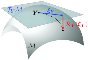
(a) Retraction

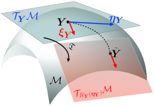
(b) Vector Transport

Figure 3: Riemannian retraction and vector transport operation.

A vector transport is defined by

$$\mathfrak{T}_{{\bm{\eta}}_{{\bm{Y}}}}({\bm{\xi}}_{{\bm{Y}}}):=D\mathcal{R}_{{\bm{Y}}}({\bm{\eta}}_{{\bm{Y}}})[{\bm{\xi}}_{{\bm{Y}}}]={\bm{\xi}}_{{\bm{Y}}}.$$ (54)

Among many good choices for $\beta_{k}$, we choose

$$\beta_{k}=\frac{g_{{\bm{Y}}_{k}}(\textrm{grad}f_{k},\textrm{grad}f_{k}-\mathfrak{T}_{\alpha_{k-1}{\bm{\eta}}_{k-1}}(\textrm{grad}f_{k-1}))}{g_{{\bm{Y}}_{k}}({\bm{\eta}}_{k-1},\textrm{grad}f_{k}-\mathfrak{T}_{\alpha_{k-1}{\bm{\eta}}_{k-1}}(\textrm{grad}f_{k-1}))},$$

which is a generalized version of Hestenes-Stiefel [37].

IV-C2 Riemannian Trust-Region Algorithm

When the search direction is chosen by solving the local second-order approximation of $f({\bm{Y}})$, it results in the Riemannian trust-region algorithm. We will find the updating vector ${\bm{\eta}}$ by solving the trust-region subproblem

$$\mathop{\textrm{minimize}}_{{\bm{\eta}}\in\mathcal{T}_{{\bm{Y}}_{k}}\mathcal{M}} m_{k}({\bm{\eta}})=f_{k}+g_{{\bm{Y}}_{k}}(\textrm{grad}f_{k},{\bm{\eta}})+\frac{1}{2}g_{{\bm{Y}}_{k}}(\textrm{Hess}f_{k}[{\bm{\eta}}],{\bm{\eta}})$$

subject to $$\|{\bm{\eta}}\|_{g}\leq\Delta_{k},$$ (55)

where $\Delta_{k}>0$ is the radius of the trust region and $\|{\bm{\eta}}\|_{g}=\sqrt{g_{{\bm{Y}}_{k}}({\bm{\eta}},{\bm{\eta}})}$. Note that the solution ${\bm{\eta}}$ becomes a candidate for updating. This is because we will select a proper $\Delta_{k}$, find the corresponding solution ${\bm{\eta}}_{k}$ of the trust-region subproblem and then update ${\bm{Y}}$ through

$${\bm{Y}}_{k+1}=\mathcal{R}_{{\bm{Y}}_{k}}({\bm{\eta}}_{k}).$$ (56)

The criterion for choosing $\Delta_{k}$ is based on evaluating

$$\rho_{k}=\frac{f_{k}-f(\mathcal{R}_{{\bm{Y}}_{k}}({\bm{\eta}}_{k}))}{m_{k}({\bm{0}})-m_{k}({\bm{\eta}}_{k})}.$$ (57)

When $\rho_{k}$ is very small, the radius of trust region $\Delta_{k}$ should be reduced because in this case the second-order approximation is too inaccurate. If $\rho_{k}$ is not very small, we shall accept $\Delta_{k}$ and ${\bm{\eta}}_{k}$ and reduce the trust region. If $\rho_{k}$ is close to 1, it m means that the second-order approximation models original objective function well. Hence, we can accept this step and expand the trust region. Likewise, if $\rho_{k}\ll 1$, we should also reject this step and increase $\Delta_{k}$. The trust-region subproblem can be solved by the truncated conjugate gradient [23, Sec 7.3.2] algorithm (see Algorithm 2).

Input: $\mathcal{B},\bm{b},{\bm{Y}}_{k},\Delta_{k}$. Parameters $\kappa,\theta>0$

Initialize: $\bm{\eta}^{0},{\bm{r}}_{0}=\textrm{grad}f_{k},{\bm{\delta}}_{0}=-{\bm{r}}_{0}$

while $\|{\bm{r}}_{j+1}\|_{g}>\|{\bm{r}}_{0}\|_{g}\min(\|{\bm{r}}_{0}\|_{g}^{\theta},\kappa)$ do

       if $g_{{\bm{Y}}_{k}}({\bm{\delta}}_{j},\textrm{Hess}f_{k}[{\bm{\delta}}_{j}])\leq 0$ then

            Compute $\tau=\arg\min m_{k}({\bm{\eta}}_{k})$ where ${\bm{\eta}}_{k}={\bm{\eta}}^{j}+\tau{\bm{\delta}}_{j}$ and $\|{\bm{\eta}}_{k}\|_{g}=\Delta_{k}$,

             return ${\bm{\eta}}$

       end if

      Set ${\bm{\eta}}^{j+1}={\bm{\eta}}^{j}+\alpha_{j}{\bm{\delta}}_{j}$ where $\alpha_{j}=\|{\bm{r}}_{j}\|_{g}^{2}/g_{{\bm{Y}}_{k}}({\bm{\delta}}_{j},\textrm{Hess}f_{k}[{\bm{\delta}}_{j}])$

       if $\|{\bm{\eta}}^{j+1}\|_{g}\geq{\Delta}_{k}$ then

            Set $\tau$ as the solution to $\|{\bm{\eta}}_{k}\|_{g}=\Delta_{k}$ where ${\bm{\eta}}_{k}={\bm{\eta}}^{j}+\tau{\bm{\delta}}_{j}$,

             return ${\bm{\eta}}_{k}$

       end if

      Set ${\bm{r}}_{j+1}={\bm{r}}_{j}+\alpha_{j}\textrm{Hess}f_{k}[{\bm{\delta}}_{j}]$,

       Set $\beta_{j+1}=\|{\bm{r}}_{j+1}\|_{g}^{2}/\|{\bm{r}}_{j}\|_{g}^{2}$,

       Set ${\bm{\delta}}_{j+1}=-{\bm{r}}_{j+1}+\beta_{j+1}{\bm{\delta}}_{j}$,

       $j\leftarrow j+1$

end while

Output: ${\bm{\eta}}={\bm{\eta}}_{k}$.

Algorithm 2 Truncated Conjugate Gradient Algorithm for (55)

Riemannian trust-region algorithm harnesses the second-order information of the problem. It admits a superlinear [23, Theorem 7.4.11] convergence rate locally and is robust to initial points. Since the objective function $f$ is exactly a quadratic function which satisfies the Lipschitz gradient condition and other assumptions in [24], we can always find an approximate second-order critical points by the Riemannian trust-region algorithm.

IV-D Computational Complexity Analysis

Riemannian conjugate gradient and Riemannian trust-region algorithm involve computing optimization ingredients at each iteration, for which we show their computational complexity.

• Evaluate the objective value $f({\bm{Y}})$. Since $\mathcal{B}(\cdot)$ involves a series of sparse matrix multiplication, we can compute it efficiently and the complexity of computing $f({\bm{Y}})$ is $\mathcal{O}(mnl)$.

• Compute the Riemannian gradient $\textrm{grad}f$ (44). This includes computing matrix multiplication in $\mathcal{O}(mnl)$ and horizontal projection $\Pi_{{\bm{Y}}}^{h}$ (39). Since complexity of solving the Lyapunov equation (40) is $\mathcal{O}(r^{3}+(m+n)r^{2})$, the overall complexity is $\mathcal{O}(mnl+(m+n)r^{2}+r^{3})$.

• Compute the Riemannian Hessian $\textrm{Hess}f$ (IV-B2). Its cost is also $\mathcal{O}(mnl+(m+n)r^{2}+r^{3})$.

• Computing the Riemannian metric $\overline{g}$ (37). This complexity is dominant by matrix multiplications, which is $\mathcal{O}((m+n)r^{2})$.

• Computational complexity of retraction $\overline{\mathcal{R}}$ (49) is $\mathcal{O}((m+n)r)$ and vector transport $\mathfrak{T}$ (54) is insignificant.

From the above results, we conclude that the computational complexity of Riemannian conjugate gradient algorithm for each iteration is $\mathcal{O}(mnl+(m+n)r^{2}+r^{3})$. And each iteration of truncated conjugate gradient algorithm also involves computation with complexity $\mathcal{O}(mnl+(m+n)r^{2}+r^{3})$.

V Simulations

This section presents numerical experiments to demonstrate the efficacy of the generalized low-rank optimization approach for topological cooperation via the newly presented Riemannian optimization algorithms. We will investigate the performance of different algorithms from the perspective of convergence rate and achievable DoF. We evaluate our model in different settings and demonstrate that the generalized low-rank approach can effectively enable transmitter cooperation based only on network topology information.

Our simulations compare the following matrix-factorization-based algorithms for solving the generalized low-rank optimization problem $\mathscr{P}$:

• “AltMin” [22]: Alternating minimization algorithm (20) (21) is adopted in [22] for topological transmitter cooperation problem by alternatively updating factors. For fixed $r$, (20) (21) are solved with gradient descent followed by backtracking line search.

• “RCG”: The Riemannian conjugate gradient method is developed in Sec IV-C1. We implement this algorithm with Manopt [38] software package.

• “RTR”: The Riemannian trust-region method is developed in Sec IV-C2 and also implemented with Manopt.

All algorithm are adopted with random initialization strategy for each rank $r$, and we find the minimal $r$ by increasing $r$ from 1 to $N$ until ${m}^{-0.5}\cdot\|\mathcal{A}({\bm{X}})-{\bm{b}}\|<10^{-3}$. In our numerical experiments, the network topology and shared messages at each transmitter are generated uniformly at random with probabilities

$$\textrm{Prob}((k,j)\in\mathcal{E})=\left\{\begin{aligned} &p,&&j\neq k\\ &1,&&j=k\end{aligned}\right.,$$ (58)

and

$$\textrm{Prob}(j\in\mathcal{S}_{k})=\left\{\begin{aligned} &q,&&j\neq k\\ &1,&&j=k\end{aligned}\right.,$$ (59)

respectively.

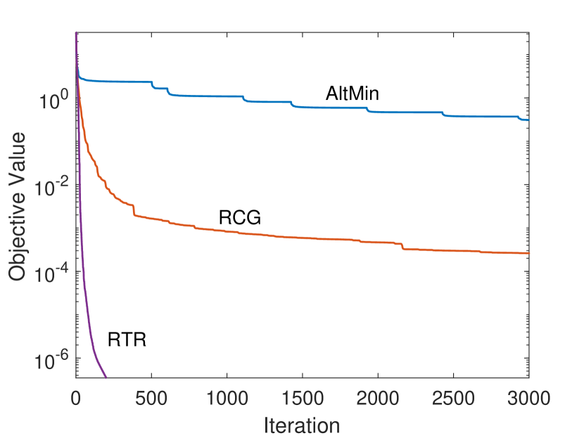
(a)

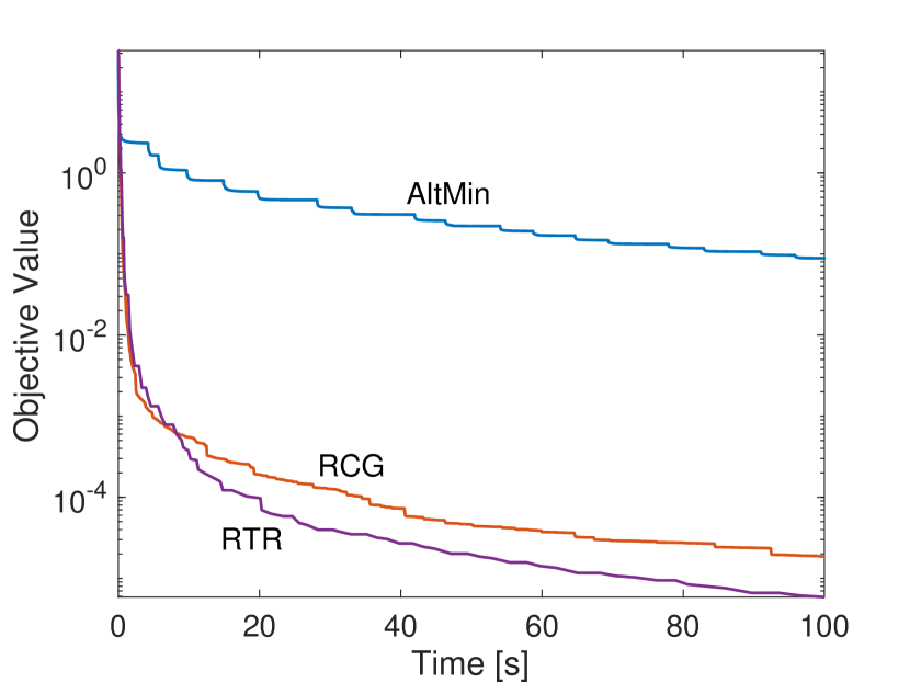
(b)

Figure 4: Convergence rate and computing time of all algorithms with full transmitter cooperation.

V-A Convergence Rate

Consider a partially connected $20$-user interference channel with full transmitter cooperation. The network topology is generated randomly and each link is connected with probability $p=0.3$. Each message is split into $3$ data streams. In this simulation, $K=20,d_{1}=\cdots=d_{K}=3$, $p=0.3$ and $r=12$. Fig. 4 shows the convergence behaviors of all 3 algorithms in terms of iterations and time. The results indicate that the proposed RTR algorithm exhibits a superlinear convergence rate, and the computing rate is comparable with first order RCG algorithm. In addition, the proposed RTR can yield a more accurate solution with the second-order stationary point when compared against first order algorithms that guarantee convergence only to first-order stationary points. The overall test results show that the proposed RTR and RCG algorithms are much more efficient than other contemporary algorithms in terms of convergence rates and solution performance.

To further show that the interferences are nulled, we choose the interference leakage as the metric and plot it in Fig. 5 for the same setting of Fig. 4. The interference leakage cost is given by

$$IL=\sum_{i\neq k}\sum_{j:(k,j)\in\mathcal{E},i\in\mathcal{S}_{j}}\!\!\!\!\!\!\!\|h_{kj}{\bm{U}}_{k}^{\sf{H}}{\bm{V}}_{ji}\Big{(}h_{kj}{\bm{U}}_{k}^{\sf{H}}{\bm{V}}_{ji}\Big{)}^{\sf{H}}\|_{F}^{2},$$ (60)

where the channel coefficients follow standard complex Gaussian distribution. Fig. 5 demonstrates that there is a rapid decline of interference leakage as the objective value decreases with the proposed Riemannian optimization algorithms.

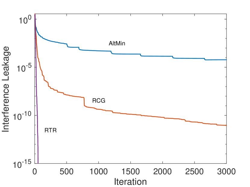
(a)

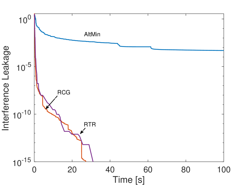
(b)

Figure 5: Convergence of interference leakage for all algorithms with full transmitter cooperation.

V-B DoF over Network Topologies

Consider a partially connected $20$-user interference channel without message splitting ($d_{k}=1$). The network topologies are generated randomly with different $p$. Fig. 6 demonstrates the DoF over $p$ with full transmitter cooperation. Each DoF result is averaged over 100 times. This result shows that, among the 3 solutions, the proposed RTR algorithm achieves the best performance with second-order stationary points. The Riemannian algorithms RTR and RCG significantly outperform the alternating minimization algorithm owing to their good convergence guarantee.

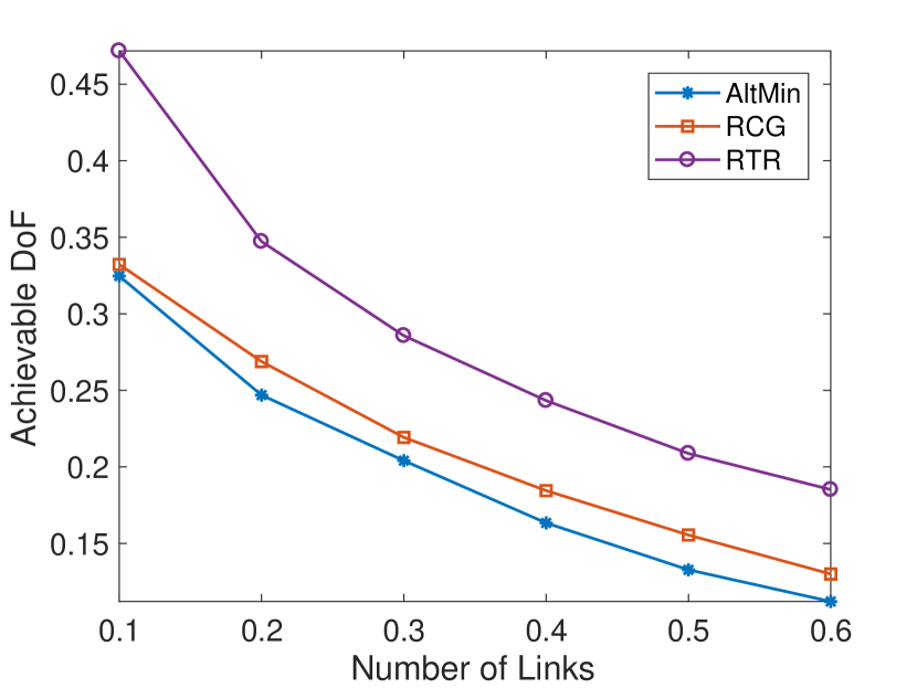
Figure 6: DoF over the number of connected links.

To further justify the effectiveness of the Riemannian optimization framework, we check the recovered DoF returned by the proposed RTR algorithm for all specific network topologies $\mathcal{E}$ and specific message sharing pattern $\{\mathcal{S}_{k}:k\in[K]\}$ provided in [14]. Specifically, transmitter cooperation improves the symmetric DoF from $1/3$ to $2/5$ for Example 1 in Fig. 1(a), from $2/5$ to $1/2$ for Example 4 in Fig. 3(a), and from $1/3$ to $2/5$ for Example 7 in Fig. 6(a), compared with the cases without cooperation. And the optimal symmetric DoF is $1/2$ for Example 6 in Fig. 5(a) with transmitter cooperation. All these optimal symmetric DoF results can be achieved by the proposed RTR algorithm numerically. However, theoretically identifying the network topologies and the message sharing patterns for which the Riemannian trust region algorithm can provide optimal symmetric DoFs is still a challenging open problem.

V-C Transmitter Cooperation Gains

We investigate the achievable DoFs in partially connected $20$-user interference channels. We randomly generate the network topologies with $p=0.2$ and simulate different algorithms under different transmitter cooperation level $q$ with single data stream. For each cooperation level, we take average over 500 channel realizations. Fig. 7a shows that the second-order algorithm RTR can achieve the highest DoF among all algorithms. Comparing the first-order algorithms, the proposed RCG outperforms AltMin. With the high convergence rate and second-order stationary points solutions of RTR, the gap between RTR algorithm and other algorithms grows with $q$, which indicates that the proposed RTR algorithm is capable of fully leveraging the benefits of transmitter cooperation.

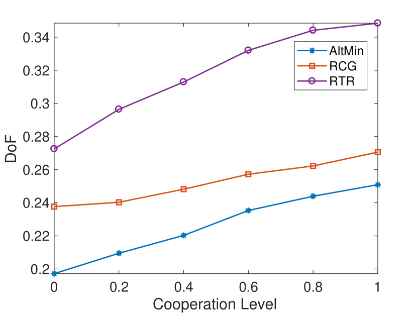
(a)

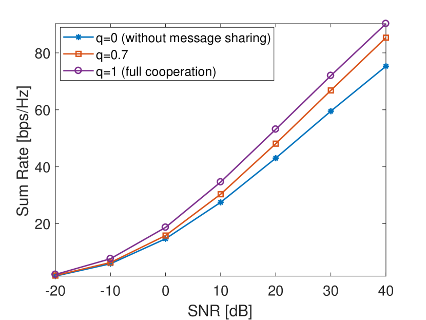
(b)

Figure 7: Benefits of transmitter cooperation: (a) DoF over different transmitters cooperation levels $q$. (b) Sum-rate over the transmit power.

To further illustrate the transmitter cooperation benefit, we evaluate the achievable sum-rate using the proposed RTR algorithm in Fig. 7a. In this single data stream test setting, ${\bm{U}}_{k},{\bm{V}}_{ji}$ degenerates to vectors ${\bm{u}}_{k},{\bm{v}}_{ji}$. Assume that each single data stream symbol $s_{i}$ has unit power, i.e., $\mathbb{E}(|s_{i}|^{2})=1$. Suppose the noise is i.i.d. Gaussian, i.e., ${\bm{\Sigma}}_{k}=\sigma^{2}{\bm{I}}_{r}$, with $\sigma^{2}$ at $-120$dB. The distance $d_{ij}$ between each connected transmitter-receiver pair $(j,i)$ is uniformly distributed in $[0.1,0.2]$ km. The fading channel model is given as

$$h_{ij}=10^{-L(d_{ij})/20}c_{ij},(i,j)\in\mathcal{E},$$ (61)

where the pass loss is given by $L(d_{ij})=128.1+37.6\log_{10}d_{ij}$ and the small scale fading coefficient is given by $c_{ij}\sim\mathcal{CN}(0,1)$. Then the sum rate per channel use is given by

$$C_{\text{sum}}=\frac{1}{r}\sum_{k=1}^{K}C_{k}=\frac{1}{r}\sum_{k=1}^{K}\log(1+\textrm{SINR}_{k}),$$ (62)

where

$$\textrm{SINR}_{k}=\frac{|\sum_{(k,j)\in\mathcal{E},k\in\mathcal{S}_{j}}h_{kj}{\bm{u}}_{k}^{\sf{H}}{\bm{v}}_{jk}|^{2}}{\sum_{i\neq k}|\sum_{(k,j)\in\mathcal{E},i\in\mathcal{S}_{j}}h_{kj}{\bm{u}}_{k}^{\sf{H}}{\bm{v}}_{ji}|^{2}+\|{\bm{u}}_{k}\|_{2}^{2}\sigma^{2}}.$$

Based on the singular value decomposition (SVD) ${\bm{X}}^{*}={\bm{U}}{\bm{\Sigma}}{\bm{V}}^{\sf{H}}$, the transmit beamformer is simply chosen as ${\bm{U}}{\bm{\Sigma}}^{\frac{1}{2}}$, and receive beamformer is given by ${\bm{V}}{\bm{\Sigma}}^{\frac{1}{2}}$ with power normalization. Fig. 7b shows the achievable sum-rate over different transmit power $P$. Each point is averaged across 100 channel realizations with random $\mathcal{E}$ ($p=0.2$). The result also demonstrates that the proposed RTR algorithm is capable of achieving high data rates by leveraging transmitter cooperation.

In summary, our numerical experiments demonstrate that the proposed Riemannian trust-region algorithm is capable of obtaining high-precision solutions with second-order stationary points, leading to high achievable DoFs and data rates. Furthermore, the computation time of RTR algorithm in medium scale problems is comparable with first order algorithms, which demonstrates that the proposed RTR algorithm is a powerful algorithm capable of harnessing the benefit of topological cooperation in problems involving medium network sizes.

VI Conclusions

This work investigates the opportunities of transmitter cooperation based only on topological information with message sharing. Our contributions include the derivation of a generalized topological interference alignment condition, followed by the development of a low-rank matrix optimization approach to maximize the achievable DoFs. To solve the resulting generalized low-rank optimization problem which is nonconvex in complex field, we developed Riemannian optimization algorithms by exploiting the complex non-compact Stiefel manifold for fixed-rank matrices in complex field. In particular, we adopted the semidefinite lifting technique and Burer-Monteiro factorization approach. Our experiments demonstrated that the proposed Riemannian algorithms considerably outperformed the alternating minimization algorithm. Additionally, the proposed Riemannian trust-region algorithm achieves high DoFs with high-precision second-order stationary point solutions, with computation complexity comparable with the first-order Riemannian conjugate gradient algorithm.

Appendix A Proof of Proposition 2

For simplicity, we only give the proof of the single data stream case, while it can be readily extended to general multiple data stream cases. In this case, ${\bm{X}}$ is given by

$${\bm{X}}=\begin{bmatrix}{\bm{u}}_{1}^{\sf{H}}{\bm{v}}_{11}&\cdots&{\bm{u}}_{1}^{\sf{H}}{\bm{v}}_{KK}\\ \vdots&\ddots&\vdots\\ {\bm{u}}_{K}^{\sf{H}}{\bm{v}}_{11}&\cdots&{\bm{u}}_{K}^{\sf{H}}{\bm{v}}_{KK}\end{bmatrix}\in\mathbb{C}^{K\times K^{2}}.$$ (63)

Let ${\bm{x}}_{i}$ denote the transpose of the $i$-th row of matrix ${\bm{X}}$. Problem (III-B1) can be rewritten as

$$\mathop{\textrm{minimize}}_{{{\bm{X}}}\in\mathbb{C}^{m\times n}} \|{{\bm{X}}}\|_{*}$$

subject to $$\bm{1}^{\sf{H}}{\bm{x}}_{k}^{\mathcal{D}_{k}}=1,~{}\forall k\in[K]$$ (64)

$${\bm{x}}_{k}^{\mathcal{G}_{k}}={\bm{0}},~{}\forall k\in[K],$$

in which ${\bm{x}}_{k}^{\mathcal{D}_{k}},{\bm{x}}_{k}^{\mathcal{G}_{k}}$ are vectors whose elements are sampled from ${\bm{x}}_{k}$, and $\mathcal{D}_{k},\mathcal{G}_{k}$ are the index sets of sampling. $\mathcal{D}_{k}$ and $\mathcal{G}_{k}$ are given by

$$\mathcal{D}_{k}=\{(j-1)*K+k:(k,j)\in\mathcal{E},k\in\mathcal{S}_{j}\}$$ (65)

and

$$\mathcal{G}_{k}=\{(j-1)*K+i:i\neq k,(k,j)\in\mathcal{E},i\in\mathcal{S}_{j}\},$$ (66)

respectively.

Lemma 1.

The optimal solution of (A), denoted by ${\bm{X}}^{\star}$, is given by

$${{\bm{x}}^{\star}}_{k}^{\mathcal{D}_{k}}=\frac{1}{|\mathcal{D}_{k}|}{{\bm{1}}},$$ (67)

where ${\bm{1}}$ denotes the vector of all ones. The remaining entries of ${\bm{X}}^{\star}$ are all zeros.

Proof.

Let $g({\bm{X}})=\|{\bm{X}}\|_{*}=\textrm{Tr}(\sqrt{{\bm{X}}{\bm{X}}^{\sf{H}}})$. To proof Lemma 1, it is equivalent to prove that $t=0$ is a minimum of the convex function

$$h(t)=\|{\bm{X}}^{\star}+t{\bm{X}}\|_{*},\mathcal{A}({\bm{X}}^{\star}+t{\bm{X}})={\bm{b}},t\in\mathbb{R}.$$ (68)

This can be deduced from the fact that any feasible point can be expressed as ${\bm{X}}^{\star}+t{\bm{X}}$, and if $t=0$ is a minimum of $h(t)$, then $g({\bm{X}}^{\star})\leq g({\bm{X}})$ always holds.

Based on the structure of $\mathcal{D}_{k}$ and $\mathcal{G}_{k}$, we have

$${\bm{X}}^{\star}{{\bm{X}}^{\star}}^{\sf{H}}=\begin{bmatrix}\frac{1}{|\mathcal{D}_{1}|}&0&\cdots&0\\ 0&\frac{1}{|\mathcal{D}_{2}|}&\cdots&0\\ \vdots&\vdots&\ddots&\vdots\\ 0&0&\cdots&\frac{1}{|\mathcal{D}_{K}|}\end{bmatrix}.$$ (69)

Then ${\bm{X}}^{\star}$ is a full rank matrix, and we can find $|t|\leq\epsilon$ such that ${\bm{X}}^{\star}+t{\bm{X}}$ is invertible. Therefore, the derivative of $h$ is given by

$$h^{\prime}(t)=\frac{1}{2}\big{\langle} \left(({\bm{X}}^{\star}+t{\bm{X}})({\bm{X}}^{\star}+t{\bm{X}})^{\sf{H}}\right)^{-\frac{1}{2}},$$

$${\bm{X}}{{\bm{X}}^{\star}}^{\sf{H}}+{\bm{X}}^{\star}{\bm{X}}^{\sf{H}}+2t{\bm{X}}{\bm{X}}^{\sf{H}}\big{\rangle}.$$ (70)

Then we have

$$h^{\prime}(0)=\frac{1}{2}\big{\langle}\left({\bm{X}}^{\star}{{\bm{X}}^{\star}}^{\sf{H}}\right)^{-\frac{1}{2}},{\bm{X}}{{\bm{X}}^{\star}}^{\sf{H}}+{\bm{X}}^{\star}{\bm{X}}^{\sf{H}}\big{\rangle}.$$ (71)

Since $\mathcal{A}({\bm{X}}^{\star}+t{\bm{X}})={\bm{b}}$, i.e.,

$$\bm{1}^{\sf{H}}({{\bm{x}}^{\star}}_{k}^{\mathcal{D}_{k}}+t{\bm{x}}_{k}^{\mathcal{D}_{k}})=1$$ (72)

then we have $\langle{{\bm{x}}^{\star}}_{k}^{\mathcal{D}_{k}},{\bm{x}}_{k}^{\mathcal{D}_{k}}\rangle=0$. Therefore,

$$\textrm{diag}({\bm{X}}{{\bm{X}}^{\star}}^{\sf{H}})=\textrm{diag}({\bm{X}}^{\star}{\bm{X}}^{\sf{H}})={\bm{0}}.$$ (73)

From (73) (69), we can deduce that $h^{\prime}(0)=0$, and thus $t=0$ is a minimum of $h(t)$. ∎

From Lemma 1 we know that the optimal solution ${\bm{X}}^{\star}$ of (III-B1) is full rank. So nuclear norm relaxation approach always fails.

Appendix B Proof of Proposition 4

The elements in the vertical space $\mathcal{V}_{{\bm{Y}}}$ must be tangential to the equivalent class $[{\bm{Y}}]=\{{\bm{Y}}{\bm{Q}}:{\bm{Q}}^{\sf{H}}{\bm{Q}}={\bm{I}}\}$. Let ${\bm{Y}}(t)={\bm{Y}}_{0}{\bm{Q}}(t)$ be a curve in $[{\bm{Y}}_{0}]$ through ${\bm{Y}}_{0}$ at $t=0$, i.e., ${\bm{Q}}(0)={\bm{I}}$. Then we have

$${\bm{Y}}(t){\bm{Y}}(t)^{\sf{H}}={\bm{Y}}_{0}{\bm{Q}}(t){\bm{Q}}(t)^{\sf{H}}{\bm{Y}}_{0}^{\sf{H}}={\bm{Y}}_{0}{\bm{Y}}_{0}^{\sf{H}}.$$ (74)

By differentiating (74) we get

$$\dot{{\bm{Y}}}(t){\bm{Y}}(t)^{\sf{H}}+{\bm{Y}}(t)\dot{{\bm{Y}}}(t)^{\sf{H}}={\bm{0}}.$$ (75)

So we deduce that $\dot{{\bm{Y}}}(0)$ belongs to

$$\{{\bm{Z}}\in\mathbb{C}^{N\times r}:{\bm{Z}}{\bm{Y}}_{0}^{\sf{H}}+{\bm{Y}}_{0}{\bm{Z}}^{\sf{H}}={\bm{0}}\},$$ (76)

of which $\mathcal{T}_{{\bm{Y}}}\mathcal{M}$ is a subset. On the other side, let $F:{\bm{Y}}\mapsto{\bm{Y}}{\bm{Y}}^{\sf{H}}$, then (76) is $\textrm{ker}(\textrm{D}F({\bm{Y_{0}}}))$ and $F^{-1}({\bm{Y}}_{0}{\bm{Y}}_{0}^{\sf{H}})=[{\bm{Y}}_{0}]$. Therefore, from [23, Sec 3.5.7] we know

$$\mathcal{T}_{{\bm{Y}}}\mathcal{M}=\{{\bm{Z}}\in\mathbb{C}^{N\times r}:{\bm{Z}}{\bm{Y}}_{0}^{\sf{H}}+{\bm{Y}}_{0}{\bm{Z}}^{\sf{H}}={\bm{0}}\}.$$ (77)

Without loss of generality, we can set

$$\dot{{\bm{Y}}}(t)={\bm{Y}}(t){\bm{\Omega}}(t),~{}~{}{\bm{\Omega}}(t)\in\mathbb{C}^{r\times r},$$ (78)

since ${\bm{Y}}(t)\in\mathbb{C}_{*}^{N\times r}$ is full rank. Then we can replace equation (78) in (75) and obtain

$${\bm{Y}}(t)({\bm{\Omega}}(t)+{\bm{\Omega}}(t)^{\sf{H}}){\bm{Y}}(t)^{\sf{H}}={\bm{0}}.$$ (79)

Therefore, the vertical space is given by

$$\mathcal{V}_{{\bm{Y}}}=\{{\bm{Y}}_{0}{\bm{\Omega}}:{\bm{\Omega}}^{\sf{H}}=-{\bm{\Omega}}\}.$$ (80)

Appendix C Proof of Proposition 5

The horizontal space is given by

$$\mathcal{H}_{{\bm{Y}}}=\{\overline{{\bm{\xi}}}\in\mathcal{T}_{{\bm{Y}}}\overline{\mathcal{M}}:\overline{g}_{{\bm{Y}}}(\overline{{\bm{\xi}}},\overline{{\bm{\zeta}}})=0,~{}\forall\overline{{\bm{\zeta}}}\in\mathcal{V}_{{\bm{Y}}}\},$$ (81)

that is

$$\overline{g}_{{\bm{Y}}}(\overline{{\bm{\xi}}},{\bm{Y}}{\bm{\Omega}})=0,\forall{\bm{\Omega}}^{\sf{H}}=-{\bm{\Omega}}.$$ (82)

Since

$$\overline{g}_{{\bm{Y}}}(\overline{{\bm{\xi}}},{\bm{Y}}{\bm{\Omega}}) ={\textrm{Tr}}(\overline{{\bm{\xi}}}^{\sf{H}}{\bm{Y}}{\bm{\Omega}}+{\bm{\Omega}}^{\sf{H}}{\bm{Y}}^{\sf{H}}\overline{{\bm{\xi}}})$$

$$={\textrm{Tr}}(\overline{{\bm{\xi}}}^{\sf{H}}{\bm{Y}}{\bm{\Omega}}-{\bm{\Omega}}{\bm{Y}}^{\sf{H}}\overline{{\bm{\xi}}})$$

$$={\textrm{Tr}}((\overline{{\bm{\xi}}}^{\sf{H}}{\bm{Y}}-{\bm{Y}}^{\sf{H}}\overline{{\bm{\xi}}}){\bm{\Omega}}),$$ (83)

we know the horizontal space consists of all the elements $\overline{{\bm{\xi}}}$ that satisfies ${\textrm{Tr}}((\overline{{\bm{\xi}}}^{\sf{H}}{\bm{Y}}-{\bm{Y}}^{\sf{H}}\overline{{\bm{\xi}}}){\bm{\Omega}})=0$ for all ${\bm{\Omega}}^{\sf{H}}=-{\bm{\Omega}}$. Therefore, the horizontal space is

$$\mathcal{H}_{{\bm{Y}}}=\{{\bm{\xi}}\in\mathbb{C}^{N\times r}:{\bm{\xi}}^{\sf{H}}{\bm{Y}}={\bm{Y}}^{\sf{H}}{\bm{\xi}}\}.$$ (84)

Suppose for a vecor ${\bm{\xi}}\in\mathcal{T}_{{\bm{Y}}}\mathcal{M}$ its projection onto the vertical space is given by ${\bm{\xi}}^{v}={\bm{Y}}{\bm{\Omega}}_{{\bm{\xi}}}$, then the horizontal projection is given by ${\bm{\xi}}^{h}={\bm{\xi}}-{\bm{Y}}{\bm{\Omega}}_{{\bm{\xi}}}$, and

$${{\bm{\xi}}^{h}}^{\sf{H}}{\bm{Y}}={\bm{Y}}^{\sf{H}}{{\bm{\xi}}^{h}}.$$ (85)

So we can find the ${\bm{\Omega}}_{{\bm{\xi}}}$ from

$$({\bm{\xi}}-{\bm{Y}}{\bm{\Omega}}_{{\bm{\xi}}})^{\sf{H}}{\bm{Y}}={\bm{Y}}^{\sf{H}}({\bm{\xi}}-{\bm{Y}}{\bm{\Omega}}_{{\bm{\xi}}})$$

$$\Rightarrow~{} {\bm{Y}}^{\sf{H}}{\bm{Y}}{\bm{\Omega}}_{{\bm{\xi}}}+{\bm{\Omega}}_{{\bm{\xi}}}{\bm{Y}}^{\sf{H}}{\bm{Y}}={\bm{Y}}^{\sf{H}}{\bm{\xi}}-{\bm{\xi}}^{\sf{H}}{\bm{Y}}.$$ (86)

Then we conclude that the horizontal projection of ${\bm{\xi}}$ is given by

$$\Pi_{{\bm{Y}}}^{h}{\bm{\xi}}={\bm{\xi}}-{\bm{Y}}{\bm{\Omega}},$$ (87)

where ${\bm{\Omega}}$ is the solution to the Lyapunov equation

$${\bm{Y}}^{\sf{H}}{\bm{Y}}{\bm{\Omega}}+{\bm{\Omega}}{\bm{Y}}^{\sf{H}}{\bm{Y}}={\bm{Y}}^{\sf{H}}{\bm{\xi}}-{\bm{\xi}}^{\sf{H}}{\bm{Y}}.$$ (88)

Appendix D Computing the Riemannian Gradient and Hessian

We first rewrite the objective function of (28) as

$$f({\bm{Y}})=\frac{1}{2}\sum_{i=1}^{l}|\langle{\bm{B}}_{i},{\bm{Y}}{\bm{Y}}^{\sf{H}}\rangle-b_{i}|^{2}.$$ (89)

The complex gradient of $f({\bm{Y}})$ is given by

$$f^{\prime}({\bm{Y}}) =\sum_{i=1}^{l}(\langle{\bm{B}}_{i},{\bm{Y}}{\bm{Y}}^{\sf{H}}\rangle-b_{i}){\bm{B}}_{i}{\bm{Y}}+(\langle{\bm{B}}_{i}^{\sf{H}},{\bm{Y}}{\bm{Y}}^{\sf{H}}\rangle-b_{i}^{*}){\bm{B}}_{i}^{\sf{H}}{\bm{Y}}$$

$$=\sum_{i=1}^{l}(C_{i}{\bm{B}}_{i}+C_{i}^{*}{\bm{B}}_{i}^{\sf{H}}){\bm{Y}},$$ (90)

in which $C_{i}=\langle{\bm{B}}_{i},{\bm{Y}}{\bm{Y}}^{\sf{H}}\rangle-b_{i}$. The Riemannian gradient $\overline{\textrm{grad}}f({\bm{Y}})$ is derived from (43), and we find that

$$\textrm{D}f({\bm{Y}})[{\bm{\xi}}] =\frac{1}{2}\sum_{i=1}^{l}\langle{\bm{B}}_{i},{\bm{\xi}}{\bm{Y}}^{\sf{H}}+{\bm{Y}}{\bm{\xi}}^{\sf{H}}\rangle^{*}(\langle{\bm{B}}_{i},{\bm{Y}}{\bm{Y}}^{\sf{H}}\rangle-b_{i})$$

$$\qquad+(\langle{\bm{B}}_{i},{\bm{Y}}{\bm{Y}}^{\sf{H}}\rangle-b_{i})^{*}\langle{\bm{B}}_{i},{\bm{\xi}}{\bm{Y}}^{\sf{H}}+{\bm{Y}}{\bm{\xi}}^{\sf{H}}\rangle$$

$$=\overline{g}_{{\bm{Y}}}((C_{i}{\bm{B}}_{i}+C_{i}^{*}{\bm{B}}_{i}^{\sf{H}}){\bm{Y}},{\bm{\xi}}).$$ (91)

Therefore, $\overline{\textrm{grad}}f({\bm{Y}})=f^{\prime}({\bm{Y}})$. Then we observe that $\overline{\textrm{grad}}f({\bm{Y}})^{\sf{H}}{\bm{Y}}={\bm{Y}}^{\sf{H}}\overline{\textrm{grad}}f({\bm{Y}})$, i.e., $\overline{\textrm{grad}}f({\bm{Y}})$ is already in the horizontal space $\mathcal{V}_{{\bm{Y}}}$. So the horizontal representation of Riemannian gradient is given by

$$\textrm{grad}f({\bm{Y}})=\sum_{i=1}^{l}(C_{i}{\bm{B}}_{i}+C_{i}^{*}{\bm{B}}_{i}^{\sf{H}}){\bm{Y}}.$$ (92)

To derive the Riemannian Hessian (46), we compute

$$\textrm{D}\overline{\textrm{grad}}f({\bm{Y}})[{\bm{\eta}}_{{\bm{Y}}}]=\sum_{i=1}^{l}( {C_{{\bm{\eta}}}}_{i}{\bm{B}}_{i}{\bm{Y}}+C_{i}{\bm{B}}_{i}{\bm{\eta}}_{Y}$$

$$+{C_{{\bm{\eta}}}}_{i}^{*}{\bm{B}}_{i}^{\sf{H}}{\bm{Y}}+C_{i}^{*}{\bm{B}}_{i}^{\sf{H}}{\bm{\eta}}_{\bm{Y}}),$$ (93)

where ${C_{{\bm{\eta}}}}_{i}=\langle{\bm{B}}_{i},{\bm{Y}}{\bm{\eta}}_{\bm{Y}}^{\sf{H}}+{\bm{\eta}}_{\bm{Y}}{\bm{Y}}^{\sf{H}}\rangle$. We conclude that

$$\textrm{Hess}f({\bm{Y}})[{\bm{\eta}}_{{\bm{Y}}}]=\Pi_{{\bm{Y}}}^{h}\biggl{(} \sum_{i=1}^{l}({C_{{\bm{\eta}}}}_{i}{\bm{B}}_{i}{\bm{Y}}+C_{i}{\bm{B}}_{i}{\bm{\eta}}_{Y}$$

$$+{C_{{\bm{\eta}}}}_{i}^{*}{\bm{B}}_{i}^{\sf{H}}{\bm{Y}}+C_{i}^{*}{\bm{B}}_{i}^{\sf{H}}{\bm{\eta}}_{\bm{Y}})\biggr{)}.$$ (94)

References

- [1] M. Simsek, A. Aijaz, M. Dohler, J. Sachs, and G. Fettweis, “5G-enabled tactile internet,” IEEE J. Sel. Areas Commun., vol. 34, no. 3, pp. 460–473, Mar. 2016.
- [2] Y. Shi, J. Zhang, B. O’Donoghue, and K. B. Letaief, “Large-scale convex optimization for dense wireless cooperative networks,” IEEE Trans. Signal Process., vol. 63, no. 18, pp. 4729–4743, Sept. 2015.
- [3] V. R. Cadambe and S. A. Jafar, “Interference alignment and degrees of freedom of the -user interference channel,” IEEE Trans. Inf. Theory, vol. 54, no. 8, pp. 3425–3441, Aug. 2008.
- [4] D. Gesbert, S. Hanly, H. Huang, S. S. Shitz, O. Simeone, and W. Yu, “Multi-cell MIMO cooperative networks: A new look at interference,” IEEE J. Sel. Areas Commun., vol. 28, no. 9, pp. 1380–1408, Dec. 2010.
- [5] Y. Shi, J. Zhang, and K. B. Letaief, “Group sparse beamforming for green Cloud-RAN,” IEEE Trans. Wireless Commun., vol. 13, no. 5, pp. 2809–2823, May 2014.
- [6] K. Yang, Y. Shi, and Z. Ding, “Generalized matrix completion for low complexity transceiver processing in cache-aided Fog-RAN via the Burer-Monteiro approach,” Proc. IEEE Global Conf. Signal Inf. Process. (GlobalSIP), 2017.
- [7] M. A. Maddah-Ali and U. Niesen, “Fundamental limits of caching,” IEEE Trans. Inf. Theory, vol. 60, no. 5, pp. 2856–2867, May 2014.
- [8] M. A. Maddah-Ali and D. Tse, “Completely stale transmitter channel state information is still very useful,” IEEE Trans. Inf. Theory, vol. 58, no. 7, pp. 4418–4431, Jul. 2012.
- [9] Y. Shi, J. Zhang, and K. B. Letaief, “Optimal stochastic coordinated beamforming for wireless cooperative networks with CSI uncertainty,” IEEE Trans. Signal Process., vol. 63, no. 4, pp. 960–973, Feb. 2015.
- [10] M. Razaviyayn, M. Sanjabi, and Z.-Q. Luo, “A stochastic successive minimization method for nonsmooth nonconvex optimization with applications to transceiver design in wireless communication networks,” Math. Program., vol. 157, no. 2, pp. 515–545, Jun. 2016.
- [11] A. G. Davoodi and S. A. Jafar, “Generalized degrees of freedom of the symmetric -user interference channel under finite precision CSIT,” IEEE Trans. Inf. Theory, vol. 63, no. 10, pp. 6561–6572, Oct. 2017.
- [12] W. U. Bajwa, J. Haupt, A. M. Sayeed, and R. Nowak, “Compressed channel sensing: A new approach to estimating sparse multipath channels,” Proc. IEEE, vol. 98, no. 6, pp. 1058–1076, Jun. 2010.
- [13] S. A. Jafar, “Topological interference management through index coding,” IEEE Trans. Inf. Theory, vol. 60, no. 1, pp. 529–568, Jan. 2014.
- [14] X. Yi and D. Gesbert, “Topological interference management with transmitter cooperation,” IEEE Trans. Inf. Theory, vol. 61, no. 11, pp. 6107–6130, Nov. 2015.
- [15] Y. Shi, J. Zhang, and K. B. Letaief, “Low-rank matrix completion for topological interference management by Riemannian pursuit,” IEEE Trans. Wireless Commun., vol. 15, no. 7, pp. 4703–4717, Jul. 2016.
- [16] M. A. Davenport and J. Romberg, “An overview of low-rank matrix recovery from incomplete observations,” IEEE J. Sel. Topics Signal Process., vol. 10, no. 4, pp. 608–622, Jun. 2016.
- [17] G. Sridharan and W. Yu, “Linear beamformer design for interference alignment via rank minimization,” IEEE Trans. Signal Process., vol. 63, no. 22, pp. 5910–5923, Nov. 2015.
- [18] D. S. Papailiopoulos and A. G. Dimakis, “Interference alignment as a rank constrained rank minimization,” IEEE Trans. Signal Process., vol. 60, no. 8, pp. 4278–4288, Aug. 2012.
- [19] E. J. Candès and B. Recht, “Exact matrix completion via convex optimization,” Found. Comput. Math., vol. 9, no. 6, p. 717, Apr. 2009.
- [20] P. Jain, P. Netrapalli, and S. Sanghavi, “Low-rank matrix completion using alternating minimization,” in Proc. ACM Symp. Theory Comput. (STOC), 2013, pp. 665–674.
- [21] R. Ge, J. D. Lee, and T. Ma, “Matrix completion has no spurious local minimum,” in Proc. Adv. Neural Inf. Process. Syst. (NIPS), 2016, pp. 2973–2981.
- [22] X. Yi and G. Caire, “Topological coded caching,” in Proc. IEEE Int. Symp. Inf. Theory (ISIT), Jul. 2016, pp. 2039–2043.
- [23] P.-A. Absil, R. Mahony, and R. Sepulchre, Optimization algorithms on matrix manifolds. Princeton Univ. Press, 2009.
- [24] N. Boumal, P.-A. Absil, and C. Cartis, “Global rates of convergence for nonconvex optimization on manifolds,” IMA J. Numerical Anal., to appear.
- [25] R. Ge, C. Jin, and Y. Zheng, “No spurious local minima in nonconvex low rank problems: A unified geometric analysis,” Proc. Int. Conf. Mach. Learn. (ICML), to appear.
- [26] S. Burer and R. D. Monteiro, “A nonlinear programming algorithm for solving semidefinite programs via low-rank factorization,” Math. Program., vol. 95, no. 2, pp. 329–357, Feb. 2003.
- [27] G. Bresler, D. Cartwright, and D. Tse, “Feasibility of interference alignment for the MIMO interference channel,” IEEE Trans. Inf. Theory, vol. 60, no. 9, pp. 5573–5586, Sept. 2014.
- [28] M. Razaviyayn, G. Lyubeznik, and Z. Q. Luo, “On the degrees of freedom achievable through interference alignment in a MIMO interference channel,” IEEE Trans. Signal Process., vol. 60, no. 2, pp. 812–821, Feb. 2012.
- [29] H. Babak, “Topological interference alignment in wireless networks,” in Smart Antennas Workshop, Aug. 2014.
- [30] Y. Zhang and Z. Lu, “Penalty decomposition methods for rank minimization,” in Proc. Adv. Neural Inf. Process. Syst. (NIPS), 2011, pp. 46–54.
- [31] S. Boyd and L. Vandenberghe, Convex optimization. Cambridge Univ. Press, 2004.
- [32] B. O’Donoghue, E. Chu, N. Parikh, and S. Boyd, “Conic optimization via operator splitting and homogeneous self-dual embedding,” J. Optim. Theory Appl., vol. 169, no. 3, pp. 1042–1068, Jun 2016.
- [33] Y. Shi, B. Mishra, and W. Chen, “Topological interference management with user admission control via riemannian optimization,” IEEE Trans. Wireless Commun., vol. 16, no. 11, pp. 7362–7375, Nov. 2017.
- [34] M. Journée, F. Bach, P. Absil, and R. Sepulchre, “Low-rank optimization on the cone of positive semidefinite matrices,” SIAM J. Optim., vol. 20, no. 5, pp. 2327–2351, 2010.
- [35] S. Yatawatta, “Radio interferometric calibration using a Riemannian manifold,” in Proc. IEEE Int. Conf. Acoustics Speech Signal Process. (ICASSP), May 2013, pp. 3866–3870.
- [36] W. Barth, K. Hulek, C. Peters, and A. Van de Ven, Compact complex surfaces. Springer, 2015, vol. 4.
- [37] M. R. Hestenes and E. Stiefel, “Methods of conjugate gradients for solving linear systems,” J. Res. National Bureau Standards, vol. 49, no. 1, pp. 409–435, 1952.
- [38] N. Boumal, B. Mishra, P.-A. Absil, and R. Sepulchre, “Manopt, a matlab toolbox for optimization on manifolds,” J. Mach. Learn. Res., vol. 15, no. 1, pp. 1455–1459, 2014.